Frequentist and Bayesian measures of confidence via multiscale bootstrap for testing three regions

Abstract.

A new computation method of frequentist $p$-values and Bayesian posterior probabilities based on the bootstrap probability is discussed for the multivariate normal model with unknown expectation parameter vector. The null hypothesis is represented as an arbitrary-shaped region. We introduce new parametric models for the scaling-law of bootstrap probability so that the multiscale bootstrap method, which was designed for one-sided test, can also computes confidence measures of two-sided test, extending applicability to a wider class of hypotheses. Parameter estimation is improved by the two-step multiscale bootstrap and also by including higher-order terms. Model selection is important not only as a motivating application of our method, but also as an essential ingredient in the method. A compromise between frequentist and Bayesian is attempted by showing that the Bayesian posterior probability with an noninformative prior is interpreted as a frequentist $p$-value of “zero-sided” test.

1. Introduction

Let $Y=(Y_{1},\ldots,Y_{m+1})$ be a random vector of dimension $m+1$ for some integer $m\geq 1$, and $y=(y_{1},\ldots,y_{m+1})\in\mathbb{R}^{m+1}$ be its observed value. Our argument is based on the multivariate normal model with unknown mean vector $\mu=(\mu_{1},\ldots,\mu_{m+1})\in\mathbb{R}^{m+1}$ and covariance identity $I_{m+1}$,

(1) $$Y\sim N_{m+1}(\mu,I_{m+1}),$$

where the probability with respect to (1) will be denoted as $P(\cdot|\mu)$. Let ${H}_{0}\subset\mathbb{R}^{m+1}$ be an arbitrary-shaped region. The subject of this paper is to compute measures of confidence for testing the null hypothesis $\mu\in{H}_{0}$. Observing $y$, we compute a frequentist $p$-value, denoted $p({H}_{0}|y)$, and also a Bayesian posterior probability $\pi({H}_{0}|y)$ with a noninformative prior density $\pi(\mu)$ of $\mu$.

This is the problem of regions discussed in literature; Efron et al (1996), Efron and Tibshirani (1998), and Shimodaira (2002, 2004, 2008). The confidence measures were calculated by the bootstrap methods for complicated application problems such as the variable selection of regression analysis and phylogenetic tree selection of molecular evolution. These model selection problems are motivating applications for the issues discussed in this paper, and the normal model of (1) is a simplification of reality. Let ${\cal X}=\{x_{1},\ldots,x_{n}\}$ be a sample of size $n$ in application problems. We assume there exists a transformation, depending on $n$, from ${\cal X}$ to $y$ so that $Y$ is approximately normalized. We assume only the existence of such a transformation, and do not have to consider its details. Since we work only on the transformed variable $Y$ in this paper for developing the theory, readers may refer to the literature above for the examples of applications. Before the problem formulation is given in Section 2, our methodology is illustrated in simple examples below in this section.

The simplest example of ${H}_{0}$ would be the half space of $\mathbb{R}^{m+1}$,

(2) $${H}_{0}^{\prime}:\mu_{m+1}\leq 0,$$

where the notation ${H}_{0}^{\prime}$, instead of ${H}_{0}$, is used to distinguish this case from another example given in (3). Only $\mu_{m+1}$ is involved in this ${H}_{0}^{\prime}$, and one-dimensional normal model $Y_{m+1}\sim N(\mu_{m+1},1)$ is considered. Taking $\mu_{m+1}>0$ as an alternative hypothesis and denoting the cumulative distribution function of the standard normal as $\Phi(\cdot)$ with density $\phi(\cdot)$, the unbiased frequentist $p$-value is given as $p({H}_{0}^{\prime}|y)=\Phi(-y_{m+1})$.

A slightly complex example of ${H}_{0}$ is

(3) $${H}_{0}:-d\leq\mu_{m+1}\leq 0$$

for $d>0$. The rejection regions are $y_{m+1}>c$ and $y_{m+1}<-d-c$ with a critical constant $c$, which is obtained as a solution of the equation

(4) $$\Phi(-c)+\Phi(-d-c)=\alpha$$

for a specified significance level $0<\alpha<1$. The left hand side of (4) is the rejection probability $P(Y_{m+1}>c\vee Y_{m+1}<-d-c|\mu)$ when $\mu$ is on the boundary of ${H}_{0}$, i.e., $\mu_{m+1}=0$ or $\mu_{m+1}=-d$. The frequentist $p$-value is defined as the infimum of $\alpha$ such that ${H}_{0}$ can be rejected. This becomes $p({H}_{0}|y)=\Phi(-y_{m+1})+\Phi(-d-y_{m+1})$ for $y_{m+1}\geq-d/2$ and $p({H}_{0}|y)=\Phi(y_{m+1})+\Phi(d+y_{m+1})$ for $y_{m+1}\leq-d/2$. Considering the case, say,

(5) $$d=1,\quad y_{m+1}=-0.1,$$

we obtain $p({H}_{0}^{\prime}|y)=0.540$ and $p({H}_{0}|y)=0.724$.

These two simple cases of ${H}_{0}$ and ${H}_{0}^{\prime}$ exhibit what Efron and Tibshirani (1998) called paradox of frequentist $p$-values. Our simple examples of (2) and (3) suffice for this purpose, although they had actually used the spherical shell example explained later in Section 4. Efron and Tibshirani (1998) indicated that a confidence measure should be monotonically increasing in the order of set inclusion of the hypothesis. Noting ${H}_{0}\subset{H}_{0}^{\prime}$, therefore, it should be $p({H}_{0}|y)\leq p({H}_{0}^{\prime}|y)$, but it is not. This kind of “paradox” cannot occur with Bayesian methods, and $\pi({H}_{0}|y)\leq\pi({H}_{0}^{\prime}|y)$ holds always. Considering the flat prior $\pi(\mu)=$ const, say, the posterior distribution of $\mu$ given $y$ becomes

(6) $$\mu|y\sim N_{m+1}(y,I_{m+1}),$$

and the posterior probabilities for the case (5) are $\pi({H}_{0}^{\prime}|y)=\Phi(-y_{m+1})=0.540$ and $\pi({H}_{0}|y)=\Phi(-y_{m+1})-\Phi(-d-y_{m+1})=0.356$. The “paradox” of frequentist $p$-values may be nothing surprise for a frequentist statistician, but a natural consequence of the fact that $p({H}_{0}^{\prime}|y)$ is for a one-sided test and $p({H}_{0}|y)$ is for a two-sided test; The power of testing is higher, i.e., $p$-values are smaller, for an appropriately formulated one-sided test than a two-sided test. In this paper, we do not intend to argue the philosophical question of whether to be frequentist or to be Bayesian, but discuss only computation of these two confidence measures.

Computation of the confidence measures is made by the bootstrap resampling of Efron (1979). Let ${\cal X}^{*}=\{x_{1}^{*},\ldots,x_{n^{\prime}}^{*}\}$ be a bootstrap sample of size $n^{\prime}$ obtained by resampling with replacement from ${\cal X}$. The idea of bootstrap probability, which is introduced first by Felsenstein (1985) to phylogenetic inference, is to generate ${\cal X}^{*}$ many times, say $B$, and count the frequency $C$ that a hypothesis of interest is supported by the bootstrap samples. The bootstrap probability is computed as $C/B$. Recalling the transformation to get $y$ from ${\cal X}$, we get $Y^{*}$ by applying the same transformation to ${\cal X}^{*}$. For typical problems, the variance of $Y^{*}$ is approximately proportional to the factor

$$\sigma^{2}=\frac{n}{n^{\prime}}$$

as mentioned in Shimodaira (2008). Although we generate ${\cal X}^{*}$ in practice, we only work on $Y^{*}$ in this paper. More specifically, we formally consider the parametric bootstrap

(7) $$Y^{*}|y\sim N_{m+1}(y,\sigma^{2}I_{m+1}),$$

which is analogous to (1) but the scale $\sigma$ is introduced for multiscale bootstrap. The bootstrap probability is defined as

(8) $$\alpha_{\sigma^{2}}({H}_{0}|y)=P_{\sigma^{2}}(Y^{*}\in{H}_{0}|y),$$

where $P_{\sigma^{2}}(\cdot|y)$ denotes the probability with respect to (7). For computing a crude confidence measure, we set $\sigma=1$, or $n^{\prime}=n$ in terms of ${\cal X}^{*}$, so that the distribution (7) for $Y^{*}$ is equivalent to the posterior (6) for $\mu$. This gives an interpretation of the bootstrap probability that $\alpha_{1}({H}_{0}|y)=\pi({H}_{0}|y)$ for any ${H}_{0}$ under the flat prior. In the multiscale bootstrap of Shimodaira (2002, 2004, 2008), however, we may intentionally alter the scale from $\sigma=1$, or to change $n^{\prime}$ from $n$ in terms of ${\cal X}^{*}$ for computing $p({H}_{0}|y)$. Let $\sigma_{1},\ldots,\sigma_{M}$ be $M$ different values of scale, which we specify in advance. In our numerical examples, $M=13$ scales are equally spaced in log-scale between $\sigma_{1}=1/3$ and $\sigma_{13}=3$. For each $i=1,\ldots,M$, we generate ${\cal X}^{*}$ with scale $\sigma_{i}$ for $B_{i}$ times, and observe the frequency $C_{i}$. The observed bootstrap probability is $\hat{\alpha}_{\sigma^{2}_{i}}=C_{i}/B_{i}$.

How can we use the observed $\hat{\alpha}_{\sigma^{2}_{1}},\ldots,\hat{\alpha}_{\sigma^{2}_{M}}$ for computing $p({H}_{0}|y)$? Let us assume that ${H}_{0}$ can be expressed as (3) but we are unable to observe the values of $y_{m+1}$ and $d$. Nevertheless, by fitting the model $\alpha_{\sigma^{2}}({H}_{0}|y)=\Phi(-y_{m+1}/\sigma)-\Phi(-(d+y_{m+1})/\sigma)$ to the observed $\hat{\alpha}_{\sigma^{2}_{1}},\ldots,\hat{\alpha}_{\sigma^{2}_{M}}$, we may compute an estimate $\hat{\varphi}$ of the parameter vector $\varphi=(y_{m+1},d)$ with constraints $d>0$ and $y_{m+1}>-d/2$. The confidence measures are then computed as $p({H}_{0}|y)=\Phi(-\hat{y}_{m+1})+\Phi(-\hat{d}-\hat{y}_{m+1})$ and $\pi({H}_{0}|y)=\Phi(-\hat{y}_{m+1})-\Phi(-\hat{d}-\hat{y}_{m+1})$. In case we are not sure which of (2) and (3) is the reality, we may also fit $\alpha_{\sigma^{2}}({H}_{0}^{\prime}|y)=\Phi(-y_{m+1}/\sigma)$ to the observed $\hat{\alpha}_{\sigma^{2}_{i}}$’s and compare the AIC values (Akaike, 1974) for model selection. In practice, we prepare collection of such models describing the scaling-law of bootstrap probability, and choose the model which minimizes the AIC value.

2. Formulation of the problem

The examples in Section 1 were very simple because the boundary surfaces of the regions are flat. In the following sections, we work on generalizations of (2) and (3) by allowing curved boundary surfaces. For convenience, we denote $y=(u,v)$ with $u=(y_{1},\ldots,y_{m})$ and $v=y_{m+1}$. Similarly, we denote $\mu=(\theta,\mu_{m+1})$ with $\theta=(\mu_{1},\ldots,\mu_{m})\in\mathbb{R}^{m}$. As shown in Fig. 1, we consider the region of the form ${H}_{0}=\{(\theta,\mu_{m+1})\mid-d-h_{2}(\theta)\leq\mu_{m+1}\leq-h_{1}(\theta),\,\theta\in\mathbb{R}^{m}\}$, where $h_{1}(\theta)$ and $h_{2}(\theta)$ are arbitrary functions of $\theta$. This region will reduce to (3) if $h_{1}(\theta)=h_{2}(\theta)=0$ for all $\theta$. The region may be abbreviated as

(9) $${H}_{0}:-d-h_{2}(\theta)\leq\mu_{m+1}\leq-h_{1}(\theta).$$

Two other regions ${H}_{1}:\mu_{m+1}\geq-h_{1}(\theta)$ and ${H}_{2}:\mu_{m+1}\leq-d-h_{2}(\theta)$ as well as two boundary surfaces $\partial{H}_{1}:\mu_{m+1}=-h_{1}(\theta)$ and $\partial{H}_{2}:\mu_{m+1}=-d-h_{2}(\theta)$ are also shown in Fig. 1. We define ${H}_{0}^{\prime}={H}_{0}\cup{H}_{2}$, or equivalently as

(10) $${H}_{0}^{\prime}:\mu_{m+1}\leq-h_{1}(\theta).$$

The boundary surfaces of the hypotheses are $\partial{H}_{0}=\partial{H}_{1}\cup\partial{H}_{2}$ for the region ${H}_{0}$, and $\partial{H}^{\prime}_{0}=\partial{H}_{1}$ for the region ${H}^{\prime}_{0}$.

We do not have to specify the functional forms of $h_{1}$ and $h_{2}$ for our theory, but assume that the magnitude of $h_{1}$ and $h_{2}$ is very small. Technically speaking, $h_{1}$ and $h_{2}$ are nearly flat in the sense of Shimodaira (2008). Introducing an artificial parameter $\lambda$, a function $h$ is called nearly flat when $\sup_{\theta\in\mathbb{R}^{m}}|h(\theta)|=O(\lambda)$ and $L^{1}$-norms of $h$ and its Fourier transform are bounded. We develop asymptotic theory as $\lambda\to 0$, which is analogous to $n\to\infty$ with the relation $\lambda=1/\!\sqrt{n}$.

The whole parameter space is partitioned into two regions as ${H}_{0}^{\prime}\cup{H}_{1}=\mathbb{R}^{m+1}$ or three regions as ${H}_{0}\cup{H}_{1}\cup{H}_{2}=\mathbb{R}^{m+1}$. These partitions are treated as disjoint in this paper by ignoring measure-zero sets such as ${H}_{0}^{\prime}\cap{H}_{1}=\partial{H}_{1}$. Bootstrap methods for computing frequentist confidence measures are well developed in the literature as reviewed in Section 3. The main contribution of our paper is then given in Section 4 for the case of three regions. In Section 5, this new computation method is used also for Bayesian measures of Efron and Tibshirani (1998). Note that the flat prior $\pi(\mu)=$ const in the previous section was in fact carefully chosen so that $\pi({H}_{0}^{\prime}|y)=p({H}_{0}^{\prime}|y)$ for (2). This same $\pi(\mu)$ led to $\pi({H}_{0}|y)\neq p({H}_{0}|y)$ for (3). Our definition of ${H}_{0}$ given in (9) is a simplest formulation, yet with a reasonable generality for applications, to observe such an interesting difference between the two confidence measures.

Multiscale bootstrap computation of the confidence measures for the three regions case is described in Section 6. Simulation study and some discussions are given in Section 7 and 8, respectively. Mathematical proofs are mostly given in Appendix.

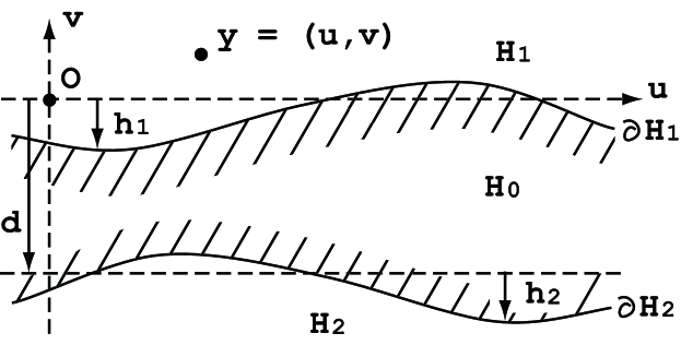
Figure 1. Region ${H}_{0}\subset\mathbb{R}^{m+1}$ is the shaded area between surfaces $\partial{H}_{1}$ and $\partial{H}_{2}$.

3. Frequentist measures of confidence for testing two regions

In this section, we review the multiscale bootstrap of Shimodaira (2008) for computing a frequentist $p$-value of “one-sided” test of ${H}_{0}^{\prime}$. Let $z=-\Phi^{-1}(\alpha)$ be the inverse function of $\alpha=\Phi(-z)$. The bootstrap $z$-value of ${H}_{0}^{\prime}$, defined as $z_{\sigma^{2}}({H}_{0}^{\prime}|y)=-\Phi^{-1}(\alpha_{\sigma^{2}}({H}_{0}^{\prime}|y))$, is convenient to work with. By multiplying $\sigma$ to it, $\sigma z_{\sigma^{2}}({H}_{0}^{\prime}|y)$ is called the normalized bootstrap $z$-value. Theorem 1 of Shimodaira (2008), as reproduced below, states that the $z$-value of $p({H}_{0}^{\prime}|y)$ is obtained by extrapolating the normalized bootstrap $z$-value to $\sigma^{2}=-1$, or equivalently $n^{\prime}=-n$ in terms of ${\cal X}^{*}$.

Theorem 1.

Let ${H}_{0}^{\prime}$ be a region of (10) with nearly flat $h_{1}$. Given ${H}_{0}^{\prime}$ and $y$, consider the normalized bootstrap $z$-value as a function of $\sigma^{2}$; We denote it by $\psi(\sigma^{2})=-\sigma\Phi^{-1}(\alpha_{\sigma^{2}}({H}_{0}^{\prime}|y))$. Let us define a frequentist $p$-value as

(11) $$p({H}_{0}^{\prime}|y)=\Phi(-\psi(-1)),$$

and assume that the right hand side exists. Then for $\mu\in\partial{H}_{0}^{\prime}$ and $0<\alpha<1$,

(12) $$P(p({H}_{0}^{\prime}|Y)<\alpha|\mu)=\alpha+O(\lambda^{3}),$$

meaning that the coverage error, i.e., the difference between the rejection probability and $\alpha$, vanishes asymptotically as $\lambda\to 0$, and that the $p$-value, or the associated hypothesis testing, is “similar on the boundary” asymptotically.

Proof

Here we show only an outline of the proof by allowing the coverage error of $O(\lambda^{2})$, instead of $O(\lambda^{3})$, in (12). This is a brief summary of the argument given in Shimodaira (2008). First define the expectation operator ${\cal E}_{\sigma^{2}}$ for a nearly flat function $h$ as

$$({\cal E}_{\sigma^{2}}h)(u):=E_{\sigma^{2}}(h(U^{*})|u),$$

where $E_{\sigma^{2}}(\cdot)$ on the right hand side denotes the expectation with respect to (7), that is, for $Y^{*}=(U^{*},V^{*})$ with

$$U^{*}|u\sim N_{m}(u,\sigma^{2}I_{m}),\quad V^{*}|v\sim N(v,\sigma^{2}).$$

Using the expectation operator, we next define two quantities

$$z_{1}=-\frac{v+{\cal E}_{\sigma^{2}}h_{1}(u)}{\sigma},\quad\epsilon_{1}=-\frac{h_{1}(U^{*})-{\cal E}_{\sigma^{2}}h_{1}(u)}{\sigma},$$

and work on the bootstrap probability as

(13) $$\alpha_{\sigma^{2}}({H}_{0}^{\prime}|y) = P_{\sigma^{2}}(V^{*}\leq-h_{1}(U^{*})|y)$$

$$= E_{\sigma^{2}}\left(\Phi(z_{1}+\epsilon_{1})|u\right)$$

$$= E_{\sigma^{2}}\left(\Phi(z_{1})+\phi(z_{1})\epsilon_{1}|u\right)+O(\lambda^{2})$$

$$= \Phi(z_{1})+O(\lambda^{2}).$$

The third equation is obtained by the Taylor series around $z_{1}$, and the last equation is obtained by $E_{\sigma^{2}}(\epsilon_{1}|u)=0$. Rearranging (13), we then get the scaling-law of the normalized bootstrap $z$-value as

(14) $$\psi(\sigma^{2})=v+{\cal E}_{\sigma^{2}}h_{1}(u)+O(\lambda^{2}).$$

On the other hand, eq. (5.10) of Shimodaira (2008) shows, by utilizing Fourier transforms of surfaces, that (12) holds with coverage error $O(\lambda^{2})$ for a $p$-value defined as

(15) $$p({H}_{0}^{\prime}|y)=\Phi(-v-{\cal E}_{-1}h_{1}(u))+O(\lambda^{2}).$$

The proof completes by combining (14) and (15). ∎

A hypothesis testing is to reject ${H}_{0}^{\prime}$ when observing $p({H}_{0}^{\prime}|y)<\alpha$ for a specified significance level, say, $\alpha=0.05$, and otherwise not to reject ${H}_{0}^{\prime}$. The left hand side of (12) is the rejection probability, which should be $\leq\alpha$ for $\mu\in{H}^{\prime}_{0}$ and $\geq\alpha$ for $\mu\not\in{H}^{\prime}_{0}$ to claim the unbiasedness of the test. On the other hand, the test is called similar on the boundary when the rejection probability is equal to $\alpha$ for $\mu\in\partial{H}_{0}^{\prime}$. In this paper, we implicitly assume that $p({H}_{0}^{\prime}|y)$ is decreasing as $y$ moves away from ${H}_{0}^{\prime}$. The rejection probability increases continuously as $\mu$ moves away from ${H}_{0}^{\prime}$. This assumption is justified when $\lambda$ is sufficiently small so that the behavior of $p({H}_{0}^{\prime}|y)$ is not very different from that for (2). Therefore, (12) implies that the $p$-value is approximately unbiased asymptotically as $\lambda\to 0$.

We can think of a procedure for calculating $p({H}_{0}^{\prime}|y)$ based on (11). In the procedure, the functional form of $\psi(\sigma^{2})$ should be estimated from the observed $\hat{\alpha}_{\sigma^{2}_{i}}$’s using parametric models. Then an approximately unbiased $p$-value is computed by extrapolating $\psi(\sigma^{2})$ to $\sigma^{2}=-1$. Our procedure works fine for the particular ${H}_{0}^{\prime}$ of (2), because $\psi(\sigma^{2})=y_{m+1}$ and $p({H}_{0}^{\prime}|y)=\Phi(-y_{m+1})=\Phi(-\psi(-1))$. Our procedure works fine also for any ${H}_{0}^{\prime}$ of (10) when the boundary surface $\partial{H}_{0}^{\prime}$ is smooth. The model is given as $\psi(\sigma^{2})=\beta_{0}+\beta_{1}\sigma^{2}+\beta_{2}\sigma^{4}+\beta_{3}\sigma^{6}+\cdots$ using parameters $\varphi=(\beta_{0},\beta_{1},\ldots)$, and thus an approximately unbiased $p$-value can be computed by $p({H}_{0}^{\prime}|y)=\Phi(-\hat{\beta}_{0}+\hat{\beta}_{1}-\hat{\beta}_{2}+\hat{\beta}_{3}-\cdots)$. It may be interesting to know that the parameters are interpreted as geometric quantities; $\beta_{0}$ is the distance from $y$ to the surface $\partial{H}_{0}^{\prime}$, $\beta_{1}$ is the mean curvature of the surface, and $\beta_{j}$, $j\geq 2$, is related to $2j$-th derivatives of $h_{1}$.

However, the series expansion above does not converge, i.e., $\psi(-1)$ does not exist, when $\partial{H}_{0}^{\prime}$ is nonsmooth. For example, $\psi(\sigma^{2})=\beta_{0}+\beta_{1}\sqrt{\sigma^{2}}$ serves as a good approximating model for cone-shaped ${H}_{0}^{\prime}$, for which $\psi(-1)$ does not take a value of $\mathbb{R}$. This observation agrees with the fact that an unbiased test does not exist for cone-shaped ${H}_{0}^{\prime}$ as indicated in the argument of Lehmann (1952). Instead of (11), the modified procedure of Shimodaira (2008) calculates a $p$-value defined as

(16) $$p_{k}({H}_{0}^{\prime}|y)=\Phi\left\{-\sum_{j=0}^{k-1}\frac{(-1-\sigma_{0}^{2})^{j}}{j!}\frac{\partial^{j}\psi(\sigma^{2})}{\partial(\sigma^{2})^{j}}\Bigr{|}_{\sigma_{0}^{2}}\right\}$$

for an integer $k>0$ and a real number $\sigma^{2}_{0}>0$. This is to extrapolate $\psi(\sigma^{2})$ back to $\sigma^{2}=-1$ by using the first $k$ terms of the Taylor series around $\sigma_{0}^{2}$. The coverage error in (12) should reduce as $k$ increases, but then the rejection region violates the desired property called monotonicity in the sense of Lehmann (1952) and Perlman and Wu (1999, 2003). For taking the balance, we chose $k=3$ and $\sigma_{0}^{2}=1$ for numerical examples in this paper.

4. Frequentist measures of confidence for testing three regions

The following theorem is our main result for computing a frequentist $p$-value of “two-sided” test of ${H}_{0}$. The proof is given in Appendix A.1.

Theorem 2.

Let ${H}_{0}$ be a region of (9) with nearly flat $h_{1}$ and $h_{2}$. Given ${H}_{0}$ and $y$, consider the approximately unbiased $p$-value $p({H}_{i}|y)$ by applying Theorem 1 to ${H}_{i}$ for $i=1,2$. Assuming these two $p$-values exist, let us define a frequentist $p$-value of ${H}_{0}$ as

(17) $$p({H}_{0}|y)=1-|p({H}_{1}|y)-p({H}_{2}|y)|.$$

For example, (17) holds for the exact $p$-value of (3) defined in Section 1. Then for $\mu\in\partial{H}_{0}=\partial{H}_{1}\cup\partial{H}_{2}$ and $0<\alpha<1$,

(18) $$P(p({H}_{0}|Y)<\alpha|\mu)=\alpha+O(\lambda^{2}),$$

meaning that $p({H}_{0}|y)$ is approximately unbiased asymptotically as $\lambda\to 0$.

For illustrating the methodology, let us work on the spherical shell example of Efron and Tibshirani (1998), for which we can still compute the exact $p$-values to verify our methods. The region of interest is ${H}_{0}:a_{2}\leq\|\mu\|\leq a_{1}$ as shown in Panel (a) of Fig. 2. We consider the case, say,

$$m+1=4,\quad a_{1}=6,\quad a_{2}=5,\quad\|y\|=5.9,$$

so that this region is analogous to (5) except for the curvature. The exact $p$-value for ${H}_{1}:\|\mu\|\geq a_{1}$ is easily calculated knowing that $\|Y\|^{2}$ is distributed as the chi-square distribution with degrees of freedom $m+1$ and noncentrality $\|\mu\|^{2}$. Writing this random variable as $\chi^{2}_{m+1}(\|\mu\|^{2})$, the exact $p$-value is $p({H}_{1}|y)=P(\chi^{2}_{m+1}(a_{1}^{2})\leq\|y\|^{2})=0.362$, that is, the probability of observing $\|Y\|\leq\|y\|$ for $\|\mu\|=a_{1}$. Similarly, the exact $p$-value for ${H}_{2}:\|\mu\|\leq a_{2}$ is $p({H}_{2}|y)=P(\chi^{2}_{m+1}(a_{2}^{2})\geq\|y\|^{2})=0.267$. In a similar way as for (3), the exact $p$-value for ${H}_{0}$ is computed numerically as $p({H}_{0}|y)=0.907$, although the procedure is a bit complicated as explained below. We first consider the critical constants $c_{1}$ and $c_{2}$ for the rejection regions ${R}_{1}=\{y\mid\|y\|<a_{1}-c_{1}\}$ and ${R}_{2}=\{y\mid\|y\|>a_{2}+c_{2}\}$. By equating the rejection probability to $\alpha$ for $\mu\in\partial{H}_{0}$, that is, $P(\chi^{2}_{m+1}(a_{i}^{2})<(a_{1}-c_{1})^{2})+P(\chi^{2}_{m+1}(a_{i}^{2})>(a_{2}+c_{2})^{2})=\alpha$ for $i=1,2$, we may get the solution numerically as $c_{1}=1.331$ and $c_{2}=1.903$ for $\alpha=0.05$, say. The $p$-value is defined as the infimum of $\alpha$ such that ${H}_{0}$ can be rejected.

To check if Theorem 2 is ever usable, we first compute (17) using the exact values of $p({H}_{1}|y)$ and $p({H}_{2}|y)$. Then we get $p({H}_{0}|y)=1-(0.362-0.267)=0.905$, which agrees extremely well to the exact $p({H}_{0}|y)=0.907$. The spherical shell is approximated by (9) only locally in a neighborhood of $y$ but not as a whole. Nevertheless, Theorem 2 worked fine.

We next think of the situation that bootstrap probabilities of ${H}_{1}$ and ${H}_{2}$ are available but not their exact $p$-values. We apply the procedure of Section 3 separately to the two regions for calculating the approximately unbiased $p$-values. To work on the procedure, here we consider a simple model $\psi(\sigma^{2})=\beta_{0}+\beta_{1}\sigma^{2}$ with parameters $\varphi=(\beta_{0},\beta_{1})$ for

(19) $$\alpha_{\sigma^{2}}({H}_{0}^{\prime}|y)=\Phi(-\psi(\sigma^{2})/\sigma).$$

Let $\psi_{i}(\sigma^{2})$ be the normalized bootstrap $z$-value of ${H}_{i}$ for $i=1,2$. By assuming the simple model for $\psi_{i}(\sigma^{2})$, we fit $\alpha_{\sigma^{2}}({H}_{i}|y)=\Phi(-\psi_{i}(\sigma^{2})/\sigma)$ to the observed multiscale bootstrap probabilities of ${H}_{i}$ for estimating the parameters. The actual estimation was done using the method described in Section 6.3, but we would like to forget the details for the moment. We get $\hat{\beta}_{0}=0.101$, $\hat{\beta}_{1}=-0.258$ for ${H}_{1}$, and similarly $\hat{\beta}_{0}=0.889$, $\hat{\beta}_{1}=0.286$ for ${H}_{2}$. $\beta_{0}$’s are interpreted as the distances from $y$ to the boundary surfaces, and the estimates agree well to the exact values $\beta_{0}=0.1$ for ${H}_{1}$ and $\beta_{0}=0.9$ for ${H}_{2}$. Then the approximately unbiased $p$-values are computed by (11) as $p({H}_{1}|y)=\Phi(-0.101-0.258)=0.360$ and $p({H}_{2}|y)=\Phi(-0.889+0.286)=0.273$, and thus (17) gives $p({H}_{0}|y)=1-(0.360-0.273)=0.913$, which again agrees well to the exact $p({H}_{0}|y)=0.907$.

We finally think of a more practical situation, where the bootstrap probabilities are not available for ${H}_{1}$ and ${H}_{2}$, but only for ${H}_{0}$. This situation is plausible in applications where many regions are involved and we are not sure which of them can be treated as ${H}_{1}$ or ${H}_{2}$ in a neighborhood of $y$; See Efron et al (1996) for an illustration. We consider a simple model $\psi_{1}(\sigma^{2})=\beta_{0}+\beta_{1}\sigma^{2}$, $\psi_{2}(\sigma^{2})=d-\beta_{0}-\beta_{1}\sigma^{2}$ with parameters $\varphi=(\beta_{0},\beta_{1},d)$ for

(20) $$\alpha_{\sigma^{2}}({H}_{0}|y)=1-(\Phi(-\psi_{1}(\sigma^{2})/\sigma)+\Phi(-\psi_{2}(\sigma^{2})/\sigma))$$

by assuming that the two surfaces are curved in the same direction with the same magnitude of curvature $|\beta_{1}|$. For estimating $\varphi$, (20) is fitted to the observed multiscale bootstrap probabilities of ${H}_{0}$ with constraints $\beta_{0}>-d/2$ and $d>0$, and $\hat{\varphi}$ is obtained as $\hat{\beta}_{0}=0.089$, $\hat{\beta}_{1}=-0.199$, $\hat{d}=0.995$. Then the approximately unbiased $p$-values are computed by (11) as $p({H}_{1}|y)=\Phi(-0.089-0.199)=0.387$ and $p({H}_{2}|y)=\Phi(-0.995+0.089+0.199)=0.240$ and thus (17) gives $p({H}_{0}|y)=1-(0.387-0.240)=0.853$. This is not very close to the exact $p({H}_{0}|y)=0.907$, partly because the model is too simple. However, it is a great improvement over $\alpha_{1}({H}_{0}|y)=P(a_{1}^{2}\leq\chi_{m+1}^{2}(\|y\|^{2})\leq a_{2}^{2})=0.320$.

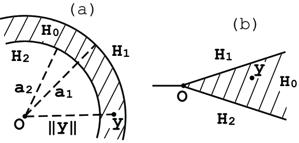
Figure 2. (a) Spherical shell region. (b) Cone-shaped region (Section 7).

5. Bayesian measures of confidence

Choosing a good prior density is essential for Bayesian inference. We consider a version of noninformative prior for making the posterior probability acquire frequentist properties.

First note that the sum of bootstrap probabilities of disjoint partitions of the whole parameter space is always 1. For the two regions case, $\alpha_{\sigma^{2}}({H}_{0}^{\prime}|y)+\alpha_{\sigma^{2}}({H}_{1}|y)=1$, and thus $\sigma z_{\sigma^{2}}({H}_{0}^{\prime}|y)+\sigma z_{\sigma^{2}}({H}_{1}|y)=0$. Therefore $p({H}_{0}^{\prime}|y)+p({H}_{1}|y)=1$ for the approximately unbiased $p$-values computed by (11), suggesting that we may think of a prior so that $p({H}_{0}^{\prime}|y)=\pi({H}_{0}^{\prime}|y)$. This was the idea of Efron and Tibshirani (1998) to define a Bayesian measure of confidence of ${H}_{0}$. Since each of ${H}_{1}$ and ${H}_{2}$ can be treated as ${H}_{0}^{\prime}$ by changing the coordinates, we may assume a prior satisfying

(21) $$\pi({H}_{i}|y)=p({H}_{i}|y),\quad i=1,2.$$

It follows from $\sum_{i=0}^{2}\pi({H}_{i}|y)=1$ that

(22) $$\pi({H}_{0}|y)=1-(p({H}_{1}|y)+p({H}_{2}|y)).$$

Priors satisfying (21) are called probability matching priors. The theory has been developed in literature (Peers, 1965; Tibshirani, 1989; Datta and Mukerjee, 2004) for posterior quantiles of a single parameter of interest. The examples are the flat prior $\pi(\mu)=$ const for the flat boundary case in Section 1, and $\pi(\mu)\propto\|\mu\|^{-m}$ for the spherical shell case in Section 4.

Our multiscale bootstrap method provides a new computation to $\pi({H}_{0}|y)$. We may simply compute (22) with the $p({H}_{1}|y)$ and $p({H}_{2}|y)$ used for computing $p({H}_{0}|y)$ of (17). Although we implicitly assumed the matching prior, we do not have to know the functional form of $\pi(\mu)$. For the spherical shell example, we may use the exact $p({H}_{1}|y)$ and $p({H}_{2}|y)$ to get $p({H}_{0}|y)=1-(0.362+0.267)=0.371$, or more practically, use only bootstrap probabilities of ${H}_{0}$ to get $p({H}_{0}|y)=1-(0.387+0.240)=0.373$.

6. Estimating parametric models for the scaling-law of bootstrap probabilities

6.1. One-step multiscale bootstrap

We first recall the estimation procedure of Shimodaira (2002, 2008) before describing our new proposals for improving the estimation accuracy in the following sections.

Let $f(\sigma^{2}|\varphi)$ be a parametric model of bootstrap probability such as (19) for ${H}_{0}^{\prime}$ or (20) for ${H}_{0}$. As already mentioned in Section 1, the model is fitted to the observed $C_{i}/B_{i}$, $i=1,\ldots,M$. Since $C_{i}$ is distributed as binomial with probability $f(\sigma_{i}^{2}|\varphi)$ and $B_{i}$ trials, the log-likelihood function is $\ell(\varphi)=\sum_{i=1}^{M}\{C_{i}\log f(\sigma_{i}^{2}|\varphi)+(B_{i}-C_{i})\log(1-f(\sigma_{i}^{2}|\varphi))\}$. The maximum likelihood estimate $\hat{\varphi}$ is computed numerically for each model. Let $\dim\varphi$ denote the number of parameters. Then $AIC=-2\ell(\hat{\varphi})+2\dim\varphi$ may be compared for selecting a best model among several candidate models.

6.2. Two-step multiscale bootstrap

Shimodaira (2004) has devised the multistep-multiscale bootstrap as a generalization of the multiscale bootstrap. The usual multiscale bootstrap is a special case called as the one-step multiscale bootstrap. Our new proposal here is to utilize the two-step multiscale bootstrap for improving the estimation accuracy of $\varphi$, although the two-step method was originally used for replacing the normal model of (1) with the exponential family of distributions.

Recalling that ${\cal X}^{*}$ is obtained by resampling from ${\cal X}$, we may resample again from ${\cal X}^{*}$, instead of ${\cal X}$, to get a bootstrap sample of size $n^{\prime\prime}$, and denote it as ${\cal X}^{**}=\{x^{**}_{1},\ldots,x^{**}_{n^{\prime\prime}}\}$. We formally consider the parametric bootstrap

$$Y^{**}|y^{*}\sim N_{m+1}(y^{*},(\tau^{2}-\sigma^{2})I_{m+1}),$$

where $\tau$ is a new scale defined by $\tau^{2}-\sigma^{2}=n/n^{\prime\prime}$. In Shimodaira (2004), only the marginal distribution $Y^{**}|y\sim N_{m+1}(y,\tau^{2}I_{m+1})$ is considered to detect the nonnormality. For the second step, $P_{\sigma^{2},\tau^{2}}(Y^{**}\in{H}_{0}|y)=\alpha_{\tau^{2}}({H}_{0}|y)$ should have the same functional form as $P_{\sigma^{2},\tau^{2}}(Y^{*}\in{H}_{0}|y)=\alpha_{\sigma^{2}}({H}_{0}|y)$ for the normal model. Here we also consider the joint distribution of $(Y^{*},Y^{**})$ given $y$. It is $2m+2$-dimensional multivariate normal with $Cov(Y^{*},Y^{**}|y)=\sigma^{2}I_{m+1}$. We denote the probability and the expectation by $P_{\sigma^{2},\tau^{2}}(\cdot|y)$ and $E_{\sigma^{2},\tau^{2}}(\cdot|y)$, respectively. Then, the joint bootstrap probability is defined as

$$\alpha_{\sigma^{2},\tau^{2}}({H}_{0}|y)=P_{\sigma^{2},\tau^{2}}(Y^{*}\in{H}_{0}\wedge Y^{**}\in{H}_{0}|y).$$

Let $g(\sigma^{2},\tau^{2}|\varphi)$ be a parametric model of $\alpha_{\sigma^{2},\tau^{2}}({H}_{0}^{\prime}|y)$ or $\alpha_{\sigma^{2},\tau^{2}}({H}_{0}|y)$. To work on specific forms of $g(\sigma^{2},\tau^{2}|\varphi)$, we need some notations. Let $(X^{\prime},X^{\prime\prime})$ be distributed as bivariate normal with mean $(0,0)$, variance $V(X^{\prime})=V(X^{\prime\prime})=1$, and covariance $Cov(X^{\prime},X^{\prime\prime})=\rho$. The distribution function is denoted as $\Phi_{\rho}(a_{1},b_{1})=P(X^{\prime}\leq a_{1}\wedge X^{\prime\prime}\leq b_{1})$, where the joint density is explicitly given as $\phi_{\rho}(a_{1},b_{1})=(1-\rho^{2})^{-1/2}\phi((1-\rho^{2})^{-1/2}(b_{1}-\rho a_{1}))\phi(a_{1})$. We also define $\Phi_{\rho}(a_{1},b_{1};a_{2},b_{2})=P(a_{2}\leq X^{\prime}\leq a_{1}\wedge b_{2}\leq X^{\prime\prime}\leq b_{1})=\Phi_{\rho}(a_{1},b_{1})-\Phi_{\rho}(a_{2},b_{1})-\Phi_{\rho}(a_{1},b_{2})+\Phi(a_{2},b_{2})$. Then a generalization of (14) is given as follows. The proof is in Appendix A.2.

Lemma 1.

For sufficiently small $\lambda$, the joint bootstrap probabilities for ${H}_{0}^{\prime}$ and ${H}_{0}$ are expressed asymptotically as

(23) $$\alpha_{\sigma^{2},\tau^{2}}({H}^{\prime}_{0}|y) = \Phi_{\rho}(z_{1},w_{1})+O(\lambda^{2}),$$

(24) $$\alpha_{\sigma^{2},\tau^{2}}({H}_{0}|y) = \Phi_{\rho}(z_{1},w_{1};z_{2},w_{2})+O(\lambda^{2}),$$

where $z_{1}=-(v+{\cal E}_{\sigma^{2}}h_{1}(u))/\sigma$, $w_{1}=-(v+{\cal E}_{\tau^{2}}h_{1}(u))/\tau$, $z_{2}=-(v+d+{\cal E}_{\sigma^{2}}h_{2}(u))/\sigma$, $w_{2}=-(v+d+{\cal E}_{\tau^{2}}h_{2}(u))/\tau$, and $\rho=\sigma/\tau$.

Thus $g(\sigma^{2},\tau^{2}|\varphi)$ is specified for ${H}_{0}^{\prime}$ as (23) with $z_{1}=-\psi(\sigma^{2})/\sigma$, $w_{1}=-\psi(\tau^{2})/\tau$ using the $\psi$ function of (19). Similarly, $g(\sigma^{2},\tau^{2}|\varphi)$ is specified for ${H}_{0}$ as (24) with $z_{1}=\psi_{1}(\sigma^{2})/\sigma$, $w_{1}=\psi_{1}(\tau^{2})/\tau$, $z_{2}=-\psi_{2}(\sigma^{2})/\sigma$, $w_{2}=-\psi_{2}(\tau^{2})/\tau$ using $\psi_{1}$ and $\psi_{2}$ functions of (20).

We may specify $M$ sets of $(\sigma,\tau)$, denoted as $(\sigma_{1},\tau_{1}),\ldots,(\sigma_{M},\tau_{M})$. In our numerical examples, $\sigma_{1},\ldots,\sigma_{13}$ are specified as mentioned in Section 1 and $\tau_{i}$’s are specified so that $\tau_{i}^{2}-\sigma_{i}^{2}=1$ holds always, meaning $n^{\prime\prime}=n$. For each $i=1,\ldots,M$, we generate $(Y^{*},Y^{**})$ with $(\sigma_{i},\tau_{i})$ many times, say $B_{i}=10000$, and observe the frequencies $C_{i}=\#(Y^{*}\in{H}_{0})$, $D_{i}=\#(Y^{**}\in{H}_{0})$, and $E_{i}=\#(Y^{*}\in{H}_{0}\wedge Y^{**}\in{H}_{0})$. Note that only one $Y^{**}$ is generated from each $Y^{*}$ here, whereas thousands of $Y^{**}$’s may be generated from each $Y^{*}$ in the double bootstrap method. The log-likelihood function becomes $\ell(\varphi)=\sum_{i=1}^{M}\{E_{i}\log g(\sigma^{2}_{i},\tau^{2}_{i}|\varphi)+(C_{i}-E_{i})\log(f(\sigma^{2}_{i}|\varphi)-g(\sigma^{2}_{i},\tau^{2}_{i}|\varphi))+(D_{i}-E_{i})\log(f(\tau^{2}_{i}|\varphi)-g(\sigma^{2}_{i},\tau^{2}_{i}|\varphi))+(B_{i}-C_{i}-D_{i}+E_{i})\log(1-f(\sigma^{2}_{i}|\varphi)-f(\tau^{2}_{i}|\varphi)+g(\sigma^{2}_{i},\tau^{2}_{i}|\varphi))\}$. In fact, we have used this two-step multiscale bootstrap, instead of the one-step method, in all the numerical examples.

The one-step method had difficulty in distinguishing ${H}_{0}$ with very small $d$ from ${H}_{0}$ with moderate $d$ but heavily curved $\partial{H}_{1}$. The two-step method avoids this identifiability issue because a small value of $E_{i}$ indicates that $d$ is small; It is automatically done, of course, by the numerical optimization of $\ell(\varphi)$.

6.3. Higher-order terms of bootstrap probabilities for testing two regions

The asymptotic errors of the scaling law of the bootstrap probabilities in (13) and (23) are of order $O(\lambda^{2})$. As shown in the following lemma, the errors can be reduced to $O(\lambda^{3})$ by introducing correction terms of $O(\lambda^{2})$ for improving the parametric model $g(\sigma^{2},\tau^{2}|\varphi)$ of ${H}_{0}^{\prime}$. The proof is given in Appendix A.3.

Lemma 2.

For sufficiently small $\lambda$, the bootstrap probabilities for ${H}_{0}^{\prime}$ are expressed asymptotically as

(25) $$\alpha_{\sigma^{2}}({H}_{0}^{\prime}|y) = \Phi(z_{1}+\Delta z_{1})+O(\lambda^{3})$$

(26) $$\alpha_{\tau^{2}}({H}_{0}^{\prime}|y) = \Phi(w_{1}+\Delta w_{1})+O(\lambda^{3})$$

(27) $$\alpha_{\sigma^{2},\tau^{2}}({H}^{\prime}_{0}|y) = \Phi_{\rho+\Delta\rho}(z_{1}+\Delta z_{1},w_{1}+\Delta w_{1})+O(\lambda^{3}),$$

where $z_{1}$, $w_{1}$, and $\rho$ are those defined in Lemma 1, and the higher order correction terms are defined as $\Delta z_{1}=-\frac{1}{2}z_{1}E_{\sigma^{2},\tau^{2}}(\epsilon_{1}^{2}|u)$, $\Delta w_{1}=-\frac{1}{2}w_{1}E_{\sigma^{2},\tau^{2}}(\delta_{1}^{2}|u)$, and $\Delta\rho=-\frac{1}{2}\left(\rho E_{\sigma^{2},\tau^{2}}(\epsilon_{1}^{2}|u)+\rho E_{\sigma^{2},\tau^{2}}(\delta_{1}^{2}|u)-2E_{\sigma^{2},\tau^{2}}(\epsilon_{1}\delta_{1}|u)\right)$ using

(28) $$\epsilon_{1}=-\frac{h_{1}(U^{*})-{\cal E}_{\sigma^{2}}h_{1}(u)}{\sigma},\quad\delta_{1}=-\frac{h_{1}(U^{**})-{\cal E}_{\tau^{2}}h_{1}(u)}{\tau}.$$

For deriving a very simple model for $\Delta\rho$, we think of a situation $h(u)=(A/\!\sqrt{m})\|u\|+(B/m)\|u\|^{2}$ and $\theta=0$, and consider asymptotics as $m\to\infty$. This formulation is only for convenience of derivation. The two values $A$ and $B$ will be specified later by looking at the functional form of $f(\sigma^{2}|\varphi)$. A straightforward, yet tedious, calculation (the details are not shown) gives $\psi(\sigma^{2})=\mbox{const}+A\sigma+B\sigma^{2}+O(m^{-1})$ and

$$\Delta\rho=-\frac{1}{2m}\left(A^{2}\rho(1-\rho)+2B^{2}\rho(\tau^{2}-\sigma^{2})+2AB\sigma(1-\rho^{2})\right)+O(m^{-3/2}).$$

This correction term was in fact already used for the simple model $\psi(\sigma^{2})=\beta_{0}+\beta_{1}\sigma^{2}$ of the spherical shell example in Section 4, where the parameter was actually $\varphi=(\beta_{0},\beta_{1},m)$ instead of $\varphi=(\beta_{0},\beta_{1})$. We did not change the $\psi(\sigma^{2})$ for adjusting $\Delta z_{1}$ and $\Delta w_{1}$, meaning that $z_{1}+\Delta z_{1}$, instead of $z_{1}$, was modelled as $-\psi(\sigma^{2})/\sigma$. Comparing the coefficients of $\psi(\sigma^{2})$, we get $A=0$ and $B=\beta_{1}$, and thus $\Delta\rho=-(\beta_{1})^{2}(\sigma/\tau)(\tau^{2}-\sigma^{2})/m$. When (19) was fitted to ${H}_{1}$, the estimated parameter $\hat{m}=2.83$ was close to the true value $m=3$.

For the numerical example mentioned above, we have also fitted the same model but $\Delta\rho=0$ being fixed. The estimated parameters are $\hat{\beta}_{0}=0.101$, $\hat{\beta}_{1}=-0.256$, and the $p$-value is $p({H}_{1}|y)=\Phi(-0.101-0.256)=0.361$. These values are not much different from those shown in Section 4. However, the AIC value improved greatly by the introduction of $\Delta\rho$, and the AIC difference was 96.67, mostly because improved fitting for the joint bootstrap probability of (27). My experience suggests that consideration of the $\Delta\rho$ term is useful for choosing a reasonable model of $\psi(\sigma^{2})$.

7. Simulation study

Let us consider a cone-shaped region ${H}_{0}$ in $\mathbb{R}^{2}$ with the angle at the vertex being $2\pi/10$ as shown in Panel (b) of Fig. 2. This cone can be regarded, locally in a neighborhood of $y$ with appropriate coordinates, as ${H}_{0}$ of (9) when $y$ is close to one of the edges but far from the vertex, or as ${H}_{0}^{\prime}$ of (10) when $y$ is close to the vertex. In this section, the cone is labelled either by ${H}_{0}$ or ${H}_{0}^{\prime}$ depending on which view we are taking.

Cones in $\mathbb{R}^{2}$ appear in the problem of multiple comparisons of three elements $X_{0},X_{1},X_{2}$, say, and ${H}_{i}$ corresponds to the hypothesis that the mean of $X_{i}$ is the largest among the three (DuPreez et al, 1985; Perlman and Wu, 2003; Shimodaira, 2008). The angle at the vertex is related to the covariance structure of the elements. Although an unbiased test does not exist for this region, we would like to see how our methods work for reducing the coverage error.

Contour lines of confidence measures, denoted $p(y)$ in general, at the levels 0.05 and 0.95 are drawn in Fig. 3. The rejection regions of the cone and the complement of the cone are ${R}=\{y|p(y)<0.05\}$ and ${R}^{\prime}=\{y|p(y)>0.95\}$, respectively, at $\alpha=0.05$. We observe that $p(y)$ decreases as $y$ moves away from the cone in Panels (a), (b), and (c); See Appendix B for the details of computation. On the other hand, Figs. 4 and 5 show the rejection probability. For an unbiased test, it should be 5% for all the $\mu\in\partial{H}_{0}$ so that the coverage error is zero.

In Panel (a) of Fig. 3, $p(y)=\alpha_{1}({H}_{0}|y)$ is computed by the bootstrap samples of $\sigma^{2}=1$. This bootstrap probability, labelled as BP in Fig. 4, is heavily biased near the vertex, and this tendency is enhanced when the angle becomes $2\pi/20$ in Fig. 5.

In Panel (b) of Fig. 3, $p(y)=p({H}_{0}^{\prime}|y)$ is computed by regarding the cone as ${H}_{0}^{\prime}$ of (10). The dent of ${R}$ and the bump of ${R}^{\prime}$ become larger than those of Panel (a) of Fig. 3 near the vertex, confirming what we observed in Shimodaira (2008). As seen in Figs. 4 and 5, the coverage error of $p({H}_{0}^{\prime}|y)$, labelled as “one sided” there, is smaller than that of BP.

In Panel (c) of Fig. 3, $p({H}_{0}|y)$ is also computed by regarding the cone as ${H}_{0}$ of (9), and then one of $p({H}_{0}^{\prime}|y)$ and $p({H}_{0}|y)$ is selected as $p(y)$ by comparing the AIC values at each $y$. This $p(y)$, labelled as “two sided Freq” in Figs. 4 and 5, improves greatly on the one-sided $p$-value. The coverage error is almost zero except for small $\|\mu\|$’s, verifying what we attempted in this paper. The corresponding Bayesian posterior probability, labelled as “two sided Bayes,” performs similarly. Note that the coverage error was further reduced near the vertex by setting simply $p(y)=p({H}_{0}|y)$ without the model selection (the result is not shown here); However, the shapes of $R$ and ${R}^{\prime}$ became rather weird then in the sense mentioned at the last paragraph of Section 3.

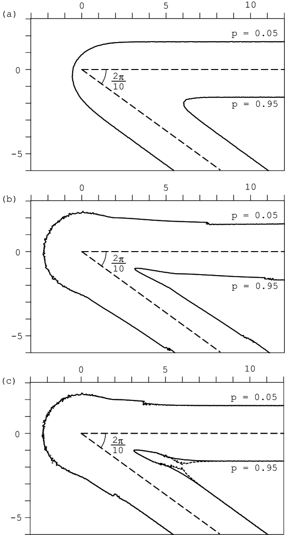
Figure 3. Contour lines $p(y)=0.05$ and $p(y)=0.95$. The cone-shaped region ${H}_{0}$ is rotated so that one of the edges is placed along the x-axis. Solid curves are drawn for (a) the bootstrap probability with $\sigma^{2}=1$, and for (b) the frequentist $p$-value for “one-sided” test. In Panel (c), $p(y)$ is switched to the frequentist $p$-value for “two-sided” test when appropriate. The dotted curve in Panel (c) is for the Bayesian posterior probability.

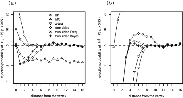
Figure 4. (a) Rejection probability of the cone, and (b) that of the complement of the cone. The angle at the vertex is $2\pi/10$.

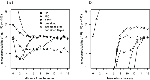
Figure 5. (a) Rejection probability of the cone, and (b) that of the complement of the cone. The angle at the vertex is $2\pi/20$.

8. Concluding Remarks

In this paper, we have discussed frequentist and Bayesian measures of confidence for the three regions case, and have proposed a new computation method using the multiscale bootstrap technique. In this method, AIC played an important role for choosing appropriate parametric models of the scaling-law of bootstrap probability. Simulation study showed that the proposed frequentist measure performs better for controlling the coverage error than the previously proposed multiscale bootstrap designed only for the two regions case.

A generalization of the confidence measures gives a frequentist interpretation of the Bayesian posterior probability as follows. Let us consider the situation of Theorem 2. If we strongly believe that $\mu\not\in{H_{2}}$, we could use the one-sided $p$-value $p({H}_{0}^{\prime}|y)=1-p({H}_{1}|y)$, instead of the two sided $p({H}_{0}|y)$. Similarly, we might use $1-p({H}_{2}|y)$ if we believe that $\mu\not\in{H}_{1}$. By making the choice “adaptively,” someone may want to use $p^{(1)}({H}_{0}|y)=1-\max(p({H}_{1}|y),p({H}_{2}|y))$, although it is not justified in terms of coverage error. By connecting $p^{(1)}({H}_{0}|y)$ and $p({H}_{0}|y)$ linearly using an index $s$ for the number of “sides,” we get

$$p^{(s)}({H}_{0}|y)=\pi({H}_{0}|y)+s\min(p({H}_{1}|y),p({H}_{2}|y)).$$

It is easily verified that $p({H}_{0}|y)=p^{(2)}({H}_{0}|y)$ and $\pi({H}_{0}|y)=p^{(0)}({H}_{0}|y)$, indicating that the Bayesian posterior probability defined in Section 5 can be interpreted, interestingly, as a frequentist $p$-value of “zero-sided” test of ${H}_{0}$. Although we have no further consideration, this kind of argument might lead to yet another compromise between frequentist and Bayesian.

Our formulation is rather restrictive. We have considered only the three regions case by introducing the surface $h_{2}$ in addition to the surface $h_{1}$ of the two regions case. Also these two surfaces are assumed to be nearly parallel to each other. It is worth to elaborate on generalizations of this formulation in future work, but too much of complication may result in unstable computation for estimating the scaling-law of bootstrap probability. AIC will be useful again in such a situation.

Appendix A Proofs

A.1. Proof of Theorem 2

First we consider rejection regions of testing ${H}_{0}$ for a specified $\alpha$ by modifying the two rejection regions of (3). Since $h_{1}$ and $h_{2}$ are nearly flat, the modified regions should be expressed as ${R}_{1}=\{(u,v)\mid v>c-r_{1}(u),\,u\in\mathbb{R}^{m}\}$ and ${R}_{2}=\{(u,v)\mid v<-d-c-r_{2}(u),\,u\in\mathbb{R}^{m}\}$ using nearly flat functions $r_{1}$ and $r_{2}$. The constant $c$ is the same one as defined in (4). Write $a=\phi(c)$, $b=\phi(c+d)$ for brevity sake. We evaluate the rejection probability for $\mu\in\partial{H}_{1}\cup\partial{H}_{2}$. Let $\mu\in\partial{H}_{1}$ for a moment, and put $\mu=(\theta,-h_{1}(\theta))$. By applying the argument of (13) to ${R}_{1}$ but (7) is replaced by (1), we get $P(Y\in{R}_{1}|\mu)=1-\Phi(c-{\cal E}_{1}r_{1}(\theta)+h_{1}(\theta))+O(\lambda^{2})=\Phi(-c)+a({\cal E}_{1}r_{1}(\theta)-h_{1}(\theta))+O(\lambda^{2})$. The same argument applied to ${R}_{2}$ gives $P(Y\in{R}_{2}|\mu)=\Phi(-d-c-{\cal E}_{1}r_{2}(\theta)+h_{1}(\theta))+O(\lambda^{2})=\Phi(-d-c)+b(-{\cal E}_{1}r_{2}(\theta)+h_{1}(\theta))+O(\lambda^{2})$. Rearranging these two formula with the identity

(29) $$P(Y\in{R}_{1}|\mu)+P(Y\in{R}_{2}|\mu)=\alpha$$

for an unbiased test, we get an equation $a({\cal E}_{1}r_{1}(\theta)-h_{1}(\theta))+b(-{\cal E}_{1}r_{2}(\theta)+h_{1}(\theta))=O(\lambda^{2})$. By exchanging the roles of $r_{1}$ and $r_{2}$, the equation becomes $b({\cal E}_{1}r_{1}(\theta)-h_{2}(\theta))+a(-{\cal E}_{1}r_{2}(\theta)+h_{2}(\theta))=O(\lambda^{2})$ for $\mu\in\partial{H}_{2}$ with $\mu=(\theta,-d-h_{2}(\theta))$. These two equations are expressed as

(30) $$\left(\begin{array}[]{cc}a&-b\\ -b&a\end{array}\right)\left(\begin{array}[]{c}{\cal E}_{1}r_{1}(\theta)\\ {\cal E}_{1}r_{2}(\theta)\end{array}\right)=(a-b)\left(\begin{array}[]{c}h_{1}(\theta)\\ h_{2}(\theta)\end{array}\right)+O(\lambda^{2}).$$

For solving this equation with respect to $r_{1}$ and $r_{2}$, first apply the inverse matrix of the $2\times 2$ matrix from the left in (30), and then apply the inverse operator of ${\cal E}_{1}$ so that

(31) $$\left(\begin{array}[]{c}r_{1}(u)\\ r_{2}(u)\end{array}\right)=\frac{1}{a+b}\left(\begin{array}[]{cc}a&b\\ b&a\end{array}\right)\left(\begin{array}[]{c}{\cal E}_{-1}h_{1}(u)\\ {\cal E}_{-1}h_{2}(u)\end{array}\right)+O(\lambda^{2}).$$

Next we obtain an expression of $p$-value corresponding to the rejection regions. $p({H}_{0}|y)$ is defined as the value of $\alpha$ for which either of $y\in\partial{R}_{1}$ and $y\in\partial{R}_{2}$ holds. Note that $r_{1}$, $r_{2}$, and $c$ depend on $\alpha$. Let us assume $y\in\partial{R}_{1}$ and thus $c=v+r_{1}(u)$ for a moment. Write $a^{\prime}=\phi(v)=a+O(\lambda)$, $b^{\prime}=\phi(v+d)=b+O(\lambda)$ for brevity sake. Recalling (4), $p({H}_{0}|y)=\Phi(-c)+\Phi(-d-c)=\Phi(-v-r_{1}(u))+\Phi(-d-v-r_{1}(u))=\Phi(-v)+\Phi(-d-v)-(a^{\prime}+b^{\prime})r_{1}(u)+O(\lambda^{2})$, where $r_{1}(u)$ in (31) can be expressed as

$$r_{1}(u)=\frac{a^{\prime}}{a^{\prime}+b^{\prime}}{\cal E}_{-1}h_{1}(u)+\frac{b^{\prime}}{a^{\prime}+b^{\prime}}{\cal E}_{-1}h_{2}(u)+O(\lambda^{2}).$$

Therefore, $p({H}_{0}|y)=\Phi(-v)+\Phi(-d-v)-a^{\prime}{\cal E}_{-1}h_{1}(u)-b^{\prime}{\cal E}_{-1}h_{2}(u)+O(\lambda^{2})=\Phi(-v-{\cal E}_{-1}h_{1}(u))+\Phi(-d-v-{\cal E}_{-1}h_{2}(u))+O(\lambda^{2})$. By applying (15) to ${H}_{1}$ and ${H}_{2}$, respectively, we get $p({H}_{1}|y)=\Phi(v+{\cal E}_{-1}h_{1}(u))+O(\lambda^{2})$ and $p({H}_{2}|y)=\Phi(-v-d-{\cal E}_{-1}h_{2}(u))+O(\lambda^{2})$, and thus $p({H}_{0}|y)=1-p({H}_{1}|y)+p({H}_{2}|y)+O(\lambda^{2})$. By exchanging the roles of ${H}_{1}$ and ${H}_{2}$, we have $p({H}_{0}|y)=1-p({H}_{2}|y)+p({H}_{1}|y)+O(\lambda^{2})$ for $y\in\partial{R}_{2}$. By taking the minimum of these two expressions of $p({H}_{0}|y)$, we finally obtain (17). This $p$-value satisfies (29) with error $O(\lambda^{2})$, and thus (18) holds.

A.2. Proof of Lemma 1

The argument is very similar to (13) in the proof of Theorem 1. Given $v,u^{*},u^{**}$, the joint distribution of $X^{\prime}=(V^{*}-v)/\sigma$ and $X^{\prime\prime}=(V^{**}-v)/\tau$ is $\Phi_{\rho}$. Therefore, $P_{\sigma^{2},\tau^{2}}(V^{*}\leq-h_{1}(u^{*})\wedge V^{**}\leq-h_{1}(u^{**})|v,u^{*},u^{**})=P_{\sigma^{2},\tau^{2}}(X^{\prime}\leq z_{1}+\epsilon_{1}\wedge X^{\prime\prime}\leq w_{1}+\delta_{1}|v,u^{*},u^{**})=\Phi_{\rho}(z_{1}+\epsilon_{1},w_{1}+\delta_{1})$, where $\epsilon_{1}$ and $\delta_{1}$ are defined in (28). Taking the expectation with respect to $(U^{*},U^{**})$, we have $\alpha_{\sigma^{2},\tau^{2}}({H}^{\prime}_{0}|y)=P_{\sigma^{2},\tau^{2}}(V^{*}\leq-h_{1}(U^{*})\wedge V^{**}\leq-h_{1}(U^{**})|y)=E_{\sigma^{2},\tau^{2}}(\Phi_{\rho}(z_{1}+\epsilon_{1},w_{1}+\delta_{1})|u)$. For proving (23), considering the Taylor series around $(z_{1},w_{1})$, we obtain

(32) $$E_{\sigma^{2},\tau^{2}}\left(\Phi_{\rho}(z_{1},w_{1})+\frac{\partial\Phi_{\rho}}{\partial z_{1}}\epsilon_{1}+\frac{\partial\Phi_{\rho}}{\partial w_{1}}\delta_{1}\big{|}u\right)+O(\lambda^{2})$$

with $E_{\sigma^{2},\tau^{2}}(\epsilon_{1}|u)=E_{\sigma^{2},\tau^{2}}(\delta_{1}|u)=0$ for completing the proof.

Next we show (24). The conditional probability given $v,u^{*},u^{**}$ is $P_{\sigma^{2},\tau^{2}}(-d-h_{2}(u^{*})\leq V^{*}\leq-h_{1}(u^{*})\wedge-d-h_{2}(u^{**})\leq V^{**}\leq-h_{1}(u^{**})|v,u^{*},u^{**})=P_{\sigma^{2},\tau^{2}}(z_{2}+\epsilon_{2}\leq X^{\prime}\leq z_{1}+\epsilon_{1}\wedge w_{2}+\delta_{2}\leq X^{\prime\prime}\leq w_{1}+\delta_{1}|v,u^{*},u^{**})=\Phi_{\rho}(z_{1}+\epsilon_{1},w_{1}+\delta_{1};z_{2}+\epsilon_{2},w_{2}+\delta_{2})$, where

$$\epsilon_{2}=-\frac{h_{2}(U^{*})-{\cal E}_{\sigma^{2}}h_{2}(u)}{\sigma},\quad\delta_{2}=-\frac{h_{2}(U^{**})-{\cal E}_{\tau^{2}}h_{2}(u)}{\tau}.$$

Taking the expectation with respect to $(U^{*},U^{**})$, we have $\alpha_{\sigma^{2},\tau^{2}}({H}_{0}|y)=P_{\sigma^{2},\tau^{2}}(-d-h_{2}(U^{*})\leq V^{*}\leq-h_{1}(U^{*})\wedge-d-h_{2}(U^{**})\leq V^{**}\leq-h_{1}(U^{**})|y)=E_{\sigma^{2},\tau^{2}}(\Phi_{\rho}(z_{1}+\epsilon_{1},w_{1}+\delta_{1};z_{2}+\epsilon_{2},w_{2}+\delta_{2})|u)$. We only have to consider the Taylor series

$$E_{\sigma^{2},\tau^{2}}\left(\Phi_{\rho}(z_{1},w_{1};z_{2},w_{2})+\frac{\partial\Phi_{\rho}}{\partial z_{1}}\epsilon_{1}+\frac{\partial\Phi_{\rho}}{\partial w_{1}}\delta_{1}+\frac{\partial\Phi_{\rho}}{\partial z_{2}}\epsilon_{2}+\frac{\partial\Phi_{\rho}}{\partial w_{2}}\delta_{2}\big{|}u\right)+O(\lambda^{2})$$

with $E_{\sigma^{2},\tau^{2}}(\epsilon_{i}|u)=E_{\sigma^{2},\tau^{2}}(\delta_{i}|u)=0$, $i=1,2$ for completing the proof.

A.3. Proof of Lemma 2

By considering a higher-order term of the Taylor series in (13), we obtain $\alpha_{\sigma^{2}}({H}_{0}^{\prime}|y)=E_{\sigma^{2}}(\Phi(z_{1})+\phi(z_{1})\epsilon_{1}-\phi(z_{1})z_{1}\epsilon_{1}^{2}/2|u)+O(\lambda^{3})=\Phi(z_{1})+\phi(z_{1})\Delta z_{1}+O(\lambda^{3})=\Phi(z_{1}+\Delta z_{1})+O(\lambda^{3})$, proving (25) as well as (26). On the other hand, (27) is shown by considering higher-order terms of the Taylor series in (32) as

$$E_{\sigma^{2},\tau^{2}}\Bigl{(}\Phi_{\rho}(z_{1},w_{1}) + \frac{\partial\Phi_{\rho}}{\partial z_{1}}\epsilon_{1}+\frac{\partial\Phi_{\rho}}{\partial w_{1}}\delta_{1}$$

$$+ \frac{1}{2}\Bigl{(}\frac{\partial^{2}\Phi_{\rho}}{\partial z_{1}^{2}}\epsilon_{1}^{2}+2\frac{\partial^{2}\Phi_{\rho}}{\partial z_{1}\partial w_{1}}\epsilon_{1}\delta_{1}+\frac{\partial^{2}\Phi_{\rho}}{\partial w_{1}^{2}}\delta_{1}^{2}\Bigr{)}\big{|}u\Bigr{)}+O(\lambda^{3}).$$

The proof completes by rearranging the above formula with

$$\frac{\partial^{2}\Phi_{\rho}}{\partial z_{1}^{2}}=-z_{1}\frac{\partial\Phi_{\rho}}{\partial z_{1}}-\rho\phi_{\rho}(z_{1},w_{1}),\quad\frac{\partial^{2}\Phi_{\rho}}{\partial z_{1}\partial w_{1}}=\phi_{\rho}(z_{1},w_{1}),\quad\frac{\partial\Phi_{\rho}}{\partial\rho}=\phi_{\rho}(z_{1},w_{1}).$$

Appendix B Simulation Details

The contour lines in Fig. 3 are drawn by computing $p$-values at all grid points ($300\times 180$) of step size 0.05 in the rectangle area; This huge computation was made possible by parallel processing using up to 700 cpus. The computation takes a few minutes per each grid point per cpu. Our algorithm is implemented as an experimental version of the scaleboot package of Shimodaira (2006), which will be included soon in the release version available from CRAN.

The rejection probabilities in Figs. 4 and 5 are computed by generating $y$ according to (1) for 10000 times, and then counting how many times $p(y)<0.05$ or $p(y)>0.95$ is observed. This computation is done for each $\mu\in\partial{H}_{0}$ with the distance from the vertex $\|\mu\|=0,1,\ldots,16$, i.e., $\mu=(0,0),(1,0),\ldots,(16,0)$ in the coordinates of Fig. 3.

For computing $p({H}^{\prime}_{0}|y)$ and $p({H}_{0}|y)$, the two-step multiscale bootstrap described in Section 6.2 was performed with the $M=13$ sets of scales $(\sigma_{i},\tau_{i})$, $i=1,\ldots,13$, specified there. The parametric bootstrap, instead of the resampling, was used for the simulation. The number of bootstrap samples has increased to $B_{i}=10^{5}$ for making the contour lines smoother, while it was $B_{i}=10^{4}$ in the other results.

For $p({H}^{\prime}_{0}|y)$, we have considered the singular model of Shimodaira (2008) defined as $\psi(\sigma^{2})=\beta_{0}+\beta_{1}/(1+\beta_{2}(\sigma-1))$ for cones, and performed the model fitting method described in Section 6.3. From the Taylor series of this $\psi(\sigma^{2})$ around $\sigma=1$, we get $A=\beta_{1}\beta_{2}(3-2\beta_{2})$, $B=\beta_{1}(\beta_{2}-1)^{2}$ for computing the higher order correction term $\Delta\rho$. We have also considered submodels by restricting some of $\varphi=(\beta_{0},\beta_{1},\beta_{2},m)$ to specified values, and the minimum AIC model is chosen at each $y$. The frequentist $p$-value is computed by (16) with $k=3$ and $\sigma_{0}^{2}=1$.

For $p({H}_{0}|y)$, we have considered the same singular model for the two surfaces by assuming they are curved in the opposite directions with the same magnitude of curvature. More specifically, the two $\psi$ functions in (20) are defined as $\psi_{1}(\sigma^{2})=\beta_{0}+\beta_{1}/(1+\beta_{2}(\sigma-1))$ and $\psi_{2}(\sigma^{2})=d-\beta_{0}+\beta_{1}/(1+\beta_{2}(\sigma-1))$. The parameters $\varphi=(\beta_{0},\beta_{1},\beta_{2},d)$ are estimated by the model fitting method described in Section 6.2. Submodels are also considered and model selection is performed using AIC. The frequentist $p$-value is computed by (17), and the Bayesian posterior probability is computed by (22).

The rejection probabilities of other two commonly used measures are shown only for reference purposes; See Shimodaira (2008) for the details. The rejection probability of the multiple comparisons, denoted MC here, is always below 5% in Panel (a), and the coverage error becomes zero at the vertex. On the other hand, the rejection probability of the $z$-test is always below 5% in Panel (b), and the coverage error reduces to zero as $\|\mu\|\to\infty$.

References

• Akaike (1974) Akaike H (1974) A new look at the statistical model identification. IEEE Trans Automat Control 19(6):716–723
• Datta and Mukerjee (2004) Datta GS, Mukerjee R (2004) Probability Matching Priors: Higher Order Asymptotics. Springer, New York
• DuPreez etΒ al (1985) DuPreez JP, Swanepoel JWH, Venter JH, Somerville PN (1985) Some properties of Somerville’s multiple range subset selection procedure for three populations. South African Statist J 19(1):45–72
• Efron (1979) Efron B (1979) Bootstrap methods: Another look at the jackknife. Ann Statist 7:1–26
• Efron and Tibshirani (1998) Efron B, Tibshirani R (1998) The problem of regions. Ann Statist 26:1687–1718
• Efron etΒ al (1996) Efron B, Halloran E, Holmes S (1996) Bootstrap confidence levels for phylogenetic trees. Proc Natl Acad Sci USA 93:13,429–13,434
• Felsenstein (1985) Felsenstein J (1985) Confidence limits on phylogenies: an approach using the bootstrap. Evolution 39:783–791
• Lehmann (1952) Lehmann EL (1952) Testing multiparameter hypotheses. Ann Math Statistics 23:541–552
• Peers (1965) Peers HW (1965) On confidence points and bayesian probability points in the case of several parameters. J Roy Statist Soc Ser B 27:9–16
• Perlman and Wu (1999) Perlman MD, Wu L (1999) The emperor’s new tests. Statistical Science 14:355–381
• Perlman and Wu (2003) Perlman MD, Wu L (2003) On the validity of the likelihood ratio and maximum likelihood methods. Journal of Statistical Planning and Inference 117:59–81
• Shimodaira (2002) Shimodaira H (2002) An approximately unbiased test of phylogenetic tree selection. Systematic Biology 51:492–508
• Shimodaira (2004) Shimodaira H (2004) Approximately unbiased tests of regions using multistep-multiscale bootstrap resampling. Annals of Statistics 32:2616–2641
• Shimodaira (2006) Shimodaira H (2006) scaleboot: Approximately unbiased p-values via multiscale bootstrap. (R package is available from CRAN)
• Shimodaira (2008) Shimodaira H (2008) Testing regions with nonsmooth boundaries via multiscale bootstrap. Journal of Statistical Planning and Inference 138:1227–1241.
• Tibshirani (1989) Tibshirani R (1989) Noninformative priors for one parameter of many. Biometrika 76:604–608