Control of light speed: From slow light to superluminal light

Abstract

A scheme for controlling light speed from slower-than-$c$ to faster-than-$c$ in an atomic system is presented in this paper. The scheme is based on far detuning Raman effect. Two far detuning coupling fields with small frequency difference will produce two absorptive peaks for the probe field in a $\Lambda$ structure, and an optical pump between the two ground states can change the absorptive peaks into enhanced peaks, which makes the normal dispersion between the two peaks change into anomalous dispersion, so the probe field can change from slow light to superluminal propagation.

Control of light speed has attracted much attention in the past years. The slow light has been demonstrated in both atomic vapor PhysRevLett.74.2447 ; PhysRevA.53.R27 ; NATURE.397.594 ; PhysRevLett.82.5229 ; PhysRevLett.83.1767 and solid systems PhysRevLett.88.023602 ; PhysRevLett.90.113903 , most of them PhysRevLett.74.2447 ; PhysRevA.53.R27 ; NATURE.397.594 ; PhysRevLett.82.5229 ; PhysRevLett.83.1767 ; PhysRevLett.88.023602 are based on the electromagnetically induced transparency (EIT)HFI90 ; Fleischhauer:2005 . The first superluminal light propagation without large absorption or reshaping using far detuning Raman enhancement was reported in Ref. NATURE.406.277 . Recently, experiments in solid systems show that both superluminal and subluminal propagations can be obtained in the same system MatthewS.Bigelow07112003 ; JPCM:R1321 ; longhi:056614 ; OE.14.6201 . In addition, some theoretical proposals PhysRevA.63.043818 ; PhysRevA.64.053809 ; PhysRevA.68.043818 show the possibility of changing light propagation from subluminal to superluminal in an atomic system. However, there are some drawbacks in these schemes, in which either coupling of the dipole transition forbidden levelsPhysRevA.63.043818 ; PhysRevA.64.053809 or some very special levels structure is requiredPhysRevA.68.043818 , which makes these schemes difficult to be realized. Furthermore, they do not show a good relation between the controlling and the dispersion of the system either.

In this paper we give a scheme which can be used to change the group velocity of probe field from slower-than-$c$ to faster-than-$c$ continuously by controlling the strength of an optical pump. The dispersion of the system can be changed from positive to negative with the increment of the pumping rate. At the same time the probe field will not encounter large absorption or reshaping in large range of dispersion change. This scheme is based on far detuning Raman effect, so it is easy to be realized in many atomic systems, e.g. in cold or hot rubidium system. The atomic level structure used in this scheme is a five-level structure, as shown in Fig. 1.

Figure 1: Atomic level diagram. $E_{c1}$ and $E_{c2}$ are the two coupling fields, which have equal intensity and a small frequency difference of 2$\Delta$. The center frequency of the two coupling fields has a detuning of $\Delta_{c}$ from $\left|2\right>\to\left|3\right>$ transition. $E_{p}$ is the probe field, which is detuning from $\left|2\right>\to\left|3\right>$ transition by $\Delta_{p}$. Level $\left|5\right>$ is used for optical pump, the pumping rate is $R_{\rm op}$.

Four of the five levels (levels $\left|1\right>$ to $\left|4\right>$) are used to create a far detuning symmetric $\Lambda$ structure. The electronic dipole moments between the ground states (levels $\left|1\right>$ and $\left|2\right>$) and the excited states (levels $\left|3\right>$ and $\left|4\right>$) satisfy the following relation: three of the dipole moments have the same phase while the phase of the forth is opposite to them. This is the requirement to get far detuning Raman absorptive peak when the coupling field lies at the center of the $\left|2\right>\to\left|3\right>$ and $\left|2\right>\to\left|4\right>$ transitions. This requirement can be fulfilled in many systems, for example rubidium 87, sodium and cesium systemsDLineData . In this scheme two coupling fields ($E_{c1}$ and $E_{c2}$) with a small frequency difference of $2\Delta$ are used. The center frequency of them is set to the center of the $\left|2\right>\to\left|3\right>$ and $\left|2\right>\to\left|4\right>$ transitions. The probe field $E_{p}$ is detuning from the $\left|1\right>\to\left|3\right>$ transition by $\Delta_{p}$. These three fields form a far detuning $\Lambda$ structure. The two detuning coupling fields produce two Raman absorptive peaks for the probe field. Therefore the probe field will encounter normal dispersion and the group velocity will be slowed down when its frequency lies between the two Raman absorptive peaks. In order to change the group velocity of the probe field, an optical pump from $\left|1\right>$ to $\left|2\right>$ is applied to the system (using the level $\left|5\right>$). As the strength of the optical pump is increased gradually, the Raman absorptive peaks will become lower and finally change into enhanced peaks, at the same time the full width at half maximum (FWHM) of the two Raman peaks are almost unchangedPRA.73.053804 . Therefore the dispersion between the two Raman peaks changes from positive to negative, and the group velocity of the probe field changes from slower-than-$c$ to faster-than-$c$.

We show our main results based on numerical calculation. Using the definition of group velocity $v_{g}\equiv{d\omega/dk}$ and the relation between index of refraction $n$ and the susceptibility $\chi$: $n=\sqrt{1+\chi}$, and ignoring the absorption or enhancement we get

$$\frac{1}{v_{g}}=\frac{1}{c}\left[\sqrt{1+{\rm Re}\chi}+\frac{\omega}{2\sqrt{1+{\rm Re}\chi}}\frac{d({\rm Re}\chi)}{d\omega}\right].$$ (1)

The index of group velocity is defined as $n_{g}\equiv{c}/{v_{g}}$. Equation (1) indicates that $(n_{g}-1)\propto d({\rm Re}\chi)/d\omega$ when ${\rm Re}\chi\ll 1$, so in the following we concentrate on $d[{\rm Re}\chi(\omega_{p})]/d\omega_{p}$, where $\chi(\omega_{p})$ is the susceptibility of the system for the probe field. We solve the master equation for the atomic density operator to get the $\chi(\omega_{p})$.

Ignoring the optical pump, the effective Hamiltonian of this system can be written asFleischhauer:2005 :

$$H=-\frac{\hbar}{2}\left(\begin{array}[]{cccc}0&0&\Omega_{p3}&\Omega_{p4}\\ 0&2(\Delta_{p}-\Delta_{c})&\Omega_{c3}(e^{i\Delta t}+e^{-i\Delta t})&\Omega_{c4}(e^{i\Delta t}+e^{-i\Delta t})\\ \Omega_{p3}&\Omega_{c3}(e^{i\Delta t}+e^{-i\Delta t})&2\Delta_{p}&0\\ \Omega_{p4}&\Omega_{c4}(e^{i\Delta t}+e^{-i\Delta t})&0&2(\Delta_{p}-\omega_{43})\end{array}\right)\;,$$ (2)

where $\Delta_{p}=\omega_{p}-\omega_{31}$, $\Delta_{c}=(\omega_{c1}+\omega_{c2})/2-\omega_{32}$, $\Delta=(\omega_{c2}-\omega_{c1})/2$, $\omega_{ij}$ is the frequency difference between levels $\left|i\right>$ and $\left|j\right>$, $\Omega_{pi}=\mu_{i1}E_{p}/\hbar$ and $\Omega_{ci}=\mu_{i2}E_{c}/\hbar$ are the Rabi frequencies of the fields with the corresponding transitions, and $\mu_{ij}$ is the transition electronic dipole moments of the $\left|i\right>\to\left|j\right>$ transition. Here we suppose all the $\Omega_{pi}$ and $\Omega_{ci}$ are real. The master equation for the atomic density operator can be written as Fleischhauer:2005 :

$$\frac{d\rho}{dt} = \frac{1}{i\hbar}[H,\rho]+\frac{\Gamma_{31}}{2}[2\hat{\sigma}_{13}\rho\hat{\sigma}_{31}-\hat{\sigma}_{33}\rho-\rho\hat{\sigma}_{33}]$$ (3)

$$+\frac{\Gamma_{32}}{2}[2\hat{\sigma}_{23}\rho\hat{\sigma}_{32}-\hat{\sigma}_{33}\rho-\rho\hat{\sigma}_{33}]$$

$$+\frac{\Gamma_{41}}{2}[2\hat{\sigma}_{14}\rho\hat{\sigma}_{41}-\hat{\sigma}_{44}\rho-\rho\hat{\sigma}_{44}]$$

$$+\frac{\Gamma_{42}}{2}[2\hat{\sigma}_{24}\rho\hat{\sigma}_{42}-\hat{\sigma}_{44}\rho-\rho\hat{\sigma}_{44}]$$

$$+\frac{\gamma_{3\rm deph}}{2}[2\hat{\sigma}_{33}\rho\hat{\sigma}_{33}-\hat{\sigma}_{33}\rho-\rho\hat{\sigma}_{33}]$$

$$+\frac{\gamma_{4\rm deph}}{2}[2\hat{\sigma}_{44}\rho\hat{\sigma}_{44}-\hat{\sigma}_{44}\rho-\rho\hat{\sigma}_{44}]$$

$$+\frac{\gamma_{\rm 2deph}}{2}[2\hat{\sigma}_{22}\rho\hat{\sigma}_{22}-\hat{\sigma}_{22}\rho-\rho\hat{\sigma}_{22}]$$

$$-R_{\rm op}\rho_{11}(\hat{\sigma}_{11}-\hat{\sigma}_{22})\;,$$

where the terms from the second to the fifth on the right-hand side describe spontaneous emission from excited states to the ground states, the $\Gamma_{ij}$ is the spontaneous emission rate from $\left|i\right>$ to $\left|j\right>$, the $\gamma_{i\rm deph}$ is the dephasing rate of the state $\left|i\right>$, and the last term represents the optical pump effect, $R_{\rm op}$ is the pump rate. When the optical pump is a single frequency laser and only one excited level is used for optical pump, the relation between the pump rate and the Rabi frequency of the optical pump field $\Omega_{\rm op}$ derived from a three-level structure is

$$R_{\rm op}=\frac{\Gamma_{52}}{\displaystyle\frac{\Gamma_{5}(\gamma_{51}^{2}+4\Delta_{op}^{2})}{\gamma_{51}\Omega_{\rm op}^{2}}+1},$$ (4)

where $\Gamma_{5}=\Gamma_{51}+\Gamma_{52}$ is the total spontaneous emission rate out of $|5\rangle$, $\gamma_{51}=\Gamma_{51}+\gamma_{5\rm deph}$, $\Gamma_{ij}$ and $\gamma_{5\rm deph}$ are defined the same as the above definitions, $\Delta_{\rm op}$ is the detuning of the optical pump field. Equation (4) gives the upper bound of the optical pump rate: $R_{\rm op}<\Gamma_{52}$.

In order to simplify the calculation, we suppose $\mu_{32}=\mu_{42}=\mu_{31}=-\mu_{41}$, so that $\Gamma_{32}=\Gamma_{42}=\Gamma_{31}=\Gamma_{41}$, $\Omega_{c3}=\Omega_{c4}=\Omega_{c}$ and $\Omega_{p3}=-\Omega_{p4}=\Omega_{p}$. The expression of the susceptibility for the probe field can be written as:

$$\chi(\omega_{p})=k(\rho_{31}/\Omega_{p3}+\rho_{41}/\Omega_{p4})\;,$$ (5)

where $k=\varrho|\mu_{31}|^{2}/(\epsilon_{0}\hbar)$ is a constant related to atomic density $\varrho$ and transition electronic dipole moment $\mu_{31}(\mu_{41})$ Fleischhauer:2005 . In the following calculation we treat the $\rho_{31}/\Omega_{p3}+\rho_{41}/\Omega_{p4}$ as $\chi(\omega_{p})$, since there is only a constant scale difference between them. We write $\chi(\omega_{p})$ as $\chi$ in the follows. For convenience, we define the total spontaneous emission rate out of state $\left|3\right>$ as $\Gamma_{3}=\Gamma_{31}+\Gamma_{32}$. The dephasing decays from the excited levels are ignored, since they are much smaller than the spontaneous emissions in normal system. We set $\gamma_{2\rm deph}=0.01\Gamma_{3}$, $\omega_{43}=140\Gamma_{3}$, which is got from the energy split of $5P_{1/2}$ of ⁸⁷Rb, as the system parameters, and set $\Delta_{c}=\omega_{43}/2$ and $\Omega_{p}=0.01\Gamma_{3}$ as the numerical conditions.

Firstly, the master equation is solved with the absence of the optical pump. The $\chi$ and $d\chi/d\omega$ versus two photon detuning for different values of coupling fields strength are given in Fig. 2. The figure shows that the two far detuning coupling fields generate two Raman absorptive peaks, and there is a positive dispersion at the center of these two peaks, which will slow down the probe field. The $d({\rm Re}\chi)/d\omega$ and Im$\chi$ between the two peaks are shown at the right side of Fig. 2, the $d({\rm Re}\chi)/d\omega$ and Im$\chi$ determine the group velocity and absorption of the probe field. The figures show that at the center of the two peaks dispersion is much larger than absorption. The figures also show that the bandwidth of the system is mainly determined by $\Delta$. Larger $\Delta$ leads to larger bandwidth but smaller dispersion at the same coupling strength.

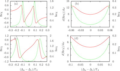
Figure 2: (Color online) $\chi$ and $d\chi/d\omega$ with different values of coupling fields strength and $\Delta$ when $R_{\rm op}=0$. Left figures show the $\chi$ versus two photon detuning, in which the red solid line and green dashed line represent the real and imaginary parts of $\chi$, respectively. The right figures show the real part of $d\chi/d\omega$ (red solid line) and the imaginary part of $\chi$ (green dashed line) between the two Raman peaks. (a),(b) $\Omega_{c}=20\Gamma_{3}$, $\Delta=0.1\Gamma_{3}$; (c),(d) $\Omega_{c}=30\Gamma_{3}$, $\Delta=0.2\Gamma_{3}$.

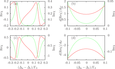
Figure 3: (Color online) $\chi$ and $d\chi/d\omega$ versus two photon detuning with different optical pump rates, when $\Omega_{c}=30\Gamma_{3}$ and $\Delta=0.2\Gamma_{3}$. The figures layout are the same as Fig. 2.(a),(b) $R_{\rm op}=0.06$; (c),(d) $R_{\rm op}=0.4\Gamma_{3}$.

When an optical pump from $\left|1\right>$ to $\left|2\right>$ is applied to the system, the Raman peaks change obviously. The $\chi$ and $d({\rm Re}\chi)/d\omega$ versus two photon detuning with the optical pump rates of 0.06$\Gamma_{3}$ and 0.4$\Gamma_{3}$ when $\Omega_{c}=30\Gamma_{3}$ and $\Delta=0.2\Gamma_{3}$ are shown in Fig. 3. Figures  3(a) and 3(b) show that when an optical pump is added to the system, the dispersion and absorption become much smaller compared with Figs. 2(c) and 2(d), while the shape of $\chi$ versus two photon detuning almost unchanged. Figures 3(c) and 3(d) show the result of a sufficient large optical pump added to the system. The two Raman absorptive peaks change into enhanced peaks, the normal dispersion changes into anomalous dispersion, while the FWHM of the Raman peaks and the ratio of the dispersion to the absorption(enhancement) of the system remain almost unchanged. The experimental demonstration of the control of the Raman peak using an optical pump has been done in our previous work PRA.73.053804 in room temperature paraffin coated rubidium 87 cell.

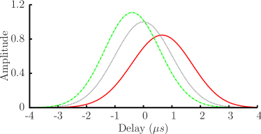
Figure 4: (Color online) Simulation of a 1 $\mu s$ Gaussian wave packet transmitting through 1 mm cold ⁸⁷Rb cloud with atomic density of $5\times 10^{11}/$cm³. The frequency difference of the coupling fields is 2$\Delta=0.4\Gamma_{3}$. The Rabi frequencies of the coupling fields are $\Omega_{c}=30\Gamma_{3}$. The red solid line is corresponding to the optical pump rate of $R_{\rm op}=0$, and $n_{g}=1.9\times 10^{5}$. The green dashed line is corresponding to the optical pump rate of $R_{\rm op}=0.4\Gamma_{3}$, and $n_{g}=-1.1\times 10^{5}$. The gray dot line is the reference.

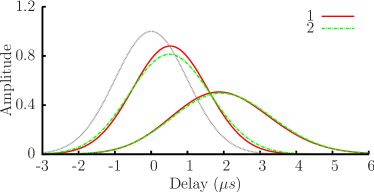
Figure 5: (Color online) Comparing the slow light effect with the EIT scheme. Line 1 is the slow light effect of EIT with different coupling strength, wave packets from right to left are corresponding to $\Omega_{c}=0.5\Gamma_{3}$ and $1\Gamma_{3}$, and $n_{g}=5.9\times 10^{5}$ and $1.6\times 10^{5}$. Line 2 is the slow light effect with different optical pump rate when $\Omega_{c}=55\Gamma_{3}$, wave packets from right to left are corresponding to $R_{\rm op}=0$, $0.17\Gamma_{3}$ and $n_{g}=6.0\times 10^{5}$ and $1.6\times 10^{5}$. The gray dot line is the reference.

To show the slow and fast light effect of this two-coupling scheme, we simulate a 1 $\mu s$ Gaussian probe field (FWHM$\>\approx 2.35\;\mu s$) transmitting through a 1-mm cold ⁸⁷Rb cloud with the atomic density of $5\times 10^{11}/$cm³. The $D1$ transitions used to create the $\Lambda$ system and the $D2$ transition for optical pump. The frequency difference of the two coupling is set to $0.4\Gamma_{3}$. In the simulation we suppose that the probe field is weak and almost do not influence the system. The slow light and fast light effects with the Rabi frequencies of the coupling fields of $30\Gamma_{3}$ are shown in Fig. 4. This figure shows clearly that when the optical pump is absent the probe field gets a positive group delay, while when certain optical pump is added, the probe field gets a negative group delay. This figure also shows that the probe field encounters little reshape, stretched by a factor of about 1.03 with the positive group delay, while narrowed by a factor of 0.95 with the negative group delay. In our simulation the probe pulse is a 1 $\mu s$ Gaussian wave packet, which corresponds to $\Delta\omega=1\times 10^{6}$ rad/$s$ and FWHM$\>\approx 2.35\times 10^{6}$ rad/$s$. While the FWHM of the transmission width of the system is about $6.6\times 10^{6}$ rad/$s$. The line width of the probe field is not far smaller than the transmission width, this causes the stretch and narrowing of the wave packet with positive and negative group delay. There are also some internal reasons which make the wave packet narrowed with the negative group delay. A system can not make a wave packet pass through before the arrival of this wave packet. The speed of the starting point of a wave packet should be slower than or equal to $c$. Therefore if the wave packet gets a negative group delay, it should be compressed in the time domain.

In order to examine the performance of this two-coupling scheme, a comparison between this two-coupling scheme and the normal EIT scheme in the slow light region is given. The EIT scheme is the best slow light scheme in the atomic system to our best knowledge. The system parameters used are the same as the above simulation. The results are shown in Fig. 5. We compare the two schemes with almost the same delay occurred. In Fig. 5, line 1 shows the results of the EIT scheme with different coupling strengths and line 2 shows the results of the two-coupling scheme with different pump rates. The figure shows that when the optical pump is absent the two-coupling scheme almost has the same effect with the EIT scheme, the same delay causes the same stretch, as shown in the right wave packets of Fig. 5. This demonstrates that in the slow light region this two-coupling scheme is comparable with the EIT scheme. In the EIT scheme the coupling power is increased to make the probe pulse get less delay, and as the increment of the coupling power the transmission width for the probe field will get larger, while if we use the optical pump in the two-coupling scheme to make the probe field get less delay, the transmission width do not change. Therefore in this case the wave packet delayed by the two-coupling scheme will get a larger stretch than the EIT scheme, as shown in the left wave packets of Fig. 5.

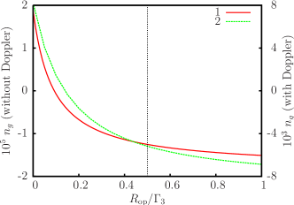
Figure 6: (Color online) The relation between $n_{g}$ and the optical pump rate when $\Omega_{c}=30\Gamma_{3}$, $\Delta=0.2\Gamma_{3}$, using the same system parameters as Fig. 4. Line 1: without Doppler broadening, line 2: with Doppler broadening. The Doppler broadening is calculated using the data of ⁸⁷Rb at 320 K.

We also calculate the change of $n_{g}$ versus $R_{\rm op}$ with the same system parameters in ⁸⁷Rb as the simulation above. The results are shown in Fig. 6. The figure shows clearly that as the increment of $R_{\rm op}$ the $n_{g}$ get more and more smaller and then become negative. The system will get saturated as the increment of the optical pump rate, which set the limitation of the largest negative group velocity when $\Omega_{c}$ and $\Delta$ are fixed. The vertical line in Fig. 6 gives the upper bound of the optical pump rate derived from Eq. (4) (using $\Gamma_{52}=\Gamma_{3}/2$), which means the largest optical pump rate can be got when level $|5\rangle$ is a single energy level. When multiple excited states are used for optical pump or $\Gamma_{52}>\Gamma_{3}/2$, this bound might be exceeded. Fig. 6 also shows that the Doppler broadening affects only the scale of $n_{g}$ and the optical pump strength needed to change the dispersion from normal to anomalous.

At last we would like to point out that this scheme can be simplified. In a normal three-level system the Raman peaks can also be flipped by the optical pump, although the two Raman peaks will not be symmetric. Furthermore, the normal and anomalous dispersions can also be observed at the root of the Raman peak when only one coupling is used.

In summary, we have shown a scheme based on the far detuning Raman effect to control the light speed from slower-than-$c$ to faster-than-$c$. The dispersion of the system can be controlled by an optical pump, so the velocity of the probe beam can be changed dynamically by controlling the strength of the optical pump. Theoretically, this scheme can provide an arbitrary large positive or negative dispersion, however the largest dispersion is limited by the bandwidth of the system, which are decided by the parameters of the system used, e.g. optical depth of the atomic system, strength of the couplings. Our scheme is very easy in realization, since the requirements are quite simple: a system, which can generate Raman peaks in far detuning $\Lambda$ structure and an additional level used for optical pump, can be used to realize this scheme. Almost any system in which EIT can be observed is suitable to realize this scheme. Although a four-level system, whose electronic dipole moments fulfill the requirement mentioned in the second paragraph, will be better, a normal three level structure can be used too. There is no any technical difficulty too, since the key point of this scheme is the far detuning Raman peaks which can be flipped using an optical pump. Fortunately, this has already been demonstrated in experimentPRA.73.053804 .

- (1) A. Kasapi, M. Jain, G. Y. Yin, and S. E. Harris, Phys. Rev. Lett. 74, 2447 (1995).
- (2) O. Schmidt, R. Wynands, Z. Hussein, and D. Meschede, Phys. Rev. A 53, R27 (1996).
- (3) L. V. Hau, S. E. Harris, Z. Dutton, and C. H. Behroozi, Nature 397, 594 (1999).
- (4) M. M. Kash et al., Phys. Rev. Lett. 82, 5229 (1999).
- (5) D. Budker, D. F. Kimball, S. M. Rochester, and V. V. Yashchuk, Phys. Rev. Lett. 83, 1767 (1999).
- (6) A. V. Turukhin et al., Phys. Rev. Lett. 88, 023602 (2001).
- (7) M. S. Bigelow, N. N. Lepeshkin, and R. W. Boyd, Phys. Rev. Lett. 90, 113903 (2003).
- (8) S. E. Harris, J. E. Field, and A. Imamoglu, Phys. Rev. Lett. 64, 1107 (1990).
- (9) M. Fleischhauer, A. Imamoglu and J. P. Marangos, Rev. Mod. Phys. 77, 633 (2005).
- (10) L. J. Wang, A. Kuzmich, and A. Dogariu, Nature 406, 277 (2000).
- (11) M. S. Bigelow, N. N. Lepeshkin, and R. W. Boyd, Science 301, 200 (2003).
- (12) M. S. Bigelow, N. N. Lepeshkin, and R. W. Boyd, J. Phys. Cond. Mat. 16, R1321 (2004).
- (13) S. Longhi, Phys. Rev. E 72, 056614 (2005).
- (14) I. Guedes, L. Misoguti, and S. C. Zilio, Opt. Express 14, 6201 (2006).
- (15) C. Goren, A. D. Wilson-Gordon, M. Rosenbluh, and H. Friedmann, Phys. Rev. A 68, 043818 (2003).
- (16) D. Bortman-Arbiv, A. D. Wilson-Gordon, and H. Friedmann, Phys. Rev. A 63, 043818 (2001).
- (17) G. S. Agarwal, T. N. Dey, and S. Menon, Phys. Rev. A 64, 053809 (2001).
- (18) D. A. Steck, Alkali d line data, http://steck.us/alkalidata/, (2003).
- (19) W. Jiang, Q.-F. Chen, Y.-S. Zhang, and G.-C. Guo, Phys. Rev. A 73, 053804 (2006).