Diversity Multiplexing Tradeoff of Asynchronous Cooperative Relay Networks

Abstract

The assumption of nodes in a cooperative communication relay network operating in synchronous fashion is often unrealistic. In the present paper we consider two different models of asynchronous operation in cooperative-diversity networks experiencing slow fading and examine the corresponding diversity-multiplexing tradeoffs (DMT). For both models, we propose protocols and distributed space-time codes that asymptotically achieve the transmit diversity bound for all multiplexing gains and for any number of relays.

1 Introduction

In fading relay channels cooperative diversity has been introduced as a technique to provide spatial diversity to help combat fading. Cooperation creates a virtual transmit antenna array between the source and the destination that provides the needed spatial diversity. Cooperative diversity protocols can be broadly classified as belonging to either the class of Amplify and Forward (AF) or Decode and Forward (DF) protocols, depending on the mode of operation of the intermediate relays. In order to fully reap the benefits of user cooperative diversity, it is necessary for the network to operate synchronously. However, in practical distributed wireless systems, this may be difficult to achieve. As a result, cooperative-diversity schemes that are designed assuming perfect timing synchronization, may not be able to fully exploit the benefits of cooperation in the absence of synchronization. This motivates the study of cooperation schemes that are robust to network timing errors.

Figure 1: Cooperative Relaying in networks.

1.1 Setting and Channel Model

We consider two-hop networks with $N$ relays. We will use the diversity multiplexing tradeoff (DMT) proposed by Zheng and Tse [5] as a performance measure. We analyze two-hop networks with and without a direct link between source and sink. When there is a direct link, we will assume that the relays are isolated. This is to make the DMT analysis tractable. In the synchronous case, and in the presence of relay isolation, there exist protocols that are known to achieve the optimal DMT of the network, whereas in the absence of relay isolation, the optimal DMT of the two-hop network with direct link remains an open problem. For networks with no direct link we relax this assumption and are able to handle scenarios in which there is interference between the relays.

We follow the literature in making the assumptions listed below concerning the channel. Our descriptions are in terms of the equivalent complex-baseband, discrete-time channel.

1. All nodes have a single transmit and single receive antenna.

2. The nodes operate in a half-duplex fashion; i.e., at any instant a node can either transmit or receive but not do both.

3. All channels are assumed to be quasi-static and to experience Rayleigh fading and hence all fade coefficients are assumed to be i.i.d., circularly-symmetric, complex gaussian $\mathbb{C}\mathcal{N}(0,1)$ random variables.

4. The additive noise at each receiver is also modeled as possessing an i.i.d., circularly-symmetric, complex gaussian, $\mathbb{C}\mathcal{N}(0,1)$ distribution.

5. The destination (but none of the relays) is assumed to have perfect knowledge of all the channel gains.

We denote the $i^{th}$ relay by $R_{i}$. The channel gain from the source to the relay $R_{i}$ will be denoted by $g_{i}$, the gain from the relay $R_{i}$ to the destination by $h_{i}$ and between the relays $R_{i}$ and $R_{j}$ relays by ${\gamma}_{ij}$. The gain for the direct link, if present, will be denoted by $g_{0}$. All protocols considered in this work are slotted protocols. This means that the nodes operate according to a schedule which determines the time slots in which a node should listen and the time slots in which it should transmit. In its designated time slot, a node either receives or transmits a vector of length $T$ channel uses which will be referred to as a packet.

1.2 Prior Work

The concept of user cooperative diversity was introduced in [1, 2]. Cooperative diversity protocols were first discussed in [3] for the two-hop single-relay network. Zheng and Tse [5] proposed the Diversity-Multiplexing gain Tradeoff (DMT) as a tool to evaluate point-to-point multiple-antenna schemes in the context of slow fading channels. The DMT was subsequently used as a tool to compare various protocols for half-duplex, two-hop cooperative networks in [4, 6], see also [9]-[13]. Reference [10] addresses the DMT of the more general class of multi-hop cooperative relay networks. Jing and Hassibi ([15]) consider a two hop network without the direct link, analyze the probability of error and propose code design criteria in order to achieve full cooperative diversity. All the above works assume that all relay nodes are perfectly synchronized.

We summarize below results in the recent literature that address timing errors in cooperative networks.

In [16] and [18], the authors analyze two-hop networks without a direct link and construct distributed space-time trellis codes that achieve full cooperative diversity under asynchronism. They consider decode-and-forward two-phase protocols. Relative propagation delays between source and the relays as well as from the relays to the destination are assumed to be the source of timing error. It is assumed that the destination transmits a beacon to signify reception of a codeword matrix. In [17], an Alamouti-based strategy that facilitates single-symbol decodability is proposed for asynchronous relay networks, that achieves a diversity order of two for any number of relays. Codes with low decoding complexity achieving full diversity for any number of relays, in the presence of asynchronism were constructed in [19].

Damen and Hammons ([20]) construct delay-tolerant distributed TAST block codes that achieve full diversity for the two-phase protocol in the presence of delays, under the decode and forward (DF) strategy. Their constructions are flexible in terms of accommodating a varying number of transmit and receive antennas as well as varying decoding complexity.

Wei considers the two-hop network with delays in [21] and analyzes the DMT of certain protocols. For the two phase DF protocol, [21] considers both the scenario where the relay performs independent coding as well as one in which joint distributed space time coding is carried out and the author then goes on to evaluate the DMT of the two schemes. However, these schemes do not meet the cut-set bound on DMT for all values of multiplexing gain.

1.3 Results

We consider two different models of asynchronous operation in cooperative relay networks:

1. the propagation-delay model

2. the slot-offset model.

For both these models we propose a variant of the Slotted Amplify and Forward (SAF) protocol proposed in [9] which asymptotically achieves the transmit diversity bound in the absence of a direct source-destination link, for any number of relays and for an arbitrary delay profile. When there is a direct link we achieve the transmit diversity bound under the assumption that all the relays are isolated. We also present DMT optimal codes for both cases considered above.

2 Slotted Amplify and Forward Protocol for the Propagation-Delay Model

2.1 Propagation Delay Model

Under this model we take into account the relative propagation delays between the various nodes. We assume that the delay is in units of one symbol duration (i.e., one channel use). We adopt the following notation: the pair $(\nu_{i},\pi_{i})$ denotes the delay between source and relay $R_{i}$ and between relay $R_{i}$ and the destination respectively. The overall delay in the $i^{th}$ relay path will be denoted by $\tau_{i}$. Thus $\tau_{i}=\nu_{i}+\pi_{i}$. Set

$$\theta\ =\ \max_{1\leq i\leq N}{\tau_{i}}.$$

We will make the simplifying assumption that the delay between any two relays is zero. It turns out that the lower bounds on DMT that we derive here, will only improve in the presence of inter-relay delays. All delays are assumed to be known at the destination. The relays are assumed to know the propagation delay from source to the respective relay to the extent that that the relay node knows when it is receiving its intended packet from the source.

Synchronous network operation implies in particular, packet-level synchronization. As a result, packets arriving at either a relay node or the destination, originating at either the source or a relay node, are aligned in time and thus it is meaningful to speak of interfering packets. This will no longer be the case if there exists relative propagation delays as there will now be relative time-shifts between packets arriving from various nodes, either at a relay node or at the destination.

2.2 DMT Analysis of the Quasi-Synchronous Network under the Naive SAF Protocol

We consider a particular AF protocol, known in the literature as the Slotted Amplify and Forward (SAF) protocol, and proposed by Yang and Belfiore [9]. We give a brief description of the protocol here as applied to the case when there is no direct link from source to destination. An $N$-relay $M$-slot SAF operates as follows:

1. The protocol splits up the time axis into frames and slots. There are $T$ channel uses per slot and $(M+1)$ slots per frame, where $M=KN$ is a multiple of the number $N$ of relays. The slots are indexed from $0$ through $M$. If one ignores the first initialization slot (slot zero), then there are in effect $M$ slots per frame. Under the SAF protocol, the $M$ slots are divided into $K$ cycles, each cycle being of time duration equal to $NT$ channel uses (see Fig. 2).

2. In the first, initialization slot, the source transmits $\underline{x}_{0}$ and during the $i^{th}$ slot $1\leq i\leq M-1$, the vector $\underline{x}_{i}\ =\ [x_{iT+1}\ x_{iT+2}\ \ldots\ x_{(i+1)T}]$ is transmitted.

3. During the $i$th time slot, $1\leq i\leq M$, the $j$th relay, $R_{j}$, where $j$, $1\leq j\leq N$, is such that $j\ =\ i\pmod{N}$, forwards the $\underline{s}_{i}$ signal received by it during the immediately preceding, i.e., $(i-1)$th slot. However, to simplify the description, we will write $R_{i}$ in place of $R_{j}$. Thus for example, if $N=4$, during the $7$th time slot, we will speak of relay $R_{7}$ as forwarding the signal received by it during the $6$th time slot, when we actually mean relay $R_{3}$, since $7=3\pmod{4}$. Note that $\underline{s}_{i}$ includes the additive noise present in the receiver of the $i$th relay. One round of transmissions by all the relays constitutes a cycle. Thus each frame is comprised of $K$ cycles with each relay transmitting precisely once during each cycle. The source remains silent in the final, $M^{th}$ slot (see Fig. 3).

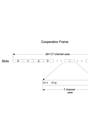
Figure 2: Cooperation frame for SAF.

We now write down an expression for the signals received by relay and destination during the $i^{th}$ slot. The relay $R_{i+1}$ receives

$$\underline{s}_{i} = g_{i+1}\underline{x}_{i}+\gamma_{i,i+1}\underline{s}_{i-1}+\underline{v}_{i}$$ (1)

where $\underline{s}_{i-1}$ is the signal transmitted by $R_{i}$. The signal received at the destination is given by

$$\underline{y}_{i}=h_{i}\underline{s}_{i-1}+\underline{w}_{i}.$$ (2)

Here $\underline{v}_{i}$ and $\underline{w}_{i}$ denote white noise. Fig. 3 depicts the protocol operation for $N=3$ and $M=6$.

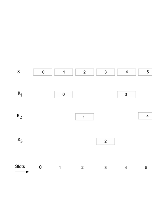
Figure 3: SAF protocol for the case of $N=3$ relays, and a total of $M+1=7$ slots.

The destination collects the vector of received symbols and at the end of one frame the resulting channel model can be written as,

$$\underline{y}=H\underline{x}+G\underline{v}+\underline{w}.$$

Here $\underline{x}=\left[\underline{x}_{0}\ \underline{x}_{1}\ \ldots\ \underline{x}_{M-1}\right]$ is the vector of transmitted symbols and $H$ is a lower triangular matrix of size $MT\times MT$. The main diagonal of $H$ consists of entries of the form $\gamma_{i}=h_{i}g_{i}$, each entry being repeated $K$ times. $G$ is a matrix consisting of channel gains. The resulting noise term $G\underline{v}+\underline{w}$ is not white in general. But it has been shown in [10] that for the class of AF protocols in general the resulting noise at the destination is white in the scale of interest. Hence from now on we will work with the model

$$\underline{y}=H\underline{x}+\underline{w}$$

with $\underline{w}$ being white. The DMT of the above matrix can be lower bounded by

$$d(r)\geq N\left(1-\frac{M+1}{M}r\right)$$

which meets the transmit diversity bound as $M$ tends to infinity. For the case with direct link, the protocol remains the same as above except that the source transmits in the $M^{th}$ slot as well. This is shown to asymptotically achieve the DMT $(N+1)(1-r)$ under the assumption that all the relays are isolated; i.e., a relay cannot hear what the other relays transmit( see [9]). However the exact DMT of the SAF protocol without the assumption of relay isolation remains an open problem. A lower bound to the DMT of the SAF protocol under the assumption of relay-isolation can also be found derived in [10].

2.2.1 Impact of Propagation Delays on the DMT

We now analyze the impact of delays on the operation of the naive SAF protocol for the case of a two-hop network without direct link. Throughout this sub-section, we will assume quasi-synchronous operation of the network, by which we will mean that there is no propagation delay between the source and any of the relay nodes. Thus the value $\nu_{i},i=1,2,\ldots,N$ of these delays from the source to the relays are all set equal to zero. In order to isolate different frames, the source extends the silence in the last slot to $T+\theta$ channel uses in place of $T$ channel uses in naive SAF. The analysis of this simple network will serve to illustrate the performance degradation of naive SAF and will also provide insights on how to handle the general case when both $\nu_{i}$ and $\pi_{i}$ are non zero. We now introduce some terminology. When the symbols in a packet are arranged chronologically, those appearing at the beginning will be called the head of the packet while the tail of the packet will correspond to symbols at the end.

Since each $\nu_{i}=0$, the signals received at the relays are exactly the same as that in the case of perfect synchronization (see Fig. 4(a)). As per the SAF protocol, while the relay $R_{i+1}$ is listening to packet $\underline{x}_{i}$ from the source in the $i^{th}$ slot, the relay $R_{i}$ will be transmitting packet $\underline{s}_{i-1}$. Thus relay $R_{i+1}$ will simultaneously receive transmissions from the source and relay node $R_{i}$ and these transmissions will moreover, be aligned in time. This however, is not the situation at the destination. Depending upon the value of the relative delays $\pi_{i}$, the tail of the transmission from relay node $R_{i}$ could for instance, interfere with the head of the transmission from relay node $R_{i+1}$. This is depicted in Fig. 4(b).

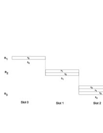
(a) Reception at the relays

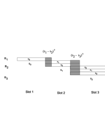
(b) Reception at the destination

Figure 4: Reception at the relays and destination

The receptions at the destination will get modified as,

$$\underline{y}_{i} = h_{i}\underline{s}_{i-1}+h_{i-1}D^{T-\Delta\tau_{i-1}}(\underline{s}_{i-2})+h_{i+1}D^{T-\Delta\tau_{i}}(\underline{s}_{i})+\underline{w}_{i}.$$ (3)

Notice that in addition to the intended reception from relay $R_{i}$ there is interference from relays $R_{i-1}$ and $R_{i+1}$. Here $D^{T-\Delta\tau_{i}}$ corresponds to a shift-and-truncate operator acting on a vector of symbols. The direction of shift depends upon the sign of $\Delta\tau_{i}=(\tau_{i}-\tau_{i+1})$. If $\Delta\tau_{i}$ is positive (negative) then $D^{T-\Delta\tau_{i}}\underline{x}$ shifts $\underline{x}$ to the right (left) by $(T-|\Delta\tau_{i}|)$ symbols and drops the last (first) $(T-\Delta\tau_{i})$ symbols.

The signal received by the destination over the course of one frame can be expressed in the form

$$\underline{y}=H\underline{x}+\underline{w}.$$

Here, unlike in the synchronous case, the resulting channel matrix $H$ will no longer be lower-triangular. We illustrate with an example where $N=3,M=3,T=3$. In the case of perfect synchronization, the channel matrix at the destination would look like,

$$\left[\begin{array}[]{c}y_{0}\\ y_{1}\\ y_{2}\\ y_{3}\\ y_{4}\\ y_{5}\\ y_{6}\\ y_{7}\\ y_{8}\\ \end{array}\right] = \left[\begin{array}[]{ccccccccc}\gamma_{1}\\ &\gamma_{1}\\ &&\gamma_{1}\\ \beta_{1}&&&\gamma_{2}\\ &\beta_{1}&&&\gamma_{2}\\ &&\beta_{1}&&&\gamma_{2}\\ \beta_{3}&&&\beta_{2}&&&\gamma_{3}\\ &\beta_{3}&&&\beta_{2}&&&\gamma_{3}\\ &&\beta_{3}&&&\beta_{2}&&&\gamma_{3}\\ \end{array}\right]\left[\begin{array}[]{c}x_{0}\\ x_{1}\\ x_{2}\\ x_{3}\\ x_{4}\\ x_{5}\\ x_{6}\\ x_{7}\\ x_{8}\\ \end{array}\right]+\underline{w}$$ (31)

where $\beta_{1}=g_{1}h_{2}\gamma_{12}$, $\beta_{2}=g_{2}h_{3}\gamma_{23}$, $\beta_{3}=g_{1}h_{3}\gamma_{12}\gamma_{23}$. However, in the presence of delays $\pi_{1}=2,\ \pi_{2}=1$ and $\pi_{3}=0$, the resulting channel matrix takes on the form

$$\left[\begin{array}[]{c}y_{0}\\ y_{1}\\ y_{2}\\ y_{3}\\ y_{4}\\ y_{5}\\ y_{6}\\ \end{array}\right] = \left[\begin{array}[]{ccccccccc}\gamma_{1}\\ &\gamma_{1}\\ \beta_{1}&&\gamma_{1}&\gamma_{2}\\ &\beta_{1}&&&\gamma_{2}\\ \beta_{3}&&\beta_{1}&\beta_{2}&&\gamma_{2}&\gamma_{3}\\ &\beta_{3}&&&\beta_{2}&&&\gamma_{3}\\ &&\beta_{3}&&&\beta_{2}&&&\gamma_{3}\\ \end{array}\right]\left[\begin{array}[]{c}x_{0}\\ x_{1}\\ x_{2}\\ x_{3}\\ x_{4}\\ x_{5}\\ x_{6}\\ x_{7}\\ x_{8}\\ \end{array}\right]+\underline{w}.$$ (55)

It is not easy, in general, to compute the DMT of channel matrices $H$ having structure of the form appearing above. The difficulty arises precisely from terms like $\gamma_{i}x_{i}+\gamma_{i+1}x_{i}$ that are heard at the destination due to simultaneous reception from two relays. One possible way to lower bound the DMT is to drop some symbols from the received vector such that the channel matrix between the remaining subset of input and output symbols is lower triangular. For if the matrix is lower triangular, we can use results from [10] to lower bound the DMT. For the channel in equation 55, it is clear that after dropping $\{y_{2},y_{4},y_{6}\}$ the resulting channel model will be

$$\left[\begin{array}[]{c}y_{0}\\ y_{1}\\ y_{3}\\ y_{5}\\ \end{array}\right] = \left[\begin{array}[]{cccc}\gamma_{1}\\ &\gamma_{1}\\ &\beta_{1}&\gamma_{2}\\ &\beta_{3}&\beta_{2}&\gamma_{3}\\ \end{array}\right]\left[\begin{array}[]{c}x_{0}\\ x_{1}\\ x_{4}\\ x_{7}\\ \end{array}\right].$$ (68)

We now show through a sequence of mutual information inequalities that the DMT of the resulting channel, after dropping certain terms, is indeed a lower bound for the DMT of the original matrix. Let $\underline{x}_{A}$ and $\underline{y}_{B}$ be the vector of input and output symbols that we retain. Then

$$I(\underline{x};\underline{y}|H) = I(\underline{x}_{A},\underline{x}_{A^{c}};\underline{y}_{B},\underline{y}_{B^{c}}|H)$$ (69)

$$\geq I(\underline{x}_{A},\underline{x}_{A^{c}};\underline{y}_{B}|H)$$

$$= I(\underline{x}_{A};\underline{y}_{B}|H)+I(\underline{x}_{A^{c}};\underline{y}_{B}|\underline{x}_{A},H)$$

$$\geq I(\underline{x}_{A};\underline{y}_{B}|H)=I(\underline{x}_{A};\underline{y}_{B}|H^{\prime})$$

where $H^{\prime}$ is the channel relating $\underline{x}_{A}$ and $\underline{y}_{B}$, i.e.,

$$\underline{y}_{B}=H^{\prime}\underline{x}_{A}+\underline{w}^{\prime}.$$

We now provide a systematic way in which we can drop symbols at the destination so that the resulting channel matrix is lower triangular. This is by identifying and removing unintended interference at the destination. We call the interference between the tail of a packet and the head of the next immediate packet at the destination as collision. It is clear that since collision is an event that does not happen in the synchronous case, we have to drop the symbols involved in collision in order to retain the channel structure. Now, say packet $\underline{s}_{i-2}$ collided with $\underline{s}_{i-1}$ but $\underline{s}_{i-1}$ did not collide with $\underline{s}_{i}$. From equation (1) it is clear that the symbols in $\underline{s}_{i-1}$ that were involved in collision would be present in the form of interference in $\underline{s}_{i}$. This interference is also unintended and hence these symbols have to be dropped when $\underline{s}_{i}$ reaches the destination. We call such interference as corruption. It is different from collision since it happens at the relays. For if the relays were isolated there would be no corruption at all. It must be noted that collision is the cause of corruption. In a network where all the source to destination delays are equal but arbitrarily split between the source to relay and the relay to destination paths, the DMT of the SAF protocol remains unchanged.

Let us bound the number of symbols that need to be dropped from every packet due to collisions and corruptions. We may drop symbols from packet $\underline{y}_{i}$ as a consequence of one or more of the following events:

1. Collision at head with $\underline{s}_{i-2}$.

2. Collision at tail with $\underline{s}_{i}$.

3. Corruption at tail due to $\underline{s}_{i-2}$.

The number of symbols involved in the collision at head is $(\pi_{i-1}-\pi_{i})^{+}$ and similarly at tail it is $(\pi_{i}-\pi_{i+1})^{+}$. The number of corrupted symbols in the tail of $\underline{s}_{i-1}$ is again at most $(\pi_{j}-\pi_{j+1})^{+}$ for some $j$. Hence the number of symbols that need to be dropped can be bounded by $2\max_{j}(\pi_{j}-\pi_{j+1})^{+}$. Since we are interested in designing protocols for a certain maximum delay $\theta$ we further bound this as $2\theta$. Thus if we drop $T-2\theta$ symbols from each slot of the received vector, the resulting channel matrix will be lower triangular, the DMT of which can be bounded easily.

2.2.2 Lower Bound on DMT

At the end of a frame, after dropping some symbols, the destination would have received a vector of length $M(T-2\theta)$. The channel model can be written as,

$$\underline{y} = H\underline{x}+\underline{w}$$ (70)

where

$${\underline{x}}^{t} = \left[\begin{array}[]{ccccc}\underline{x_{0}}^{t}&\underline{x_{1}}^{t}&\underline{x_{2}}^{t}&\cdots&\underline{x_{M-1}}^{t}\end{array}\right]$$ (72)

is the vector of clean symbols, $H$ is the $M(T-2\theta)\times M(T-2\theta)$ channel matrix and $\underline{w}\ \epsilon\ \mathcal{C}^{M(T-2\theta)}$ is the noise vector. The channel matrix $H$ is lower triangular. The structure of the lower triangular half of the matrix depends on the delay profile of the network. We have the following result.

Proposition 1

For the protocol described in section 2.2 the DMT is lower bounded by

$$d(r)\geq N\left(1-\frac{(M+1)T+\theta}{M(T-2\theta)}r\right)$$

which asymptotically approaches the transmit diversity bound for large $M$ and $T$.

In order to derive a lower bound on the DMT of the proposed protocol we make use of the following important result from [10].

Theorem 2

([10]) Let $H$ be a lower triangular matrix with random entries. Let $H_{d}$ be a diagonal matrix whose diagonal entries are the same as the main diagonal entries of $H$, and let $H_{l}$ be a matrix consisting of only the last sub diagonal of $H$ and zeros else where. Let $d_{H}(r),d_{H_{d}}(r)$ and $d_{H_{l}}(r)$ denote the DMT of these matrices respectively. Then

1. $d_{H}(r)\geq d_{H_{d}}(r)$.

2. $d_{H}(r)\geq d_{H_{l}}(r)$.

3. In addition, if the entries of $H_{d}$ and $H_{l}$ are independent, then $d_{H}(r)\geq d_{H_{d}}(r)+d_{H_{l}}(r)$.

Proof of proposition 1: Consider the channel model given by (70). Let $T^{{}^{\prime}}=T-2\theta$. Let $H_{d}$ be the corresponding diagonal matrix associated with $H$. The diagonal entries of $H_{d}$ are the product fade coefficients $h_{i}g_{i}$ each repeated $KT^{{}^{\prime}}$ times. Let us denote $\gamma_{i}=h_{i}g_{i}$. The entries below the principal diagonal are products of $h_{i}$’s and $g_{i}$’s which are correlated with $\gamma_{i}$’s. Hence we make use of implication 1 of theorem 2. Let $r^{{}^{\prime}}=((M+1)T+\theta)r$. The DMT of the diagonal matrix $H_{d}$ can be easily calculated as follows:

$$Pr\{I(\underline{x};\underline{y}|H_{d})\leq r^{{}^{\prime}}\log\rho\} = Pr\{\log\det(I+\rho H_{d}H_{d}^{\dagger})\leq r^{{}^{\prime}}\log\rho\}$$ (73)

$$= Pr\{\log(\prod_{i=1}^{N}(1+\rho|\gamma_{i}|^{2})^{KT^{{}^{\prime}}})\leq r^{{}^{\prime}}\log\rho\}$$ (74)

$$= Pr\{KT^{{}^{\prime}}\sum_{i=1}^{N}(1-\alpha_{i})^{+}\leq r^{{}^{\prime}}\}$$ (75)

where $|\gamma_{i}|^{2}=\rho^{-\alpha_{i}},i=1,2,\ldots,N$. Therefore we have,

$$d_{H_{d}}(r) = \inf_{KT^{{}^{\prime}}\sum_{i=1}^{N}(1-\alpha_{i})^{+}\leq r^{{}^{\prime}}}(\sum_{i=1}^{N}\alpha_{i})$$ (76)

$$= N\left(1-\frac{(M+1)T+\theta}{M(T-2\theta)}r\right).$$ (77)

By theorem 2, a lower bound on the DMT of the proposed protocol can be given by

$$d_{H}(r)\geq d_{H_{d}}(r)=N\left(1-\frac{(M+1)T+\theta}{M(T-2\theta)}r\right)$$

which asymptotically approaches the transmit diversity bound for large $M$ and $T$. As M tends to infinity we have

$$d_{H}(r)\geq N\left(1-\frac{T}{T-2\theta}r\right).$$ (78)

 

From equation (78), we see that there is a rate loss factor of $\frac{T}{T-2\theta}$. This factor reflects the loss in maximum multiplexing gain for a finite slot length but arbitrarily large number of cycles. This is actually the ratio of the length of one slot to the number of clean symbols per slot for the protocol. In the next sub-section we show how padding zeros at the source helps in increasing the number of clean symbols per slot, thereby increasing the resulting DMT.

2.3 SAF Protocol with Guard Time for the Network with Arbitrary Delay Profile

From the analysis in section 2.2.1, it is clear that a simple way to ensure lower-triangular structure of the channel matrix is to include a guard time for each slot, thereby avoiding collisions at the destination. By guard time we mean a period of silence where the source transmits nothing, thereby slowing down its operation. The guard time ensures that the number of colliding symbols at the destination is reduced.

Let $x$ be the length of the guard time per slot. Now the effective length of every slot is $T^{{}^{\prime}}=T+x$. The strategy adopted by the relays is as follows: Every relay listens to the source for $T$ channel uses and transmits in the next $T$ immediate channel uses. As described in the previous sub-section the destination collects only the collision free symbols in every slot. Then it is easy to see that the number of clean symbols in every slot can be lower bounded by $(T-2\theta+2x)$. Thus adding $x$ guard symbols provides a two-fold increase in the number of clean symbols. Following similar outage analysis as in section 2.2.1, the DMT of the resulting SAF protocol with guard time can be lower bounded as,

$$d(r) \geq N\left(1-\frac{T+x}{T-2\theta+2x}r\right).$$ (79)

In particular when $x=\theta$ we have

$$d(r) \geq N\left(1-\frac{T+\theta}{T}r\right).$$ (80)

The lower bound in equation (80) is better than that in equation (79) for $x\leq\theta$. Thus padding $\theta$ zeros in every slot gives the optimal guard time and it completely eliminates collision. Padding more than $\theta$ zeros only reduces the DMT as the number of clean symbols in every slot can at most be only $T$.

Even for the more general case where there are delays from the source to the relays as well, it can be shown through a similar analysis as in section 2.2 that the number of clean symbols per slot for naive SAF can be bounded as ($T-2(\tau_{\max}-\tau_{\min})$) in place of ($T-2\max\{(\tau_{i}-\tau_{i+1})\}$) for the quasi synchronous network. A guard time of $\theta$ would be sufficient in this case, the details of which are provided in the next section.

2.3.1 Case with no Direct Link

We first consider the two-hop network without the direct link. We show that the SAF protocol with guard time asymptotically achieves the transmit diversity bound for any delay profile (${\nu}_{i},{\pi}_{i}$), $i=1,2,\ldots,N$. The description of the protocol is as follows:

1. There are totally $(M+1)$ slots in a frame. The source operation is the same as that in naive SAF described in section 2, except that in each of the first $M$ slots the source flushes $\theta$ zeros after sending $T$ information symbols. The total duration of one frame is $(M(T+\theta)+T)$ channel uses.

2. Each relay in its respective slot, listens for $T$ channel uses and transmits in the next immediate $T$ channel uses.

The signal received by the relay $R_{i+1}$ in the $i^{th}$ slot is given by,

$$\underline{s}_{i} = g_{i+1}\underline{x}_{i}+D^{\Delta\nu_{i}}\ \gamma_{i,i+1}\underline{s}_{i-1}+\underline{v}_{i}$$ (81)

where $\underline{s}_{i-1}$ is the signal transmitted by relay $R_{i}$. Here $D^{\Delta\nu_{i}}$ is again a shift-and-truncate operator which operates as follows. If $\Delta_{i}$ is positive (negative) then $D^{\Delta\nu_{i}}$ shifts $\underline{x}$ to the right (left) by $|\Delta\nu_{i}|$ symbols and drops the last (first) $|\Delta\nu_{i}|$ symbols.

The signal transmitted by the relay $R_{i}$ arrives at the destination with a delay of $\pi_{i}$. By padding $\theta$ zeros we ensure that the receptions at destination from different relay nodes are made orthogonal. It is clear that these receptions will remain orthogonal even if there are inter-relay delays. Hence adding a guard time Notice that the different relay transmissions will also now be orthogonal. There is a total delay of $\tau_{i}$ in the $i^{th}$ path from the source to the destination. As the destination is assumed to know all the delays in the network it knows exactly when the transmission and the reception of a particular relay starts and ends and hence listens to the network only during these time instants. At the end of one frame the destination would have received a vector of length $MT$ consisting of the receptions from all the relays. The channel model is given by,

$$\underline{y} = H\underline{x}+\underline{w}$$ (82)

where

$$\underline{x}^{t} = \left[\begin{array}[]{ccccc}\underline{x}_{0}^{t}&\underline{x}_{1}^{t}&\underline{x}_{2}^{t}&\cdots&\underline{x}_{M-1}^{t}\end{array}\right]$$ (84)

is the vector of transmitted symbols from the source, $H$ is the $MT\times MT$ channel matrix and $\underline{w}\ \epsilon\ \mathcal{C}^{MT}$ is the noise vector. The channel matrix $H$ is lower triangular, which is a result of padding $\theta$ zeros to every slot. We then have the following theorem.

Theorem 3

For the protocol described in section 2.3.1 the DMT is lower bounded by

$$d(r)\geq N\left(1-\frac{M(T+\theta)+T}{MT}r\right)$$

which asymptotically approaches the transmit diversity bound for large $M$ and $T$.

Proof: Consider the channel model given by (82). Let $H_{d}$ be the corresponding diagonal matrix associated with $H$. The diagonal entries of $H_{d}$ are the product fade coefficients $h_{i}g_{i}$ each repeated $KT$ times, where $K=\frac{M}{N}$. Let us denote $\gamma_{i}=h_{i}g_{i}$. Let $r^{{}^{\prime}}=(M(T+\theta)+T)r$. The DMT of the diagonal matrix $H_{d}$ can be easily calculated as follows:

$$Pr\{I(\underline{x};\underline{y}|H_{d})\leq r^{{}^{\prime}}\log\rho\} = Pr\{\log\det(I+\rho H_{d}H_{d}^{\dagger})\leq r^{{}^{\prime}}\log\rho\}$$ (85)

$$= Pr\{\log(\prod_{i=1}^{N}(1+\rho|\gamma_{i}|^{2})^{KT})\leq r^{{}^{\prime}}\log\rho\}$$ (86)

$$= Pr\{KT\sum_{i=1}^{N}(1-\alpha_{i})^{+}\leq r^{{}^{\prime}}\}$$ (87)

where $|\gamma_{i}|^{2}=\rho^{-\alpha_{i}},i=1,2,\ldots,N$. Therefore we have,

$$d_{H_{d}}(r) = \inf_{KT\sum_{i=1}^{N}(1-\alpha_{i})^{+}\leq r^{{}^{\prime}}}(\sum_{i=1}^{N}\alpha_{i})$$ (88)

$$= N\left(1-\frac{M(T+\theta)+T}{MT}r\right).$$ (89)

By theorem 2, a lower bound on the DMT of the proposed protocol is then given by,

$$d_{H}(r)\geq N\left(1-\frac{M(T+\theta)+T}{MT}r\right)$$

which asymptotically approaches the transmit diversity bound for large $M$ and $T$. As the number of slots $M$ tends to $\infty$ we have

$$d_{H}(r)\geq N\left(1-\frac{T+\theta}{T}r\right).$$

 

The naive SAF protocol achieves $N(1-r)$ as M goes to infinity in the case of perfect synchronization, where as in the presence of asynchronism the lower bound on the DMT of the modified SAF is $N\left(1-\frac{T+\theta}{T}r\right)$. Thus we see that the impairment due to asynchronism in a cooperative relay network can be combated by operating the protocol over a larger time duration. From the expression for the lower bound on DMT, we see that there is a rate loss of $\frac{T}{T+\theta}$ which is negligible for large $T$.

The DMT of the channel given by (82) can be achieved by using an approximately universal Cyclic division Algebra (CDA) based code of size $MT\times MT$, where the coding takes place over $MT$ frames. The details of the code construction are described in section 4.

2.3.2 Case with Direct Link

Here we consider the two hop network with the direct link. The additional assumption we make in this section is that all the relay nodes are isolated from each other, i.e., $\gamma_{ij}=0,\ \forall\ i,j$. Let the delay in the direct link be $\tau_{0}$. Here $\theta=\max_{i=0,1,2,\ldots,N}\tau_{i}$

The strategy adopted by the source and the relays is the same as that in the previous section, except that the source continues to transmit in the last $M^{th}$ slot. We take the number of slots to be $(M+1)$. The length of one frame is $[(M+1)(T+\theta)]$ channel uses.

The strategy adopted by the destination is as follows: Since the destination knows all the delays in the network it collects the received symbols only when the source is transmitting (it just drops the instants when the source is idle). For example it collects the received samples during the following time instants.

$$\tau_{0}+1\rightarrow T+\tau_{0},\ T+\theta+\tau_{0}+1\rightarrow 2T+\theta+\tau_{0}+1,\ldots$$

At the end of one frame the destination would have received a vector of length $(M+1)T$. The resulting channel model is given by,

$$\underline{y}=H\underline{x}+\underline{w}$$ (90)

where $H$ is a $(M+1)T\times(M+1)T$ matrix.

Theorem 4

For the protocol described above the DMT is lower bounded by

$$d(r) \geq \left(1-\frac{(M+1)(T+\theta)}{(M+1)T}r\right)+N\left(1-\frac{(M+1)(T+\theta)}{M(T-\theta)}r\right)$$

which asymptotically achieves the transmit diversity bound for large $M$ and $T$.

Proof: The lower triangular matrix $H$ consists of just two band of entries, the main diagonal and the sub diagonal immediately below the main diagonal. This is a consequence of the assumption that all the relays are isolated. Next we observe the following:

1. The main diagonal of $H$ contains $g_{0}$ repeated $(M+1)T$ times.

2. The first sub diagonal of $H$ contains the entries $\gamma_{i}=g_{i}h_{i},\ i=1,2,\ldots,N$ each repeated at least $(T-\theta)$ times.

Since $g_{0}$ and $\gamma_{i}$ are independent, we apply implication $(3)$ of theorem 2 to get

$$d_{H}(r)\geq d_{H_{d}}(r)+d_{H_{l}}(r).$$

Doing similar calculations are the same as in section 2.3.1 we get

$$d_{H}(r) \geq \left(1-\frac{(M+1)(T+\theta)}{(M+1)T}r\right)+N\left(1-\frac{(M+1)(T+\theta)}{M(T-\theta)}r\right).$$

As the number of slots $M$ tends to infinity we have

$$d_{H}(r)\geq\left(1-\frac{T+\theta}{T}r\right)+N\left(1-\frac{T+\theta}{T-\theta}r\right).$$

 

Thus the DMT $(N+1)(1-r)$ can be met with large $T$. This DMT can be achieved by using a $(M+1)T\times(M+1)T$ approximately universal CDA code.

3 Slotted Amplify and Forward Protocol for the Slot-Offset Model

3.1 Slot-Offset Model

We propose another model for asynchronous cooperative relay communication which we call the slot-offset model. In this model the relay makes an error in detecting the beginning of its intended listening epoch. For instance, in the SAF protocol the intended listening epochs are slots, and the timing offset at a relay will result in an offset in the beginning of the slot. This amounts to slot-level asynchronism. The timing offset is assumed to be in units of one symbol duration. We illustrate this model with an example.

Consider the two-hop network with a single source, single sink and three relays. Let there be no direct link from the source to the sink. We operate the SAF protocol with 3 slots, each of duration 3 channel uses, i.e., $M=3$ and $T=3$. Let the timing offset profile be $[\tau_{1}\ \tau_{2}\ \tau_{3}]=[1\ 0\ 1]$. The source transmits the vector

$$\underline{x}=[x_{0}\ x_{1}\ x_{2}\ x_{3}\ x_{4}\ x_{5}\ x_{6}\ x_{7}\ x_{8}].$$

As relay $R_{1}$ is offset by 1 channel use, it will listen to, and in turn relay the symbols $[x_{1}\ x_{2}\ x_{3}]$ as opposed to relaying $[x_{0}\ x_{1}\ x_{2}]$. Thus it will miss the first symbol $x_{0}$. Similarly relay $R_{3}$ will miss the first symbol in the third slot, namely $x_{6}$ and relay the symbols $[x_{7}\ x_{8}\ 0]$ as opposed to relaying $[x_{6}\ x_{7}\ x_{8}]$. Relay $R_{2}$, being perfectly synchronized with the source, forwards the symbols that are assigned to it, namely $[x_{3}\ x_{4}\ x_{5}]$. Notice that the symbol $x_{3}$ is relayed by both $R_{1}$ and $R_{2}$ simultaneously, whereas $x_{0}$ is not forwarded by any relay.

As evident from the above example we make the following observations about the model:

1. Some symbols may not be relayed by any relay node at all. For instance if the node which is supposed to relay the first packet has a non-zero offset, then the first few symbols will be lost.

2. Some symbols may be listened and relayed by more than one relays. Then the resulting schedule of receptions will no longer be orthogonal as opposed to a possibly intended orthogonal schedule.

Let $\tau_{i}$ denote the timing offset at relay $R_{i}$ and let $\theta=\max_{1\leq i\leq N}\tau_{i}$. We assume that there are no relative propagation delays anywhere in the network. We further assume that the destination is synchronized with the source transmissions and it has perfect knowledge of timing offsets at all the relays. This can be accomplished by a simple training scheme.

3.2 Case with no Direct Link

First we consider the two hop network without the direct link and all the relays connected. We operate the naive SAF protocol on this network and analyze the impact of timing offsets on the DMT. The start of the relay $R_{i}$ is offset by $\tau_{i}$ symbols as described earlier. The length of one frame is taken to be $((M+1)T+\theta)$ channel uses, i.e., the source flushes $\theta$ zeros after sending all the information symbols in order to isolate two consecutive frames. We now describe the reception and transmission time instants of the relays during the first cycle. This follows periodically in the subsequent cycles.

Relay $R_{1}$ listens through the time instants $\tau_{1}+1$ to $T+\tau_{1}$ and transmits the $T$ length vector it heard in the next immediate $T$ channel uses. In general relay $R_{i}$ listens through time instants $(i-1)T+\tau_{N}+1$ to $iT+\tau_{N}$ and transmits through time instants $iT+\tau_{N}+1$ to $(i+1)T+\tau_{N}$.

The relay $R_{i}$ misses the first $\tau_{i}$ symbols in its respective slot and receives the first $\tau_{i}$ symbols in the subsequent slot corresponding to the relay $R_{i+1}$. As a consequence of these timing offsets the transmissions of different relays will not be orthogonal and the same symbol might be relayed by more than one relay. But it is easy to see that whenever the transmissions of two relays overlap, the relays will always be sending the same symbol simultaneously (probably with casual interference from the previous information symbols). By the nature of the protocol at the most only two relays can be transmitting simultaneously. Hence, in the presence of timing offsets we will have terms like $(\gamma_{i}+\gamma_{i+1})x$ at the destination, where $\gamma_{i}$’s are as defined before.

The destination knows all the timing offsets and collects the vector of received symbols. At the end of one frame the resulting channel model can be written as,

$$\underline{y} = H\underline{x}+\underline{w}$$ (91)

where $\underline{x}$ is the vector of symbols transmitted by the source, $H$ is a lower triangular matrix of size $MT\times MT$ and $\underline{w}$ corresponds to white noise. For the example considered in section 3.1, the resulting channel model at the end of one frame will be,

$$Y = \left[\begin{array}[]{ccccccccc}0\\ &\gamma_{1}\\ &*&\gamma_{1}\\ &*&*&\beta_{12}\\ \vdots&&&*&\gamma_{2}\\ &&\vdots&&*&\gamma_{2}\\ &&&&\ldots&*&0\\ &&&&&&*&\gamma_{3}\\ &&\ldots&&\ldots&&&*&\gamma_{3}\end{array}\right]\left[\begin{array}[]{c}x_{0}\\ x_{1}\\ x_{2}\\ x_{3}\\ x_{4}\\ x_{5}\\ x_{6}\\ x_{7}\\ x_{8}\end{array}\right]+\underline{w}$$ (110)

where $\beta_{12}=\gamma_{1}+\gamma_{2}$.

Theorem 5

For the protocol proposed in section 3.2 the DMT is lower bounded by

$$d(r)\geq N\left(1-\frac{(M+1)T+\theta}{M(T-\theta)}r\right)$$ (111)

which tends to $N(1-r)$ for large $M$ and $T$.

Proof: First we make some observations regarding the entries of the matrix $H$ in equation (91) and then go on to derive a lower bound on the DMT of the protocol.

The main diagonal of $H$ consists of:

1. terms like $\gamma_{i}=h_{i}g_{i}$.

2. terms like ($\gamma_{i}+\gamma_{i+1}$) which result due to the same symbol getting relayed by two relays simultaneously. The number of times $(\gamma_{i}+\gamma_{i+1})$ appears is given by $(\tau_{i}-\tau_{i+1})^{+}$. See, for example, the matrix above.

Let $H_{d}$ be the diagonal matrix corresponding to $H$. Then,

$$d_{H}(r)\geq d_{H_{d}}(r).$$

We further lower bound $d_{H_{d}}(r)$ by dropping all the terms like $(\gamma_{i}+\gamma_{i+1})$ from the diagonal matrix since dropping terms only decreases the mutual information. The exact number of times for which these terms appear depends on the timing offsets $\tau_{i}$. Instead of going for an exact count of the number of individual terms $\gamma_{i}$, we lower bound it as follows. The transmission of relay $R_{i}$ can interfere with either that of $R_{i-1}$ or that of $R_{i+1}$. If $T$ is the slot length, the number of times the term $\gamma_{i}$ appears in the main diagonal is given by,

$$K(T-(\tau_{i-1}-\tau_{i})^{+}-(\tau_{i}-\tau_{i+1})^{+})$$

which can be further lower bounded by $K(T-\theta)$. Therefore the corresponding DMT can be computed as follows:

$$Pr\{\log(\prod_{i=1}^{N}(1+\rho|\gamma_{i}|^{2})^{K(T-\theta)})\leq r^{{}^{\prime}}\log\rho\} = Pr\{K(T-\theta)\sum_{i=1}^{N}(1-\alpha_{i})^{+}\leq r^{{}^{\prime}}\}$$ (112)

where $|\gamma_{i}|^{2}=\rho^{-\alpha_{i}},i=1,2,\ldots,N$ and $r^{{}^{\prime}}=((M+1)T+\theta)r$. We then have,

$$d_{H}(r)\geq N\left(1-\frac{(M+1)T+\theta}{M(T-\theta)}r\right)$$ (113)

which as $M$ tends to infinity achieves $N\left(1-\frac{T}{T-\theta}r\right)$.  

Thus the above SAF protocol is tolerant to timing offsets and meets the transmit diversity bound for large $T$. Even in this case we see that the effect of asynchronism on DMT can be reduced by operating the protocol over larger length. The achievability is again shown by using approximately universal codes from CDA.

3.3 Case with Direct Link

Here we consider the case with a direct link from the source to the destination under relay isolation. The source keeps transmitting continuously over all the $(M+1)$ slots. The relay strategy is the same as above. The length of one frame is taken as $((M+1)T+\theta)$ channel uses. At the end of one frame, the destination collects the vector $\underline{y}$ of received symbols. The channel model is

$$\underline{y}=H\underline{x}+\underline{w}$$

where $\underline{x}$ is the input vector of length $(M+1)T$ and $H$ is a lower triangular matrix of dimension $(M+1)T\times(M+1)T$. In fact $H$ is a banded matrix with just one sub-diagonal below the main diagonal and zeros elsewhere (as a result of the fact that all the relays are isolated). The main diagonal of $H$ consists of $g_{0}$ repeated $(M+1)T$ times. The sub-diagonal of $H$ consists of each of the terms $\gamma_{i}$ repeated at least $K(T-\theta)$ times (using the same argument as in the previous sub-section). Since $\gamma_{i}$’s and $g_{0}$ are independent, we can use implication $3$ of theorem 2 to lower bound the DMT of the $H$ matrix. We have

$$d_{H}(r) \geq d_{H_{d}}(r)+d_{H_{l}}(r)$$ (114)

$$= \left(1-\frac{(M+1)T+\theta}{(M+1)T}r\right)+N\left(1-\frac{(M+1)T+\theta}{M(T-\theta)}r\right)$$

thereby asymptotically achieving the transmit diversity bound (for large $M$ and $T$).

4 DMT Optimal Codes

As we had mentioned earlier, the distributed space time codes for the above protocols are derived from Cyclic Division Algebras, see [14, 7]. These codes are approximately universal, see [8, 7] and achieve the DMT of channels with arbitrary fading distribution. The resulting channel model for the protocols we considered is given by,

$$\underline{y}=H\underline{x}+\underline{w}$$

where $H$ is the induced channel matrix with random fading coefficients. If $H$ is of size, say, $L\times MT$ the DMT of $H$ can be achieved by an approximately universal CDA based code of size $MT\times MT$. In the $k^{th}$ frame the source transmits the $k^{th}$ column of the codeword matrix.

References

- [1] A. Sendonaris, E. Erkip, and B. Aazhang, “User cooperation diversity–Part I: system description,” IEEE Trans. Commun., vol. 51, no. 11, pp. 1927- 1938, Nov. 2003.
- [2] A. Sendonaris, E. Erkip, and B. Aazhang, “User cooperation diversity–Part II: implementation aspects and performance analysis,” IEEE Trans. Commun., vol. 51, no.11, pp. 1939- 1948, Nov. 2003.
- [3] J. N. Laneman and G. W. Wornell, “Distributed space-time coded protocols for exploiting cooperative diversity in wireless networks,” IEEE Trans. Inf. Theory, vol. 49, no. 10, pp. 2415–2525, Oct. 2003.
- [4] J. N. Laneman, D. Tse, and G. W. Wornell, “Cooperative diversity in wireless networks: Efficient protocols and outage behaviour,” IEEE Trans. Inf. Theory, vol. 50, no. 12, pp. 3062 -3080, Dec. 2004.
- [5] L. Zheng and D. Tse, “Diversity and multiplexing: A fundamental tradeoff in multiple-antenna channels,” IEEE Trans. Inf. Theory, vol. 49, no. 5, pp. 1073–1096, May 2003.
- [6] K. Azarian, H. El Gamal, and P. Schniter, “On the achievable diversity-multiplexing tradeoff in half-duplex cooperative channels,” IEEE Trans. Inf. Theory, vol. 51, no. 12, pp. 4152–4172, Dec. 2005.
- [7] P. Elia, K. R. Kumar, S. A. Pawar, P. V. Kumar, and H-F. Lu, “Explicit, minimum-delay space-time codes achieving the diversity-multiplexing gain tradeoff,” IEEE Trans. Inf. Theory, vol. 52, no. 9, pp. 3869–3884, Sep. 2006.
- [8] S. Tavildar and P. Viswanath, “Approximately universal codes over slow-fading channels,” IEEE Trans. Inf. Theory, vol. 52, no. 7, pp. 3233–3258, Jul. 2006.
- [9] S. Yang and J. C. Belfiore, “Towards the optimal amplify-and-forward cooperative diversity scheme,” IEEE Trans. Inf. Theory, vol. 53, No. 9, pp 3114–3126, Sep. 2007.
- [10] K. Sreeram, S. Birenjith, and P. V. Kumar, “Multi-hop cooperative wireless networks: Diversity multiplexing tradeoff and optimal code design,” [Online]. Available: http://arxiv.org/abs/0802.1888.
- [11] P. Elia, K. Vinodh, M. Anand, and P. Vijay Kumar, “D-MG tradeoff and optimal codes for a class of AF and DF cooperative communication crotocols,” submitted to IEEE Trans. Inform. Theory, Nov. 2006. Available Online: http://arxiv.org/abs/cs/0611156
- [12] M. Yuksel and E. Erkip, “Multiple-antenna cooperative wireless systems: A diversity multiplexing tradeoff perspective”, IEEE Trans. on Inf. Theory, vol 53, no.10, pp 3371–3393, Oct. 2007.
- [13] N. Prasad and M. K. Varanasi, “High performance static and dynamic cooperative communication protocols for half duplex fading relay channels,” in Proc. GLOBECOM, San Francisco, CA, Nov. 2006.
- [14] B. A. Sethuraman, B. Sundar Rajan, and V. Shashidhar, “Full-diversity, high-rate, space-time block codes from division algebras,” IEEE Trans. Inf. Theory, vol. 49, pp. 2596–2616, Oct. 2003.
- [15] Y. Jing and B. Hassibi, “Distributed space-time coding in wireless relay networks,” IEEE Trans. Wireless Commun. , Vol. 5, no. 12, pp 3524–3536, Dec. 2006.
- [16] Y. Li and X .G. Xia, “Full-diversity distributed space-time trellis codes for asynchronous cooperative communications,” in Proc. IEEE Int. Symp. Information Theory (ISIT), Adelaide, Australia, Sep. 2005.
- [17] Z. Li and X .G. Xia, “A simple alamouti space time transmission scheme for asychrnous cooperative systems,” in IEEE Signal Proces. Lett., vol. 14, no. 11, pp. 804–807, Nov. 2007.
- [18] Y. Shang and X. G. Xia, “Shift-full-rank matrices and applications in space-time trellis codes for relay networks with asynchronous cooperative diversity,” IEEE Trans. Inf. Theory, vol. 52, no. 7, pp. 3153–3167, Jul. 2006.
- [19] G. Susinder Rajan and B. Sundar Rajan, “Distributed space time codes with low decoding complexity for asynchronous relay networks,” Dep. Elec. Commun. Eng., Indian Institute of Science, Bangalore, Tech. Rep. TR-PME-2007-09, Feb. 2008.
- [20] M. O. Damen and A. R. Hammons Jr., “Delay-tolerant distributed-TAST codes for cooperative diversity,” IEEE Trans. Inf. Theory, vol. 53, no. 10, pp. 3755–3773, Oct. 2007.
- [21] S. Wei, “Diversity-multiplexing tradeoff of asynchronous cooperative diversity in wireless networks,” IEEE Trans. Inf. Theory, vol. 53, no. 11, pp. 4150–4172, Nov. 2007.