Entanglement and the geometry of two qubits

Abstract

Two qubits is the simplest system where the notions of separable and entangled states and entanglement witnesses first appear. We give a three dimensional geometric description of these notions. This description however carries no quantitative information on the measure of entanglement. A four dimensional description captures also the entanglement measure. We give a neat formula for the Bell states which leads to a slick proof of the fundamental teleportation identity. We describe optimal distillation of two qubits geometrically and present a simple geometric proof of the Peres-Horodecki separability criterion.

1 Introduction and overview

Geometric descriptions of physical notions are often both useful and elegant. For example, the geometric description of a single qubit in terms of the Bloch sphere is a natural way of introducing the notion of a qubit [34] and at the same time is also a standard tool in the study of the polarization of photons [43].

Two qubits are the simplest setting where the notion of entanglement first appears. Our aim is to describe the world of two qubits geometrically. Algebraically, the world of two-qubits is associated with $4\times 4$ Hermitian matrices. This is a linear space of 16 dimensions. The large dimension makes it hard to visualize. To have a useful geometric description one needs to introduce appropriate equivalence relations which preserve the notions one wishes to describe while substantially reducing the dimension.

The fundamental notion of equivalence in quantum information reflects the freedom of all parties to independently choose bases for their Hilbert spaces. For a pair of qubits shared by Alice and Bob, this freedom is expressed by a pair of $SU(2)$ operations. Since ${\rm dim}\,SU(2)=3$, this freedom corresponds to a 6 dimensional family of unitary transformation. This reduces the 15 dimensions that describe the (normalized) states of a general 2 qubits state to 9, which is still too large to be really useful .

To further reduce the dimension one can allow Alice and Bob more freedom. The standard protocols of quantum information, such as LOCC (Local operation and classical communication) [6] give Alice and Bob an arsenal of local operation: Besides the local unitary transformations they are also allowed to make local measurement and to communicate about what they did and what they got. They are not allowed to exchange qubits, however. In LOCC they are also not allowed to discard qubits but are allowed to do so in SLOCC (Stochastic local operation and classical communication), [7]. This makes SLOCC a filtering process.

LOCC and SLOCC do not naturally lead to equivalence relations but rather to partial order. For example, it is a fundamental feature of entanglement, arguably its defining property, that entanglement can not be created by local operation [38] although it can be locally degraded and destroyed.

We therefore need to introduce a different class of operations that can serve as an equivalence relation. We shall consider two states as equivalent if each can be prepared from the other (filtered) with finite probability by local operations. Unlike LOCC or SLOCC, this is a symmetric relation, and hence an equivalence. It restricts the local operations to those represented by invertible matrices [28, 47]. In particular, Alice and Bob are not allowed to make projective measurement or mix pure qubits because these operations are not reversible, even probabilistically. (More on this, below).

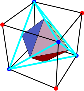
Figure 1: The octahedron represents the equivalence class of separable states. The set of points that lie outside the octahedron but inside the tetrahedron represent the equivalence class of entangled states. The set of points that lie outside the tetrahedron but inside the cube represent entanglement witnesses. The vertices of the tetrahedron represent the equivalence class of pure states. Points related by the tetrahedral symmetry represent the same equivalence class.

For describing notions, such as entanglement and witnesses, it is convenient to forget about the normalization of states. This allows one to describe the world of two qubits in three dimensions [28], as shown in Fig. 1. Interestingly, the same figure appears in various other contexts in quantum information theory. It first appeared in the Horodeckie‘s description [24] of 2 qubits with maximally mixed subsystems. It also appears in the characterization of the capacity of a single qubit quantum channel [41, 20, 26, 42, 54] and in other contexts [1, 49, 21, 45].

The 3 dimensional description, beautiful as it is, has weaknesses. One is that there are certain (fortunately, non-generic) states that do not seem to fit anywhere in Fig. 1. An example is the family of states where at least one subsystem is pure

$$({pure})_{A}\otimes({mixed})_{B},\quad({mixed})_{A}\otimes({pure})_{B},\quad({pure})_{A}\otimes({pure})_{B}$$ (1.1)

Another weakness is that the 3 dimensional figure gives no information on the measure of entanglement: The distance from the octahedron does not reflect any of the accepted measures of entanglement [39]. This is a consequence of the fact that the normalization of states does not matter in the 3 dimensional description.

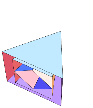
Figure 2: Four dimensional truncated cones describe the LSL equivalence classes of the of trace normalized witnesses, entangled and separable states. The cross section of the cones, here represented by nested rectangles, are the 3 dimensional polyhedra shown in Fig. 1. The largest cone is the cone of potential witnesses and the smallest cone is the dual cone of separable states. The intermediate cone is the self-dual cone of states. The distance from the cone of separable states is a measure of entanglement. The extraordinary families of Eq. (1.1) are represented by the apex of the cone.

To remedy this, we look at operations where the normalization of states matters. Specifically, we allow Alice and Bob to act on their qubits by matrices $M_{A,B}\in SL(2,\mathbb{C})$, the group of $2\times 2$ matrices, with complex entries and unit determinant. The interpretation of this family in terms of measurments shall be discussed in section 5. We shall call this class of operations LSL (for local, special and linear). LSL allows for a geometric description of the measure of entanglement. The price one pays is that one needs to go to 4 dimensions. The geometric picture that emerges is illustrated in Fig. 2, showing three nested cones. The largest cone is the cone of potential witnesses, whose cross section is the cube in Fig. 1. The boundary of the cone is special in that it is cohabited by two inequivalent families: The ordinary and the extraordinary. This makes it pathological . It may seem odd that the world of 2 qubits, which is a simple linear space in 16 dimensions, becomes pathological when viewed in terms of its equivalence classes. A useful analogy is the partitioning of (the connected) Minkowsky space-time to the (disconnected) equivalence classes of time-like, light-like and space-like vectors.

The four dimensional description is faithful to the measure of entanglement. More precisely, the concurrence, [51, 52], is the distance from the cone of separable states, the smallest nested cone. In particular, states represented by points near the apex of the cone have very little entanglement.

Many things will have to be left out. Among them: the notions of “entanglement of formation”, “entanglement cost” [6, 7, 18]; “bound entanglement” [22], “entanglement persistence” [10], multiparities entanglement, GHZ states [16] and the different entanglement measures [39]. Comprehensive reviews of entanglement, with extensive bibliography, are [55, 4, 25].

2 Bell states

The mothers of all entangled states are the four Bell states [9], commonly denoted by $\left|\beta_{\mu}\right\rangle$, here chosen to be

$${\sqrt{2}}\left|\beta_{0}\right\rangle={\left|00\right\rangle+\left|11\right\rangle}, {\sqrt{2}}\left|\beta_{1}\right\rangle={\left|00\right\rangle-\left|11\right\rangle}$$

$${\sqrt{2}}\left|\beta_{2}\right\rangle=\left|01\right\rangle+\left|10\right\rangle, i\sqrt{2}\left|\beta_{3}\right\rangle=\left|01\right\rangle-\left|10\right\rangle$$ (2.1)

The (isotropic) singlet is then $\left|\beta_{3}\right\rangle$. It is not a coincidence that the number of Bell states coincides with the number of Pauli matrices $\sigma_{\mu}$, (with $\sigma_{0}$ the identity).

Proposition 2.1.

The Pauli matrices give the unitary map from the computational basis, $\left|a\right\rangle\otimes\left|b\right\rangle$, with $a,b$ binary, to the Bell basis $\left|\beta_{\mu}\right\rangle,\ \mu\in\{0,1,2,3\}$. Explicitly:

$$\sqrt{2}\left|\beta_{\mu}\right\rangle=(\sigma_{\mu})_{ab}\left|a\right\rangle\otimes\left|b\right\rangle,\quad\sqrt{2}\left|a\right\rangle\otimes\left|b\right\rangle=(\sigma_{\mu}^{t})_{ab}\left|\beta_{\mu}\right\rangle$$ (2.2)

Summation over repeated indices is implied and the 4 Pauli matrices are chosen as

$$\sigma_{0}=\left(\begin{array}[]{cc}1&0\\ 0&1\\ \end{array}\right),\quad\sigma_{1}=\left(\begin{array}[]{rr}1&0\\ 0&-1\\ \end{array}\right),$$ (2.7)

$$\sigma_{2}=\left(\begin{array}[]{cc}0&1\\ 1&0\\ \end{array}\right),\quad\sigma_{3}=\left(\begin{array}[]{rr}0&-i\\ i&0\\ \end{array}\right).$$ (2.12)

Note that the anti-symmetric Pauli matrix is $\sigma_{3}$, (rather than the more common choice $\sigma_{2}$), a choice also made in [25].

Proposition 2.2.

The basic two-qubit operations, $\sigma_{\alpha}\otimes\sigma_{\beta}$, act on the Bell states as a permutation, (up to phase factors) and generate the the symmetry group of the tetrahedron.

Proof: From Eq. (2.2)

$$\sigma_{\alpha}\otimes\sigma_{\beta}\left|\beta_{\mu}\right\rangle=\frac{1}{\sqrt{2}}(\sigma_{\alpha}\sigma_{\mu}\sigma_{\beta}^{t})_{ab}\left|ab\right\rangle$$ (2.13)

Since

$$\sigma_{\mu}\sigma_{\nu}=\left\{\begin{array}[]{ll}i\epsilon_{\mu\nu k}\sigma_{k},&\hbox{$\mu,\nu,k\in\{1,2,3\}$;}\\ \sigma_{\mu},&\hbox{$\nu=0$;}\\ \sigma_{\nu},&\hbox{$\mu=0$.}\\ \end{array}\right.$$ (2.14)

We see that $\sigma_{\alpha}\otimes\sigma_{\beta}$ just permutes the Bell states (up to phase factors). Since $\sigma_{j}\otimes\sigma_{0}$ interchange $\left|\beta_{0}\right\rangle\leftrightarrow\left|\beta_{j}\right\rangle$, they generate the permutation group of the four Bell states, $S_{4}$. It is a fact that the tetrahedral group coincides with $S_{4}$. $\square$

The Bell projections play a key role in what we do.

Proposition 2.3.

The Bell projection $P_{\mu}=\left|\beta_{\mu}\right\rangle\left\langle\beta_{\mu}\right|$ (no summation over $\mu$, of course) have the form

$$4P_{0} = \sigma^{\otimes 2}_{0}+\sigma^{\otimes 2}_{1}+\sigma^{\otimes 2}_{2}-\sigma^{\otimes 2}_{3}\ ,$$

$$4P_{1} = \sigma^{\otimes 2}_{0}+\sigma^{\otimes 2}_{1}-\sigma^{\otimes 2}_{2}+\sigma^{\otimes 2}_{3}\ ,$$

$$4P_{2} = \sigma^{\otimes 2}_{0}-\sigma^{\otimes 2}_{1}+\sigma^{\otimes 2}_{2}+\sigma^{\otimes 2}_{3}\ ,$$ (2.15)

$$4P_{3} = \sigma^{\otimes 2}_{0}-\sigma^{\otimes 2}_{1}-\sigma^{\otimes 2}_{2}-\sigma^{\otimes 2}_{3}$$

where we denote

$$\sigma_{\mu}^{\otimes 2}=\sigma_{\mu}\otimes\sigma_{\mu}$$ (2.16)

Proof: From Eq. (2.2) one finds (no summation over $\mu$ below),

$$8P_{\mu}= = 4(\sigma_{\mu})_{ab}(\sigma_{\mu})_{dc}\left|a\right\rangle\left\langle c\right|\otimes\left|b\right\rangle\left\langle d\right|$$

$$= (\sigma_{\mu})_{ab}(\sigma_{\mu})_{dc}(\sigma_{\beta})_{ca}(\sigma_{\alpha})_{db}\,\sigma_{\beta}\otimes\sigma_{\alpha}$$

$$= Tr\,\big{(}\sigma_{\beta}\sigma_{\mu}\sigma_{\alpha}^{t}\sigma_{\mu}\big{)}\,\sigma_{\beta}\otimes\sigma_{\alpha}$$

In the second line we used

$$2\left|a\right\rangle\left\langle c\right|=Tr\big{(}\left|a\right\rangle\left\langle c\right|\sigma_{\beta}\big{)}\ \sigma_{\beta}=(\sigma_{\beta})_{ca}\sigma_{\beta}.$$ (2.18)

Since the Pauli matrices either commute or anti-commute, are either symmetric or antisymmetric, and are mutually orthogonal we have (no summation over $\mu$ here)

$$Tr\,\big{(}\sigma_{\beta}\sigma_{\mu}\sigma_{\alpha}^{t}\sigma_{\mu}\big{)}=\pm Tr\,\big{(}\sigma_{\beta}\sigma_{\alpha}^{t}\big{)}=\pm Tr\,\big{(}\sigma_{\beta}\sigma_{\alpha}\big{)}=\pm 2\delta_{\alpha,\beta}$$ (2.19)

Hence, only the diagonals survive in Eq. (2). $\square$

2.1 Teleportation

Bell states can be used to teleport [5] an unknown qubit. This is a consequence of the following teleportation lemma :

Lemma 2.4.

Let $\left|\psi\right\rangle$ be a single qubit pure state. Then the following identity holds

$$2\left|\psi\right\rangle\otimes\left|\beta_{\mu}\right\rangle=\left|\beta_{\nu}\right\rangle\otimes\left|\sigma_{\mu}^{t}\sigma_{\nu}\psi\right\rangle$$ (2.20)

Proof: From Eq. (2.2):

$$2\left|\psi\right\rangle\otimes\left|\beta_{\mu}\right\rangle = \sqrt{2}\psi_{c}(\sigma_{\mu})_{ab}\left|c\right\rangle\otimes\left|a\right\rangle\otimes\left|b\right\rangle$$

$$= \psi_{c}(\sigma_{\mu})_{ab}(\sigma_{\nu}^{t})_{ca}\left|\beta_{\nu}\right\rangle\otimes\left|b\right\rangle$$

$$= (\sigma_{\mu}^{t}\sigma_{\nu}\psi)_{b}\left|\beta_{\nu}\right\rangle\otimes\left|b\right\rangle$$

$$= \left|\beta_{\nu}\right\rangle\otimes\left|\sigma_{\mu}^{t}\sigma_{\nu}\psi\right\rangle\quad\quad\quad\quad\square$$

The identity has the following physical interpretation: The left hand side describes the situation where Alice has the (unknown) qubit $\left|\psi\right\rangle$ and shares with Bob the Bell state $\left|\beta_{\mu}\right\rangle$. The right hand side describes the superposition of the following situations: Alice pair of qubits is in one of the four Bell states while Bob’s qubit is a unitary transformation of $\left|\psi\right\rangle$. Alice can then measure in the Bell basis and tells Bob which Bell state she finds. Bob then performs the unitary operation $\sigma_{\nu}\sigma_{\mu}^{t}$ on his qubit to retrieve $\left|\psi\right\rangle$.

2.2 The CHSH Bell inequalities

The Bell states have the distinguished property that they give maximal violation of the CHSH Bell inequalities [13]. Bell inequalities [3] show that quantum mechanics can not be simulated by classical probability theory [2, 30, 35, 46, 19]. This bit of theory follows simply from the formulas above for the Bell projections, as we now outline.

Let us denote by $a_{1,2}$ the result of Alice measurement of $\sigma_{1,2}$ and by $b_{+,-}$ the result of Bob measurement of $(\sigma_{1}\pm\sigma_{2})/\sqrt{2}$. All these measurements are dichotomic and yield only $\pm 1$. Any assignment of $\pm 1$ to the corresponding 4 measurements yields

$$-2\leq a_{1}(b_{+}+b_{-})+a_{2}(b_{+}-b_{-})\leq 2$$ (2.22)

The same inequality must also hold on the average for any ensemble of classical systems. This is the CHSH Bell inequality[13, 34, 35].

Quantum mechanics is inconsistent with this inequality. To see this define the Bell operator [9] to be the observable corresponding to Eq. 2.22:

$$\mathbf{B} = \sigma_{1}\otimes\left(\frac{\sigma_{1}+\sigma_{2}}{\sqrt{2}}+\frac{\sigma_{1}-\sigma_{2}}{\sqrt{2}}\right)+\sigma_{2}\otimes\left(\frac{\sigma_{1}+\sigma_{2}}{\sqrt{2}}-\frac{\sigma_{1}-\sigma_{2}}{\sqrt{2}}\right)$$ (2.23)

$$= \sqrt{2}\big{(}\sigma^{\otimes 2}_{1}+\sigma^{\otimes 2}_{2}\big{)}=2\sqrt{2}\big{(}P_{0}-P_{3}\big{)}$$

Clearly, $\left|\beta_{0}\right\rangle,\ \left|\beta_{3}\right\rangle$ are eigenstates of $\mathbf{B}$ with eigenvalues $\pm 2\sqrt{2}$ and hence violate Eq. (2.22). The probabilistic aspect of quantum mechanics can not be attributed to a classical probabilistic source that prepares the qubits of Alice and Bob.

3 Separable states

In classical probability theory, random variables $x$ and $y$ are independent when their joint probability distribution is a product $P_{A}(x)P_{B}(y)$. Any joint probability distribution $P_{AB}(x,y)$ can be trivially written as a convex combination of product distributions:

$$P_{AB}(x,y)=\sum_{\alpha,\beta}P_{AB}(\alpha,\beta)\,\delta_{x,\alpha}\delta_{y,\beta}$$ (3.1)

where $P_{AB}(\alpha,\beta)$ are thought of as weights and the two delta functions as probability measures.

This is not true in quantum mechanics [19]. A state $\rho$, a positive matrix with unit trace, is the analog of a probability measure. A state of the form $\rho_{A}\otimes\rho_{B}$ describes the situation where Alice‘s and Bob‘s qubits are uncorrelated. However, it is not true that all states can be written as convex combinations of uncorrelated states. The states that can be written in this way are called separable [50, 25].

Definition 3.1.

A (normalized) state $\rho_{s}$ is separable if

$$\rho_{s}=\sum_{n=1}^{N}\,p_{n}\,{\rho}_{A}^{(n)}\otimes{\rho}_{B}^{(n)},$$ (3.2)

with $p_{n}\geq 0$ probabilities and $\rho^{(n)}_{A,B}$ positive operators with normalized trace. A state $\rho\geq 0$ which is not separable is entangled.

Clearly, the unnormalized separable states make a convex cone contained in the cone of all positive (unnormalized) states.

Separable states can be interpreted as mixtures of uncorrelated states where Alice and Bob rely on a common probability distribution, $p_{n}$ to create the mixture. This correlates Alice and Bob. Such correlation never violate Bell inequalities. For the CHSH this can be seen from the fact that for any product state

$$\left|Tr(\mathbf{B}\rho_{A}\otimes\rho_{B})\right|=\left|a_{1}(b_{+}+b_{-})+a_{2}(b_{+}-b_{-})\right|\leq|b_{+}+b_{-}|+|b_{+}-b_{-}|\leq 2$$

where now

$$|a_{1,2}|=|Tr(\sigma_{1,2}\rho_{A})|\leq 1,\quad|b_{+,-}|=\left|Tr\left(\frac{\sigma_{1}\pm\sigma_{2}}{\sqrt{2}}\rho_{B}\right)\right|\leq 1$$ (3.3)

This result extends to separable states by convexity.

States that violate a Bell inequality are necessarily entangled. However, there are lots of entangled states that do not violate any CHSH inequality. (The equivalence classes of states that satisfy the CHSH inequality and their visualization is given in [1].)

There are no known general conclusive tests of separability. However, for 2 qubits the Peres-Horodecki partial transposition test [36, 23] gives a simple spectral test of separability. To describe this test we first explain the notion of partial transposition for 2 qubits.

Any observable (Hermitian matrix) in the space of 2 qubits can be written as

$$A={\sf A}^{\mu\nu}\sigma_{\mu}\otimes\sigma_{\nu},\quad{\sf A}^{\mu\nu}\in\mathbb{R}$$ (3.4)

For reasons that shall become clear later we call ${\sf A}^{\mu\nu}$ the (contravariant) Lorentz components of $A$. The partial transpose of $A$, which we denote by $A^{P}$, is

$$A^{P}={\sf A}^{\mu\nu}\sigma_{\mu}\otimes\sigma_{\nu}^{t}=({\sf A}^{P})^{\mu\nu}\sigma_{\mu}\otimes\sigma_{\nu}$$ (3.5)

Observing that only $\sigma_{3}$ is anti-symmetric we see that the partial transpose, when expressed in terms of the Lorentz components, takes the form

$$({\sf A}^{P})^{\mu\nu}=\left\{\begin{array}[]{ll}{\sf A}^{\mu\nu},&\hbox{$\nu\neq 3$;}\\ -{\sf A}^{\mu\nu},&\hbox{$\nu=3$.}\\ \end{array}\right.$$ (3.6)

The Peres-Horodecki test is [36, 23]

Theorem 3.2.

A 2 qubit state $\rho\geq 0$ is separable iff $\rho^{P}\geq 0$

Proof: The “if” part is easy: If $\rho$ is separable, it can be written as in Eq. (3.2). Since $\rho_{B}\geq 0$ implies that also $\rho^{t}_{B}\geq 0$, one has that $\rho^{P}$, being a convex combination of positive operators, is also positive. The “only if” part requires more preparations. We shall give a simple geometric proof in section 11. $\square$

4 Witnesses

Witnesses are observables which can give evidence that a state is entangled. For our present purposes it is convenient to slightly widen this notion and to allow for witnesses which are in a sense trivial. We therefore define the cone of potential witnesses as follows:

Definition 4.1.

The dual cone to the cone of separable states shall be called the cone of potential witnesses. Explicitly, it is the collection of all observables $W$ such that

$$Tr({W}\rho_{s})\geq 0,$$ (4.1)

for all separable states $\rho_{s}$. We shall call $-Tr(W\rho)$ the (entanglement) evidence.

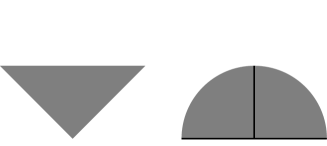
Figure 3: A cone with opening angle $\theta$ is dual to the cone with opening angle $\pi-\theta$. The quadrant, (left) is self-dual. The half-plane (right) is dual to the positive half-line. Here the usual scalar product of vectors corresponds to the trace in Eq. (4.1).

A potential witness is called simply a witness iff there exist some (necessarily entangled) state $\rho$ such that $Tr({W}\rho_{s})<0$. The witness then give conclusive evidence that $\rho$ is entangled. In fact by standard duality arguments [40] the definition implies

Proposition 4.2.

Any entangled state, $\rho$, has a witness $W$ giving positive evidence, i.e.

$$-Tr(W\rho)>0$$ (4.2)

The set of potential witnesses (unlike witnesses proper) is a convex set. A potential witness $W$ may not give positive evidence for any state $\rho$. Clearly, this will be the case whenever $W\geq 0$. Thus the cone of potential witnesses contains the cone of states:

$$Potential\ Witnesses\supset States\supset Separables$$ (4.3)

Observe that since $\rho=\mathbb{I}$ is clearly a separable (un-normalized) state it follows that any potential witness $W$ has $Tr\,W\geq 0$. Moreover, the following holds:

Theorem 4.3.

For any potential witness $W$, not identically zero,

$$Tr\,W>0.$$ (4.4)

In particular, witnesses, like states, may be normalized to have unit trace.

Proof: Note that the elements $\left\langle\varphi\otimes\psi\right|W\left|\varphi\otimes\psi\right\rangle$ suffice to determine all other matrix elements of $W$. This may be verified by considering the case ${\varphi\otimes\psi}=(\varphi_{1}+e^{i\alpha}\varphi_{2})\otimes(\psi_{1}+e^{i\beta}\psi_{2})$ for all $\alpha$’s and $\beta$’s. For any $W\neq 0$ one can therefore always find a normalized product state $\left|\varphi_{0}\right\rangle\otimes\left|\psi_{0}\right\rangle$ such that $\left\langle\varphi_{0}\otimes\psi_{0}\right|W\left|\varphi_{0}\otimes\psi_{0}\right\rangle>0$. Complete this to an orthonormal product base $\{\left|\varphi_{a}\right\rangle\otimes\left|\psi_{b}\right\rangle\}_{a,b=0,1}$. Since

$$Tr\,W=\left\langle\varphi_{a}\otimes\psi_{b}\right|W\left|\varphi_{a}\otimes\psi_{b}\right\rangle\,,$$ (4.5)

(summation implied), has no negative terms one concludes the strict inequality. $\square$

It remains to demonstrate that there indeed are entangled states or, equivalently, that the inequality Eq. (4.3) is strict. An example for a witness that is not a positive operator is the the swap, which exchanges the qubits of Alice and Bob:

$$S\left|\psi\right\rangle\otimes\left|\phi\right\rangle=\left|\phi\right\rangle\otimes\left|\psi\right\rangle$$ (4.6)

Proposition 4.4.

The swap has the following properties

1. $S$ is positive on separable states

2. $S=P_{0}+P_{1}+P_{2}-P_{3}$ gives positive evidence that the singlet is entangled

3. The swap is the partial transpose of a Bell projection: $S=2P_{0}^{P}$

Proof: That $S$ is positive on all pure product states follows from:

$${}_{A}\left\langle\psi\right|\otimes{}_{B}\left\langle\phi\right|S\left|\psi\right\rangle_{A}\otimes\left|\phi\right\rangle_{B}=\langle\psi|\phi\rangle_{A}\langle\phi|\psi\rangle_{B}=|\langle\psi|\phi\rangle|^{2}$$ (4.7)

It is then positive on all separable states by convexity and so belongs to the cone of potential witnesses. This proves 1. Part 2 follows by noting that the Bell states are eigenvectors of the swap. Part 3 follows from the observation that swap can be written as $S=\left|ab\right\rangle\left\langle ba\right|$, while $P_{0}=\mbox{$\frac{1}{2}$}\left|aa\right\rangle\left\langle bb\right|$. $\square$

It is, of course, not a coincidence that the swap is a witness of a Bell state. In Fig. 1 Bell states are represented by the (blue) dots at the vertices of the tetrahedron and the witnesses by the red dots at the corners of the cube obtained by reflection about the 3 axis. We shall see in Corollary 7.2 below, that the swap is, in fact, an optimal witness.

5 Equivalence and Local operations

We shall consider equivalence classes where $\rho$ and $\rho^{M}$ are considered equivalent provided

$$\rho\mapsto\rho^{M}=M\rho M^{\dagger},\quad M=M_{A}\otimes M_{B}$$ (5.1)

with $M_{A,B}$ taking values in the groups

$$SU(2)\subset SL(2,\mathbb{C})\subset GL(2,\mathbb{C})$$ (5.2)

The equivalence clearly preserve the positivity and the separability of states but, in general, not its normalization.

$M_{A,B}\in SL(2,\mathbb{C})$ will turn out to be our main tool and shall be designated by the acronym LSL for local, special (-unit determinant) and linear.

The linear maps in Eq. (5.1) with $M_{A,B}\in SL(2,\mathbb{C})$ or $GL(2,\mathbb{C})$ do not represent, in general, operations that Alice and Bob can perform on their qubits. Legitimate quantum operation are positivity preserving and trace non-increasing [35, 34]. This means that $M$ in Eq. (5.1) must satisfy $M^{\dagger}M\leq 1$. Quantum operation with $M^{\dagger}M<1$ are interpreted as a generalized measurement, aka POVM [14, 19, 35, 34, 8].

When $M_{A,B}\in SL(2,\mathbb{C})$ or $GL(2,\mathbb{C})$, $M^{\dagger}M\not\leq 1$ so the linear map in Eq. (5.1) do not represent legitimate quantum operations. Nevertheless with every such group element $M$ we can associate the bona-fide POVM element

$$M\mapsto\frac{M}{\|M\|}$$ (5.3)

The corresponding measurement filters [33, 11] the state

$$\rho\mapsto\frac{M\rho M^{\dagger}}{Tr(M\rho M^{\dagger})}$$ (5.4)

Filtering wastes a fraction of the qubits which Alice and Bob need to discard. Indeed, the filtration succeeds with probability

$$p(\rho)=\frac{Tr(M\rho M^{\dagger})}{\|M\|^{2}}\leq 1$$ (5.5)

(With $M_{A,B}\in SU(2)$ the “filtration” succeeds with probability one, but with $M_{A,B}\in SL(2,\mathbb{C}),GL(2,\mathbb{C})$ not.) Alice and Bob need to communicate over a classical channel, so they both keep only the qubits that pass the tests. This makes LSL a special case of SLOCC.

The equivalence classes introduced in Eq. (5.1) therefore admit the interpretation that two states are equivalent provided each can be filtered from the other and the filtration succeeds with finite probability. This imposes a restriction on what Alice and Bob are allowed to do. In particular, mixing is not an admissible operation. This is easily seen from the fact that $M$ preserve the rank of $\rho$ and so maps pure states to (unnormalized) pure states.

5.1 The equivalence classes of a single qubit

To appreciate the various notions of equivalence introduced above consider a single qubit. Any single qubit state $\rho$, can be identified with a (real) 4-vector ${\sf r}_{\mu}$

$$\rho={\sf r}^{\mu}\sigma_{\mu},$$ (5.6)

We shall refer to ${\sf r}^{\mu}$ as the (contravariant) “Lorentz components” of $\rho$. States admit the following simple geometric characterization:

Lemma 5.1.

The 4-vector ${\sf r}^{\mu}$ represents an (un-normalized) state iff it lies in the forward light-cone. Pure states are light-like. Normalized states lie on the time slice $t=\mbox{$\frac{1}{2}$}$.

Proof: This easily follows from

$$\det{\rho}={\sf r}^{\mu}{\sf r}^{\nu}\eta_{\mu\nu},\quad Tr{\rho}=2{\sf r}^{0}$$ (5.7)

where $\eta$ is the Minkowsky metric tensor, $\eta=diag(1,-1,-1,-1)$. Positivity $\rho>0$ requires that both the trace and determinant are non-negative. The 4-vector ${\sf r}^{\mu}$ must then lie in the forward light cone. A pure state, being rank one, has $\det\rho=0$ and is represented by a light-like vector. A normalized state has $Tr\rho=2{\sf r}^{0}=1$ and so lies on the fixed time-slice. $\square$

It follows from Eq. (5.7) that if ${\rho}^{M}=M{\rho}M^{\dagger}$, with $M\in SL(2,\mathbb{C})$ then the Lorentz component indeed transform like a vector under Lorentz transformation

$$\left({\sf r}^{M}\right)^{\mu}={(\Lambda_{M})^{\mu}}_{\nu}{\sf r}^{\nu}$$ (5.8)

where $\Lambda_{M}\in SO_{+}(1,3)$ is an (orthochronos) Lorentz transformation. If $M\in SU(2)$ then it just rotates the spatial part of the 4-vector.

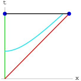
Figure 4: The light cone is represented by the diagonal (red) line. The equivalence classes of the $SU(2)$ (normalized) states are represented by the horizontal (black) line at fixed time. The $GL(2,\mathbb{C})$ equivalence classes are the two (blue) dots. The dot on the time axis represents the equivalence class of mixed states and the other, on the light cone, the pure states. The $SL(2,\mathbb{C})$ equivalence classes are represented by the vertical green line. Light-like vectors can be brought to this line only through infinite boost. Points representing the $SU(2)$ and $SL(2,\mathbb{C})$ equivalence classes that lie on the same interval, $t^{2}-x^{2}=const$, (cyan) have identical entropies.

It is instructive to compare the equivalence classes associated with normalized states of a single qubit with $M$ taking values in the three groups $SU(2),SL(2,\mathbb{C}),GL(2,\mathbb{C})$, shown in Fig. 4.

• $SU(2)$ acts as spatial rotations and can be used to map any normalized state to the $x-t$ plane at time slice $t=\mbox{$\frac{1}{2}$}$.

• $SL(2,\mathbb{C})$ acts as a Lorentz transformation and can be used to transform any time-like vector to the time-axis and any light-like vectors to any other light-like vector. This means that the LSL equivalence classes are represented by the semi-open interval $(0,\mbox{$\frac{1}{2}$}]$ and a point. It is natural to close the interval by gluing the point to the origin, (since a light-like vector can be transformed to the origin of the time axis in the limit of infinite boosts). The $SL(2,\mathbb{C})$ and $SU(2)$ equivalence classes of normalized one qubit states are then in 1-1 correspondence.

• The $GL(2,\mathbb{C})$ equivalence classes, however, are represented by two points: One representing all pure states (light-like vectors) and one representing all mixed states.

For a normalized qubit the von Neumann entropy, $H(\rho)=-Tr(\rho\log_{2}\rho)$, is uniquely determined by $\det\rho$. To see this express $\lambda$ be the large eigenvalue of $\rho$, as $2\lambda=1+\sqrt{1-4\det\rho}$. Then

$$H(\rho)=-h(\lambda)-h(1-\lambda),\quad h(\lambda)=\lambda\log_{2}\lambda\,.$$ (5.9)

Since $\det\rho$ is preserved by $SL(2,\mathbb{C})$ we see that LSL preserves the information on the entropy of the state (provided it is not renormalized). $GL(2,\mathbb{C})$ on the other hand, does not distinguish between mixed states with different entropies.

5.2 Equivalence classes of two qubit pure states

Two-qubits pure states are conveniently represented either in the computational basis or in the Bell basis:

$$\left|\psi\right\rangle=Y_{ab}\left|a\right\rangle\otimes\left|b\right\rangle=\xi^{\mu}\left|\beta_{\mu}\right\rangle,\quad\sqrt{2}\,Y=\xi^{\mu}\sigma_{\mu}$$ (5.10)

Summation over repeated indices is implied; $a,b\in\{0,1\}$ and $\mu\in\{0,1,2,3\}$. The state is normalized if $Tr\,(YY^{\dagger})=\xi_{\mu}\xi_{\mu}^{*}=1$. This means that the pure states are described by the seven-sphere $S^{7}$ [55, 32].

Local transformations take $\left|\psi\right\rangle$ to

$$M_{A}\otimes M_{B}\left|\psi\right\rangle=(M_{A}YM_{B}^{t})_{ab}\left|a\right\rangle\otimes\left|b\right\rangle$$ (5.11)

We see that $\det Y$ is invariant under the action of $M_{A,B}\in SL(2,\mathbb{C})$. As we shall see in the next section, $|\det Y|$ is a measure of the entanglement. This makes the entanglement an LSL invariant.

5.3 Entanglement distillation of pure states

The entanglement of a pure bi-partite normalized state is defined as the von Neumann entropy of either of its subsystems:

$$e(\left|\psi\right\rangle)=H(\rho_{A})=H(\rho_{B})$$ (5.12)

In the case at hand, where $\left|\psi\right\rangle$ is given by the matrix $Y$ of Eq. (5.10),

$$\rho_{A}=YY^{\dagger},\quad\rho_{B}=Y^{\dagger}Y.$$ (5.13)

It follows from Eq. (5.13) that

$$\det\rho_{A}=\det\rho_{B}=|\det Y|^{2}$$ (5.14)

By Eq. (5.9) $\det\rho_{A}$ determines the entropy of Alice’s qubit. It follows that the measure of entanglement is uniquely determined by $\det Y$. Moreover, since $\det Y$ is invariant under LSL by Eq. (5.11), we see that LSL is a useful equivalence not just for describing the notion of entanglement, but also for describing its measure.

One must distinguish between the (mathematical) fact that the information on the measure of entanglement is preserved under LSL and the (physical) principle that local operations dissipate entanglement [38]. The difference comes from the way both treat the issue of normalization. An an example, consider

$$\left|\psi_{\theta}\right\rangle=\cos\theta\left|00\right\rangle+\sin\theta\left|11\right\rangle,\quad 0\leq\theta\leq\pi/4$$ (5.15)

The LSL operation

$$M=\big{(}\sqrt{\tan\theta}\left|0\right\rangle\left\langle 0\right|+\sqrt{\cot\theta}\left|1\right\rangle\left\langle 1\right|\big{)}\otimes\mathbb{I}$$ (5.16)

filters from it the fully entangled unnormalized Bell state $\sqrt{\sin\theta\cos\theta}\left|\beta_{0}\right\rangle$. The information on the original measure of entanglement sits in the normalization. At the same time the corresponding quantum operation dissipates entanglement. By Eq. (5.5), the operation succeeds with probability

$$p(\left|\psi_{\theta}\right\rangle)=2\sin^{2}\theta$$ (5.17)

Using the fact $e(\left|\beta_{0}\right\rangle)=1$ one ends up with less entanglement:

$$p(\left|\psi_{\theta}\right\rangle)=p(\left|\psi_{\theta}\right\rangle)e(\left|\beta_{0}\right\rangle)\leq e(\left|\psi_{\theta}\right\rangle)$$ (5.18)

in accordance with the principle that local operations dissipate entanglement, see Fig. 5.

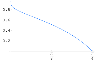
Figure 5: The relative dissipation of the entanglement, $(e-p)/e$, for filtering Bell states from the states in Eq. (5.15) as a function of $\theta$. The entanglement is $e$ and the probability of filtering a Bell state is $p$. The graph expresses the inequality in Eq. (5.18).

6 Duality of states and observables

6.1 Contragradient actions

States $\rho$ and observables $W$ naturally live in dual spaces since pairing the two, $Tr\,(\rho W)$, gives a number. It is both natural and convenient to define the operations so that they act on states and witnesses in a way that respects their duality. Namely:

$$\rho\mapsto\rho^{M} = M^{\dagger}\rho M$$

$$W\mapsto W^{M} = M^{-1}W(M^{-1})^{\dagger}$$ (6.1)

If $M$ is unitary, $M^{-1}=M^{\dagger}$, then states and observables transform the same way, but when $M$ is only invertible, they do not. With this choice $\rho W$ undergoes a similarity transformation

$$\rho W\mapsto\rho^{M}(W)^{M}=M^{\dagger}\,(\rho W)\,(M^{\dagger})^{-1}$$ (6.2)

and $Tr(\rho W)$ is invariant.

When the local operations are taken from $SL(2,\mathbb{C})$, there is a map, the tilde map, that takes observables to states and vice versa. By this we mean that if $A$ transforms as a state then $\tilde{A}$ transforms as an observable, i.e.

$$\widetilde{(M^{\dagger}AM)}=M^{-1}\,\tilde{A}\,(M^{-1})^{\dagger}$$ (6.3)

For a single qubit the tilde map is given by

$$\tilde{A}=\sigma_{3}A^{t}\sigma_{3}$$ (6.4)

and for a pair of qubits by

$$\tilde{A}=(\sigma_{3}\otimes\sigma_{3})\,A^{t}\,(\sigma_{3}\otimes\sigma_{3})$$ (6.5)

That the tilde map indeed satisfies Eq. (6.3) is a property of $SL(2,\mathbb{C})$. It follows from the identity

$$\sigma_{3}M^{t}\sigma_{3}=M^{-1},\quad M\in SL(2,\mathbb{C})$$ (6.6)

The tilde operation acts on the Pauli spin matrices as “spin-flip”, reversing the spatial component ,

$$\tilde{\sigma}_{\mu}=\sigma_{3}\sigma^{t}_{\mu}\sigma_{3}=\sigma^{\mu}$$ (6.7)

(Indices are raised and lowered according to the Minkowsky metric tensor $\eta$). It follows that

$$Tr\,(\sigma_{\mu}\tilde{\sigma}_{\nu})=2\eta_{\mu\nu}$$ (6.8)

If we represent single qubit states and observables by contravariant components of 4-vectors,

$$\rho={\sf r}^{\mu}\sigma_{\mu},\quad W={\sf w}^{\mu}\tilde{\sigma}_{\mu}$$ (6.9)

the invariance of $Tr(\rho{W})$ implies that ${\sf r}^{\mu}$ and ${\sf w}^{\mu}$ transform under the same Lorentz transformation:

$$Tr(\rho{W})=2\,{\sf r}^{\mu}{\sf w}^{\nu}\eta_{\mu\nu}$$ (6.10)

This carries over to 2-qubits where states and witnesses are represented by contravariant tensors

$$\rho={\sf r}^{\mu\nu}\sigma_{\mu}\otimes\sigma_{\nu},\quad W={\sf W}^{\mu\nu}\tilde{\sigma}_{\mu}\otimes\tilde{\sigma}_{\nu}$$ (6.11)

and now the Lorentz scalar is

$$Tr(\rho{W})=4\,{\sf r}^{\mu\nu}{\sf W}_{\mu\nu}$$ (6.12)

6.2 Self-duals and Anti-self-duals

We shall say that $W_{e}$ is self-dual if

$$W_{e}=\tilde{W}_{e}$$ (6.13)

For a single qubit self-duality means that the state is fully mixed. For 2-qubits it readily follows from Eq. (6.7) that the matrix of Lorentz components of $W_{e}$ has the form

$${\sf W}_{e}=\left(\begin{array}[]{cccc}{\sf W}_{00}&0&0&0\\ 0&{\sf W}_{11}&{\sf W}_{12}&{\sf W}_{13}\\ 0&{\sf W}_{21}&{\sf W}_{22}&{\sf W}_{23}\\ 0&{\sf W}_{31}&{\sf W}_{32}&{\sf W}_{33}\\ \end{array}\right)$$ (6.14)

The space of self-duals is then evidently 10 dimensional. Self-dual states represent fully mixed subsystems. Self-dual observables are time-reversal invariant.

Since $SU(2)$ act on the (spatial components) of the Pauli matrices like a rotation, the singular value decomposition implies that

Proposition 6.1.

Every self-dual $W_{e}$ can be brought to a canonical form

$$W_{e}\to{\sf w}_{\mu}\sigma_{\mu}^{\otimes 2}=\omega_{\mu}P_{\mu}$$ (6.15)

by a pair of $SU(2)$ transformation, where ${\sf w_{0}}={\sf W}_{00}$ and the spatial components, ${\sf w}_{j}$ are the singular values of the $3\times 3$ sub-matrix of ${\sf W}_{e}$ (up to sign). The $\omega_{\mu}$ and ${\sf w}_{\mu}$ are related by the linear transformation of Eq. (2.3)

$$\left(\begin{array}[]{c}\omega_{0}\\ \omega_{1}\\ \omega_{2}\\ \omega_{3}\end{array}\right)=\left(\begin{array}[]{crrr}1&1&1&-1\\ 1&1&-1&1\\ 1&-1&1&1\\ 1&-1&-1&-1\\ \end{array}\right)\left(\begin{array}[]{c}{\sf w}_{0}\\ {\sf w}_{1}\\ {\sf w}_{2}\\ {\sf w}_{3}\end{array}\right)$$ (6.28)

In particular, the $\omega_{\mu}$ are all real.

The space of (not necessarily hermitian) anti-self-dual operators may be identified with the Lie algebra of $SL(2,\mathbb{C})\otimes SL(2,\mathbb{C})$. Indeed by Eq. (6.6)

$$\tilde{M}=M^{-1},\quad\forall M\in SL(2,\mathbb{C})\otimes SL(2,\mathbb{C})$$ (6.29)

from which follows

$$\delta\tilde{M}=-M^{-1}\,(\delta M)\,M^{-1}$$ (6.30)

The Lie algebra is the variation at the identity where $\delta\tilde{M}=-\delta M$, i.e. the Lie algebra is anti-self-dual. Since the linear space of anti-self-dual operators is 6-complex-dimensional (spanned by $\sigma_{i}\otimes 1,\,1\otimes\sigma_{i};\;i=1,2,3$) it must coincide with the whole Lie algebra.

6.3 LSL invariants

Since $\tilde{A}$ transform contragradiently to $A$, the product $\tilde{A}A$ undergoes a similarity transformation by Eq. (6.2). This allows us to associate spectral invariants with the LSL action:

Lemma 6.2.

For any (n-qubit) observable, the spectrum of $\tilde{A}A$ and $\det A$ are LSL invariants.

To get a feeling for the invariants consider first the case of a single qubit state $\rho={\sf r}^{\mu}\sigma_{\mu}$. In this case there is just a single invariant

$$\tilde{\rho}\rho=({\sf r}_{\mu}{\sf r}^{\mu})\,\mathbb{I}=(\det\rho)\,\mathbb{I}$$ (6.31)

By Eq. (5.9) the determinant encodes the information on the entropy of the (normalized) state and vanishes for pure states.

Multi-qubits observables of the form $\rho=\rho_{A}\otimes\rho_{B}$ then have as invariant $\det(\rho_{A})\det(\rho_{B})$. In particular, it follows that

$$\tilde{\rho}\rho=0$$ (6.32)

whenever either $\rho_{A}$ or $\rho_{B}$ is a pure state.

In the case of two qubits, $spec(\tilde{A}A)$ gives four LSL-invariants. The invariant $\det A$ is closely related to them, since

$$\det(\tilde{A}A)=(\det A)(\det\tilde{A})=(\det A)^{2}$$ (6.33)

Thus the only additional information supplied by $\det A$ is its sign.

In the particular case where $A$ is a state we trivially have $\det A\geq 0$. As $\tilde{\rho}\rho$ is readily seen to be similar to the positive operator

$$\sqrt{\rho}\,\tilde{\rho}\sqrt{\rho},$$ (6.34)

one evidently has in this case

Lemma 6.3.

(Wootters [51]) When $\rho>0$ the eigenvalues of $\tilde{\rho}\rho$ are all positive.

We define the LSL invariant spectrum of state $\rho$ as the the positive roots of the eigenvalues of $\tilde{\rho}\rho$.

Since a witness $W$ is, in general, not positive, it is not a-priori clear that eigenvalues of $\tilde{W}W$ are positive. In fact, for a general observable $A$, the spectrum of $\tilde{A}A$ need not even be real. We shall see, in the next section, that for witnesses the eigenvalues of $\tilde{W}W$ are still positive. Moreover, as we shall see, there is a natural way to choose signs for the roots of these eigenvalues in a way that is consistent with the invariance of $\det W$. This will allow defining the LSL invariant spectrum of $W$ in a way that amalgamate the two invariants of lemma 6.2.

7 Canonical forms as optimizers

We want to extend the notion of LSL invariant spectrum to witnesses. Since witnesses are, in general, not positive, the argument leading to lemma 6.3 does not apply. However, as we shall see, the LSL invariant spectrum $\{\omega_{\mu}\}$ is still well defined and real. In fact the following key result holds:

Theorem 7.1.

Any observable $W$ in the interior of the cone of potential witnesses is LSL equivalent to a witness of canonical form

$$W\mapsto\omega_{\mu}P_{\mu}$$ (7.1)

where $P_{\mu}$ are the Bell projections, $\omega_{\mu}\in\mathbb{R}$, and $\omega_{\mu}^{2}$ are the eigenvalues of $\tilde{W}W$. The representation (7.1) is unique, up to permutations of the $\omega_{\mu}$’s. This generate the tetrahedral group manifest in the Fig. 1. A unique representation is obtained by imposing the canonical order

$$\omega_{0}\geq\omega_{1}\geq\omega_{2}\geq|\omega_{3}|$$ (7.2)

In particular, at most one LSL-eigenvalue, the one with smallest magnitude, is negative.

The upshot of this theorem is that the LSL equivalence classes of the 16 dimensional cone of potential witnesses, and therefore also the cone of (un-normalized) states, can be represented by points in $\mathbb{R}^{4}$.

The proof of this theorem depends on a variational principle. Specifically on finding a witness that maximizes the entanglement evidence, in the sense of definition 4.1. This point of view leads to our second key result:

Theorem 7.2.

Let $W$ and $\rho$ be in the interior of the cone of potential witnesses, and let $W_{e}=\omega_{\mu}P_{\mu}$ and $\rho_{e}=\rho_{\mu}P_{\mu}$ be their associated canonical forms. Then

$$\min_{M}\left\{Tr(W^{M}\rho)\right\}=Tr(W_{e}\rho_{e})=\sum_{\mu}\rho_{\mu}\omega_{\mu}$$ (7.3)

where $\rho_{\mu}$ are chosen in canonical order, Eq. (7.2), while $\omega_{\mu}$ are chosen with the anti-canonical order

$$\omega_{0}\leq\omega_{1}\leq\omega_{2}\leq\omega_{3}$$ (7.4)

In particular, taking $\rho=1$, we see that the LSL map $W\mapsto\omega_{\mu}P_{\mu}$ is trace decreasing.

Corollary 7.3.

It follows that to test whether a state is entangled it is enough to test its canonical representer against canonical witnesses.

The proofs of both theorems are given in the following subsections.

7.1 Existence of the optimizer

Consider the stationary points of the function $M\mapsto Tr(\rho W^{M})$ where $M=M_{A}\otimes M_{B}$. For $M_{A,B}\in SU(2)$, this function must have (finite) maximum and minimum since $SU(2)$ is compact. However, in the case that $M_{A,B}\in SL(2,\mathbb{C})$, which is not compact, there may be no stationary point for any finite $M$. The existence of a minimum is guaranteed by the following lemma.

Lemma 7.4.

Suppose $\rho$ and $W$ both lie in the interior of the cone of potential witnesses, i.e. satisfying a strict inequality in (4.1). Then, the function $Tr\left(\rho W^{M}\right)$, diverges to $+\infty$ as either $M_{A}\in SL(2,\mathbb{C})$ or $M_{B}\in SL(2,\mathbb{C})$ go to infinity. In particular, it has a finite minimizer.

The lemma may be written in a more symmetric form (under $\rho\leftrightarrow W$) by noting

$$Tr(\rho^{M}W^{N})=Tr(\rho W^{(M^{-1})^{\dagger}N}).$$ (7.5)

Sketch of the proof: The spectrum of any $M_{A}\in SL(2,\mathbb{C})$ is of the form $\{\lambda,1/\lambda\}$. The element is large when $|\lambda|$ is large. It can then be approximated by a rank one operator (corresponding to the large eigenvalue) $M_{A}\simeq\lambda P$, with $P$ a one dimensional projection. Thus $M=M_{A}\otimes M_{B}\simeq\lambda P\otimes M_{B}$ is essentially supported on a $1\otimes 2$ dimensional subspace of the full $2\otimes 2$ space. As a $1\otimes 2$ space cannot support any entanglement, the corresponding expectation $Tr\left(\rho W^{M}\right)\simeq|\lambda|^{2}Tr\left(\rho W^{P\otimes M_{B}}\right)$ must be positive. As it is multiplied by $|\lambda|^{2}$ it actually diverge to $+\infty$ with $\lambda$. $\square$

An alternative proof of lemma 7.4 and a generalization of it which applies to witness on the boundary are described in appendix A.

7.2 Characterization of the optimizer

In the previous section we have seen that $Tr(\rho W^{M})$ has a minimizer. Once its existance is guaranteed, one may use standard variational procedure to characterize it. As we shall show whenever $\rho$ is of the canonical form the minimizer—the optimal witness, is also of the form $\omega_{\mu}P_{\mu}$.

Note that the Bell projections are self-dual, $P_{\mu}=\tilde{P}_{\mu}$. We start by showing that the stationary points of $Tr(\rho W^{M})$ are self-dual.

Lemma 7.5.

The stationary points of the function $Tr(\rho W^{M})$, where $M=M_{A}\otimes M_{B}$ with $M_{A,B}\in SL(2,\mathbb{C})$ are the self-dual points, i.e.

$$\widetilde{\rho W^{M}}=\rho W^{M}$$ (7.6)

Proof: Suppose $Tr(\rho W^{M})$ is stationary at the identity $M=I$ then for any small LSL-variation $M=I+\delta M$ we must have

$$0 = \delta Tr(\rho W^{M})=\delta Tr(\rho M^{-1}W{M^{-1}}^{\dagger})$$

$$= Tr\left(\rho(-\delta M)W+\rho W(-\delta M^{\dagger})\right)$$

$$= -Tr(W\rho\delta M)-Tr(W\rho\delta M)^{*}$$

$$= -2Re\,Tr(W\rho\delta M)$$

where we used the fact that $\rho,W$ are hermitian. Recall that by Eq. (6.29) the Lie algebra of LSL consists of complex matrices satisfying $\tilde{\delta M}=-\delta M$. Stationarity requires $W\rho$ to be in the space orthogonal to these which is the space of self-duals $W\rho=\widetilde{W\rho}$. Formally this follows by using the identity $Tr(\tilde{A}\tilde{B})=Tr(AB)$ to write

$$0=\delta Tr(\rho W^{M})=-Re\,Tr\bigg{(}\delta M\,\big{(}W\rho-\widetilde{W\rho}\big{)}\bigg{)}$$ (7.8)

As both $\delta M$ and $W\rho-\widetilde{W\rho}$ are anti-self dual, the trace of their product vanishes for arbitrary (complex) anti self-dual $\delta M$ if and only if $W\rho=\widetilde{W\rho}$. A stationary point at arbitrary $M$ similarly lead to (7.6). $\square$

It follows that any strict potential witness $W$ is LSL-equivalent to a self-dual one. To see this take $\rho=1$. Lemma 7.4 then guarantees that $Tr({W}^{M})$ has a minimum, and lemma 7.5 tells us that the minimizer ${W}^{M}$ is self dual. Moreover, by applying Prop. 6.1 it follows that $W$ can be brought to a canonical form, Eq. (7.1). The lemma below gives a direct proof of this fact without relying on the singular value decomposition used in Prop. 6.1.

Lemma 7.6.

Suppose the state $\rho$ is self-dual, then $Tr(\rho W^{M})$ has its stationary points where $[\rho^{2},W^{M}]=0$. In particular if $\rho$ is in canonical form Eq. (7.1), then (at least in the generic non-degenerate case) so is the minimizer ${W}^{M}$. In the case of degenerate $\rho^{2}$ the minimizer ${W}^{M}$ is not unique but may still be chosen as canonical.

Proof: Combining $\rho=\tilde{\rho}$ with the minimizer condition (7.6) gives

$$(\rho W^{M})=\widetilde{(\rho W^{M})}=\widetilde{(W^{M})}\tilde{\rho}=\widetilde{(W^{M})}\rho$$ (7.9)

and similarly

$$(W^{M}\rho)=\widetilde{(W^{M}\rho)}=\tilde{\rho}\widetilde{(W^{M})}=\rho\widetilde{(W^{M})}$$ (7.10)

Combining the two gives $\rho^{2}W^{M}=W^{M}\rho^{2}$. Thus the Bell basis which diagonalize $\rho$ must do the same for $W^{M}$, unless $\rho^{2}$ happens to be degenerate. In the special case of degenerate $\rho^{2}$ one may find a Bell-diagonalized minimizer $W^{M}$ by considering first a small degeneracy breaking perturbation of $\rho$. $\square$

7.3 Proofs of the two theorems

Proof of theorem 7.1: Choosing some generic $\rho$ of the canonical form (7.1) and arbitrary $W$, we are guaranteed by lemma 7.4 that $Tr(\rho{W}^{M})$ has a minimum. Lemma 7.6 then tells us that the minimizer $W^{M}$ is also of the canonical form $\omega_{\mu}P_{\mu}$. The four eigenvalues $\omega_{\mu}$ can be permuted arbitrarily by Proposition 2.2.

The LSL invariance of

$$Spec(\tilde{W}W)=\{\omega_{\mu}^{2}\}$$ (7.11)

determines $\omega_{\mu}$ up to sign. To determine the signs we shall show that at most one LSL-eigenvalue is negative. To this end, note first that from any pair of the Bell states, one may consruct a separable state $\left|\beta_{\mu}\right\rangle+e^{i\varphi}\left|\beta_{\nu}\right\rangle$ (actually $e^{i\varphi}=1$ or $i$). E.g.

$$\left|\beta_{0}\right\rangle+\left|\beta_{1}\right\rangle=\sqrt{2}\left|00\right\rangle,\;\left|\beta_{2}\right\rangle+i\left|\beta_{3}\right\rangle=\sqrt{2}\left|01\right\rangle,etc$$ (7.12)

(Since local unitaries can permute Bell states, similar relations must hold for all other Bell pairs.) With $W$ in canonical form we then have by Eq. (4.1) that

$$0\leq\left\langle\beta_{\mu}+e^{-i\varphi}\beta_{\nu}\right|W^{M}\left|\beta_{\mu}+e^{i\varphi}\beta_{\nu}\right\rangle=(\omega_{\mu}+\omega_{\nu}),\quad\mu\neq\nu$$ (7.13)

This imply that at most one of the eigenvalues is negative, and moreover, it must be the one of smallest absolute value. The LSL-invariance of $\det(W)$ then fixes the signs of all the $\omega_{\mu}$ uniquely. The proof is complete. $\square$

Proof of theorem 7.2: Given $W$ and $\rho$ theorem 7.1 tells us that that $\rho^{N}=\rho_{e}=\rho_{\mu}P_{\mu}$ for some $N\in SL(2,\mathbb{C})\otimes SL(2,\mathbb{C})$. We therefore have

$$Tr(\rho{W})=Tr(\rho_{e}^{N^{-1}}{W})=Tr(\rho_{e}{W}^{N})\geq\min_{M}\left\{Tr(\rho_{e}{W}^{M})\right\}$$ (7.14)

By lemma 7.6 we know that $Tr(\rho_{e}{W}^{M})$ is stationary whenever ${W}^{M}=\omega_{\mu}P_{\mu}$. The minimum clearly corresponds to requiring Eqs. (7.2,7.4). $\square$

7.4 The boundary of the cone of witnesses

Theorem 7.1 applies only to observables $W$ in the interior of the cone of potential witnesses. It can be extended to to the boundary, provided the notion of LSL-transformations is appropriately modified. We shall say that observable $B$ is obtained by a generalized LSL-transformation from observable $A$ iff it is in the closure of the equivalence class of $A$ , i.e. iff there exist a series $\{M_{i}\}_{i=1}^{\infty}\subset SL(2,\mathbb{C})\otimes SL(2,\mathbb{C})$ such that $A^{M_{i}}\rightarrow B$. Theorems 7.1,7.2 then hold for any potential witness with $\min_{M}$ replaced by $\inf_{M}$. The proof follows very similar lines to the proofs given above. The only major change is replacing lemma 7.4 by a generalization of it described in the appendix A.

8 Classification: A Lorentzian picture

8.1 Geometric characterization of witnesses

The matrix of Lorentz components ${\sf W}_{\mu\nu}$ of a potential witness $W$, Eq. (6.11), allows for a simple geometric characterization of potential witnesses. By definition, a potential witness has positive expectation for product states,

$$0\leq Tr\,({W}{\rho}_{A}\otimes{\rho}_{B})=4\,{\sf W}_{\mu\nu}\,(\rho_{A})^{\mu}(\rho_{B})^{\nu}.$$ (8.1)

Since the 4-vectors $\left(\rho_{A,B}\right)_{\mu}$ can lie anywhere in the forward light cone (by lemma 5.1), we learn that the matrix ${\sf W}$ maps the forward light cone into itself. Points that lie in the interior of the cone of potential witnesses satisfy a strict inequality in Eq. (8.1). The map ${\sf W}$ then sends the forward light cone into its (timelike) interior.

8.2 Lorentz singular values

By Eq. (5.8) LSL acts on the Lorentz components of a 2-qubit observable $W$ by a pair of Lorentz transformations

$${\sf W}^{A\otimes B}=\Lambda_{A}\,{\sf W}\,\Lambda_{B}^{t}$$ (8.2)

where $\Lambda_{A,B}\in SO_{+}(1,3)$ are two $4\times 4$ Lorentz transformation matrices.

From Eq. (2.3) it follows that if $W$ is in canonical form then

$$W=\omega_{\mu}P_{\mu}={\sf w}_{\mu}\sigma_{\mu}^{\otimes 2}$$ (8.3)

so that the Lorentz matrix ${\sf W}$ is diagonal. The $\omega_{\mu}$ and ${\sf w}_{\mu}$ coordinates are related by Eq. (6.28).

Thus when viewed in terms of Lorentzian components, bringing $W$ to its canonical form consists of diagonalizing the associated tensor ${\sf W}_{\mu\nu}$ by a pair of Lorentz transformations. This is reminiscent of the notion of the singular decomposition of a matrix (which is defined in the same way with the Lorentz transformation replaced by orthogonal matrices).

For a matrix $M$ its singular values are the (positive) roots of the matrix $M^{\dagger}M$. The Lorentzian analog of $M^{\dagger}M$ turns out to be the matrix ${\sf W}^{\lambda\mu}{\sf W}_{\lambda\nu}$. It is convenient to write it as ${\sf W}^{\star}{\sf W}$ where the ‘Lorentz conjugated matrix’ is defined by

$${\sf W}^{\star}=\eta{\sf W}^{t}\eta$$ (8.4)

One readily verifies that componentwise

$$({\sf W}^{\star})_{\mu\nu}={\sf W}^{\nu\mu}$$ (8.5)

Since Lorentz transformations leave the Minkowsky metric invariant, $\Lambda^{t}\eta\Lambda=\eta$, one has

$$\Lambda^{\star}=\Lambda^{-1}$$ (8.6)

It then follows that under (8.2) ${\sf W}^{\star}{\sf W}$ undergoes a similarity transformation

$${\sf W}^{\star}{\sf W}\to\big{(}\Lambda_{M}{\sf W}\Lambda_{N}^{t}\big{)}^{\star}\big{(}\Lambda_{M}{\sf W}\Lambda_{N}^{t}\big{)}=(\Lambda_{N}^{t})^{-1}\big{(}{\sf W}^{\star}{\sf W}\big{)}\Lambda_{N}^{t}$$ (8.7)

and similarly for ${\sf W}{\sf W}^{\star}$. The spectra of ${\sf W}^{\star}{\sf W}$ and ${\sf W}{\sf W}^{\star}$ are therefore LSL invariant.

The LSL invariance of the spectrum of ${\sf W}{\sf W}^{\star}$ does not depend on $W$ being a witness. In general, this spectrum is complex. For matrices that lie in the cone of witnesses one has, by Eq. (8.3), that the eigenvalues of ${\sf W}{\sf W}^{\star}$ are ${\sf w}_{\mu}^{2}$ and are positive (or zero). In this case, in analogy with the notion of singular values, one may define the Lorentz singular values as $|{\sf w}_{\mu}|$.

Remark 8.1.

Diagonal Lorentz transformations in $O(1,3)$ with $\pm 1$ on the diagonal, bring any diagonal $W$ to a positive diagonal form. However, we are allowed only proper orthochronos Lorentz transformations, $SO_{+}(1,3)$. Thus the canonical coordinates ${\sf w}_{\mu}$ defined via Eq.  (8.3) may differ in signs from the (positive) Lorentz singular values.

8.3 Tetrahedral symmetry and fundamental domains

The tetrahedral group acts on the coordinates $\omega_{\mu}$ as permutations. In terms of the coordinates ${\sf w}_{\mu}$ this group acts as permutations and sign flips of the three ‘spatial’ coordinates ${\sf w}_{j}$ which leave $sgn({\sf w}_{1}{\sf w}_{2}{\sf w}_{3})$ invariant. To see this note first that the relation $4{\sf w}_{0}=\omega_{0}+\omega_{1}+\omega_{2}+\omega_{3}>0$ shows that ${\sf w}_{0}$ is independent of the ordering of $\omega_{\mu}$. Hence, the tetrahedral group acts only on the spatial components ${\sf w}_{j}$. For proper Lorentz transformations $\det({\sf W})={\sf w}_{0}{\sf w}_{1}{\sf w}_{2}{\sf w}_{3}$ cannot change sign. In cases when $\det({\sf W})>0$ the canonical coordinates may be taken as equal to the Lorentz singular values. If $\det({\sf W})<0$ then at least one of the canonical coordinates (which we will usually take to be the one having least absolute value) must be chosen as negative. The tetrahedral symmetry allows one to impose ${\sf w}_{\mu}$ to be in the fundamental domain

$${\sf w}_{1}\geq{\sf w}_{2}\geq|{\sf w}_{3}|$$ (8.8)

which is equivalent to Eq. (7.2). The antipodal fundamental domain

$$-{\sf w}_{1}\geq-{\sf w}_{2}\geq|{\sf w}_{3}|$$ (8.9)

is equivalent to the anti-canonical ordering of Eq. (7.4).

8.4 Classification of potential witnesses

Symmetric matrices that map the forward light-cone into itself may be interpreted in general relativity as energy-momentum tensors that satisfy the “dominant energy condition”. Their classification is given in p. 89-90 in [17]. We need a generalization of this classification to non-symmetric matrices where we are allowed to use a pair of Lorentz transformations as in Eq. (8.2). The classification is given in [48] and is based on [15]:

Theorem 8.2.

Let ${\sf W}$ be a $4\times 4$ matrix that maps the forward light-cone into itself. Fix arbitrary $\kappa>0$. Then there is a pair of Lorentz transformations $\Lambda_{A},\Lambda_{B}$ such that $\Lambda_{A}{\sf W}\Lambda_{B}$ is of one of the 4 canonical forms, unique subject to Eq. 8.8:

• The ordinary diagonal form

  $$\left(\begin{array}[]{cccc}{\sf w}_{0}&0&0&0\\ 0&{\sf w}_{1}&0&0\\ 0&0&{\sf w}_{2}&0\\ 0&0&0&{\sf w}_{3}\\ \end{array}\right),$$ (8.10)

  associated with the cone in 4 dimensions with a cross section that is a 3 dimensional cube:

  $$\quad{\sf w}_{0}\geq|{\sf w}_{j}|$$ (8.11)

• The first extraordinary form

  $$\left(\begin{array}[]{cccc}{\sf w}_{0}+\kappa&-\kappa&0&0\\ \kappa&{\sf w}_{1}-\kappa&0&0\\ 0&0&{\sf w}_{2}&0\\ 0&0&0&{\sf w}_{3}\\ \end{array}\right),$$ (8.12)

  associated with the boundary of the cone

  $${\sf w}_{0}={\sf w}_{1}\geq|{\sf w}_{2,3}|$$ (8.13)

• The second extraordinary form

  $$\left(\begin{array}[]{cccc}\kappa&\kappa&0&0\\ 0&0&0&0\\ 0&0&0&0\\ 0&0&0&0\\ \end{array}\right)$$ (8.14)

  associated with the apex of the cone ${\sf w}_{\mu}=0$.

• The third extraordinary form

  $$\left(\begin{array}[]{cccc}\kappa&0&0&0\\ \kappa&0&0&0\\ 0&0&0&0\\ 0&0&0&0\\ \end{array}\right),$$ (8.15)

  also associated with the apex of the cone ${\sf w}_{\mu}=0$.

${\sf w}_{\mu}$, the “Lorentz singular values”, are roots of the eigenvalues of $W^{\star}W$.

The proof of this theorem is given in appendix B.

9 The Geometry of witnesses and states

We have seen that the LSL equivalence classes of witnesses, states and separable states are represented by nested cones in four dimensions. In this section we give a geometric description of these cones.

9.1 The geometry of ordinary witnesses

A diagonal witness

$$W_{e}={\sf w}_{\mu}\sigma_{\mu}^{\otimes 2}$$ (9.1)

maps the light cone into itself iff ${\sf w}_{0}\geq|{\sf w}_{j}|$. The LSL equivalence classes of the (ordinary) potential witnesses are therefore characterized geometrically by the cone in 4 dimensions:

$${\sf w}_{0}\geq|{\sf w}_{1}|,|{\sf w}_{2}|,|{\sf w}_{3}|$$ (9.2)

whose cross section is the cube.

By theorem 7.2 the canonical representative of a witness also minimizes $Tr(W^{M})$. Thus the representatives of normalized witnesses have ${\sf w}_{0}\leq\mbox{$\frac{1}{4}$}$ giving a capped cone. All points in the capped cone are relevant since given $W_{e}\neq 0$ with $Tr\ W_{e}<1$ one easily finds $M$ which makes $Tr(W_{e}^{M})$ as large as one wants.

Four corners of the cube at the cap of the cone, making the vertices of a tetrahedron, represent the 4 Bell states $P_{\mu}$. The four remaining corners, also making a tetrahedron, describe bona-fide Bell witnesses, all equivalent to the swap $S=\mbox{$\frac{1}{2}$}\sum\sigma_{\mu}^{\otimes 2}$.

9.2 The geometry of the ordinary separable states

The duality between separable states and potential witnesses in 16 dimensions translates to a duality between the cones of the corresponding equivalence classes in 4 dimensions. This follows from corollary 7.3 which says that the corresponding cones in $\mathbb{R}^{4}$, defined by $\rho_{\mu}\omega_{\mu}\geq 0$ are also dual cones. The identity $\rho_{\mu}\omega_{\mu}=4{\sf r}_{\mu}{\sf w}_{\mu}$ allows writing this in terms of canonical coordinates as ${\sf r}_{\mu}{\sf w}_{\mu}\geq 0$. Since the dual of the cube is the octahedron, the LSL equivalence classes of the separable states are represented by a cone whose cross section is an octahedron.

Algebraically, the separable states are described by the 8 extremal inequalities

$$\mbox{$\frac{1}{4}$}\geq{\sf r}_{0}\geq{\sf w}_{1}{\sf r}_{1}+{\sf w}_{2}{\sf r}_{2}+{\sf w}_{3}{\sf r}_{3},\quad{\sf w}_{i}=\pm 1$$ (9.3)

associated with the eight witnesses at the corners of the cube, making up an octahedral cone.

A different way [28] to see that the separable states are represented by the octahedron relies on considering explicitly the 6 operators corresponding to the vertices of the octahedron:

$$8S_{j\pm}=(\sigma_{0}+\sigma_{j})\otimes(\sigma_{0}\pm\sigma_{j})+(\sigma_{0}-\sigma_{j})\otimes(\sigma_{0}\mp\sigma_{j})=2(\sigma^{\otimes 2}_{0}\pm\sigma^{\otimes 2}_{j})$$ (9.4)

and $j=1,2,3$. The middle expression shows that all 6 vertices are separable states. The right hand side shows that they all are equal mixtures of any two Bell states.

9.3 The geometry of all ordinary states

Let $\rho_{e}$ be a canonical representer corresponding to the state $\rho$, i.e.

$$\rho_{e}={\sf r}_{\mu}\sigma^{\otimes 2}_{\mu}=\rho_{\mu}P_{\mu}$$ (9.5)

Since $\rho\geq 0$, the LSL equivalence classes are represented by the positive quadrant, $\rho_{\mu}\geq 0$, in 4 dimensions. This is evidently a cone whose cross section is the tetrahedron.

In terms of the ${\sf r}$ coordinates the cone of all states is described by 4 out of the 8 inequalities Eq. (9.3), specifically those corresponding to ${\sf w}_{1}{\sf w}_{2}{\sf w}_{3}=-1$.

The LSL equivalence classes corresponding to normalized states form a 4 dimensional capped cone with

$$\sum\rho_{\mu}\leq 1$$ (9.6)

The cap of the cone is the three dimensional tetrahedron, and represents the $SU(2)$ equivalence classes of states with fully mixed subsystems.

The 4 vertices of the tetrahedron at the cap of the cone are identified with the 4 Bell states $P_{\mu}$ of Eq. (2.3) and represent a single equivalence class as the tetrahedral symmetry can interchange any of them, by Proposition 2.2. The $\rho_{\mu}$ coordinate lines represent the (equivalence classes) of entangled pure states discussed in section 5.2.

The apex of the cone at the origin formally corresponds to the states where $\tilde{\rho}\rho=0$ which, by Eq. (6.32), occurs when at least one of the subsystems is pure, as in Eq. (1.1).

Any point in the cone of states can be expressed as a (sub) convex combination of its vertices representing the four Bell states

Corollary 9.1.

Any mixed 2 qubit state can be expressed as a convex combination of 4 pure states, each equivalent to a Bell state by the same LSL-transformation.

The fundamental domain of normalized states is most simply described in terms of its spectral coordinates $\rho_{\mu}$ as

$$\rho_{0}\geq\rho_{1}\geq\rho_{2}\geq\rho_{3}\geq 0,\;\;\;\sum\rho_{\mu}\leq 1$$

or, equivalently, by

$$\mbox{$\frac{1}{4}$}\geq{\sf r}_{0}\geq{\sf r}_{1}+{\sf r}_{2}+{\sf r}_{3},\;\;\;\;\;\;{\sf r}_{1}\geq{\sf r}_{2}\geq|{\sf r}_{3}|.$$ (9.7)

9.4 The geometry of the boundary

The boundary of the cone of potential witnesses is subtle. Observables inside the cone are guaranteed to have a finite LSL transformation that brings them to canonical form. However, as one approaches the boundary, it may happen that the required LSL transformation may or may not have a limit. If it does, the state/witness belongs to an ordinary class, if it does not, it belongs to an extraordinary LSL equivalence class. Both classes, though LSL inequivalent, have identical invariant spectra and Lorentz singular values and therefore are represented by the same point in 4 dimensions. This makes the set of LSL equivalence classes non-Hausdorff.

The first extraordinary family, Eq. (8.12) of theorem 8.2, with ${\sf w}_{1}={\sf w}_{0}$ and ${\sf w}_{2}+{\sf w}_{3}\neq 0$ describes observables with a negative eigenvalue which therefore are witnesses rather than states. When ${\sf w}_{2}=-{\sf w}_{3}$ it describes the extraordinary family of a mixture of two Bell states and a pure product state

$$\Big{(}p_{0}P_{0}+p_{1}P_{1}\Big{)}+{\kappa}(\sigma_{0}+\sigma_{1})\otimes(\sigma_{0}-\sigma_{1})$$ (9.8)

$p_{0},p_{1}$ probabilities: $p_{0}+p_{1}\leq 1$ and $p_{0},p_{1}\geq 0$. For definiteness one may fix e.g. $\kappa=1$. The Lorentz singular values are seen to be

$$\frac{1}{4}\{p_{0}+p_{1},p_{0}+p_{1},p_{0}-p_{1},p_{1}-p_{0}\}$$ (9.9)

Geometrically, this family shown in Fig.6 may be thought of as a phantom image of the edges of the tetrahedron.

The second and third extraordinary forms describe the family $(pure)\otimes(mixed)$ and $(mixed)\otimes(pure)$, both of which are represented by the apex of the cone.

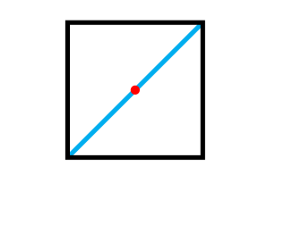
Figure 6: The figure represents the extraordinary canonical forms associated with the boundary of the cube, Eq. (9.8) with $\kappa\neq 0$. The extraordinary separable states are represented by the red dot and the extraordinary entangled states by the cyan diagonal. The square represents extraordinary witnesses. The extraordinary canonical forms are inequivalent to the ordinary ones (corresponding to $\kappa=0$) cohabiting the same set of points.

10 Measure and distillation of entanglement

The 4 dimensional description of the LSL equivalence classes of 2 qubits is faithful to the measure of entanglement. (This is not true for the 3 dimensional description in [28].) This allows us to give a geometric interpretation of the notion of concurrence and optimize distillation.

10.1 Concurrence as the best evidence

A natural way to quantify entanglement is to measure the expected values of entanglement witnesses [29]. Given an entangled state $\rho$, the entanglement evidence given by the expectation of the optimal witness is

$$\textsf{C}(\rho) = -\inf_{W}2\,Tr(W\rho)=-8\,\inf_{{\sf w}}{\sf w}^{\mu}{\sf r}_{\mu}$$ (10.1)

$$= 2(-{\sf r}_{0}+|{\sf r}_{1}|+|{\sf r}_{2}|+|{\sf r}_{3}|)$$

The set $W$ in this definition is the set of witnesses with a normalized representer. For a separable state the r.h.s. of Eq. (10.1) is clearly negative and one simply defines $\textsf{C}(\rho)=0$. It is clear from its definition that $\textsf{C}(\rho)$ is a positive quantity if and only if the state $\rho$ is entangled. It can be interpreted geometrically as the distance from the octahedral cone of separable state and it vanishes, of course, on its faces. It is clearly an LSL invariant. This is illustrated in Fig. 7.

Choosing the representative of the state $\sf r$ in the fundamental domain, Eq. (9.7), we have

$$\textsf{C}(\rho) = 2(-{\sf r}_{0}+{\sf r}_{1}+{\sf r}_{2}+|{\sf r}_{3}|)_{+}$$

$$= 2(-{\sf r}_{0}+{\sf r}_{1}+{\sf r}_{2}-{\sf r}_{3})_{+}$$

$$= (\rho_{0}-\rho_{1}-\rho_{2}-\rho_{3})_{+}$$

where we use the notation

$$(x)_{+}=\left\{\begin{array}[]{ll}x,&\hbox{$x>0$;}\\ 0,&\hbox{otherwise.}\\ \end{array}\right.$$ (10.3)

In the second line of (10.1) we have used the fact that for any state $({\sf r}_{0}-{\sf r}_{1}-{\sf r}_{2}-{\sf r}_{3})=\rho_{3}>0$. The third line is the standard definition of concurrence [51].

10.2 Entanglement distillation

Entanglement is easy to destroy (by mixing) and impossible to increase by local operations. However, one can sometimes distill entanglement by local operations at the price of loosing some of the qubits [48]. We have seen in section 5.2 that one can distill Bell states from a pure mixed state with finite success probability. Here we shall establish a bound on the maximal entanglement one can distill from a single mixed state with finite probability. This should be distinguished from the more common distillation protocols, say [6], which rely on operations on multiple identical copies of the state. Single copy distillation actually appears as a preliminary step in more general multi-copy protocols [21].

Geometrically, the results are summarized in Fig. 7. More precisely

Theorem 10.1.

Let $\sf{C}(\rho)>0$ be the concurrence of the state $\rho$ and let $M$ be the LSL transformation that takes it into its canonical diagonal form. The optimally distilled state is

$$\rho_{f}=\frac{M\rho M^{\dagger}}{Tr(M\rho M^{\dagger})}$$ (10.4)

Its concurrence is

$$\sf{C}(\rho_{f})=\frac{\sf{C}(\rho)}{4{\sf r}_{0}(\rho)}=\frac{(\rho_{0}-\rho_{1}-\rho_{2}-\rho_{3})_{+}}{\rho_{0}+\rho_{1}+\rho_{2}+\rho_{3}}\geq\sf{C}(\rho)$$ (10.5)

and the distillation succeeds with probability $p(\rho)$

$$p(\rho)\sf{C}(\rho_{f})=\frac{\textsf{C}(\rho)}{\|M\|^{2}}\leq\textsf{C}(\rho)$$ (10.6)

Proof: By the LSL invariance of the concurrence $\textsf{C}(\rho^{M})=\textsf{C}(\rho)$. It is then clear from Eq. (10.4) that the concurrence of the renormalized filtered state $\rho_{f}$ is maximal exactly when $Tr(M\rho M^{\dagger})$ takes its minimal value $4{\sf r}_{0}(\rho)$, which occurs precisely when $\rho_{f}$ is self dual, by theorem 7.2. This establishes the optimal concurrence. The probability that distillation succeeds is computed as in Eq.(5.5). $\square$

Since $0<4{\sf r}_{0}\leq 1$ the entanglement always increases, except for the states with $4{\sf r}_{0}=1$. These are the states represented by the cap of the cone, i.e entanglement can not be distilled when the subsystems are fully mixed. On the other hand, pure states have $\rho_{j}=0$ and thus can be filtered to be maximally entangled.

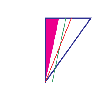
Figure 7: The pink triangle is the cone of separable states. The green line is a line of constant concurrence. Concurrence increases towards the right. The enclosing blue triangle illustrates the cone of states. States represented by the intersection of the red and green lines can be filtered along the red line. All states can be filtered to have zero entanglement, but in general not to maximal entanglement.

11 The Peres-Horodecki separability test

The geometric description of the world of 2 qubits allows for a simple proof, essentially by inspection, of the “only if” part of theorem 3.2. A similar elementary geometric proof is given in [28].

By Eq. (3.6), partial transposition acts on operators in canonical form as the reflection about the $\sigma_{3}^{\otimes 2}$ axis. States satisfying the Peres test are then those belonging to the intersection of the tetrahedron with its reflection which is precisely the octahedron of separable states. This shows that a state that satisfies the Peres test must be separable.

The original proof of this fact [23] is algebraic in character, more powerful, and not completely elementary. An elegant version of it also follows from the Choi-Jamiolwosky isomorphism [12] and an alternate simple proof is given in [48].

Acknowledgment

We thank G. Bisker, M. Goldstein, and N. Lindner for discussions, Lajos Diosi and Eli Meirom for comments and criticism of an earlier draft on the manuscript and P. Horodecki for pointing out ref. [53]. We acknowledge support by the Israel Science Foundation and the fund for promotion of research at the Technion.

Appendix A The existence of a minimizer

To extend theorem 7.1 to the boundary one needs a stronger version of lemma 7.4:

Lemma A.1.

• Suppose $\rho$ and $W$ both lie in the interior of the cone of potential witnesses, i.e. satisfying a strict inequality in (8.1). Then, the function $Tr\left(\rho W^{M}\right)$ diverges to $+\infty$ as either $M_{A}\in SL(2,\mathbb{C})$ or $M_{B}\in SL(2,\mathbb{C})$ go to infinity. In particular, it has a finite minimizer.

• For any $\rho$ and $W$ in the cone of potential witnesses, (boundary included) the function $Tr\left(\rho W^{M}\right)$ has a finite lower bound.

• Suppose $\rho$ satisfies a strict inequality (8.1) while $W$ satisfies only a weak one. In this case the infimum may be reached for infinite $M$. However, the corresponding $W^{M}$ is still guaranteed to have a finite limit.

Proof: Writing the potential witnesses $A,B$ in terms of their associated Lorentz tensors one has $\mbox{$\frac{1}{4}$}Tr(A{B}^{M_{1}\otimes M_{2}})=({\sf A})^{\mu\nu}(\Lambda_{1}{\sf B}\Lambda_{2})_{\mu\nu}$. We would like to consider the behavior of this expression when the Lorentz transformations $\Lambda_{1},\Lambda_{2}\in SO_{+}(1,3)$ involve large boosts.

Any Lorentz transformation $\Lambda$ may be written as a combination of a boost of some rapidity $t$ and a rotation. It is then always possible to express $\Lambda$ as

$$\Lambda(t)=e^{t}\Lambda_{+}+e^{-t}\Lambda_{-}+\Lambda_{0}.$$

Moreover one may write $\Lambda_{+}=v_{+}\otimes u_{+},\Lambda_{-}=v_{-}\otimes u_{-},\Lambda_{0}=v_{0,[1]}\otimes u_{0,[1]}+v_{0,[2]}\otimes u_{0,[2]}$ where $\{u_{+},u_{-},u_{0,[1]},u_{0,[2]}\},\{v_{+},v_{-},v_{0,[1]},v_{0,[2]}\}$ are two “light cone” bases of space-time. In the following it will be convenient not to bother with the distinction between the two spatial vectors $u_{0,[1]},u_{0,[2]}$ (or $v_{0,[1]},v_{0,[2]}$) and we will usually refer to both of them as $u_{0}$ (or $v_{0}$) with the extra index implicit.

Expressing the two Lorentz transformations as above one may write

$$({\sf A})^{\mu\nu}(\Lambda_{1}{\sf B}\Lambda_{2})_{\mu\nu}=\sum_{\alpha,\beta}e^{\alpha t_{1}}e^{\beta t_{2}}\left(u_{\beta}^{(2)}\cdot{\sf A}v_{\alpha}^{(1)}\right)\left(u_{\alpha}^{(1)}\cdot{\sf B}\ v_{\beta}^{(2)}\right)$$

where $\alpha,\beta$ run over the three values $+,-,0$. Using obvious notations this may be written more shortly as $\sum_{\alpha,\beta}e^{\alpha t_{1}}e^{\beta t_{2}}A_{\beta\alpha}B_{\alpha\beta}$

Consider the case where both $t_{1},t_{2}\rightarrow\infty$. It is clear that in this limit our function is dominated by the $(\alpha,\beta)=(+,+)$ term: $f\simeq e^{t_{1}+t_{2}}A_{++}B_{++}$. Relation (8.1) tells us that $A_{++},B_{++}\geq 0$. In particular if $A,B$ are strictly in the interior of the cone then they satisfy strict inequality and hence $f\rightarrow+\infty$ proving part 1 of the lemma.

The second part of the lemma concerns the case where the leading asymptotic term $A_{++}B_{++}$ vanishes. Suppose this is due to $B_{++}=0$, this means $Bv_{+}^{(2)}\perp u_{+}^{(1)}$. But we know that $Bv_{+}^{(2)}$ must be in the forward lightcone. This is consistent with $Bv_{+}^{(2)}\perp u_{+}^{(1)}$ only if $Bv_{+}^{(2)}\propto u_{+}^{(1)}$, which in turn implies $u_{0}^{(1)}\cdot Bv_{+}^{(2)}=0$, i.e. $B_{0+}=0$. Similarly, one also has $B_{+0}=0$. We conclude that contributions of the three terms $(\alpha,\beta)=(+,+),(+,0),(0,+)$ vanish. Since the $(\alpha,\beta)=(+,-),(-,+)$ terms are non-negative while $(\alpha,\beta)=(0,0),(0,-),(-,0),(-,-)$ are bounded, one concludes that $f$ has a lower bound proving part 2 of the lemma.

To check how $\Lambda_{1}{\sf B}\Lambda_{2}$ corresponding to $B^{M}$ behave as $t_{1},t_{2}\rightarrow\infty$, it is enough to consider its components with respect to the ($t$-independent!) $\{u\},\{v\}$ bases, which are just $e^{\alpha t_{1}}e^{\beta t_{2}}B_{\alpha\beta}$. We already saw that for the infimum to occur at infinite $t$ one must have $B_{++}=B_{+0}=B_{0+}=0$. Thus the only terms with the potential to diverge are $B_{+-},B_{-+}$. These however are strictly non-negative terms and so their divergence would imply $Tr(A{B}^{M})\rightarrow+\infty$ (assuming $A_{+-},A_{-+}\neq 0$ for a strict witness $A$). This phenomenon clearly cannot occour at an infimum of $Tr(A{B}^{M})$ and thus we conclude that all components of $B^{M}$ must have a finite limit proving part 3 of the lemma.

For completeness one should also remark on the case where only one of the $t_{i}$’s diverges, say $t_{2}\rightarrow\infty$. This may be dealt with similarly to the above by considering the function $\Lambda\mapsto Tr(C\Lambda)$ with $C\equiv A\Lambda_{1}B$ constant. $\square$

Appendix B Proof of Classification theorem 8.2

Since the matrix of Lorentz components ${\sf W}$ maps the forward light-cone into itself, so do ${\sf W}^{\star}$ and ${\sf W}^{\star}{\sf W}$. The projective space associated with the forward lightcone (i.e. causal 4-vectors modulo normalization) is geometrically a closed three dimensional ball. Since the closed unit ball is a fixed point domain, [44], the map ${\sf W}^{\star}{\sf W}$ must have a fixed point. Let $u_{0}$ be the associated direction, and $v_{0}$ the corresponding direction for ${\sf W}{\sf W}^{\star}$, i.e.

$${\sf W}^{\star}{\sf W}\,u_{0}=\lambda\,u_{0}\,,\quad{\sf W}{\sf W}^{\star}\,v_{0}=\lambda^{\prime}\,v_{0}.$$ (B.1)

In fact ${\sf W}\,u_{0}$ can be taken as a multiple of $v_{0}$. It then follows $\lambda^{\prime}=\lambda$ and ${\sf W}\,v_{0}$ is a multiple of $u_{0}$,

$${\sf W}\,u_{0}=\sqrt{\lambda}\,v_{0}\,,\quad{\sf W}^{\star}\,v_{0}=\sqrt{\lambda}\,u_{0}$$ (B.2)

There are now 4 cases. The ordinary case is when $u_{0}$ and $v_{0}$ are time-like. The three extraordinary cases correspond to the situations when either $u_{0}$ or $v_{0}$, or both are light-like.

B.1 The ordinary case

The ordinary case distinguishes two Lorentz frames, one whose time axis coincides with $u_{0}$ and another whose time axis coincides with $v_{0}$. Since both vectors are time-like they can be normalized $u_{0}\cdot u_{0}=v_{0}\cdot v_{0}=1$. Let $u_{j}$ and $v_{j}$ span the space-like directions corresponding to $u_{0}$ and $v_{0}$ respectively. Since

$$v_{j}\cdot{\sf W}\,u_{0}=\sqrt{\lambda}\,v_{j}\cdot v_{0}=0,\quad v_{0}\cdot{\sf W}\,u_{j}=\sqrt{\lambda}\,u_{0}\cdot u_{j}=0$$ (B.3)

the pair of Lorentz frames bring ${\sf W}$ to a form where ${\sf W}_{0j}={\sf W}_{j0}=0$. The remaining $3\times 3$ spatial block can be diagonalized by a pair of spatial rotations, leading to the form (8.10). The condition ${\sf w}_{0}\geq|{\sf w}_{j}|$ follows from the requirement that ${\sf W}$ maps the forward light-cone into itself.

B.2 The second and third extraordinary case

Consider the case where at least one of causal eigenvectors $u_{0},v_{0}$ is null.

Suppose $u_{0}^{2}=1$ but $v_{0}^{2}=0$. The assumption that $\sf{W}\sf{W}^{\star}$ does not have time-like eigenvectors then implies that ${\sf W}u_{0}$ must be null (or zero). This in turn implies $0=({\sf W}u_{0})^{2}=u_{0}\cdot{\sf W}^{\star}{\sf W}u_{0}=\lambda u_{0}^{2}=\lambda$. Similarly $u_{0}^{2}=0,v_{0}^{2}=1$ also implies $\lambda=0$.

Assume now that $\lambda=0$ for whatever reason. ${\sf W}^{\star}{\sf W}u_{0}=0$ then implies either ${\sf W}u_{0}=0$ or ${\sf W}u_{0}\propto v_{0},\,{\sf W}^{\star}v_{0}=0$. Let us concentrate on one of these possibilities, say ${\sf W}^{\star}v_{0}=0$. It then follows $u\cdot{\sf W}^{\star}v_{0}=0\;\forall u$, i.e. $v_{0}\cdot{\sf W}u=0\;\forall u$. This relation should hold in particular for any causal vector $u$, in which case we know that ${\sf W}u$ is also causal. However it is well known that two nonzero vectors both inside the light cone can be orthogonal only if they are a pair of parallel null vectors. We conclude thus that ${\sf W}u\propto v_{0}$. This must hold for any causal $u$ and hence by linearity for all $u$’s. It follows $\sf{W}$ is a rank one matrix of the form $v_{0}\otimes u$ for some $u$ which is easily identified with $u_{0}$. This means that $\sf W$ is of the form (8.15). The case ${\sf W}u_{0}=0$ similarly leads to Eq. (8.14)

B.3 The first extraordinary case

The case of $u_{0}^{2}=v_{0}^{2}=0$ (and $\lambda\neq 0$) is the hardest one to analyze.

Consider first the self dual case ${\sf A}={\sf W^{\star}W}$ having null eigenvector $u_{0}$. One then has a Jordan block spanned by $\{u_{0},u_{1},...u_{k}\}$ such that $Au_{i}=\lambda u_{i}+u_{i-1}$ (here $u_{-1}\equiv 0$). It should be noted that there is always some freedom in the choice of the $u_{i}$’s. Specifically we may add to $u_{i}$ any multiple of $u_{j},\,j<i$. Smart choices may help simplifications. We shall make use of the identity $u_{i}\cdot u_{j}=u_{i+1}\cdot u_{j-1}$ which follows from the relation $u_{i}\cdot Au_{j}=u_{j}\cdot Au_{i}$.

• If $k=1$ then we must have $u_{1}\cdot u_{0}\neq 0$, for otherwise it cannot span anything outside $u_{0}^{\perp}$. (Other eigenspaces must of course be orthogonal to $u_{0}$.) Taking advantage of our freedom to add to $u_{1}$ any multiple of $u_{0}$ we may then assume $u_{1}^{2}=0$. Identifying $u_{0},u_{1}$ with standard light like vectors $(1,\pm 1,0,0)$ we then find $A$ takes the form (8.12) with ${\sf W}_{0}=\lambda,\kappa=\mbox{$\frac{1}{2}$}$, which is equivalent to ”type II” of [17].

• If $k=2$ then $u_{1}\cdot u_{0}=u_{2}\cdot u_{-1}=0$ imply that $u_{1}$ is space-like: $u_{1}^{2}<0$. We then also have $u_{2}\cdot u_{0}=u_{1}^{2}\neq 0$ from which it follows that by adding to $u_{1},u_{2}$ appropriate multiples of $u_{0}$ we may assume them to satisfy $u_{2}^{2}=u_{2}\cdot u_{1}=0$. It then follows that $Au_{2}=\lambda u_{2}+u_{1}$ maps a light-like vector to a spacelike one. This case is therefore not of our interest.

• The $k=3$ case may be disqualified on the same basis as $k=2$. However, stronger arguments exist. Note that $u_{1}^{2}=u_{3}\cdot u_{-1}=0$ contradicts $u_{1}\cdot u_{0}=u_{2}\cdot u_{-1}=0$ (unless $u_{1}\propto u_{0}$). Thus this case cannot arise even if one does not demand $A$ to be a potential witness.

We conclude that only the case $k=1$ is relevant. Given a non self dual $\sf W$ one may then define $u_{0},u_{1}$ and $v_{0},v_{1}$ as above corresponding to the self dual operators $A=\sf{W}^{\star}\sf{W}$ and $\sf{W}\sf{W}^{\star}$. Unless $\lambda=0$ one may pair $u_{0},v_{0}$ as in Eq. (B.2). Calculation then shows that ${\sf W}u_{1}-\sqrt{\lambda}v_{1}$ is an eigenvector of $\sf{W}\sf{W}^{\star}$ and hence proportional to $v_{0}$. One may then write:

$${\sf W}u_{0}=\sqrt{\lambda}v_{0},\;\;\;\;\;{\sf W}u_{1}=\sqrt{\lambda}v_{1}+\kappa v_{0}$$

Knowing how $\sf W$ acts on $u_{0}$ and $u_{1}$ essentially solves the classification problem and allows presenting it as in Eq. (8.12).

References

- [1] J. E. Avron, G. Bisker, and O. Kenneth. Visualizing two qubits. J. Math. Phys., 48:102107, 2007, quant-ph/0706.2466.
- [2] John S. Bell. Speakable and unspeakable in quantum mechanics. Cambridge U.P., 1993.
- [3] J.S. Bell. On the Einstein Podolsky Rosen paradox. Physics 1, 195, 1964.
- [4] Ingemar Bengtsson and Karol Zyczkowski. Geometry of Quantum States: An Introduction to Quantum Entanglement. Cambridge University Press, 2006.
- [5] Charles H. Bennett, Gilles Brassard, Claude Crépeau, Richard Jozsa, Asher Peres, and William K. Wootters. Teleporting an unknown quantum state via dual classical and Einstein-Podolsky-Rosen channels. em Phys. Rev. Lett., 70, (13); 1895–1899, 1993.
- [6] Charles H. Bennett, Herbert J. Bernstein, Sandu Popescu, and Benjamin Schumacher. Concentrating partial entanglement by local operations. Phys. Rev. A, 53(4):2046–2052, 1996.
- [7] Charles H. Bennett, Sandu Popescu, Daniel Rohrlich, John A. Smolin, and Ashish V. Thapliyal. Exact and asymptotic measures of multipartite pure-state entanglement. Phys. Rev. A, 63(1):012307, 2000.
- [8] Howard E. Brandt. Positive operator valued measure in quantum information processing. American Journal of Physics, 67(5):434–439, 1999.
- [9] Samuel L. Braunstein, A. Mann, and M. Revzen. Maximal violation of bell inequalities for mixed states. Phys. Rev. Lett., 68(22):3259–3261, 1992.
- [10] Hans J. Briegel and Robert Raussendorf. Persistent entanglement in arrays of interacting particles. Phys. Rev. Lett., 86(5):910–913, 2001.
- [11] Nicolas Brunner, Antonio Acín, Daniel Collins, Nicolas Gisin, and Valerio Scarani. Optical telecom networks as weak quantum measurements with postselection. Phys. Rev. Lett., 91(18):180402, 2003.
- [12] M. D. Choi. Completely positive linear maps on complex matrices. Lin. Alg. Appl., 10:285– 290, 1975.
- [13] John F. Clauser, Michael A. Horne, Abner Shimony, and Richard A. Holt. Proposed experiment to test local hidden-variable theories. Phys. Rev. Lett., 23(15):880–884, 1969.
- [14] E. Brian Davies Quantum theory of open systems Academic Press, 1976.
- [15] I. Gohberg, P. Lancaster, and L. Rodman. Matrices and Indefinite Scalar Products. Birkhauser Verlag, 1983.
- [16] Daniel M. Greenberger, Michael A. Horne, Abner Shimony, and Anton Zeilinger. Bell’s theorem without inequalities. American Journal of Physics, 58(12):1131–1143, 1990.
- [17] S. W. N. Hawking and G. F. R. Ellis. The large scale structure of space-time. Cambridge U.P., 1974.
- [18] P. Hayden, D. Leung, and A. Winter. Aspects of generic entanglement. Comm. Math. Phys., 265:95 117, 2007.
- [19] Alexander S. Holevo. Statistical structure of quantum theory. Springer, 2001.
- [20] M. E. Horodecki, P. Shor, and M. B. Ruskai. Entanglement breaking channels. Rev. Math. Phys, 15:629–641.
- [21] Michał Horodecki, Paweł Horodecki, and Ryszard Horodecki. Inseparable two spin- density matrices can be distilled to a singlet form. Phys. Rev. Lett., 78(4):574–577, 1997.
- [22] Michał Horodecki, Paweł Horodecki, and Ryszard Horodecki. Mixed-state entanglement and distillation: Is there a ‘bound’ entanglement in nature? Phys. Rev. Lett., 80(24):5239–5242, 1998.
- [23] Michał E. Horodecki, Paweł Horodecki, and Ryszard Horodecki. Separability of mixed states: necessary and sufficient conditions. Phys. Lett. A, 223(1):1–8, 1996.
- [24] Ryszard Horodecki and Michał Horodecki. Information-theoretic aspects of inseparability of mixed states. Phys. Rev. A, 54(3):1838–1843, 1996.
- [25] Horodecki, Ryszard and Horodecki, Paweł and Horodecki, Michał E. and Horodecki, Karl . Quantum entanglement. 2007, quant-ph/0702225.
- [26] Chris King and Mary Beth Ruskai. Minimal entropy of states. IEEE Trans. Info. Theory, 47:192—209, 1999, quant-ph/9911079.
- [27] Lev D. Landau and E. M. Lifshitz. The classical theory of fields. Butterworth Heinemann, 1973.
- [28] Jon Magne Leinaas, Jan Myrheim, and Eirik Ovrum. Geometrical aspects of entanglement. Phys. Rev. A, 74(1):012313, 2006.
- [29] M. Lewenstein, B. Kraus, J. I. Cirac, and P. Horodecki. Optimization of entanglement witnesses. Phys. Rev. A, 62(5):052310, 2000.
- [30] David N. Mermin. Boojoums all the way through. Cambridge U.P., 1990.
- [31] David N. Mermin. Some curious facts about quantum factoring. Physics Today, 60(10):10–11, 2007.
- [32] R emy Mosseri and Rossen Dandoloff. Geometry of entangled states, bloch spheres and hopf fibrations. J. Phys. A, 43(5):10243 10252, 2001.
- [33] Gisin N. Hidden quantum nonlocality revealed by local filters. Phys. Lett. A, 210:151–156(6), 8 1996.
- [34] Michael A. Nielsen and Isaac L. Chuang. Quantum Computation and Quanum Information. Cambridge U.P., 2000.
- [35] Asher Peres. Quantum Theory: Concepts and Methods. Springer, 1995.
- [36] Asher Peres. Separability criterion for density matrices. Phys. Rev. Lett., 77(8):1413–1415, 1996.
- [37] Michael E. Peskin and Daniel E. Schroeder. An introduction to quantum field theory. Perseus Books, 1995.
- [38] Martin B Plenio and Vlatko Vedral. Teleportation, entanglement and thermodynamics in the quantum world. Contemporary Physics, 39(6):431, 1998.
- [39] Martin B. Plenio and Shashank Virmani An introduction to entanglement measures. arXiv:quant-ph/0504163v3, 2006
- [40] Tyrrell R. Rockafellar. Convex Analysis. Princeton University Press, 1970.
- [41] Mary Beth Ruskai. Qubit entanglement breaking channels. Rev. Math. Phys, 15:643–662, 2003, quant-ph/0302032v3.
- [42] Mary Beth Ruskai, Stanislaw Szarek, and Elisabeth Werner. An analysis of completely-positive trace-preserving maps on 2x2 matrices. 2001, quant-ph/0101003v2.
- [43] Marlan O. Scully and M. Suhail Zubairy. Quantum Optics. Cambridge University Press, 1977.
- [44] D. R. Smart. Fixed point theorems. Cambridge University Press, 1974.
- [45] Constantino Tsallis, Seth Lloyd, and Michel Baranger. Peres criterion for separability through nonextensive entropy. Phys. Rev. A, 63(4):042104, 2001.
- [46] B.M Tsirelson. Some results and problems on quantum bell-type inequalities. 8:329–345, 1993.
- [47] Frank Verstraete, Jeroen Dehaene, and Bart De Moor. Lorentz singular-value decomposition and its applications to pure states of three qubits. Phys. Rev. A, 65(3):032308, 2002.
- [48] Frank Verstraete, Jeroen Dehaene, and Bart DeMoor. Local filtering operations on two qubits. Phys. Rev. A, 64(1):010101, 2001.
- [49] G. Vidal and R. F. Werner. Computable measure of entanglement. Phys. Rev. A, 65(3):032314, 2002.
- [50] R.F. Werner. Quantum states with Einstein-Rosen-Podolsky correlations admitting a hidden-variable model. Phys. Rev. A, 40:4277–4281, 1989.
- [51] William K. Wootters. Entanglement of formation of an arbitrary state of two qubits. Phys. Rev. Lett., 80(10):2245–2248, 1998.
- [52] William K. Wootters. Entanglement of formation and concurrence. Quantum Information and Computation, 1(1):27–44, 2001.
- [53] Marek Zcachor. Teleportation seen from space-time: On two-spinor aspects of quantum information processing. arXiv:0803.3289v4, 2008.
- [54] Karol Zyczkowski and Ingemar Bengtsson. On duality between quantum maps and quantum states. Open Systems and Information Dynamics, 11(1):3–42.
- [55] Karol Zyczkowski and Ingemar Bengtsson. An introduction to quantum entanglement: a geometric approach, 2006.