Abstract

In the $k_{T}$-factorization for exclusive processes, the nontrivial $k_{T}$-dependence of perturbative coefficients, or hard parts, is obtained by taking off-shell partons. This brings up the question of whether the $k_{T}$-factorization is gauge invariant. We study the $k_{T}$-factorization for the case $\pi\gamma^{*}\rightarrow\gamma$ at one-loop in a general covariant gauge. Our results show that the hard part contains a light-cone singularity that is absent in the Feynman gauge, which indicates that the $k_{T}$-factorization is not gauge invariant. These divergent contributions come from the $k_{T}$-dependent wave function of $\pi$ and are not related to a special process. Because of this fact the $k_{T}$-factorization for any process is not gauge invariant and is violated. Our study also indicates that the $k_{T}$-factorization used widely for exclusive $B$-decays is not gauge invariant and is violated.

When large momentum transfers happen in exclusive processes, one can employ perturbation theory of QCD thanks to its asymptotic freedom. However, a pre-condition for using the perturbation theory is to consistently factorize perturbative effects from nonperturbative effects in amplitudes of exclusive processes. It has been proposed long time ago that the factorization of amplitudes can be made by expanding amplitudes in the inverse of the large momentum transfers[1, 2]. The expansion corresponds to the twist expansion of QCD operators characterizing nonperturbative effects. The leading term can be factorized as a convolution of a hard part and light-cone wave functions of hadrons. The light-cone wave functions are defined with QCD operators, and the hard part describes hard scattering of partons at short distances. In this factorization the transverse momenta of partons in parent hadrons are also expanded in the hard scattering part, and they are neglected in the leading twist. Because of this, the light-cone wave functions depend only on the longitudinal momentum fractions carried by partons, not on transverse momenta of partons. This is the so-called collinear factorization.

Later, $k_{T}$-factorization was proposed[3], in which the transverse momenta, neglected in collinear factorization, are taken into account. The effects of the transverse-momentum of partons in hadrons are described by wave functions and those in the hard scattering are described by a hard part which depends on $k_{T}$. The $k_{T}$-factorization has been widely used in exclusive $B$-decays, a partial list of references can be found in [4, 5], where it is often called the perturbative QCD(pQCD) approach. The factorization has some advantages in that it includes some higher twist effects and re-sums the Sudakov logarithms (see e.g., [4, 5] and references therein). However, the factorization has not been examined extensively as the collinear factorization. It is possible that the $k_{T}$-factorization is violated. It should be noted that the nontrivial $k_{T}$-dependence of the hard part at the tree-level is obtained with off-shell partons entering hard scattering. This brings up the question if the hard part is gauge invariant. Recently, the $k_{T}$-factorization has been studied at the one-loop level for $\pi^{0}+\gamma^{*}\rightarrow\gamma$[6]. The study is done with the Feynman gauge and it is claimed that the hard part with the off-shell parton is gauge invariant[6]. In this letter we examine the $k_{T}$-factorization of the process in a general covariant gauge. It turns out that the hard part obtained with off-shell partons is not gauge invariant. Moreover, the hard part in the general covariant gauge contains special singularities called light-cone singularities, although the hard part in the Feynman gauge is finite at one-loop according to ref. [6]. The contributions of the singularities come from the wave function. This indicates that the $k_{T}$-factorization is not gauge invariant and is, in general, violated.

We consider the process $\pi^{0}(P)+\gamma^{*}\rightarrow\gamma(p)$. We will use the light-cone coordinate system, in which a vector $a^{\mu}$ is expressed as $a^{\mu}=(a^{+},a^{-},\vec{a}_{\perp})=((a^{0}+a^{3})/\sqrt{2},(a^{0}-a^{3})/\sqrt{2},a^{1},a^{2})$ and $a_{\perp}^{2}=(a^{1})^{2}+(a^{2})^{2}$. We take a frame in which $\pi^{0}$ has the momentum $P^{\mu}=(P^{+},P^{-},0,0)$ with $P^{+}\gg P^{-}$ and the outgoing photon has $p^{\mu}=(0,p^{-},0,0)$. The relevant form factor and its $k_{T}$ factorization[6] are:

$$\langle\gamma(p,\epsilon^{*})|\bar{q}\gamma^{\mu}q|\pi^{0}(P)\rangle=i\varepsilon^{\mu\nu\rho\sigma}\epsilon^{*}_{\nu}P_{\rho}p_{\sigma}F(Q^{2}),\ \ \ Q^{2}=-(P-p)^{2},$$

$$F(Q^{2})=\int dxd^{2}k_{T}\phi(x,k_{T})H(x,k_{T})\left(1+{\mathcal{O}}(Q^{-2})\right),$$ (1)

where $\phi$ is the wave function defined below, and $H$ is the hard part. If the $k_{T}$-factorization holds, the hard part $H$ can be calculated safely with perturbative QCD. We introduce a vector $u^{\mu}=(u^{+},u^{-},0,0)$ such that the wave function for $\pi^{0}$ can be defined in the limit $u^{+}<<u^{-}$[6, 7, 8]:

$$\phi(x,k_{T},\zeta,\mu) = \ \int\frac{dz^{-}}{2\pi}\frac{d^{2}z_{\perp}}{(2\pi)^{2}}e^{ik^{+}z^{-}-i\vec{z}_{\perp}\cdot\vec{k}_{T}}\langle 0|\bar{q}(0)L_{u}^{\dagger}(\infty,0)\gamma^{+}\gamma_{5}L_{u}(\infty,z)q(z)|\pi^{0}(P)\rangle|_{z^{+}=0},$$

$$k^{+} = xP^{+},\ \ \ \ \ \zeta^{2}=\frac{2u^{-}(P^{+})^{2}}{u^{+}}\approx\frac{4(u\cdot P)^{2}}{u^{2}},$$ (2)

where $q(x)$ is the light-quark field. $L_{u}$ is the gauge link in the direction $u$:

$$L_{u}(\infty,z)=P\exp\left(-ig_{s}\int_{0}^{\infty}d\lambda u\cdot G(\lambda u+z)\right).$$ (3)

The hard part $H$ is obtained by replacing the hadron state with a parton state. With the parton state one can calculate the wave function and the form factor, and hence can determine the hard part. We replace $\pi^{0}$ with the partonic state $|q(k_{1}),\bar{q}(k_{2})\rangle$ with the momenta given as

$$k_{1}^{\mu}=(k_{1}^{+},k_{1}^{-},\vec{k}_{1\perp}),\ \ \ \ k_{2}^{\mu}=(k_{2}^{+},k_{2}^{-},-\vec{k}_{1\perp}),\ \ \ \ \ \ k_{1}^{+}=x_{0}P^{+},\ \ \ \ k_{2}^{+}=(1-x_{0})P^{+}=\bar{x}_{0}P^{+}.$$ (4)

If we take the partons on-shell, we have the wave function at tree-level:

$$\phi^{(0)}(x,k_{T},\zeta)=\delta(x-x_{0})\delta^{2}(\vec{k}_{T}-\vec{k}_{1\perp})\bar{v}(k_{2})\gamma^{+}\gamma_{5}u(k_{1})/P^{+}.$$ (5)

For the same parton state, the form factor receives contributions from the diagrams in Fig.1. Through a simple calculation one can determine the hard part at tree-level as:

$$Q^{2}H^{(0)}=\frac{1}{x}+\frac{1}{\bar{x}},\ \ \ \ \bar{x}=1-x.$$ (6)

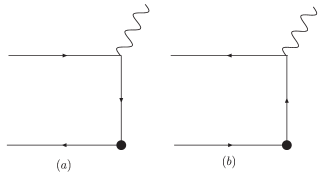
Figure 1: The tree-level diagrams of the form factor.

With the on-shell parton, one obtains the hard part which does not depend on $k_{T}$, although the partons entering the hard scattering have nonzero transverse momenta. The dependence can be obtained if one takes the parton state with off-shell partons. Following the $k_{T}$-factorization illustrated in ref. [6], we take partons off-shell with the momenta:

$$k_{1}^{\mu}=(k_{1}^{+},0,\vec{k}_{1\perp}),\ \ \ \ k_{2}^{\mu}=(k_{2}^{+},0,-\vec{k}_{1\perp}),$$ (7)

and replace the product of spinors by:

$$u(k_{1})\bar{v}(k_{2})\rightarrow\gamma_{5}\gamma^{-},$$ (8)

to pick up the leading twist contributions. With the off-shell partons one indeed gets the hard part depending on $k_{T}$:

$$H^{(0)}=\frac{1}{xQ^{2}+k^{2}_{T}}+\frac{1}{\bar{x}Q^{2}+k^{2}_{T}},$$ (9)

where the first and the second term come from Fig. 1a and Fig. 1b, respectively.

In general, the quantities calculated with off-shell partons are not gauge invariant. The one-loop hard part extracted from

$$H^{(1)}\otimes\phi^{(0)}=F^{(1)}-H^{(0)}\otimes\phi^{(1)}$$ (10)

can not be expected to be gauge invariant. In ref. [6], $H^{(1)}$ is calculated in the Feynman gauge and it is claimed that $H^{(1)}$ is gauge invariant. In this letter we will study $H^{(1)}$ in a covariant gauge. Because of the symmetry of charge-conjugation we only need to consider the one-loop correction of Fig.1a and its factorization.

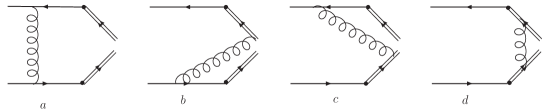
Figure 2: The one-loop diagrams of the wave function.

We take a general covariant gauge. In the gauge the gluon propagator is given by:

$$\frac{-i}{q^{2}+i\varepsilon}\left(g^{\mu\nu}-\alpha\frac{q^{\mu}q^{\nu}}{q^{2}+i\varepsilon}\right)$$ (11)

where $\alpha$ is the gauge parameter. The Feynman gauge is obtained by taking $\alpha=0$. At one-loop the wave function receives contributions from diagrams given in Fig. 2 and Fig. 3. The contributions from Fig. 3 are proportional to the tree-level result. The contribution from Fig. 2b reads:

$$\phi|_{2b} = \int\frac{d^{4}q}{(2\pi)^{4}}\bar{v}(k_{2})\gamma^{+}\gamma^{5}\left(ig_{s}u^{\mu}T^{a}\right)\frac{-i}{u\cdot q-i\varepsilon}\frac{i\gamma\cdot(k_{1}-q)}{(k_{1}-q)^{2}+i\varepsilon}\left(-ig_{s}\gamma^{\nu}T^{a}\right)u(k_{1})$$ (12)

$$\cdot\frac{-i}{q^{2}+i\varepsilon}\left(g^{\mu\nu}-\alpha\frac{q^{\mu}q^{\nu}}{q^{2}+i\varepsilon}\right)\delta(k^{+}-(k_{1}-q)^{+})\delta^{2}(\vec{k}_{T}-(\vec{k}_{1}-\vec{q})_{\perp}),$$

where $q$ is the momentum carried by the gluon. At the one-loop level, the wave function will receive contributions which depend on $\alpha$. We denote these contributions as $\phi_{\alpha}$ and call them gauge parts. From Fig. 2b the gauge part is:

$$\phi_{\alpha}|_{2b}=i\frac{4\alpha g_{s}^{2}}{3(2\pi)^{3}}\int\frac{dq^{-}}{(2\pi)}\frac{{\rm Tr}\left[\gamma^{5}\gamma^{-}\gamma^{+}\gamma_{5}\gamma\cdot(k_{1}-q)\gamma\cdot q\right]}{((k_{1}-q)^{2}+i\varepsilon)(q^{2}+i\varepsilon)^{2}}=i\frac{16\alpha g_{s}^{2}}{(2\pi)^{3}}\int\frac{dq^{-}}{(2\pi)}\frac{\left[2k_{1}^{+}q^{-}-\vec{k}_{1\perp}\cdot\vec{q}_{\perp}-q^{2}\right]}{((k_{1}-q)^{2}+i\varepsilon)(q^{2}+i\varepsilon)^{2}}.$$ (13)

The $q^{-}$-integral can easily be performed by taking a contour. Then one can calculate the convolution which contributes to $H^{(1)}$:

$$\phi_{\alpha}|_{2b}\otimes H^{(0)}=\int_{0}^{1}dx\int d^{2}k_{T}\frac{1}{xQ^{2}+k_{T}^{2}}\phi_{\alpha}|_{2b}.$$ (14)

This integral is divergent. The divergence comes from the region of $x\rightarrow x_{0}$ and $\vec{k}_{T}\rightarrow\vec{k}_{1\perp}$. With $q^{+}=k_{1}^{+}-k^{+}$ and $\vec{q}_{\perp}=\vec{k}_{1\perp}-\vec{k}_{T}$ this region corresponds to the region where the gluon momentum $q$ scales as $q^{\mu}=Q(\delta^{2},{\mathcal{O}}(1),\delta,\delta)$ with $\delta$ approaching to zero. Here $Q$ is a scale. In that region $q^{2}$ scales as $\delta^{2}$ and goes to zero. This results in a divergence that comes from the first term in Eq.(13). Since $q^{-}$ is much larger than $q^{+}$ and $|\vec{q}_{\perp}|$, the divergence is a light-cone divergence, and the corresponding singularity can be called as light-cone singularity. It should be emphasized that the singularity is not an infrared(I.R.) singularity. By isolating the divergence one can find that the divergent part of the convolution is proportional to the divergent integral:

$$\int_{0}^{x_{0}}dx\frac{1}{x_{0}-x}=\int_{0}^{k_{1}^{+}}\frac{dq^{+}}{q^{+}}.$$ (15)

The singularity comes from the end-point at $q^{+}=0$. The restriction of $q^{+}<k_{1}^{+}$ is from the definition of the wave function with $k^{+}=xP^{+}=k_{1}^{+}-q^{+}>0$. Later, we will discuss the appearance of the singularity in more detail.

The singularity comes from the gauge part of the gluon propagator. One can introduce a gluon mass $\lambda_{L}$ to regularize the light-cone singularity. With the mass $\lambda_{L}$ the gluon propagator reads[10]:

$$\frac{-i}{q^{2}-\lambda_{L}^{2}+i\varepsilon}\left[g^{\mu\nu}-\alpha\frac{q^{\mu}q^{\nu}}{q^{2}-(1-\alpha)\lambda_{L}^{2}+i\varepsilon}\right].\\$$

the divergent part of $\phi_{\alpha}|_{2b}$ can be found as:

$$\phi_{\alpha}|_{2b} = -\frac{4\alpha\alpha_{s}}{\pi^{2}}\theta(x_{0}-x)\frac{k^{2}_{1\perp}}{k_{1}^{+}\left[q^{2}_{\perp}+y_{q}k^{2}_{1\perp}+\lambda_{L}^{2}\right]\left[q^{2}_{\perp}+y_{q}k^{2}_{1\perp}+\bar{\alpha}\lambda_{L}^{2}\right]}+{\rm finite\ terms},$$

$$\bar{\alpha} = 1-\alpha,\ \ \ \ \ y_{q}=\frac{q^{+}}{k_{1}^{+}}=\frac{x_{0}-x}{x_{0}}.$$ (16)

With the gluon mass we obtain the divergent part of the convolution:

$$\phi_{\alpha}|_{2b}\otimes H^{(0)}=\frac{4\alpha\alpha_{s}}{P^{+}\pi}\frac{\ln\lambda_{L}^{2}}{x_{0}Q^{2}+k_{1\perp}^{2}}+{\rm finite\ terms}.$$ (17)

It should be pointed out that the contour integral of $q^{-}$ may cause some problems at first glance, because the integral becomes singular in the region of $q^{+}\sim 0$. However, once the singularity is regularized as in the above, the contour integral is well-defined. One can also use dimensional regularization to regularize the singularity as the pole of $d-4$.

In the convolution of Fig. 2c and Fig. 2a there are similar singularities. Working out the singular contributions we have for the divergent parts:

$$\phi_{\alpha}|_{2c}\otimes H^{(0)} = \frac{4\alpha\alpha_{s}}{P^{+}\pi}\frac{\ln\lambda_{L}^{2}}{x_{0}Q^{2}+k_{1\perp}^{2}}+{\rm finite\ terms},$$

$$\phi_{\alpha}|_{2a}\otimes H^{(0)} = -\frac{4\alpha\alpha_{s}}{P^{+}\pi}\frac{\ln\lambda_{L}^{2}}{x_{0}Q^{2}+k_{1\perp}^{2}}+{\rm finite\ terms},$$ (18)

We note that the sum of the three parts is still divergent. The gauge part of the contribution of Fig. 2d reads:

$$\phi_{\alpha}|_{2d}=i\alpha\frac{16g_{s}^{2}}{(2\pi)^{3}}\int\frac{dq^{-}}{2\pi}\frac{1}{(q^{2}+i\varepsilon)^{2}},$$ (19)

where $q$ is the momentum carried by the gluon. When convoluted with a test function, one can see that this part only contributes in the region $q^{+}\sim 0$. For $q^{+}\neq 0$ one can perform the $q^{-}$-integral and get a result of zero. Therefore, we have:

$$\phi_{\alpha}|_{2d}=i\alpha\frac{16g_{s}^{2}}{(2\pi)^{3}}\delta(x-x_{0})\int_{k_{1}^{+}-P^{+}}^{k_{1}^{+}}\frac{dq^{+}}{P^{+}}\int\frac{dq^{-}}{2\pi}\frac{1}{(q^{2}+i\varepsilon)^{2}}.$$ (20)

Again it is divergent. The divergence is an I.R. singularity. We regularize the singularity with a finite gluon mass $\lambda_{I}$, and obtain the divergent part of the convolution:

$$\phi|_{2d}\otimes H^{(0)}=\frac{4\alpha_{s}}{P^{+}\pi}\left(2+\alpha\right)\frac{\ln\lambda_{I}^{2}}{x_{0}Q^{2}+k_{1\perp}^{2}}+{\rm finite\ terms},$$ (21)

where we also give the singular contribution which does not depend on $\alpha$. In the above convolutions the finite terms are also free from U.V. singularities, i.e., they do not depend on the renormalization scale $\mu$.

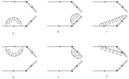
Figure 3: The one-loop diagrams of the wave function.

Now we turn to the contributions from Fig. 3. The contributions from Fig. 3a and Fig. 3d will not contribute to the hard part, because the same is also contained in the form factor. The contributions from other diagrams are:

$$\phi|_{3b} = \phi|_{3e}=-\frac{2\alpha_{s}}{\pi P^{+}}\delta(x-x_{0})\delta^{2}(\vec{k}_{T}-\vec{k}_{1\perp})\left[\left(2+\alpha\right)\ln\frac{\lambda^{2}_{I}}{\mu^{2}}-(1-\alpha)\ln(1-\alpha)-\alpha\right],$$

$$\phi|_{3c} = \phi|_{3f}=-\frac{4\alpha\alpha_{s}}{\pi P^{+}}\delta(x-x_{0})\delta^{2}(\vec{k}_{T}-\vec{k}_{1\perp})\left[\ln\frac{\mu^{2}}{k_{T}^{2}}+1\right]+\cdots,$$ (22)

where $\cdots$ denote contributions which do not depend on the gauge parameter $\alpha$. In the work of [6] the contributions from gluon exchange between gauge links, i.e., those from Fig. 2d, Fig. 3b and Fig. 3e, are simply neglected with the argument that these contributions or diagrams do not correspond to any part of the form factor. It is true that there are no corresponding parts in the form factor $F^{(1)}$, but the contributions from Fig. 2d, Fig. 3b and Fig. 3e exist by the definition of the wave function in Eq.(2). The existence of these contributions makes the wave function with on-shell partons gauge invariant. Without them this wave function is not gauge invariant. This can be shown with the general covariant gauge. We note that the sum of the contributions from the three diagrams to $H^{(1)}$ is free from I.R. singularities. However, the situation can become complicated beyond the one-loop level where the exchange of gluons between gauge links and the exchange of gluons between quark lines and gauge links can exist simultaneously, the cancellation of the I.R. singularities in this case can be problematic. A better way to deal the problem is to subtract these I.R. singularities by introducing a soft factor as shown in ref. [8, 9]. It should be noted that the contributions from Fig. 3 determine the $\mu$-dependence of the wave function. This $\mu$-dependence must be gauge invariant in order to make sure that the $\mu$-dependence of $H$ is gauge invariant, because the form factor does not depend on $\mu$. Neglecting the contributions from Fig. 3b and Fig. 3e, as in ref. [6], causes the $\mu$-dependence of the wave function to not be gauge invariant. This already implies that the hard part determined in ref. [6] is not gauge invariant.

It should be emphasized that the contributions from Fig. 3c and Fig. 3f do not have the light-cone singularity by our explicit calculation. For our conclusion presented in this letter, it is crucial to understand the absence of the singularity here. Part of the contribution of Fig. 3c is proportional to the integral

$$I^{\mu}=\int\frac{d^{4}q}{(2\pi)^{4}}\frac{q^{\mu}}{(q^{2}+i\varepsilon)^{2}((k_{1}-q)^{2}+i\varepsilon)}.$$ (23)

The light-cone singularity can appear in the component $I^{-}$ of $I^{\mu}$. From the Lorentz covariance one has $I^{\mu}\propto k_{1}^{\mu}$. This leads to $I^{-}=0$ because $k^{-}_{1}=0$. Therefore, the light-cone singularity does not exist in the contribution of Fig. 3c. The nonexistence can also be understood in another way, which is important for the later discussion of the form factor. By power counting in the momentum region $q^{\mu}=Q(\delta^{2},{\mathcal{O}}(1),\delta,\delta)$ one can find the leading contribution of $I^{-}$ which can have the singularity:

$$I^{-}_{L}=\int\frac{d^{4}q}{(2\pi)^{4}}\frac{q^{-}}{(q^{2}+i\varepsilon)^{2}(k_{1}^{2}-2k_{1}^{+}q^{-}+i\varepsilon)}.$$ (24)

There is an ambiguity in the order of the integration. If we perform the $q^{+}$-integration first by taking a contour or by integrating directly, one simply gets $I^{-}_{L}=0$. If we first perform the $q^{-}$-integral and subsequently the $\vec{q}_{\perp}$-integral, we get the result:

$$I^{-}_{L}\propto\int_{0}^{\infty}dq^{+}\frac{1}{q^{+}}.$$ (25)

However, the integral can be correctly evaluated by writing the denominator in a covariant form. We note that $k_{1}^{-}=0$ and introduce a vector $\tilde{k}_{1}^{\mu}=(k_{1}^{+},0,0,0)$, or $\tilde{k}_{1}^{\mu}=(k_{1}^{0},0,0,k_{3}^{0})$ in the usual coordinate system. With the introduced vector we have $2k_{1}^{+}q^{-}=2\tilde{k}_{1}\cdot q$. The integral $I^{-}_{L}$ can be obtained as a component of the vector:

$$I^{\mu}_{L}=\int\frac{d^{4}q}{(2\pi)^{4}}\frac{q^{\mu}}{(q^{2}+i\varepsilon)^{2}(k_{1}^{2}-2\tilde{k}_{1}\cdot q+i\varepsilon)}.$$ (26)

With the standard method of loop-integrals or Lorentz covariance we immediately get $I^{\mu}_{L}\propto\tilde{k}_{1}^{\mu}$, and therefore $I_{L}^{-}=0$. This indicates that $I^{-}$ does not contain the light-cone singularity as expected. It is clear that the result of $I^{-}_{L}=0$ depends on the fact that the $q^{+}$-integration is unrestricted and the integral can be performed in a covariant way. In the convolution of $H^{(0)}$ with the contribution from Fig. 2b the corresponding integration region of $q^{+}$ is restricted by definition, hence the light-cone singularity appears.

It may be interesting to study in more detail why $I^{-}$ related to Fig. 3c is finite and why the similar integral related to the convolution $\phi_{\alpha}|_{2b}\otimes H^{(0)}$, where the integrand of $I^{-}$ appears as a part of the integrand in the convolution, is singular. For this purpose we use the dimensional regularization with the transverse momentum in $2-\epsilon$ space. One can perform the integral $I^{-}$ in the light-cone coordinate system. In this case one not only meets the light-cone singularity mentioned before, but also the light-cone singularity in the momentum region of $q^{\mu}=Q({\mathcal{O}}(1),\Lambda^{2},\Lambda,\Lambda)$ with $\Lambda\rightarrow\infty$. The two singularities are canceled, and in the limit $\epsilon\rightarrow 0$ one finds $I^{-}=0$ in agreement with the argument from the covariance. For the convolution the integrand is a product of $H^{(0)}$ and the integrand of $I^{-}$:

$$\phi_{\alpha}|_{2b}\otimes H^{(0)} \propto \int^{x_{0}P^{+}}_{0}dq^{+}\int\frac{dq^{-}d^{2-\epsilon}q_{\perp}}{(2\pi)^{3}}\left[\frac{1}{(x_{0}P^{+}-q^{+})(Q^{2}/P^{+})+(\vec{k}_{1\perp}-\vec{q}_{\perp})^{2}}\right]$$ (27)

$$\cdot\left[\frac{q^{-}}{(q^{2}+i\varepsilon)^{2}((k_{1}-q)^{2}+i\varepsilon)}\right]+{\rm finite\ terms},$$

where the $[\cdots]$ in the first line is $H^{(0)}$, and the $[\cdots]$ in the second line is the integrand of $I^{-}$. Because the $q_{\perp}$-dependence in $H^{(0)}$, the integral is finite in the momentum region of $q^{\mu}=Q({\mathcal{O}}(1),\Lambda^{2},\Lambda,\Lambda)$ with $\Lambda\rightarrow\infty$. But the integral is divergent in the momentum region of $q^{\mu}=Q(\delta^{2},{\mathcal{O}}(1),\delta,\delta)$ with $\delta\rightarrow 0$ as found before. Unlike the integral $I^{-}$, the divergence is not canceled here. In Eq. (18) the divergence is regularized with the gluon mass. Detailed results with the dimensional regularization can be found in ref. [11].

Figure 4: The one-loop diagrams of the form factor.

The one-loop correction of the form factor comes from the diagrams given in Fig. 4. These diagrams are ordinary Feynman diagrams of QCD Green functions. They do not have the light-cone singularity in the contributions depending on $\alpha$. Taking the gauge part of the contribution of Fig. 4b as an example, the possible light-cone singularity is contained in the component $J^{--}$ of the tensor $J^{\mu\nu}$ which is:

$$J^{\mu\nu}=\int\frac{d^{4}q}{(2\pi)^{4}}\frac{q^{\mu}q^{\nu}}{(q^{2}+i\varepsilon)^{2}}\frac{1}{(k_{1}-q)^{2}+i\varepsilon}\frac{1}{(k_{1}-p-q)^{2}+i\varepsilon},$$ (28)

where $p$ is the momentum of the photon. By the momentum scaling of $q^{\mu}$ we find the leading contribution of $J^{--}$ which can have the singularity:

$$J^{--}_{L}=\int\frac{d^{4}q}{(2\pi)^{4}}\frac{q^{-}q^{-}}{(q^{2}+i\varepsilon)^{2}}\frac{1}{k_{1}^{2}-2k_{1}^{+}q^{-}+i\varepsilon}\frac{1}{(k_{1}-p)^{2}-2k_{1}^{+}q^{-}+i\varepsilon}.$$ (29)

With the argument given before, $J^{--}_{L}$ is zero. Therefore, $J^{\mu\nu}$ does not contain the light-cone singularity. This has been also checked for $J^{\mu\nu}$ with the standard method for loop integrals and the absence of the singularity has been confirmed. With this fact, the contribution from Fig. 4b is free from light cone singularities. With the same argument one also finds that the contributions from Fig. 4a, Fig. 4c and Fig. 4d are free from light-cone singularities. This is also confirmed by calculating the relevant integrals with the standard method for loop integrals. This is in agreement with the expectation that ordinary Feynman diagrams of QCD Green functions have only U.V.-, I.R.- and collinear singularities.

With the above results the hard part $H^{(1)}$ at one-loop level will receive a contribution which contains a light-cone singularity and the contribution depends on the gauge parameter $\alpha$. This leads to the conclusion that the $k_{T}$-factorization with off-shell partons given in the form of Eq.(1) does not hold at one-loop level and the factorization is not gauge invariant. Since these singularities come from the wave function and the scattering amplitude of off-shell partons do not contain the same light-cone singularities, the $k_{T}$-factorization is violated not only in the case studied here but also in all cases.

In applications of the $k_{T}$-factorization for $B$-decays one can also introduce the $k_{T}$-dependent wave function for $B$-mesons, where one replaces in Eq.(2) $\pi^{0}$ with a $B$-meson and the anti-quark field $\bar{q}$ with the effective field of $b$-quark. At one-loop the wave function of a $B$-meson will receive contributions from Fig. 2 and Fig. 3, where the anti-quark line is replaced with a gauge link along the direction $v$, where $v$ is the four velocity of the $B$-meson. This gauge link stands for the $\bar{b}$-quark. The hard part will receive contributions of scattering amplitudes of off-shell partons, which correspond to the form factor in Eq.(10), and contributions from the wave function of the $B$-meson. The contributions of scattering of off-shell partons do not contain light-cone singularities, while the wave function of the $B$-meson contains these singularities, according to our results. It is clear that the hard part is not gauge invariant and contains light-cone singularities in a general covariant gauge. Therefore the $k_{T}$-factorization also does not hold in exclusive $B$-decays if one takes off-shell partons to perform the factorization. Detailed examples and results will be given in a future work.

It is possible to perform a factorization by taking transverse momenta of partons into account, where partons are on-shell. This has been studied in ref. [8, 9] for exclusive processes in which only one hadron is involved. It has been shown that an additional soft factor $S$ is needed. In the case studied explicitly here, the factorization reads[9]:

$$F(Q^{2})\sim\phi\otimes S\otimes H\left(1+{\mathcal{O}}(Q^{-2})\right)$$ (30)

where $\phi$ is defined in Eq.(2) and the soft factor $S$ can be found in ref. [8, 9]. The hard part $H$ in the above is calculable with perturbation theory. To distinguish the $k_{T}$-factorization with off-shell partons, the factorization in the above is called Transverse-Momentum-Dependent(TMD) factorization. With TMD factorization the Sudakov logarithms can also be re-summed. The re-summation can even be done within the collinear factorization with the usage of gauge links[12].

To summarize: We have studied the $k_{T}$-factorization for the case $\pi\gamma^{*}\rightarrow\gamma$ at one-loop in a general covariant gauge. In the $k_{T}$-factorization the nontrivial $k_{T}$-dependence of the hard part is obtained by taking off-shell partons. With off-shell partons we show that the hard part at one-loop contains a light-cone singularity in the general covariant gauge. The singularity is absent in Feynman gauge. This indicates that the $k_{T}$-factorization is not gauge invariant. These singular contributions violate the $k_{T}$-factorization. The singular contributions come from the one-loop correction of the wave functions and they are not related to a special process. Based on this fact one can conclude that the $k_{T}$-factorization for any exclusive process is not gauge invariant and does not hold. The $k_{T}$-factorization has been widely used for exclusive $B$-decays by introducing the wave function of $B$-mesons. Our results indicate that the wave function of $B$-mesons with off-shell partons also contain light-cone singularities. This results in the hard part of the $k_{T}$-factorization for exclusive $B$-decays containing these singularities. Therefore, the $k_{T}$-factorization for exclusive $B$-decays is violated as well.

Acknowledgments

We thank Prof. M. Yu and Prof. H.-n. Li for interesting discussions. This work is supported by National Nature Science Foundation of P.R. China(No. 10721063,10575126,10747140).

References

- [1] G.P. Lepage and S.J. Brodsky, Phys. Rev. D22 (1980) 2157.
- [2] V.L. Chernyak and A. R. Zhitnitsky, Phys. Rept. 112 (1984) 173.
- [3] H.-n. Li and G. Sterman, Nucl. Phys. B381 (1992) 129.
- [4] H.-n. Li and H.L. Yu, Phys. Rev. Lett. 74 (1995) 4388; Phys. Lett. B353 (1995) 301; Phys. Rev. D53 (1996) 2480, H.-n. Li and B. Tseng, Phys. Rev. D57 (1998) 443, H.-n. Li and G.-L. Lin, Phys. Rev. D60 (1999) 054001, T. Kurimoto, H-n. Li, and A.I. Sanda, Phys. Rev D65 (2002) 014007; Phys. Rev. D67 (2003) 054028, H.-n. Li, Phys.Lett. B622 (2005) 63, H.-n. Li, S. Mishima and A.I. Sanda, Phys.Rev. D72 (2005) 114005, Y.-Y. Charng, T. Kurimoto and H.-nan Li, Phys.Rev.D74 (2006) 074024.
- [5] A. Ali, G. Kramer, Y. Li, C.-D. Lu, Y.-L. Shen, W. Wang and Y.-M. Wang, Phys.Rev. D76 (2007) 074018, C.-D. Lu, W. Wang and Y.-M. Wang, Phys. Rev. D75 (2007) 094020, Y. Li and C.-D. Lu, Phys.Rev.D74:097502,2006, X.-Q. Yu, Y. Li and C.-D. Lü, Phys.Rev. D73 (2006) 017501, C.-D. Lu, M. Matsumori, A.I. Sanda and M.-Z. Yang, Phys. Rev. D72 (2005) 094005, G.-L. Song and C.-D. Lu, Phys.Rev. D70 (2004) 034006, C.-D. Lu, K. Ukai and M.-Z. Yang, Phys. Rev. D63 (2001) 074009, D.-Q. Guo, X.-F. Chen and Z.-J. Xiao, Phys. Rev. D75 (2007) 054033, H.-s. Wang, X. Liu, Z.-J Xiao, L.-B. Guo and C.-D. Lu, Nucl. Phys. B738 (2006) 243, X.-G. He, T. Li, X.-Q. Li and Y.-M. Wang, Phys.Rev. D75 (2007) 034011, X.-Q. Li, X. Liu and Y.-M. Wang, Phys. Rev. D74 (2006) 114029, T. Kurimoto, Phys. Rev. D74 (2006) 014027, Y.Y. Keum, M. Matsumori and A.I. Sanda, Phys. Rev. D72 (2005) 014013, S. Mishima and A.I. Sanda, Phys. Rev. D69 (2004) 054005, Z.-T. Wei and M.-Z. Yang, Nucl. Phys. B642 (2002) 263, Phys. Rev. D67 (2003)094013.
- [6] S. Nandi and H.-n. Li, Phys. Rev. D76 (2007) 034008.
- [7] H.-n. Li and H.-S. Liao, Phys. Rev. D70 (2004) 074030.
- [8] J.P. Ma and Q. Wang, Phys. Lett. B613 (2005) 39, JHEP 0601 (2006) 067.
- [9] J.P. Ma and Q. Wang, Phys. Lett. B642 (2006) 232, Phys. Rev. D75 (2007) 014014.
- [10] C. Itzykson and J. Zuber, Quantum Field Theory, New York, McGraw-Hill (1980).
- [11] F. Feng, J.P. Ma and Q. Wang, e-Print: arXiv:0808.4017 [hep-ph].
- [12] F. Feng, J.P. Ma and Q. Wang, JHEP 0706 (2007) 039.