Heat fluctuations in Ising models coupled with two different heat baths

Abstract

Monte Carlo simulations of Ising models coupled to heat baths at two different temperatures are used to study a fluctuation relation for the heat exchanged between the two thermostats in a time $\tau$. Different kinetics (single–spin–flip or spin–exchange Kawasaki dynamics), transition rates (Glauber or Metropolis), and couplings between the system and the thermostats have been considered. In every case the fluctuation relation is verified in the large $\tau$ limit, both in the disordered and in the low temperature phase. Finite-$\tau$ corrections are shown to obey a scaling behavior.

In equilibrium statistical mechanics expressions for the probability of different microstates, such as the Gibbs weight in the canonical ensemble, are the starting point of a successful theory which allows the description of a broad class of systems. A key-point of this approach is its generality. Specific aspects, such as, for instance, the kinetic rules or the details of the interactions with the external reservoirs are irrelevant for the properties of the equilibrium state.

In non-equilibrium systems general expressions for probability distributions are not available; however, the recent proposal ECM93 ; ES94 ; GC95 of relations governing the fluctuations is of great interest. They were formalized, for a class of dynamical systems, as a theorem for the entropy production in stationary states GC95 . Fluctuation Relations (FRs) have been established successively for a broad class of stochastic and deterministic systems Jarzynski ; Kurchan ; LS ; maes ; Crooks ; HatanoSasa ; VZC ; seifert (see rev for recent reviews). They are expected to be relevant in nano– and biological sciences Bustamante at scales where typical thermal fluctuations are of the same magnitude of the external drivings. Testing the generality of FRs and the mechanisms of their occurrence in experiments wang ; cili or numerical simulations, particularly for interacting systems, is therefore an important issue in basic statistical mechanics and applications.

In this work we consider the case of non equilibrium steady states of systems in contact with two different heat baths at temperatures $T_{n}$ $(n=1,2)$. In this case the FR, also known as Gallavotti-Cohen relation GC95 , connects the probability $\mathcal{P}(\mathcal{Q}^{(n)}(\tau))$ to exchange the heat $Q^{(n)}(\tau)$ with the $n$-th reservoir in a time interval $\tau$, to that of exchanging the opposite quantity $-Q^{(n)}({\tau})$, according to

$$\ln{\frac{\mathcal{P}(\mathcal{Q}^{(n)}(\tau))}{\mathcal{P}(-\mathcal{Q}^{(n)}(\tau))}}=\mathcal{Q}^{(n)}(\tau)\Delta\beta^{(n)},$$ (1)

where $\Delta\beta^{(1)}=\left(\frac{1}{T_{2}}-\frac{1}{T_{1}}\right)$ and $\Delta\beta^{(2)}=-\Delta\beta^{(1)}$. This relation is expected to hold in the large $\tau$ limit; in particular $\tau$ must be much larger than the relaxation times in the system. An explicit derivation of (1) for stochastic systems can be found in BD . In specific systems, the validity of (1) was shown for a chain of oscillators lepri coupled at the extremities to two thermostats while the case of a brownian particle in contact with two reservoirs has been studied in  visco . A relation similar to (1) has been also proved for the heat exchanged between two systems initially prepared in equilibrium at different temperatures and later put in contact JW07 .

The purpose of this Letter is to study the relation (1), and the pre-asymptotic corrections at finite $\tau$, in Ising models in contact with two reservoirs, as a paradigmatic example of statistical systems with phase transitions. This issue was considered analytically in a mean field approximation in LRW where the distributions $\mathcal{P}(\mathcal{Q}^{(n)}({\tau}))$ have been explicitly computed in the large $\tau$ limit. Here we study numerically the model with short range interactions. This allows us to analyze the generality of the FR (1) with respect to details of the kinetics and of the interactions with the reservoirs, and to study the effects of finite $\tau$. We also investigate the interplay between ergodicity breaking and the FRs.

We consider a two–dimensional Ising model defined by the Hamiltonian $H=-J\sum_{\langle ij\rangle}\sigma_{i}\sigma_{j}$, where $\sigma_{i}=\pm 1$ is a spin variable on a site $i$ of a rectangular lattice with $N=M\times L$ sites, and the sum is over all pairs $\langle ij\rangle$ of nearest neighbors. A generic evolution of the system is given by the sequence of configurations $\{\sigma_{1}(t),\dots,\sigma_{N}(t)\}$ where $\sigma_{i}(t)$ is the value of the spin variable at time $t$. We will study the behavior of the system in the stationary state. In order to see the effects of different kinetics, Montecarlo single–spin–flip and spin-exchange (Kawasaki) dynamics have been considered, corresponding to systems with non-conserved or conserved magnetization, respectively. Metropolis transition rates have been used; for single–spin–flip dynamics we also used Glauber transition rates.

Regarding the interactions with the reservoirs we have considered two different implementations. In the first, the system is statically divided into two halves. The left part (the first $M/2$ vertical lines) of the system interacts with the heat bath at temperature $T_{1}$ while the right part is in contact with the reservoir at $T_{2}>T_{1}$. We have used both open or periodic boundary conditions. In the second implementation (for single–spin–flip only) each spin $\sigma_{i}$, at a given time $t$, is put dynamically in contact with one or the other reservoir depending on the (time dependent) value of $h_{i}=(1/2)|\sum_{\langle j\rangle_{i}}\sigma_{j}|$, where the sum runs over the nearest neighbor spins $\sigma_{j}$ of $\sigma_{i}$. Notice that $h_{i}$ is one half of the (absolute value) of the local field. In two dimensions, with periodic boundary conditions, the possible values of $h_{i}$ are $h_{i}=0,1,2$. At each time, spins with $h_{i}=1$ are connected to the bath at $T=T_{1}$ and those with $h_{i}=2$ with the reservoir at $T=T_{2}$. Namely, when a particular spin $\sigma_{i}$ is updated, the temperature $T_{1}$ or $T_{2}$ is entered into the transition rate according to the value of $h_{i}$. Loose spins with $h_{i}=0$ can flip back and forth regardless of temperature because these moves do not change the energy of the system. Then, as in the usual Ising model, they are associated to a temperature independent transition rate (equal to $1/2$ or $1$ for Glauber or Metropolis transition rates). This model was introduced in olivera and further studied in godreche . It is characterized by a line of critical points in the plane $T_{1},T_{2}$, separating a ferromagnetic from a paramagnetic phase analogously to the equilibrium Ising model.

Denoting with $t^{(n)}_{k}$ the times at which an elementary move is attempted by coupling the system to the $n$-th reservoir, the heat released by the bath in a time window $t\subset[s,s+\tau]$ is defined as

$$\mathcal{Q}^{(n)}(\tau)=\sum_{\{t^{(n)}_{k}\}\subset[s,s+\tau]}[H(\sigma(t^{(n)}_{k}))-H(\sigma(t^{(n)}_{k}-1))].$$ (2)

In the stationary state, the properties of $\mathcal{Q}^{(n)}(\tau)$ will be computed by collecting the statistics over different sub-trajectories obtained by dividing a long history of length $t_{F}$ into many ($t_{F}/\tau$) time-windows of length $\tau$, starting from different $s$.

$\mathbf{T_{1},T_{2}>T_{c}}$. We begin our analysis with the study of the relation (1) in the case with both temperatures well above the critical value $T_{c}\simeq 2.269$ of the equilibrium Ising model. In the following we will measure times in montecarlo steps (MCS) (1 MCS=N elementary moves).

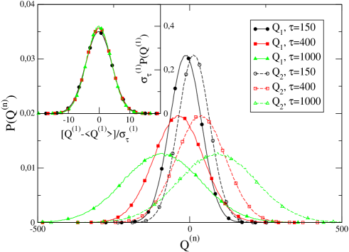
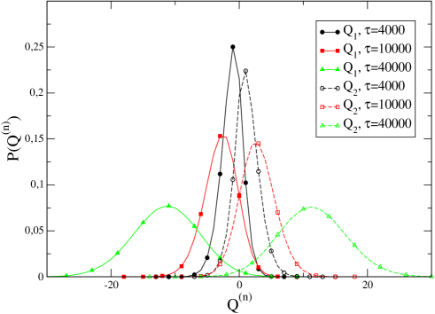
Figure 1: Upper panel ($T_{1},T_{2}>T_{c}$): Heat PDs for $\mathcal{Q}^{(1)}$ (on the left) and $\mathcal{Q}^{(2)}$ (on the right) for a system with $T_{1}=2.9,T_{2}=3$, size 10x10 and $t_{F}=6\cdot 10^{8}$ MCS. In the inset $\sigma^{(1)}_{\tau}\mathcal{P}(\mathcal{Q}^{(1)}({\tau}))$ is plotted against $(\mathcal{Q}^{(1)}(\tau)-\langle\mathcal{Q}^{(1)}(\tau)\rangle)/\sigma^{(1)}_{\tau}$. Curves for different $\tau$ collapse on a Gaussian mastercurve. Lower panel ($T_{1},T_{2}<T_{c}$): Same kind of plot for $T_{1}=1,T_{2}=1.3$, size 10 x 10 and $t_{F}=10^{9}$ MCS. The skewness of the distributions (see text) is equal to 2.35, 0.589, 0.11 for the cases $\tau=4000,10000,40000$ respectively.

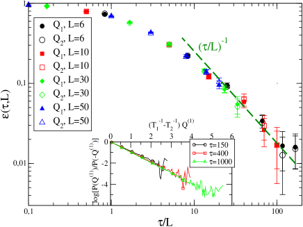
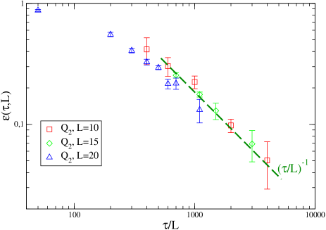
Figure 2: Same parameters of Fig. 1 (different sizes). Upper Panel ($T_{1},T_{2}>T_{c}$): $\epsilon(\tau,L)$ is plotted against $\tau/L$ for different $L$. Inset: $\log\left[\mathcal{P}(\mathcal{Q}^{(1)}(\tau))/\mathcal{P}(-\mathcal{Q}^{(1)}(\tau))\right]$ is plotted against $(1/T_{1}-1/T_{2})\mathcal{Q}^{(1)}(\tau)$. Lower panel ($T_{1},T_{2}<T_{c}$): $\epsilon^{(2)}$ is plotted against $\tau/L$ for different $L$.

The typical behavior of the heat probability distribution (PD) is reported in the upper panel of Fig.1 for the case with static coupling to the baths, single–spin–flip with Metropolis transition rates, $T_{1}=2.9$, $T_{2}=3$, and a square geometry with $L=M=10$ (Much larger sizes are not suitable because trajectories with a heat of opposite sign with respect to the average value would be too rare). As expected, $\mathcal{Q}^{(1)}(\tau)$ ($\mathcal{Q}^{(2)}(\tau)$) is on average negative (positive) and the relation $<\mathcal{Q}^{(1)}(\tau)>+<\mathcal{Q}^{(2)}(\tau)>=0$ is verified. Regarding the shape of the PD, due to the central limit theorem, one expects a gaussian behavior for $\tau$ greater than the (microscopic) relaxation time (in this case it is of few MCS ($\sim 5$)), namely $\mathcal{P}(\mathcal{Q}^{(n)}({\tau}))=(2\pi)^{-1/2}(\sigma^{(n)}_{\tau})^{-1}\exp[-\frac{(\mathcal{Q}^{(n)}(\tau)-\langle\mathcal{Q}^{(n)}(\tau)\rangle)^{2}}{2(\sigma^{(n)}_{\tau})^{2}}]$, with $\langle\mathcal{Q}^{(n)}(\tau)\rangle\sim\tau$ and $\sigma^{(n)}_{\tau}\sim\sqrt{\tau}$. This form is found with good accuracy, as shown in the inset of Fig. 1, where data collapse of the curves with different $\tau$ is observed by plotting $(\sigma^{(1)}_{\tau})^{1/2}\mathcal{P}(\mathcal{Q}^{(1)}({\tau}))$ against $(\mathcal{Q}^{(1)}(\tau)-\langle\mathcal{Q}^{(1)}(\tau)\rangle)/\sigma^{(1)}_{\tau}$.

In order to study the FR (1), we plot the logarithm of the ratio $\mathcal{P}(\mathcal{Q}^{(n)}(\tau))/\mathcal{P}(-\mathcal{Q}^{(n)}(\tau))$ as a function of $\Delta\beta^{(n)}\mathcal{Q}^{(n)}(\tau)$, see Fig. 2 (inset). For every value of $\tau$ the data are well consistent with a linear relationship (however, for large values of the heat the statistics becomes poor), in agreement with the gaussian form of the PDs. To verify the FR (1), the slopes of the plot

$$D^{(n)}(\tau)=\frac{\ln{\frac{\mathcal{P}(\mathcal{Q}^{(n)}(\tau))}{\mathcal{P}(-\mathcal{Q}^{(n)}(\tau))}}}{\mathcal{Q}^{(n)}(\tau)\Delta\beta^{(n)}}$$ (3)

must tend to 1 when $\tau\to\infty$. We show in Fig.2 the behavior of the distance $\epsilon^{(n)}=1-D^{(n)}(\tau)$ from the asymptotic behavior, for the case with static coupling to the baths. This quantity indeed goes to zero for large $\tau$ (the same is found for dynamic couplings). $\epsilon^{(n)}$ depends in general on the temperatures, the geometry of the system and on $\tau$. Its behavior can be estimated on the basis of the following argument.

In systems as the ones considered in this Letter, where generalized detail balance BD holds, the ratio between the probability of a trajectory in configuration space, given a certain intial condition, and its time reversed reads

$$\frac{\mathcal{P}(traj)}{\mathcal{P}(-traj)}=e^{\mathcal{Q}^{(n)}(\tau)\Delta\beta^{(n)}-\frac{\Delta E}{T_{n^{\prime}}}},$$ (4)

where $\Delta E=\mathcal{Q}^{(1)}(\tau)+\mathcal{Q}^{(2)}(\tau)$ is the difference between the energies of the final and initial state, and $n^{\prime}\neq n$. For systems with bounded energy, Eq. (4) is the starting point BD for obtaining the FR (1) in the large-$\tau$ limit. Since ${\mathcal{Q}}^{(n)}(\tau)$ increases with $\tau$ while $\Delta E$ is limited, in fact, the latter can be asymptotically neglected and, after averaging over the trajectories, the FR (1) is recovered. Keeping $\tau$ finite, instead, from Eqs. (3,4) one has that for the considered trajectory the distance of the slope from the asymptotic value is

$$\epsilon^{(n)}(traj)\simeq\frac{\Delta E}{T_{n^{\prime}}\mathcal{Q}^{(n)}(\tau)\Delta\beta^{(n)}}.$$ (5)

We now assume that the behavior of $\epsilon^{(n)}$ can be inferred by replacing $\Delta E$ and $\mathcal{Q}^{(n)}(\tau)$ with their average values whose behavior can be estimated by scaling arguments. Starting with the average of $\mathcal{Q}^{(n)}(\tau)$, we argue that this quantity is proportional to $N_{flux}\tau$, $N_{flux}$ being the number of couples of nearest neighbor spins interacting with baths at different temperatures. This is because between these spins a neat heat flux occurs. In the model with static coupling to the baths one has $N_{flux}\propto L$. With dynamic coupling, instead, since every spin in the system can feel one or the other temperature, one has $N_{flux}\propto N$. Concerning the average of $\Delta E$, this is an extensive quantity proportional to the number $N$ of spins. We then arrive at

$$\epsilon^{(n)}\simeq(T_{n^{\prime}}\Delta\beta^{(n)})^{-1}\,\left\{\begin{array}[]{ll}L\tau^{-1}\qquad$static coupling to baths$\\ \tau^{-1}\qquad$dynamic coupling to baths.$\end{array}\right.$$ (6)

This result is expected to apply for sufficiently large $\tau$ when our scaling approach holds.

We remind that finite-$\tau$ corrections have been shown to be of order $1/\tau$ for the classes of dynamical systems considered in GC95 ; MR03 . The same is found in Zon for models based on a Langevin equation nota , in cases corresponding to the experimental setup of a resistor in parallel with a capacitor cili . Faster decays ($\sim 1/\tau^{2}$) have been predicted for other topologies of circuits Zon . On the other hand, FRs in transient regimes, which are not considered in this Communication, are exact at any $\tau$ ($\epsilon=0,\forall\tau$) Jarzynski00 .

In our model with static couplings the data of Fig. 2 confirm the prediction of the argument above: curves with different $L$ collapse when plotted against $x=\tau/L$ and $\epsilon^{(n)}\propto x^{-1}$ for sufficiently large $\tau$. Similar behaviors have been found by varying the geometry (we also considered rectangular lattices with $L>M$), transition rates, and dynamics. The scaling prediction (6) has been verified for the Ising model with Kawasaki dynamics and squared geometry with $L=10,20,40$, and in the case of the system dynamically coupled to the heat baths for sizes between $L=6$ and $L=60$.

$\mathbf{T_{1},T_{2}<T_{c}}$

Let us first recall the behavior of the Ising model in contact with a single bath at temperature $T<T_{c}$. When $N=\infty$ the system is confined into one of the two pure states which can be distinguished by the sign of the magnetization $m(T)=(1/N)\sum_{i=1}^{N}\sigma_{i}$. This state is characterized by a microscopic relaxation time $\tau_{eq}(T)$ which is related to the fast flip of correlated spins into thermal islands with the typical size of the coherence length. At finite $N$, instead, genuine ergodicity breaking does not occur. The system still remains trapped into the basin of attraction of the pure states but only for a finite ergodic time $\tau_{erg}(N,T)$, which diverges when $N\to\infty$ or $T\to 0$. Then, as compared to the case $T>T_{c}$, there is the additional timescale $\tau_{erg}(N,T)$, beside $\tau_{eq}(T)$, which can become macroscopic. This whole phenomenology is reflected by the behavior of the autocorrelation function $C(t-t^{\prime})=\langle\sum_{i}\sigma_{i}(t^{\prime})\sigma_{i}(t)\rangle$. When, for large $N$, the two timescales $\tau_{eq}(T),\tau_{erg}(N,T)$ are well separated, it first decays from $C(0)=1$ to a plateau $C(t-t^{\prime})=m(T)^{2}$ on times $t-t^{\prime}\simeq\tau_{eq}(T)$, due to the fast decorrelation of spins in thermal islands. The later decay from the plateau to zero, observed on a much larger timescale $t-t^{\prime}\simeq\tau_{erg}(N,T)$, signals the recovery of ergodicity. Notice also that, from the behavior of $C(t-t^{\prime})$ both the characteristic timescales can be extracted.

The same picture applies qualitatively to the case of two subsystems in contact with two thermal baths, where each systems is trapped in states with broken symmetry for a time $\tau_{erg}(N,T_{n})$ ($\tau_{erg}(N,T_{1})>\tau_{erg}(N,T_{2})$ since $T_{1}<T_{2}$), which can be evaluated from the autocorrelation functions $C^{(n)}(t-t^{\prime})=\langle\sum_{i}\sigma_{i}^{(n)}(t)\sigma_{i}^{(n)}(t^{\prime})\rangle$, where $\sigma_{i}^{(n)}$ denote spins in contact with the bath at $T=T_{n}$. Since the FR is expected for $\tau$ larger than the typical timescales of the system, it is interesting to study the role of the additional timescales $\tau_{erg}(N,T_{n})$ on the FR. By varying $T_{1},T_{2}$ and $N$ appropriately one can realize the limit of large $\tau$ in the two cases with i) $\tau\ll\tau_{erg}(N,T_{2})$ or ii) $\tau\gg\tau_{erg}(N,T_{1})$. In case i), in the observation time-window $\tau$, the system is practically confined into broken symmetry states while in case ii) ergodicity is restored. Not surprisingly, in the latter case, we have observed a behavior very similar to that with $T_{1},T_{2}>T_{c}$. The PDs for the case i) are shown in the lower panel of Fig. 1. The distributions are more narrow and non Gaussian. We calculated the skewness of the distributions defined as $<(\mathcal{Q}(\tau)-<\mathcal{Q}(\tau)>)^{3}>/<(\mathcal{Q}(\tau)-<\mathcal{Q}(\tau)>)^{2}>^{3/2}$. This quantity is zero for gaussian distributions while for the case of the lower panel of Fig. 1 we found values different from zero which have been reported in the caption of the figure. This data show that the PDs slowly approach a Gaussian form increasing $\tau$. Moreover, differently than in the high temperature case, an asymmetry between the distributions of $\mathcal{Q}^{(1)}(\tau)$ and $\mathcal{Q}^{(2)}(\tau)$ can be observed.

Regarding the slopes $D^{(n)}(\tau)$, they converge to 1 also in this case even if the times required to reach the asymptotic behavior are much longer than in the high temperature case (but always smaller than $\tau_{erg}(N,T_{2})$). This suggests that the FR (1) holds even in states where ergodicity is broken and that the presence of the macroscopic timescales $\tau_{erg}(N,T_{n})$ does not affect the validity of the FR in this system. Regarding the scaling of $\epsilon^{(n)}$, the data are much more noisy than in the case $T_{1},T_{2}>T_{c}$, particularly for $\epsilon^{(1)}$. Despite this, the data presented in the lower panel of Fig.2 for $\epsilon^{(2)}$ are consistent with the scaling (6) suggesting that it is correct also in this situation.

In this Letter we have considered different realizations of Ising models coupled to two heat baths at different temperature. We studied the fluctuation behavior of the heat exchanged with the thermostats and found that the FR (1) is asymptotically verified in all the cases considered. We also analyzed the effects of finite time corrections and their scaling behavior. The picture is qualitatively similar in the high and low temperature phases, although very different timescales are required to observe the asymptotic FR.

- (1) D. J. Evans, E. G. D. Cohen and G. P. Morriss, Phys. Rev. Lett. 71, 2401 (1993).
- (2) D. J. Evans and D. J. Searles, Phys. Rev. E 50, 1645 (1994).
- (3) G. Gallavotti and E.G.D. Cohen, J. Stat. Phys. 80, 931 (1995); Phys. Rev. Lett. 74 2694 (1995).
- (4) C. Jarzynski, Phys. Rev. Lett. 78, 2690 (1997).
- (5) J. Kurchan, J. Phys. A 31, 3719 (1998).
- (6) J.L. Lebowitz and H. Spohn, J. Stat. Phys. 95, 333 (1999).
- (7) C. Maes, J. Stat. Phys. 95, 367 (1999).
- (8) G.E. Crooks, Ph.D. Thesis, University of California at Berkeley (1999); Phys. Rev. E 60, 2721 (1999).
- (9) T. Hatano and S. Sasa, Phys. Rev. Lett. 86, 3463 (2001).
- (10) R. van Zon and E.G.D. Cohen, Phys. Rev. Lett. 91, 110601 (2003).
- (11) U. Seifert, Phys. Rev. Lett. 95, 040602 (2005).
- (12) For recent reviews see e.g. R.J. Harris and G.M. Schütz, J. Stat. Mech. P07020 (2007); G. Gallavotti, arXiv:0711.2755; F. Ritort, Adv. in Chem. Phys. 137, 31 (2008); L. Rondoni and C. Mejia-Monasterio, Nonlinearity 20, R1 (2007); R. Chetrite and K. Gawedzki, arXiv:0707.2725.
- (13) C. Bustamante, J. Liphardt and F. Ritort, Phys. Today 58, 43 (2005).
- (14) G.M.Wang, E.M.Sevick, E. Mittag, D. J. Searles, and D.J. Evans, Phys. Rev. Lett. 89 050601 (2002).
- (15) N. Garnier and S. Ciliberto, Phys. Rev. E 71 060101, (2005).
- (16) T. Bodineau and B. Derrida, C.R. Physique 8, 540 (2007).
- (17) S. Lepri, R.Livi, A. Politi, Physica D 119 140 (1998).
- (18) P. Visco, J. Stat. Mech. P06006 (2006).
- (19) C. Jarzynski and D.K. Wojcik, Phys. Rev. Lett. (2007).
- (20) V. Lecomte, Z. Racz and F. van Wijland, J. Stat. Mech., P02008 (2005).
- (21) M.J. de Oliveira, J.F.F. Mendes and M.A. Santos, J.Phys.A 26, 2317 (1993).
- (22) J.M. Drouffe and C. Godrèche, J.Phys.A 32, 249 (1999); F. Sastre, I. Dornic, H. Chatè, Phys. Rev. Lett. 91, 267205 (2003); N. Andrenacci, F. Corberi, and E. Lippiello Phys. Rev. E 73, 046124 (2006).
- (23) L.Rondoni and G.P. Morriss, Open Sist. & Information Dynam. 10 105 (2003).
- (24) R. van Zon, S. Ciliberto, and E.G.D Cohen, Phys.Rev. Lett. 92, 130601 (2004).
- (25) In the system studied in Zon , corrections have been predicted for any range of work fluctations and only for some range of heat fluctuations. Moreover, differently than in our case, the slope 1 in work fluctuations is reached from above, i.e. is negative.
- (26) See e.g. C. Jarzynski, J. Stat. Phys. 98, 77 (2000).