Combustion dynamics in steady compressible flows

Abstract

We study the evolution of a reactive field advected by a one-dimensional compressible velocity field and subject to an ignition-type nonlinearity. In the limit of small molecular diffusivity the problem can be described by a spatially discretized system, and this allows for an efficient numerical simulation. If the initial field profile is supported in a region of size $\ell<\ell_{c}$ one has quenching, i.e., flame extinction, where $\ell_{c}$ is a characteristic length-scale depending on the system parameters (reacting time, molecular diffusivity and velocity field). We derive an expression for $\ell_{c}$ in terms of these parameters and relate our results to those obtained by other authors for different flow settings.

Front propagation in reaction-transport systems is a widely studied topic in both scientific and applicative fields such as the dynamics of biological populations, chemical reactions in fluids and flame propagation in gases Williams ; Abraham ; Epstein ; rmv88 .

From the mathematical point of view, these phenomena can be modeled in terms of partial differential equations describing the evolution of both the concentrations of the reacting species, and the velocity field Peters ; xin2000 . Though in principle these equations are coupled, a simplification comes from the assumption of no back-reaction of the reactants concentration on the velocity field. In this passive limit one can use an advection-reaction-diffusion equation. The most compact model considers the evolution of a single scalar field $\theta({\bf x},t)$ representing the fractional concentration of products, or a normalized temperature in the case of combustion processes, taking values in the interval $[0,1]$.

The interest, and the difficulty, in the treatment of this subject is due to the effect of advection on the reaction process: theoretical studies Constantin1 ; Pomeau ; Yakhot , numerical simulations Constantin2 ; acvv01 ; kn04 and laboratory experiments Bradley ; srby92 show that the propagation speed of the front is significantly altered by the presence of the fluid flow. When an infinite reservoir of inert material is present, advection enhances the speed of travelling waves. On the other hand, if the initial condition is localized in a region of finite size, for a certain class of reaction dynamics, the combined action of diffusion and advection might reduce and eventually suppress front propagation. It is then interesting to study how the critical size of the initial support, below which the reactive process quenches, depends on the characteristics of both the velocity field and the reaction dynamics Constantin1 ; Constantin2 .

In this letter we study the quenching phenomenon, or flame extinction in combustion terminology, in a one-dimensional compressible velocity field in the limit of small molecular diffusivity. The reactive dynamics is modeled by means of an ignition-like nonlinearity, that is a reaction term with a threshold value $\theta_{c}$, such that if $\theta<\theta_{c}$ no reaction takes place. We derive a relation between the critical size of the initial condition width and the relevant parameters of the problem, namely the reaction time, the reaction threshold value and the combined effect of diffusivity and flow intensity. In the end we will compare our results with those obtained by other authors in different contexts, i.e., reactive field advected by bidimensional incompressible velocity fields Constantin1 .

I Model

Consider the usual advection-reaction-diffusion problem

$$\partial_{t}\theta+\mbox{\boldmath$\nabla$}\cdot\left({\bf u}\,\theta\right)=D_{0}\nabla^{2}\theta+{1\over\tau}f(\theta),$$ (1)

where ${\bf u}({\bf x},t)$ is a given compressible velocity field, $D_{0}$ is the molecular diffusivity and $f(\cdot)$ the reactive term with its characteristic time $\tau$. For the sake of simplicity we adopt a one-dimensional stationary model with velocity field:

$$u(x)=U_{0}\sin\left({\pi x\over L}\right)\,.$$ (2)

Let us first discuss the system dynamics in absence of reaction. The Lagrangian equation

$${{\mathrm{d}}x\over{\mathrm{d}}t}=u(x)$$ (3)

has the following stable fixed points (for $U_{0}>0$) $x=\pm L,\pm 3L,\ldots,\pm(2n-1)L,\ldots$ while $x=0,\pm 2L,\ldots,\pm 2nL,\ldots$ are unstable. In absence of reaction the field $\theta$ will concentrate around the stable fixed points $x_{n}=(2n-1)L$ with $n=0,\pm 1,\pm 2,\ldots$ and, essentially, one has a random walk among the points $x_{n}$. The characteristic time of jumping is determined by $U_{0}$ and $D_{0}$.

In a suitable range of values of $U_{0}$ and $D_{0}$ the field $\theta(x,t)$ is well peaked around $x_{n}$, so we can introduce the variable $\theta_{n}$:

$$\theta_{n}(t)=\int_{x_{n}-L}^{x_{n}+L}\theta(x,t){\mathrm{d}}x=\int_{x_{n}-\delta}^{x_{n}+\delta}\theta(x,t){\mathrm{d}}x\,,$$ (4)

where $\delta\ll L$. It is not difficult to write down the evolution equation for $\theta_{n}(t)$:

$$\theta_{n}(t+\Delta t)=\sum_{j}P_{j\to n}^{(\Delta t)}\theta_{j}(t)$$ (5)

where

$$P_{n\to n}^{(\Delta t)}=1-2W\Delta t\qquad P_{n\to n-1}^{(\Delta t)}=P_{n\to n+1}^{(\Delta t)}=W\Delta t,$$ (6)

and $W$ is a function of $U_{0}$ and $D_{0}$, i.e., the escape rate of a Brownian particle from a potential well. For small $D_{0}$ it is possible to show that $\ln W\sim-{U_{0}\over D_{0}}$, which is the celebrated Kramers formula Gardiner . For generic $D_{0}$ and periodic velocity field $u(x)$ it is not difficult to have good numerical estimate of $W$.

In equation (5) both time and space are discrete. However, while the time discretization is merely due to numerical reasons, the discretization of space is a consequence of compression, and in the limit of small $D_{0}$ (and not small $U_{0}$) equation (5) is a very good approximation. It is worth to note that the same kind of approximation can be found in solid state physics in the so called Anderson “tight binding” model Anderson , where the electronic wave function is assumed to be localized around the nuclei.

In presence of reaction eq. (5) changes into

$$\theta_{n}(t+\Delta t)=G_{\Delta t}\left(\sum_{j}P^{(\Delta t)}_{j\to n}\theta_{j}(t)\right)\,,$$ (7)

where $G_{\Delta t}(\theta)$ is an assigned reaction map. For a discussion on how to obtain the previous rule from the basic equation (1) see acvv01 ; Mancinelli .

The shape of the reaction map $G_{\Delta t}(\theta)$ depends on the underlying chemical model. For an autocatalytic reaction (the FKPP class), characterized by an unstable fixed point in $\theta=0$ and a stable one in $\theta=1$, one has: $G_{\Delta t}(\theta)=\theta+\theta(1-\theta)\Delta t/\tau.$ For ignition-type class, instead, the reactive map reads:

$$G_{\Delta t}(\theta)=\left\{\begin{array}[]{lll}\theta&&0\leq\theta\leq\theta_{c}\\ \theta+(\theta-\theta_{c})(1-\theta){\displaystyle{\Delta t\over\tau}}&&\theta_{c}<\theta\leq 1.\end{array}\right.$$ (8)

We expect from known results xin2000 , valid for the time-continuous PDE (1) that, at a qualitative level, the detailed shape of $G_{\Delta t}(\theta)$ is not very relevant, within a given class of nonlinearities (e.g. FKPP or ignition-like). This expectation is confirmed by numerical simulations.

II Numerical results

Let us now present the results of numerical computations for the system (7). For the sake of simplicity we consider a spacing $\Delta x=1$ (the distance between two fixed point of eq. (3)); the lattice size being $L_{x}\leq 4\cdot 10^{4}$. We use a time step $\Delta t\leq 10^{-2}$ and an initial condition localized around $n=0$, $\theta_{n}(0)=\Theta_{n}$, where

$$\Theta_{n}=\left\{\begin{array}[]{l}1\qquad{\mathrm{for}}\,\,\,|n|\leq{\ell\over 2}\\ 0\qquad{\mathrm{for}}\,\,\,|n|>{\ell\over 2}.\end{array}\right.$$ (9)

A useful observable to focus on is the spatial integral of the scalar field $\theta_{n}$, which represents the total burnt area in the case of ideal fronts; therefore we compute its analogue on the lattice, expressed by the quantity

$$Q(t)=\sum_{n=-\infty}^{+\infty}\theta_{n}(t)\,.$$ (10)

In absence of quenching we have an asymptotic linear growth of $Q(t)$, that is

$$Q(t)\simeq 2v_{f}t\qquad\mbox{for large }t\,,$$ (11)

where $v_{f}$ is the front speed. The coefficient 2 is here due to the fact that with our choice for the initial condition two symmetric fronts develop. In the case of autocatalytic reaction term we obtain (for large $\tau$ and $W$) the expected result valid for the continuous FKPP limit $v_{f}=2\sqrt{W/\tau}$.

III Ignition reaction term

Now we consider the ignition case with the reaction term (8) and investigate the possibility of quenching of the reactive dynamics. This could occur for large values of the threshold density $\theta_{c}$ and/or for narrow initial conditions, and also depends on the reaction time, $\tau$, and on the combined effects of molecular diffusivity and advective flow, $W$. As a first example, we show in Figure 1 the system dynamics at varying the initial width $\ell$. The quenching appearance can be detected following the behaviour in time of $Q$ and $v_{f}$. If the initial condition is narrow enough, after a transient the growth of $Q$ is arrested and correspondingly the front speed goes to zero. For larger values of $\ell$ propagation takes place with the asymptotic time behaviour $Q\simeq 2v_{f}t$. In such a way it is possible to determine a critical length $\ell_{c}$ separating the two regimes:

$\ell<\ell_{c}$	$\Rightarrow$	$\theta(x,t\rightarrow\infty)\rightarrow 0$	(quenching)
$\ell>\ell_{c}$	$\Rightarrow$	$\theta(x,t\rightarrow\infty)\rightarrow 1$	(propagation).

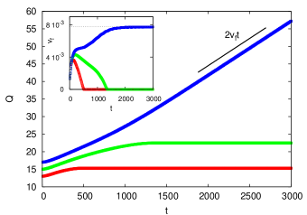
Figure 1: (color online) $Q$ as a function of the time $t$ for $\theta_{c}=0.6$, $W=0.1$ and $\tau=50$. The initial condition widths are $\ell=14,16,18$ from bottom to top. In the propagating case ($\ell=18$) $Q\simeq 2v_{f}t$ for large times. Inset: front speed $v_{f}$ vs. $t$.

The critical value of the initial width will depend on the relevant physical parameters of the problem: $W$, $\tau$ and $\theta_{c}$. In order to investigate this point we perform two types of numerical experiments. In the first one (experiment A) we keep the reaction time $\tau$ fixed and vary the escape rate $W$ for a given set of values of $\theta_{c}$. In the second one (experiment B), the situation is reversed, namely, for the same values of $\theta_{c}$, we study how $\ell_{c}$ varies with $\tau$ when $W$ is kept constant. Irrespective of the specific value of the threshold concentration, in both cases A and B we find a square-root relation between $\ell_{c}$ and the product $W\tau$:

$$\ell_{c}=F(\theta_{c})\sqrt{W\tau}$$ (12)

where $F(\theta_{c})$ is a constant factor containing the dependence on $\theta_{c}$ (see Figure 2).

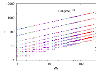
Figure 2: (color online) Critical width of the initial condition as a function of the product $W\tau$ for data sets coming from both experiments A ($\tau=10,\tau=50$) and B ($W=0.1,W=0.25$). The different colours correspond to the four different experimental settings and symbol types to different values of $\theta_{c}$; from bottom to top $\theta_{c}=0.3,0.4,...,0.9,0.95$.

Relation (12) can be derived by a dimensional argument. In the continuum limit of the lattice model,i.e., $L_{x}\gg\Delta x$, the system can be regarded as a pure reaction-diffusion system with diffusivity equal to $D=W\Delta x^{2}=W$, since we use $\Delta x=1$. Then, the only possibility to build a length-scale with the quantities $W\equiv D$, $\tau$ and $\theta_{c}$ is $\sqrt{W\tau}F(\theta_{c})$, where $F$ is a nondimensional function of the threshold concentration. If the initial width of the burnt area is smaller than this, then the “equivalent diffusion”, i.e., the combined effects of diffusion and velocity field, will be efficient enough to spread the majority of the inert material below the concentration threshold on a reactive time-scale and, consequently, to quench the reaction. The above results are summarized in Figure 2, where $\ell_{c}$ is plotted against $W\tau$, and Figure 3 where all data are collapsed onto a single curve showing the universality of the square-root dependence.

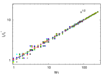
Figure 3: (color online) Collapse of the data reported in Fig. 2 showing the universality of the square-root law. In the vertical axis we plot $\ell_{c}/\ell_{c}^{*}$ where $\ell_{c}^{*}$ is computed for $W\tau=1$.

A natural question arises, concerning the shape of the function $F(\theta_{c})$ appearing in eq. (12). Its values, measured in experiments of type A and B, are reported in Figure 4. The perfect superposition of data corresponding to different experimental settings reflects the robustness of the dimensional estimate (12), and the fact that the dependence on $\theta_{c}$ can be found only in the prefactor, $F(\theta_{c})$.
In order to clarify the dependence on $\theta_{c}$ we consider an ansatz based on the following very general physical hypothesis:

(i)

$F(\theta_{c})$ is a non-negative function, monotonically increasing with $\theta_{c}\in[0,1]$

(ii)

$F(\theta_{c})\rightarrow 0$ when $\theta_{c}\rightarrow 0$

(iii)

$F(\theta_{c})\rightarrow\infty$ when $\theta_{c}\rightarrow 1$

(iv)

$F(\theta_{c})$ is analytic for $\theta_{c}\neq 1$.

Some comments are in order. Hypothesis (ii) and (iii) correspond to the physical expectation that when the threshold is very small the reaction proceeds and when it is very large it quenches, respectively. Moreover, when $\theta_{c}\rightarrow 0$ the system clearly cannot exhibit quenching, since in that limit the reaction term (8) reduces to the discrete-time version of the autocatalytic FKPP term $G_{\Delta t}(\theta)=\theta+\theta(1-\theta)\Delta t/\tau$, which is known to always give rise to front propagation Rocquejoffre1 ; Rocquejoffre2 . Hypothesis (iv) states that the only singular point we expect is $\theta_{c}=1$.

According to the above hypothesis, we can Laurent-expand the function $F(z)$ around the point $z=1$:

$$F(z)=a_{0}+{a_{-1}\over{1-z}}+{a_{-2}\over{(1-z)^{2}}}+...=\sum_{k=0}^{\infty}{a_{-k}\over{(1-z)^{k}}}$$ (13)

The expansion will be truncated at a certain order $\alpha$ if all the coefficients $a_{-k}$ with $k>\alpha$ are zero, that is if the singularity is a pole of order $\alpha$. The numerics suggest that indeed the point $z=1$ is a pole of order $\alpha=2$. In other words:

$$\lim_{z\rightarrow 1}(1-z)^{\alpha}F(z)=0\quad\mbox{for}\quad\alpha\geq 3$$ (14)

and therefore we conjecture the ansatz

$$F(z)=a_{0}+{a_{-1}\over{1-z}}+{a_{-2}\over{(1-z)^{2}}}.$$ (15)

Though this is formally a 3-parameter family of functions, one of the parameters can be eliminated imposing the physical constraint $F(z=0)=0$ (hypothesis (ii)). In the end, by doing so, we get the following expression for $F(\theta_{c})$:

$$F(z)=a_{0}{z\over{1-z}}\left(1+{a_{-2}\over a_{0}}{1\over{1-z}}\right).$$ (16)

In this form, the role of the extremal points $\theta_{c}=0,1$ is evident: if $\theta_{c}\rightarrow 0$ then $F$ vanishes and so does $\ell_{c}$, that is, propagation always prevails. On the contrary, when $\theta_{c}\rightarrow 1$ the divergence of $F$ implies that of the critical width of the initial condition, corresponding to quenching of the reaction independently of the fixed values of $W$ and $\tau$. Therefore, in a practical situation, an improved estimate of the scaling relation $\ell_{c}\sim\sqrt{W\tau}$ can be obtained by using the heuristic expression (16). In Figure 4 we report a comparison between a fit with the function in eq. (16) and the numerical results; the agreement is rather good, confirming our conjecture.

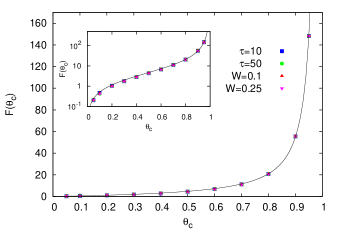
Figure 4: (color online) Plot of the function $F(\theta_{c})$ for experiments A ($\tau=10$, $\tau=50$) and B ($W=0.1$, $W=0.25$). The solid line is a fit with a function corresponding to the second order expansion around the singularity $z=1$: $F(z)=a_{0}{z\over{1-z}}\left(1+{a_{-2}\over a_{0}}{1\over{1-z}}\right)$; $a_{0}\simeq 4.39$, $a_{-2}\simeq 0.17$; for the piecewise-linear reaction map $\tilde{G}_{\Delta t}$ (see eq. (17) in the text) $a_{0}\simeq 4.88$, $a_{-2}\simeq 0.20$. Inset: semilogarithmic plot of the same function.

In order to check the robustness of the above result we considered another ignition reaction map in place of eq. (8)

$$\tilde{G}_{\Delta t}(\theta)=\left\{\begin{array}[]{lr}\theta&0\leq\theta\leq\theta_{c}\vspace{0.2truecm}\\ \theta+{\displaystyle{{1-\theta_{c}}\over{2\tau}}}\Delta t(\theta-\theta_{c})&\theta_{c}<\theta\leq\theta_{*}\vspace{0.2truecm}\\ \theta+{\displaystyle{{1-\theta_{c}}\over{2\tau}}}\Delta t(1-\theta)&\theta_{*}<\theta\leq 1\end{array}\right.$$ (17)

where $\theta_{*}=(1+\theta_{c})/2$. Numerical simulations indeed demonstrate (results not shown) that the scaling behaviour of $\ell_{c}$ and the shape of the function $F(\theta_{c})$ do not significantly change.

It is natural to wonder about the existence (or not) of a link between the critical length $\ell_{c}$ and the characteristic front thickness $\xi\propto\sqrt{W\tau}$. We remind that $\xi$ can be defined from the asymptotic shape of the propagating front. In order to guarantee front propagation one can assume as initial condition $\theta=1$ for $x<0$ ($x>0$ for the symmetric case), which implies an infinite reservoir of burnt material. A first question is whether the front, in the case of a compressible velocity field and with ignition reaction term, has a different shape from that of the paradigmatic FKPP model. It is known from theoretical results (see, e.g., Aronson ) that the standard FKPP front shape is exponential, i.e., for $x\gtrsim v_{0}t$ one has $\theta(x,t)\sim\exp[-(x-v_{0}t)/\xi_{0}]$, where $v_{0}=2\sqrt{D/\tau}$ and $\xi_{0}=\sqrt{D\tau}$ are the FKPP front speed and length, respectively.

In the inset of Figure (5) the shape of the right propagating front is shown. Its exponential shape is well evident. This result allows us to use the following expression for the front shape:

$$\theta(x,t)\propto\exp\left(-{x-v_{f}t\over\xi}\right)\,,$$ (18)

from which the front length $\xi$ can be computed.
To investigate the link between $\xi$ and $\ell_{c}$ we measured the front length at varying $\theta_{c}$. In Figure 5 it is possible to observe that for $\theta_{c}\gtrsim\theta^{*}\approx 0.3$ one has $\ell_{c}\approx\xi$. On the contrary, for $\theta_{c}\lesssim\theta^{*}$, $\ell_{c}$ is smaller than $\xi$. In particular for very small values of $\theta_{c}$ one has $\ell_{c}\to 0$ while $\xi\to\xi_{0}=\sqrt{W\tau}\neq 0$. This is indicative of the fact that the quenching phenomenon is not simply related to the (usual) features of the front.

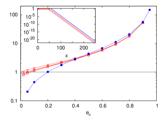
Figure 5: (color online) Plot of the rescaled front thickness and the function $F(\theta_{c})$. The symbols $\square$, $\circ$, $\bigtriangledown$ and $\bigtriangleup$ indicate the rescaled front thickness in the cases $W=0.1$ and $\tau=10$, $W=0.25$ and $\tau=10$, $W=0.25$ and $\tau=2$, $W=0.1$ and $\tau=2$, respectively. The symbol $\bullet$ indicates the function $F(\theta_{c})$. The straight line is the $\xi_{0}$ value in the case of a pure FKPP process. In the inset it is shown the right side of the front shape.

IV Conclusions

Let us now conclude with some general considerations and a comparison of our results with others obtained for incompressible bidimensional velocity fields.
As first, we note that for $\Delta x\to 0$ the rule (7) is, with a suitable rescaling of the parameters, nothing but the finite difference discretization algorithm to solve eq. (1) with ${\bf u}=0$. Therefore, our numerical results are also related to the quenching problem of the pure reaction-diffusion system with ignition-like nonlinearities. For the latter case there exists a theoretical prediction of the system behaviour Kanel ; Zlatos that is in good agreement with our results.

Moreover, in refs. Constantin1 ; Constantin2 Constantin and co-workers performed detailed numerical simulations of the quenching problem in the case of slow reaction in two-dimensional incompressible velocity fields, in particular for

• shear flow of typical intensity $U$,

• cellular flow of typical intensity $U$,

obtaining $\ell_{c}\sim U$ in case a) and $\ell_{c}\sim U^{1\over 4}$ in case b). Such a conclusion can be easily related to our results. In fact, in the slow reaction limit the long time and large scale behaviour of (1) can be written as

$$\partial_{t}\theta=D^{\mathrm{eff}}\nabla\theta+{1\over\tau}f(\theta)$$ (19)

where $D^{\mathrm{eff}}$ depends (often in a non-trivial way) on the velocity field ${\bf u}$ (see, e.g., acvv01 ). Therefore, we can use the previous result (on the connection between (7) and the pure reaction-diffusion problem without velocity field) and conclude that $\ell_{c}\sim\sqrt{D^{\mathrm{eff}}\tau}$. Using the well known result (see, e.g., acvv01 ) that $D^{\mathrm{eff}}\sim U^{2}$ for the shear flow (case a)) and $D^{\mathrm{eff}}\sim U^{1\over 2}$ for the cellular flow (case b)) one obtains the result of Constantin et al. Constantin1 ; Constantin2 .

In conclusion, we studied the quenching phenomenon of ignition-type reaction dynamics in a steady compressible flow. We developed a simplified lattice model based on a physically controllable localization approximation for the concentration field, which allows an efficient numerical implementation. The dependence of the critical initial condition width $\ell_{c}$ on the relevant parameters $W,\tau,\theta_{c}$ was established by means of numerical experiments and dimensional reasoning. Finally we compared our results with those obtained theoretically and numerically in different flow configurations.

- (1) F.A. Williams, Combustion Theory (Benjamin-Cummings, Menlo Park, CA, 1985).
- (2) E.R. Abraham, Nature 391, 577 (1998).
- (3) I.R. Epstein, Nature 391, 231 (1998).
- (4) J. Ross, S.C. Müller and C. Vidal, Science 240, 260 (1988).
- (5) N. Peters, Turbulent Combustion (Cambridge University Press, Cambridge, UK, 2000).
- (6) J. Xin, SIAM Review 42, 161 (2000).
- (7) P. Constantin, A. Kiselev and L. Ryzhik, Communications in Pure and Applied Mathematics 54, 1320 (2001).
- (8) B. Audoly, H. Berestycki and Y. Pomeau, C.R. Acad. Sci., Ser. IIb: Mec., Phys., Chim., Astron. 328, 255 (2000).
- (9) V. Yakhot, Combust. Sci. and Tech. 60, 191 (1988).
- (10) N. Vladimirova, P. Constantin, A. Kiselev, O. Ruchayskiy and Ryzhik L., Combust. Theory Modelling 7, 487 (2003).
- (11) M. Abel, A. Celani, D.Vergni and A. Vulpiani, Phys. Rev. E 64, 046307 (2001).
- (12) C.R. Koudella and Z. Neufeld, Phys. Rev. E 70, 026307 (2004).
- (13) D. Bradley, 24th Int. Symp. on Combustion, p 247 (Pittsburgh, PA: The Combustion Institute, 1992).
- (14) S.S. Shy, P.D. Ronney, S.G. Buclkey and V. Yakhot, 24th Int. Symp. on Combustion, p543 (Pittsburgh, PA: The Combustion Institute).
- (15) C.W. Gardiner, Handbook of Stochastic Methods (Springer, Berlin, 2004).
- (16) N.W. Ashcroft and N.D. Mermin, Solid State Physics (Saunders College, Philadelphia, 1976).
- (17) R. Mancinelli, D. Vergni and A. Vulpiani, Physica D 185, 175 (2003).
- (18) J.M. Rocquejoffre, Arch. Rational. Mech. Anal. 117, 119 (1992).
- (19) J.M. Rocquejoffre, Ann. Inst. Henri Poincaré Anal. Non Linéaire 14, 499 (1997).
- (20) D.G. Aronson and H.F. Weinberger, Adv. Math. 30, 33 (1978).
- (21) J.I. Kanel’, Mat. Sb. (N.S.) 65 (107), 398 (1964).
- (22) A. Zlatoš, Journal of the American Mathematical Society 19 (1), 251 (2005).