Solution of large linear systems with embedded network structure for a non-homogeneous network flow programming problem

Abstract

In the paper we consider the linear underdetermined system of a special type. Systems of this type appear in non-homogeneous network flow programming problems in the form of systems of constraints and can be characterized as systems with a large sparse submatrix representing the embedded network structure. We develop a direct method for finding solutions of the system. The algorithm is based on the theoretic-graph specificities for the structure of the support and properties of the basis of a solution space of a homogeneous system. One of the key steps is decomposition of the system. A simple example is regarded at the end of the paper.

Mathematics Subject Classification: 05C50, 15A03, 15A06, 65K05, 90C08, 90C35

Keywords: sparse linear system, underdetermined system, direct method, basis of a solution space of a homogeneous linear system, decomposition of a system, network, network support, spanning tree, fundamental system of cycles, characteristic vector

1 Introduction

The work on this paper was motivated, mainly, by the analysis of problems of non-homogeneous network flow optimization on large data files [1]-[3], [5]-[7]. Our main goal was to develop an effective (direct) method for solving large sparse systems of linear equations with embedded network structure, which appear naturally, e.g. as systems of constraints, in a broad class of non-homogeneous network flow programming problems.

The ’network nature’ of the regarded system allows keeping data in the matrix-free form in the computer memory. The formulae, derived within the paper, are written in the component (network) form to provide clear approaches towards developing computational algorithms using efficient data structures for graph representation [1].

The general idea of the method is based on the following key steps:

$\bullet$ Distinguishing between the network part of the system and the additional part. The network part of the system represents a network structure and corresponds to the network part of the system of main constraints of a non-homogeneous network flow programming problem [1], and is given, traditionally, by balance equations, written for the nodes of a network. The additional part of the system corresponds to the additional part of the system of main constraints and can have a general form. We start the solution by considering the network part of the system only.

$\bullet$ Introduction of the support of the network for a system. The term ’support of the network’ (also referred to as network support, or support) is borrowed from optimization theory [2], [3] and is used here for further compatibility with applications in problems of non-homogeneous network flow programming. The actual meaning in this paper is – a set of indices of variables (or, in the network terms, - a set of arcs) corresponding to columns, which form a basis minor of the matrix of a system. We study the support for the network part of the system, finding the correspondence between the columns of a basis minor and a family of spanning trees.

$\bullet$ Construction of a general solution for the network part of the system. We compute a basis of a solution space of the corresponding homogeneous system and interpret the basis vectors as characteristic vectors, entailed by non-support arcs. A simple approach for finding a partial solution of the (non-homogeneous) system is provided.

$\bullet$ Decomposition of the system. We perform column decomposition of the system by separating the variables according to the sets - $U_{T},\,U_{C}$ and $U_{N}$, which consist of the arcs of the support for the network part of the system, cyclic arcs and non-support/non-cyclic arcs respectively; and, finally, sequentially express the unknowns corresponding to the sets $U_{C}$ and $U_{T}$ in terms of the independent variables corresponding to the set $U_{N}$.

1.1 General form of the system

Let $S=(I,U)$ be a finite oriented connected network without multiple arcs and loops, where $I$ is a set of nodes and $U$ is a set of arcs defined on $I\times I(|I|<\infty,\,|U|<\infty)$ . Let $K\,(|K|<\infty)$ be a set of different products (types of flow) transported through the network $S$. For definiteness, we assume the set $K=\{1,\ldots,|K|\}$. Let us denote a connected network corresponding to a certain type of flow $k\in K$ with ${S}^{k}=(I^{k},{U}^{k}),I^{k}\subseteq I,{U}^{k}=\{(i,j)^{k}:(i,j)\in\widetilde{U}^{k}\},\widetilde{U}^{k}\subseteq U$ - a set of arcs of the network $S$ carrying the flow of type $k$. Also, we define sets $K(i)=\{k\in K:i\in I^{k}\}$ and $K(i,j)=\{k\in K:(i,j)^{k}\in{U}^{k}\}$ of types of flow transported through a node $i\in I$ and an arc $(i,j)\in U$ respectively.

Let us introduce a subset $U_{0}$ of the set $U$, and let $K_{0}(i,j)\subseteq K(i,j),(i,j)\in U_{0}$ be an arbitrary subset of $K(i,j)$ such that $|K_{0}(i,j)|>1$.

Finally, the initial network $S=(I,U)$ may be considered as a union of $|K|$ networks $S^{k}$, combined under additional constraints of a general kind.

Consider the following linear underdetermined system

$$\sum_{j\in I^{+}_{i}(U^{k})}x^{k}_{ij}-\sum_{j\in I^{-}_{i}(U^{k})}x^{k}_{ji}=a^{k}_{i},\quad i\in I^{k},\,k\in K,$$ (1)

$$\sum_{(i,j)\in U}\sum_{k\in K(i,j)}\lambda_{ij}^{kp}x^{k}_{ij}=\alpha_{p},\,p=\overline{1,q},$$ (2)

$$\sum_{k\in K_{0}(i,j)}x_{ij}^{k}=z_{ij},\quad(i,j)\in U_{0},$$ (3)

where $I_{i}^{+}(U^{k})=\{j\in I^{k}:(i,j)^{k}\in U^{k}\}$ , $I_{i}^{-}(U^{k})=\{j\in I^{k}:(j,i)^{k}\in U^{k}\}$; $a_{i}^{k},\lambda_{ij}^{kp},\alpha_{p},z_{ij}\in\mathbf{R}$ - parameters of the system; $x=(x^{k}_{ij},(i,j)^{k}\in U^{k},k\in K)$- vector of unknowns.

The matrix of system (1) - (3) has the following block structure:

$$A=\left[\begin{array}[]{c}M\\ Q\\ T\\ \end{array}\right].$$ (4)

Here $M$ is a sparse submatrix with a block-diagonal structure of size $\displaystyle\sum_{k\in K}|I^{k}|\times\displaystyle\sum_{k\in K}|U^{k}|$ such that each block represents a $|I^{k}|\times|U^{k}|$ incidence matrix of the network $S^{k}=(I^{k},U^{k}),\,k\in K$, namely,
$M=M_{1}\bigoplus M_{2}\bigoplus\cdots\bigoplus M_{|K|}$ , where $M_{k},k=1,\ldots,|K|$ are blocks of matrix $M$; $Q$ is a $q\times\displaystyle\sum_{k\in K}|U^{k}|$ submatrix (dense, in the general case) with elements $\lambda_{ij}^{kp},(i,j)\in U$,$k\in K(i,j)$ ,$p=\overline{1,q}$ ; $T$ is a $|U_{0}|\times\displaystyle\sum_{k\in K}|U^{k}|$ submatrix consisting of zeros and ones, where all the nonzero elements appear in columns corresponding to arcs $(i,j)^{k},(i,j)\in U_{0},k\in K_{0}(i,j)$. We assume that $\displaystyle\sum_{k\in K}|I^{k}|+q+|U_{0}|<\displaystyle\sum_{k\in K}|U^{k}|$.

2 Network part of the system

We start the solution of system (1) - (3) by considering the network part of the system.

Definition 1 We call system (1) the network part of the system (1)-(3). Systems (2) and (3) are called the additional part of the system (1)-(3).

Before we proceed, let us recall the following necessary and sufficient condition of consistency for system (1) implied by Kronecker-Capelli theorem:

$$\sum_{i\in I^{k}}a^{k}_{i}=0,k\in K.$$

Theorem 1. (Rank theorem). The rank of the matrix of system (1) for the network $S=(I,U)$ equals $\displaystyle\sum_{k\in K}|I^{k}|-|K|$.

Proof. Since matrix $M$ of the system (1) has the form
$M=M_{1}\bigoplus M_{2}\bigoplus\cdots\bigoplus M_{|K|}$, where $M_{k}$ is a diagonal block of matrix $M,\,k=1,\ldots,|K|$ and $rank\,M_{k}=|I^{k}|-1$ [1] then $rank\,M=\displaystyle\sum^{|K|}_{k=1}rank\,M_{k}=\displaystyle\sum_{k\in K}(|I^{k}|-1)=\displaystyle\sum_{k\in K}|I^{k}|-|K|$. $\hfill\Box$

Remark 1 We assume, without loss of generality, that the rank of the system (1) - (3)
is $\displaystyle\sum_{k\in K}|I^{k}|-|K|+q+|U_{0}|$ , where $q+|U_{0}|$ is a number of equations in the additional part (2) - (3).

Since the matrix of system (1) has the block-diagonal structure, we split the solution of the system into $|K|$ solutions of (independent) systems , each of which corresponds to a separate block, i.e. to a fixed $k\in K$ , and has the following form:

$$\sum_{j\in I^{+}_{i}(U^{k})}x^{k}_{ij}-\sum_{j\in I^{-}_{i}(U^{k})}x^{k}_{ji}=a^{k}_{i},\quad i\in I^{k}\quad.$$ (5)

2.1 Support Criterion

Let’s define a support of the network $S=(I,U)$ for system (1).

Definition 2 The support of the network $S=(I,U)$ for system (1) is a set of arcs $U_{T}=\{U_{T}^{k}\subseteq U^{k},k\in K\}$ such that the system

$$\sum_{j\in I^{+}_{i}(\hat{U}^{k})}x^{k}_{ij}-\sum_{j\in I^{-}_{i}(\hat{U}^{k})}x^{k}_{ji}=0,\quad i\in I^{k},\,k\in K$$ (6)

has only a trivial solution for $\hat{U^{k}}=U^{k}_{T}$, but has a non-trivial solution for $\hat{U^{k}}=U^{k}_{T},k\in K\setminus k_{0};\,\hat{U^{k_{0}}}=U^{k_{0}}_{T}\bigcup(i,j)^{k_{0}},\,(i,j)^{k_{0}}\not\in U^{k_{0}}_{T},\,k_{0}\in K$.

Theorem 2. (Network Support Criterion). The set
$U_{T}=\{U_{T}^{k},k\in K\}$ is a support of the network $S=(I,U)$ for system (1) iff for each $k\in K$ the set of arcs $U^{k}_{T}$ is a spanning tree for the network $S^{k}=(I^{k},U^{k})$.

Proof. Follows directly from the proof [3] for the case when $|K|=1$ and the block-diagonal structure of the matrix of the system (1). $\hfill\Box$

2.2 Basis of a solution space of a homogeneous system. Characteristic vectors

Before introducing the definition of a characteristic vector, let’s analyze the structure of a network obtained by appending an arbitrary arc $(\tau,\rho)^{k}\in U^{k}\setminus U^{k}_{T}$, where $k\in K$ is fixed, to the support $U_{T}$.

For a fixed $k\in K$ we consider a network $\hat{S}^{k}=(I^{k},U^{k}_{T}\bigcup(\tau,\rho)^{k}),(\tau,\rho)^{k}\in U^{k}\setminus U^{k}_{T}$, where the set $U^{k}_{T}$ is a spanning tree of the network $S^{k}$ . Appending an arc $(\tau,\rho)^{k}\in U^{k}\setminus U^{k}_{T}$ to the tree entails a unique cycle. We denote this cycle with $L^{k}_{\tau\rho}$. The set $Z_{k}=\{L^{k}_{\tau\rho},(\tau,\rho)^{k}\in U^{k}\setminus U^{k}_{T}\}$ is the fundamental set of cycles with respect to the spanning of the network $S^{k}$ [1].

Let’s consider a cycle $L^{k}_{\tau\rho}$, entailed by an arc $(\tau,\rho)^{k}\in U^{k}\setminus U^{k}_{T}$. We define the detour direction within the cycle $L^{k}_{\tau\rho}$ corresponding to the arc $(\tau,\rho)^{k}$.

Definition 3 We call an arc $(i,j)^{k}\in L^{k}_{\tau\rho}$, where $k\in K$ is fixed, a forward arc of the cycle $L^{k}_{\tau\rho}$, if the direction of the arc $(i,j)^{k}$ is the same as the direction of the arc $(\tau,\rho)^{k}$ within the cycle $L^{k}_{\tau\rho}$. Similarly, we call an arc $(i,j)^{k}\in L^{k}_{\tau\rho}$, where $k\in K$ is fixed, a backward arc of the cycle $L^{k}_{\tau\rho}$, if the direction of the arc $(i,j)^{k}$ is opposite to the direction of the arc $(\tau,\rho)^{k}$ within the cycle $L^{k}_{\tau\rho}$.

We denote the sign of an arc $(i,j)^{k}$ within a cycle $L^{k}_{\tau\rho}$ by $sign(i,j)^{L^{k}_{\tau\rho}}$ ,

$$sign(i,j)^{L^{k}_{\tau\rho}}=\left\{\begin{array}[]{c}1,\,\,(i,j)^{k}\in L^{k+}_{\tau\rho}\\ -1,(i,j)^{k}\in L^{k-}_{\tau\rho},\\ 0,\,(i,j)^{k}\not\in L^{k}_{\tau\rho}\\ \end{array}\right.$$ (7)

where $L^{k_{+}}_{\tau\rho}$ and $L^{k_{-}}_{\tau\rho}$ are the sets of forward and backward arcs of the cycle $L^{k}_{\tau\rho}$ with a direction corresponding to the arc $(\tau,\rho)^{k}$.

Let us give a constructive definition of a characteristic vector, entailed by an arc.

Definition 4 Characteristic vector, entailed by an arc $(\tau,\rho)^{k}\in U^{k}\setminus U^{k}_{T}$ with respect to the spanning tree $U^{k}_{T}$ , is a vector $\delta^{k}(\tau,\rho)=(\delta^{k}_{ij}(\tau,\rho),(i,j)^{k}\in U^{k})$, where $k\in K$ is fixed, constructed according to the following rules:

$\bullet$ Add an arc $(\tau,\rho)^{k}\in U^{k}\setminus U^{k}_{T},$ to the set $U^{k}_{T},k\in K$ , which is a spanning tree for the network $S^{k}=(I^{k},U^{k})$; and thus create a unique cycle $L^{k}_{\tau\rho}$.

$\bullet$ Let the arc $(\tau,\rho)^{k}$ set the detour direction within the cycle $L^{k}_{\tau\rho}$ and $\delta^{k}_{\tau\rho}(\tau,\rho)=1$.

$\bullet$ For cycle’s forward arcs, let $\delta^{k}_{ij}(\tau,\rho)=1$.

$\bullet$ For cycle’s backward arcs, let $\delta^{k}_{ij}(\tau,\rho)=-1$.

$\bullet$ Let $\delta^{k}_{ij}(\tau,\rho)=0,(i,j)^{k}\in U^{k}\backslash L^{k}_{\tau\rho}$ .

For briefness, further in this paper, we will call a characteristic vector $\delta^{k}(\tau,\rho)$, entailed by an arc $(\tau,\rho)^{k}$, with respect to the spanning tree $U_{T}^{k}$, a characteristic vector $\delta^{k}(\tau,\rho)$, entailed by an arc $(\tau,\rho)^{k}$, or, simply, a characteristic vector $\delta^{k}(\tau,\rho)$.

The next two lemmas state the essential properties of characteristic vectors.

Lemma 1 A characteristic vector $\delta^{k}(\tau,\rho)$, entailed by an arc $(\tau,\rho)^{k}\in U^{k}\setminus U^{k}_{T}$, where $k\in K$ is fixed, is a solution of the homogeneous linear system (8)

$$\sum_{j\in I^{+}_{i}(U^{k})}x^{k}_{ij}-\sum_{j\in I^{-}_{i}(U^{k})}x^{k}_{ji}=0,\quad i\in I^{k}.$$ (8)

Proof. Let a support $U_{T}=\{U_{T}^{k},k\in K\}$ be defined. For a fixed $k\in K$ we consider the set $U_{T}^{k}$ which is, according to Theorem 2, a spanning tree for the network $S^{k}$, and let $L^{k}_{\tau\rho}$ be the unique cycle of the network $\hat{S}^{k}=(I^{k},U^{k}_{T}\bigcup(\tau,\rho)^{k})$, which appears after appending the arc $(\tau,\rho)^{k}\in U^{k}\setminus U^{k}_{T}$ to the set $U^{k}_{T}$.

Consider the vector $x^{k}=(x^{k}_{ij},(i,j)^{k}\in U^{k})$ of unknowns in system (8).

Let’s let $x^{k}_{ij}=0,(i,j)^{k}\in U^{k}\backslash L^{k}_{\tau\rho}$. Thus, the system (8) can be reduced to

$$\sum_{j\in I^{+}_{i}(L^{k}_{\tau\rho})}x^{k}_{ij}-\displaystyle\sum_{j\in I^{-}_{i}(L^{k}_{\tau\rho})}x^{k}_{ji}=0,\quad i\in I(L^{k}_{\tau\rho}),$$ (9)

where $I(L^{k}_{\tau\rho})$ denotes all nodes in cycle $L^{k}_{\tau\rho}$.

Letting $x^{k}_{\tau\rho}=1$, from the reduced system (9), we can easily define the values of the remaining unknowns $x^{k}_{ij},(i,j)^{k}\in L^{k}_{\tau\rho}\setminus(\tau,\rho)^{k}$:

$$x^{k}_{ij}=sign(i,j)^{L^{k}_{\tau\rho}},(i,j)^{k}\in L^{k}_{\tau\rho}\setminus(\tau,\rho)^{k}.$$

Algorithmically, after letting $x^{k}_{\tau\rho}=1$, we pass from node $\tau$ to node $\rho$ along the cycle $L^{k}_{\tau\rho}$, consecutively setting the unknowns $x^{k}_{ij},(i,j)^{k}\in L^{k}_{\tau\rho}\setminus(\tau,\rho)^{k}$, to the values of signs of the corresponding arcs within the cycle $L^{k}_{\tau\rho}$.

Note, the constructed solution vector $x^{k}$ satisfies all the rules of Definition 4 of a characteristic vector, entailed by an arc $(\tau,\rho)^{k}$, and hence $\delta^{k}(\tau,\rho)=x^{k}$ is a solution of the homogeneous linear system (8). $\hfill\Box$

Lemma 2. The set $\{\delta^{k}(\tau,\rho),(\tau,\rho)^{k}\in U^{k}\setminus U^{k}_{T}\}$ of characteristic vectors, where $k\in K$ is fixed, forms the basis of a solution space for the homogeneous system (8).

Proof. According to Lemma 1, each characteristic vector satisfies the homogeneous system (8).

By Theorem 2, for a fixed $k\in K$, the set $U^{k}_{T}$ is a spanning tree for the network $S^{k}=(I^{k},U^{k})$, hence $|U^{k}_{T}|=|I^{k}|-1$. Thus, the number of characteristic vectors in the set $\{\delta^{k}(\tau,\rho),(\tau,\rho)^{k}\in U^{k}\setminus U^{k}_{T}\}$ equals $|U^{k}\setminus U^{k}_{T}|=|U^{k}|-|I^{k}|+1$.

Now it suffices to show that all the vectors in the set are linearly independent.

Each characteristic vector $\delta^{k}(\tau,\rho)$, entailed by some arc $(\tau,\rho)^{k}\in U^{k}\setminus U^{k}_{T}$, always has one and only one component, corresponding to the set $U^{k}\setminus U^{k}_{T}$, that is equal to 1. It corresponds to the arc $(\tau,\rho)^{k}\in U^{k}\setminus U^{k}_{T}$ that has entailed this vector. All the other components, which correspond to arcs $U^{k}\setminus L^{k}_{\tau\rho}$, are equal to $0$. This fact implies that any two characteristic vectors, entailed by different arcs, are linearly independent.$\hfill\Box$

Theorem 3. The general solution of system (5), for a fixed $k\in K$, can be represented using the following form:

$$x^{k}_{ij}=\sum_{(\tau,\rho)^{k}\in U^{k}\backslash U^{k}_{T}}x^{k}_{\tau\rho}sign(i,j)^{L^{k}_{\tau\rho}}+\left(\tilde{x}^{k}_{ij}-\sum_{(\tau,\rho)^{k}\in U^{k}\backslash U^{k}_{T}}\tilde{x}^{k}_{\tau\rho}sign(i,j)^{L^{k}_{\tau\rho}}\right),$$ (10)

$$(i,j)^{k}\in U^{k}_{T},\quad x^{k}_{\tau\rho}\in\mathbf{R},\quad(\tau,\rho)^{k}\in U^{k}\setminus U^{k}_{T},$$

where $\tilde{x}^{k}=(\tilde{x}^{k}_{ij},(i,j)^{k}\in U^{k})$ is any partial solution of the (non-homogeneous) system (5); $x^{k}_{\tau\rho}$ are independent variables corresponding to arcs $(\tau,\rho)^{k}\in U^{k}\setminus U^{k}_{T}$.

Proof. Let $x^{k}=(x^{k}_{ij},(i,j)^{k}\in U^{k})$ be a general solution, and
$\tilde{x}^{k}=(\tilde{x}^{k}_{ij},(i,j)^{k}\in U^{k})$ - a partial solution, of the system (5). Since, by Lemma 2, the set $\{\delta^{k}(\tau,\rho),(\tau,\rho)^{k}\in U^{k}\setminus U^{k}_{T}\}$ of characteristic vectors forms the basis of a solution space for the homogeneous system (8), we can write the expression for $x^{k}$ in the following vector form:

$$x^{k}=\sum_{(\tau,\rho)^{k}\in U^{k}\backslash U^{k}_{T}}\alpha^{k}_{\tau\rho}\delta^{k}(\tau,\rho)+\tilde{x}^{k},$$ (11)

as a sum of a general solution of the homogeneous system (8) and a partial solution of the non-homogeneous system (5); $\alpha^{k}_{\tau\rho}\in\mathbf{R}$ are coefficients of the linear combination of characteristic vectors in (11).

Rewriting (11) in the component form we obtain:

$$x^{k}_{ij}=\sum_{(\tau,\rho)^{k}\in U^{k}\backslash U^{k}_{T}}\alpha^{k}_{\tau\rho}\delta^{k}_{ij}(\tau,\rho)+\tilde{x}^{k}_{ij},\quad(i,j)^{k}\in U^{k}_{T};$$ (12)

$$x^{k}_{\tau\rho}=\alpha^{k}_{\tau\rho}+\tilde{x}^{k}_{\tau\rho},\quad(\tau,\rho)^{k}\in U^{k}\backslash U^{k}_{T}.$$ (13)

From equations (13) we find $\alpha^{k}_{\tau\rho}=x^{k}_{\tau\rho}-\tilde{x}^{k}_{\tau\rho},\quad(\tau,\rho)^{k}\in U^{k}\backslash U^{k}_{T}$ and substitute into (12). Finally, rewriting components of characteristic vectors according to (7), we obtain the expression (10) for the general solution of the system (5). $\hfill\Box$

Remark 2 In practice, for construction of a partial solution
$\tilde{x}^{k}=(\tilde{x}^{k}_{ij},(i,j)^{k}\in U^{k})$ of the system (5), we a priori assume $\tilde{x}^{k}_{\tau\rho}=0$, $(\tau,\rho)^{k}\in U^{k}\backslash U^{k}_{T}$ and solve the system

$$\sum_{j\in I^{+}_{i}(U^{k}_{T})}\tilde{x}^{k}_{ij}-\displaystyle\sum_{j\in I^{-}_{i}(U^{k}_{T})}\tilde{x}^{k}_{ji}=a^{k}_{i},\quad i\in I^{k}.$$

Thus, formula (10) gets to the form:

$$x^{k}_{ij}=\sum_{(\tau,\rho)^{k}\in U^{k}\backslash U^{k}_{T}}x^{k}_{\tau\rho}sign(i,j)^{L^{k}_{\tau\rho}}+\tilde{x}^{k}_{ij}\,,(i,j)^{k}\in U^{k}_{T},$$ (14)

$$x^{k}_{\tau\rho}\in\mathbf{R},\quad(\tau,\rho)^{k}\in U^{k}\backslash U^{k}_{T}.$$

Further, we will use the formula (14).

3 Decomposition of the system

Let $U_{T}=\{U_{T}^{k},k\in K\}$ be a support of the network $S$ for the system (1). We define a set $U_{C}=\{U_{C}^{k}\subseteq U^{k}\backslash U_{T}^{k},k\in K\},|U_{C}|=q+|U_{0}|$ of cyclic arcs by selecting $q+|U_{0}|$ arbitrary arcs from the sets $U^{k}\backslash U_{T}^{k},k\in K$. We denote $U_{N}=\{U_{N}^{k},k\in K\},U_{N}^{k}=U^{k}\backslash(U_{T}^{k}\bigcup U_{C}^{k}),k\in K$ - the set of remaining arcs, which were not included neither to the support $U_{T}$, nor to the set of cyclic arcs $U_{C}$.

Let’s substitute the general solution (14) of the system (5), for each
$k\in K$, into (2):

$$\sum_{(i,j)\in U}\sum_{k\in K(i,j)}\lambda_{ij}^{kp}x^{k}_{ij}=\sum_{k\in K}\sum_{(i,j)^{k}\in U^{k}}\lambda_{ij}^{kp}x^{k}_{ij}=$$

$$=\sum_{k\in K}\sum_{(i,j)^{k}\in U^{k}_{T}}\lambda_{ij}^{kp}x^{k}_{ij}+\sum_{k\in K}\sum_{(\tau,\rho)^{k}\in U^{k}\backslash U^{k}_{T}}\lambda_{\tau\rho}^{kp}x^{k}_{\tau\rho}=$$

$$=\sum_{k\in K}\sum_{(i,j)^{k}\in U^{k}_{T}}\lambda_{ij}^{kp}\left[\sum_{(\tau,\rho)^{k}\in U^{k}\backslash U^{k}_{T}}x^{k}_{\tau\rho}sign(i,j)^{L^{k}_{\tau\rho}}+\tilde{x}^{k}_{ij}\right]+$$

$$+\sum_{k\in K}\sum_{(\tau,\rho)^{k}\in U^{k}\backslash U^{k}_{T}}\lambda_{\tau\rho}^{kp}x^{k}_{\tau\rho}=\alpha_{p},\quad p=\overline{1,q}$$ (15)

We change the summing order in (15):

$$\sum_{k\in K}\sum_{(\tau,\rho)^{k}\in U^{k}\backslash U^{k}_{T}}x^{k}_{\tau\rho}\sum_{(i,j)^{k}\in U^{k}_{T}}\lambda_{ij}^{kp}sign(i,j)^{L^{k}_{\tau\rho}}+\sum_{k\in K}\sum_{(i,j)^{k}\in U^{k}_{T}}\lambda_{ij}^{kp}\tilde{x}^{k}_{ij}+$$

$$+\sum_{k\in K}\sum_{(\tau,\rho)^{k}\in U^{k}\backslash U^{k}_{T}}\lambda_{\tau\rho}^{kp}x^{k}_{\tau\rho}=\alpha_{p},\quad p=\overline{1,q}\,.$$ (16)

In equations (16) we group the variables, corresponding to the sets $U^{k}\backslash U_{T}^{k}$, $k\in K$:

$$\sum_{k\in K}\sum_{(\tau,\rho)^{k}\in U^{k}\backslash U^{k}_{T}}x^{k}_{\tau\rho}\left[\lambda_{\tau\rho}^{kp}+\sum_{(i,j)^{k}\in U^{k}_{T}}\lambda_{ij}^{kp}sign(i,j)^{L^{k}_{\tau\rho}}\right]=$$

$$=\alpha_{p}-\sum_{k\in K}\sum_{(i,j)^{k}\in U^{k}_{T}}\lambda_{ij}^{kp}\tilde{x}^{k}_{ij}\,,\,p=\overline{1,q}\,.$$ (17)

Definition 5 We call the number

$$R_{p}(L^{k}_{\tau\rho})=\displaystyle\sum_{(i,j)^{k}\in L^{k}_{\tau\rho}}\lambda_{ij}^{kp}sign(i,j)^{L^{k}_{\tau\rho}}$$ (18)

the determinant of the cycle $L^{k}_{\tau\rho}$, entailed by an arc $(\tau,\rho)^{k}\in U^{k}\backslash U_{T}^{k}$, with respect to the equation with the number $p$ of the system (2).

Let’s denote

$$A^{p}=\alpha_{p}-\sum_{k\in K}\sum_{(i,j)^{k}\in U^{k}_{T}}\lambda_{ij}^{kp}\,\tilde{x}^{k}_{ij}\,,\,p=\overline{1,q}\,.$$ (19)

The equations (17), according to formulae (18), (19), get to the form:

$$\sum_{k\in K}\sum_{(\tau,\rho)^{k}\in U^{k}\backslash U^{k}_{T}}R_{p}(L^{k}_{\tau\rho})x^{k}_{\tau\rho}=A^{p},\quad p=\overline{1,q}\,.$$ (20)

In (20) we group the variables, corresponding to the sets $U^{k}_{C},\,k\in K$:

$$\sum_{k\in K}\sum_{(\tau,\rho)^{k}\in U^{k}_{C}}R_{p}(L^{k}_{\tau\rho})x^{k}_{\tau\rho}=A^{p}-\sum_{k\in K}\sum_{(\tau,\rho)^{k}\in U^{k}_{N}}R_{p}(L^{k}_{\tau\rho})x^{k}_{\tau\rho},p=\overline{1,q}\,.$$ (21)

Now, we apply the similar considerations to the system (3). Note, that (3) can be regarded as a particular case of the system (2) with $\lambda_{ij}^{kp}$ equal to 0 or 1.

Let us substitute the general solution (14) of the system (5), for each $k\in K$ , into (3):

$$\sum_{k\in K_{0}(i,j)}x^{k}_{ij}=\sum_{\scriptstyle k\in K_{0}(i,j),\atop\scriptstyle(i,j)^{k}\in U^{k}_{T}}x^{k}_{ij}+\sum_{\scriptstyle k\in K_{0}(i,j),\atop\scriptstyle(i,j)^{k}\in U^{k}\backslash U^{k}_{T}}x^{k}_{ij}=$$

$$=\sum_{\scriptstyle k\in K_{0}(i,j),\atop\scriptstyle(i,j)^{k}\in U^{k}_{T}}\left[\sum_{(\tau,\rho)^{k}\in U^{k}\backslash U^{k}_{T}}x^{k}_{\tau\rho}sign(i,j)^{L^{k}_{\tau\rho}}+\tilde{x}^{k}_{ij}\right]+$$

$$+\sum_{\scriptstyle k\in K_{0}(i,j),\atop\scriptstyle(i,j)^{k}\in U^{k}\backslash U^{k}_{T}}x^{k}_{ij}=z_{ij},\quad(i,j)\in U_{0}.$$ (22)

Now, after changing the summing order and grouping the variables, corresponding to the sets $U^{k}\backslash U^{k}_{T},\,k\in K_{0}(i,j),\,(i,j)\in U_{0}$ in (22), we obtain

$$\sum_{\scriptstyle k\in K_{0}(i,j),\atop\scriptstyle(\tau,\rho)^{k}\in U^{k}\backslash U^{k}_{T}}x^{k}_{\tau\rho}sign(i,j)^{L^{k}_{\tau\rho}}=z_{ij}-\sum_{\scriptstyle k\in K_{0}(i,j),\atop\scriptstyle(i,j)^{k}\in U^{k}_{T}}\tilde{x}^{k}_{ij},\quad(i,j)\in U_{0}\,.$$ (23)

On this step let us introduce the following notation:

$$\delta_{ij}(L^{k}_{\tau\rho})=\left\{\begin{array}[]{lc}sign(i,j)^{L^{k}_{\tau\rho}},k\in K_{0}(i,j)&\\ &,(i,j)\in U_{0},(\tau,\rho)^{k}\in U^{k}\backslash U^{k}_{T},k\in K.\\ 0,k\not\in K_{0}(i,j)&\end{array}\right.$$ (24)

Thus, equations (23) get to the form

$$\sum_{k\in K}\sum_{(\tau,\rho)^{k}\in U^{k}\backslash U^{k}_{T}}\delta_{ij}(L^{k}_{\tau\rho})x^{k}_{\tau\rho}=A_{ij},\quad(i,j)\in U_{0},$$ (25)

where

$$A_{ij}=z_{ij}-\sum_{\scriptstyle k\in K_{0}(i,j),\atop\scriptstyle(i,j)^{k}\in U^{k}_{T}}\tilde{x}^{k}_{ij},\quad(i,j)\in U_{0}.$$ (26)

In (25) we group the variables, corresponding to the sets $U^{k}_{C},k\in K$:

$$\sum_{k\in K}\sum_{(\tau,\rho)^{k}\in U^{k}_{C}}\delta_{ij}(L^{k}_{\tau\rho})x^{k}_{\tau\rho}=$$

$$=A_{ij}-\sum_{k\in K}\sum_{(\tau,\rho)^{k}\in U^{k}_{N}}\delta_{ij}(L^{k}_{\tau\rho})x^{k}_{\tau\rho},\quad(i,j)\in U_{0}.$$ (27)

Finally, let us rewrite equations (21) and (27) in the matrix form. For this purpose, we introduce arbitrary numberings of arcs within the sets $U_{0}$ and $U_{C}$. Thus, $\xi=\xi(i,j)$ is a number of an arc $(i,j)\in U_{0},\,\xi\in\{1,2,\ldots,|U_{0}|\}$; and $t=t(\tau,\rho)^{k}$ is a number of a cyclic arc $(\tau,\rho)^{k}\in U_{C}^{k},k\in K,t\in\{1,2,\ldots,|U_{C}|\}$. In other words, we number the equations of the system (3), or (27), and the variables, corresponding to the set $U_{C}$. Note, the numbering of cyclic arcs is equivalent to the numbering of the set $\{L^{k}_{\tau\rho},(\tau,\rho)^{k}\in U_{C}^{k},k\in K\}$ of cycles, entailed by arcs $(\tau,\rho)^{k}\in U_{C}^{k}$, with respect to spanning trees $U_{T}^{k}$ of the networks $S^{k}$.

Now equations (21) and (27) can be regarded as following:

$$Dx_{C}=\beta,$$ (28)

where $D=\left({D_{1}\atop D_{2}}\right)$, $D_{1}=(R_{p}(L^{k}_{\tau\rho}),p=\overline{1,q},t(\tau,\rho)^{k}=\overline{1,|U_{C}|})$ - submatrix of the size $q\times|U_{C}|$, $D_{2}=(\delta_{ij}(L^{k}_{\tau\rho}),\xi(i,j)=\overline{1,|U_{0}|},t(\tau,\rho)^{k}=\overline{1,|U_{C}|})$ - submatrix of the size $|U_{0}|\times|U_{C}|$, $x_{C}=(x^{k}_{\tau\rho},(\tau,\rho)^{k}\in U^{k}_{C},k\in K)$ - vector of unknowns with components ordered according to the numbering $t=t(\tau,\rho)^{k}$.

The right-hand side of (28) has the form:

$$\beta=\left(\begin{array}[]{cc}\beta_{p},&p=\overline{1,q}\\ \beta_{q+\xi(i,j)},&(i,j)\in U_{0}\\ \end{array}\right),$$ (29)

where $\beta_{p}=A^{p}-\displaystyle\sum_{k\in K}\sum_{(\tau,\rho)^{k}\in U^{k}_{N}}R_{p}(L^{k}_{\tau\rho})x^{k}_{\tau\rho},p=\overline{1,q}$,

$$\beta_{q+\xi(i,j)}=A_{ij}-\displaystyle\sum_{k\in K}\sum_{(\tau,\rho)^{k}\in U^{k}_{N}}\delta_{ij}(L^{k}_{\tau\rho})x^{k}_{\tau\rho},\quad(i,j)\in U_{0}.$$

From (28), in case of non-singularity of the matrix $D$, we find the unknown variables $x_{C}$, corresponding to the set $U_{C}$ of cyclic arcs:

$$x_{C}=D^{-1}\beta\,.$$ (30)

Remark 3. Generally, because of an arbitrary selection of arcs for the set $U_{C}=\{U_{C}^{k},k\in K\}$, non-singularity of the matrix $D$ is not guaranteed. In the case when det $D=0$ one should re-select arcs into the set $U_{C}$ and re-compute $D,\beta$ for the system (28).

Let $D^{-1}=(\nu_{l,s};l,s=\overline{1,|U_{C}|})$. We rewrite (30) in the component form:

$$x^{k}_{\tau\rho}=\sum_{p=1}^{q}\nu_{t,p}\beta_{p}+\sum_{(i,j)\in U_{0}}\nu_{t,q+\xi(i,j)}\beta_{q+\xi(i,j)},\,t=t(\tau,\rho)^{k},\,(\tau,\rho)^{k}\in U^{k}_{C},k\in K.$$

Thus, we have determined all the unknown variables $x^{k}=(x^{k}_{ij},(i,j)^{k}\in U^{k},k\in K)$ of the system (1) - (3):

$$x^{k}_{\tau\rho}=\sum_{p=1}^{q}\nu_{t,p}\beta_{p}+\sum_{(i,j)\in U_{0}}\nu_{t,q+\xi(i,j)}\beta_{q+\xi(i,j)},$$

$$t=t(\tau,\rho)^{k},\,(\tau,\rho)^{k}\in U^{k}_{C},\,k\in K,$$ (31)

$$x^{k}_{ij}=\sum_{(\tau,\rho)^{k}\in U^{k}_{N}}x^{k}_{\tau\rho}sign(i,j)^{L^{k}_{\tau\rho}}+\psi^{k}_{ij}+\tilde{x}^{k}_{ij},\,(i,j)^{k}\in U^{k}_{T},\,k\in K,$$ (32)

$$x^{k}_{\tau\rho}\in\mathbf{R}\,,\,(\tau,\rho)^{k}\in U^{k}_{N},$$

where $\psi^{k}_{ij}=\displaystyle\sum_{(\tau,\rho)^{k}\in U^{k}_{C}}x^{k}_{\tau\rho}sign(i,j)^{L^{k}_{\tau\rho}}$.

Note, the components of the vector $\tilde{x}^{k}=(\tilde{x}^{k}_{ij},(i,j)^{k}\in U^{k})$ of a partial solution of the system (5) are constructed according to the rules in the Remark 2.

Before we start with a simple example, let us briefly discuss the most important, in our opinion, aspects of the method. Although the strict estimate of complexity was left beyond the scope of the paper, one can notice that the described approach, if implemented on proper data structures, leads to efficient algorithm: the reasonable part of computations is done on small subsets of arcs, e.g. on ’isolated’ cycles - (7), (18), or spanning trees - (19), (26). The use of the embedded network structure allows performing decomposition of the system and, finally, inverting the matrix $D$ (28) of a size much smaller than that of the initial system (1)-(3). Moreover, the fact that the same results were obtained for each type of flow $k\in K$, e.g. Theorem 2, Lemmas 1 and 2, formulae (14), makes the method ready for implementation in parallel environment.

However, the power of the approach is appreciated in the context of large problems of non-homogeneous network flow programming with (1)-(3) being the system of main constraints, where the presented ideas provide the uniform technique for computing essential quantities: increment of an objective function, feasible directions, pseudo-flow, etc.

Currently the authors work on the application of the obtained results for derivation of an optimality criterion for a broad class of non-homogeneous network flow programming problems.

4 Example

Let us consider the example (1a) - (3a) of the problem (1) - (3) for the network $S=(I,U),I=\{1,2,3,4,5\},U=\{(1,2),(1,3),(2,3),(2,4),(3,4),(4,5),(5,3)\}$. Let $K=\{1,2,3\}$ be the set of types of flow, $\tilde{U}^{1}=\{(1,2),(1,3),(2,3)\},\tilde{U}^{2}=\tilde{U}^{3}=\{(2,3),(2,4),(3,4),(4,5),(5,3)\}$ - the sets of arcs carrying the flow of type $k,k\in K$. We construct the networks $S^{k}=(I^{k},U^{k}),k\in K$ (Figure 1).

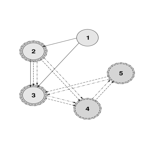
Figure 1: Union of networks $S^{k}=(I^{k},U^{k}),k\in K=\{1,2,3\}$

$$\begin{array}[]{c}x^{1}_{12}+x^{1}_{13}=4\\ x^{1}_{23}-x^{1}_{12}=6\\ -x^{1}_{13}-x^{1}_{23}=-10\\ \end{array}$$

$$\begin{array}[]{c}x^{2}_{23}+x^{2}_{24}=5\\ x^{2}_{34}-x^{2}_{23}-x^{2}_{53}=-5\\ x^{2}_{45}-x^{2}_{24}-x^{2}_{34}=1\\ x^{2}_{53}-x^{2}_{45}=-1\\ \end{array}$$ (1a)

$$\begin{array}[]{c}x^{3}_{23}+x^{3}_{24}=5\\ x^{3}_{34}-x^{3}_{23}-x^{3}_{53}=-7\\ x^{3}_{45}-x^{3}_{24}-x^{3}_{34}=1\\ x^{3}_{53}-x^{3}_{45}=1\\ \end{array}$$

$$\begin{array}[]{c}2x^{1}_{12}+3x^{1}_{13}+x^{1}_{23}+4x^{2}_{23}+2x^{3}_{23}+3x^{2}_{24}-4x^{3}_{24}+2x^{2}_{34}+x^{3}_{34}-\\ x^{2}_{45}+7x^{3}_{45}+x^{2}_{53}+2x^{3}_{53}=69\\ x^{1}_{12}+2x^{1}_{13}+2x^{1}_{23}+5x^{2}_{23}+3x^{3}_{23}-x^{2}_{24}-x^{3}_{24}+x^{2}_{34}+x^{3}_{34}-\\ 2x^{2}_{45}+3x^{3}_{45}+2x^{2}_{53}-x^{3}_{53}=58\\ \end{array}$$ (2a)

$$\begin{array}[]{c}x^{2}_{24}+x^{3}_{24}=1\\ \end{array}$$ (3a)

We choose a support of the network $S=(I,U)$ for the system (1a). By Theorem 2 (Network Support Criterion), we build spanning trees
$U^{k}_{T},k\in K=\{1,2,3\}$: $U^{1}_{T}=\{(1,2)^{1},(1,3)^{1}\}$, $U^{2}_{T}=\{(2,3)^{2},(2,4)^{2},(4,5)^{2}\}$, $U^{3}_{T}=\{(2,4)^{3},(3,4)^{3},(4,5)^{3}\}$.

Now, we compute the set $\{\delta^{k}(\tau,\rho),(\tau,\rho)^{k}\in U^{k}\setminus U^{k}_{T}\}$ of characteristic vectors with respect to the constructed spanning tree $U^{k}_{T},k\in K=\{1,2,3\}$.

Table 1 The set of characteristic vectors with respect to the spanning tree $U^{1}_{T}$

$(i,j)^{1}$	$(1,2)^{1}$	$(1,3)^{1}$	$(2,3)^{1}$
$\delta^{k}_{ij}(\tau,\rho)=\delta^{1}_{ij}(2,3)$	$1$	$-1$	$1$

Table 2 The set of characteristic vectors with respect to the spanning tree $U^{2}_{T}$

$(i,j)^{2}$	$(2,3)^{2}$	$(2,4)^{2}$	$(4,5)^{2}$	$(3,4)^{2}$	$(5,3)^{2}$
$\delta^{k}_{ij}(\tau,\rho)=\delta^{2}_{ij}(3,4)$	$1$	$-1$	$0$	$1$	$0$
$\delta^{k}_{ij}(\tau,\rho)=\delta^{2}_{ij}(5,3)$	$-1$	$1$	$1$	$0$	$1$

Table 3 The set of characteristic vectors with respect to the spanning tree $U^{3}_{T}$

$(i,j)^{3}$	$(2,4)^{3}$	$(3,4)^{3}$	$(4,5)^{3}$	$(2,3)^{3}$	$(5,3)^{3}$
$\delta^{k}_{ij}(\tau,\rho)=\delta^{3}_{ij}(2,3)$	$-1$	$1$	$0$	$1$	$0$
$\delta^{k}_{ij}(\tau,\rho)=\delta^{3}_{ij}(5,3)$	$0$	$1$	$1$	$0$	$1$

Let’s compute the partial solution of the system (1a) for each $k\in K=\{1,2,3\}$ according to the Remark 2: $\tilde{x}^{1}=(\tilde{x}^{1}_{12},\tilde{x}^{1}_{13},\tilde{x}^{1}_{23})^{T}=(-6,10,0)^{T}$, $\tilde{x}^{2}=(\tilde{x}^{2}_{23},\tilde{x}^{2}_{24},\tilde{x}^{2}_{45},\tilde{x}^{2}_{34},\tilde{x}^{2}_{53})^{T}=(5,0,1,0,0)^{T}$, $\tilde{x}^{3}=(\tilde{x}^{3}_{24},\tilde{x}^{3}_{34},\tilde{x}^{3}_{45},\tilde{x}^{3}_{23},\tilde{x}^{3}_{53})^{T}=(5,-7,-1,0,0)^{T}.$

We form the set $U_{C}=\displaystyle\bigcup^{3}_{k=1}U^{k}_{C}=\{(2,3)^{1},(3,4)^{2},(2,3)^{3}\}$ of cyclic arcs. The remaining arcs will be included into the set $U_{N}=\displaystyle\bigcup^{3}_{k=1}U^{k}_{N}=\{(5,3)^{2},(5,3)^{3}\}$. Structures, representing the union of the sets $U^{k}_{T}\bigcup U^{k}_{C},k\in K=\{1,2,3\}$ are shown on Figure 2.

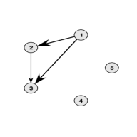
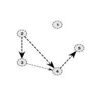
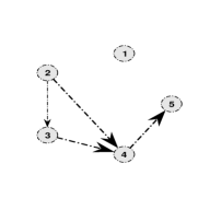
Figure 2: Sets $U^{k}_{T}\bigcup U^{k}_{C}$ for networks $S^{k},k\in K=\{1,2,3\}$

Using formula (18) we compute the determinants of the cycles $L^{k}_{\tau\rho}$, entailed by the arcs $(\tau,\rho)^{k}\in U^{k}\backslash U^{k}_{T}$, for each $k\in K=\{1,2,3\}$, with respect to the equation (2a) with the number $p=1,2$ (Table 4).

Table 4 Determinants of the cycles $L^{k}_{\tau\rho}$, entailed by the arcs $(\tau,\rho)^{k}\in U^{k}\backslash U^{k}_{T},k\in K=\{1,2,3\}$

$(\tau,\rho)^{k}$	$(2,3)^{1}$	$(3,4)^{2}$	$(5,3)^{2}$	$(2,3)^{3}$	$(5,3)^{3}$
$R_{1}(L^{k}_{\tau\rho})$	$0$	$3$	$-1$	$7$	$10$
$R_{2}(L^{k}_{\tau\rho})$	$1$	$7$	$-6$	$5$	$3$

Now, let’s compute the values $\delta_{ij}(L^{k}_{\tau\rho}),(i,j)\in U_{0},(\tau,\rho)^{k}\in U^{k}\setminus U^{k}_{T},k\in K=\{1,2,3\}$ according to the formula (24) for the example (1a)-(3a), $U_{0}=\{(2,4)\}$, $K_{0}(2,4)=\{2,3\}$ (Table 5).

Table 5 The values $\delta_{ij}(L^{k}_{\tau\rho}),(i,j)\in U_{0},(\tau,\rho)^{k}\in U^{k}\setminus U^{k}_{T},k\in K=\{1,2,3\}$

$(\tau,\rho)^{k}$	$(2,3)^{1}$	$(3,4)^{2}$	$(5,3)^{2}$	$(2,3)^{3}$	$(5,3)^{3}$
$\delta_{24}(L^{k}_{\tau\rho})$	$0$	$-1$	$1$	$-1$	$0$

Before assembling the matrix $D$ of the system (28), let’s number the arcs of the set : $U_{C}=\{(2,3)^{1},(3,4)^{2},(2,3)^{3}\}:t(2,3)^{1}=1,\,t(3,4)^{2}=2,\,t(2,3)^{3}=3$. The numbering within the set $U_{0}=\{(2,4)\}$ is trivial: $\xi(2,4)=1$.

First, we construct the matrix $D_{1}=(R_{p}(L^{k}_{\tau\rho}),\,p=\overline{1,2},\,t(\tau,\rho)^{k}=\overline{1,3})$ of the determinants of the cycles $L^{k}_{\tau\rho}$ , entailed by the arcs $(\tau,\rho)^{k}\in U_{C}$, by selecting the corresponding columns from the Table 4:

$$D_{1}=\left(\begin{array}[]{ccc}0&3&7\\ 1&7&5\end{array}\right).$$

Similarly, by selecting the corresponding columns from the Table 5, we form the matrix $D_{2}=(\delta_{24}(L^{k}_{\tau\rho}),\,\xi(2,4)=1,\,t(\tau,\rho)^{k}=\overline{1,3})$:

$$D_{2}=(0\quad-1\quad-1).$$

Thus, joining $D_{1}$ and $D_{2}$ together, we obtain the matrix of the system (28):

$$D=\left(\begin{array}[]{ccc}0&3&7\\ 1&7&5\\ 0&-1&-1\end{array}\right),\mbox{det}D\neq 0.$$

Let us compute the vector $\beta$ in the right hand side of (28) using formulae (29):

$$\beta_{1}=A^{1}-R_{1}(L^{2}_{53})x^{2}_{53}-R_{1}(L^{3}_{53})x^{3}_{53},$$

$$\beta_{2}=A^{2}-R_{2}(L^{2}_{53})x^{2}_{53}-R_{2}(L^{3}_{53})x^{3}_{53},$$

$$\beta_{3}=A_{24}-\delta_{24}(L^{2}_{53})x^{2}_{53}-\delta_{24}(L^{3}_{53})x^{3}_{53}.$$

The values $R_{p}(L^{2}_{53})$, $R_{p}(L^{3}_{53})$, $p=1,2$ of the determinants of the cycles $L^{k}_{\tau\rho}$, entailed by the arcs $(\tau,\rho)^{k}\in U_{N}$, as well as the values $\delta_{24}(L^{2}_{53})$ and $\delta_{24}(L^{3}_{53})$, are already computed and stored within the Table 4 and Table 5. The numbers $A^{1},A^{2},A_{24}$ are evaluated using the formulae (19) and (26):

$$A^{1}=\alpha_{1}-\lambda_{12}^{11}\tilde{x}^{1}_{12}-\lambda_{13}^{11}\tilde{x}^{1}_{13}-\lambda_{23}^{21}\tilde{x}^{2}_{23}-\lambda_{24}^{21}\tilde{x}^{2}_{24}-\lambda_{45}^{21}\tilde{x}^{2}_{45}-\lambda_{24}^{31}\tilde{x}^{3}_{24}-\lambda_{34}^{31}\tilde{x}^{3}_{34}-\lambda_{45}^{31}\tilde{x}^{3}_{45}=66,$$

$$A^{2}=\alpha_{2}-\lambda_{12}^{12}\tilde{x}^{1}_{12}-\lambda_{13}^{12}\tilde{x}^{1}_{13}-\lambda_{23}^{22}\tilde{x}^{2}_{23}-\lambda_{24}^{22}\tilde{x}^{2}_{24}-\lambda_{45}^{22}\tilde{x}^{2}_{45}-\lambda_{24}^{32}\tilde{x}^{3}_{24}-\lambda_{34}^{32}\tilde{x}^{3}_{34}-\lambda_{45}^{32}\tilde{x}^{3}_{45}=36,$$

$$A_{24}=z_{24}-\tilde{x}^{2}_{24}-\tilde{x}^{3}_{24}=-4.$$

Thus, we have defined the vector $\beta=\left(\begin{array}[]{c}66+x^{2}_{53}-10x^{3}_{53}\\ 36+6x^{2}_{53}-3x^{3}_{53}\\ -4-x^{2}_{53}\end{array}\right).$

Since the matrix $D$ turned out to be non-singular, we can use formula (30) for finding the solution $x_{C}=(x^{k}_{\tau\rho},(\tau,\rho)^{k}\in U_{C}^{k},k\in K)$ of the system (28):

$$\left(\begin{array}[]{c}x^{1}_{23}\\ x^{2}_{34}\\ x^{3}_{23}\\ \end{array}\right)=\left(\begin{array}[]{rcr}\displaystyle\frac{1}{2}&1&\displaystyle\frac{17}{2}\\ -\displaystyle\frac{1}{4}&0&-\displaystyle\frac{7}{4}\\ \displaystyle\frac{1}{4}&0&\displaystyle\frac{3}{4}\\ \end{array}\right)\left(\begin{array}[]{c}66+x^{2}_{53}-10x^{3}_{53}\\ 36+6x^{2}_{53}-3x^{3}_{53}\\ -4-x^{2}_{53}\\ \end{array}\right).$$

Finally, using formulae (31) - (32), we can define the solution of the system (1a)-(3a) with $x^{2}_{53},x^{3}_{53}$, being independent variables:

$$x^{1}_{23}=35-2x^{2}_{53}-8x^{3}_{53},x^{2}_{34}=-\frac{19}{2}+\frac{3}{2}x^{2}_{53}+\frac{5}{2}x^{3}_{53},x^{3}_{23}=\frac{27}{2}-\frac{1}{2}x^{2}_{53}-\frac{5}{2}x^{3}_{53},$$

$$x^{1}_{12}=29-2x^{2}_{53}-8x^{3}_{53},$$

$$x^{1}_{13}=-25+2x^{2}_{53}+8x^{3}_{53},$$

$$x^{2}_{23}=-\frac{9}{2}+\frac{1}{2}x^{2}_{53}+\frac{5}{2}x^{3}_{53},$$

$$x^{2}_{24}=\frac{19}{2}-\frac{1}{2}x^{2}_{53}-\frac{5}{2}x^{3}_{53},$$

$$x^{2}_{45}=x^{2}_{53}+1,$$

$$x^{3}_{24}=-\frac{17}{2}+\frac{1}{2}x^{2}_{53}+\frac{5}{2}x^{3}_{53},$$

$$x^{3}_{34}=\frac{13}{2}-\frac{1}{2}x^{2}_{53}-\frac{3}{2}x^{3}_{53},$$

$$x^{3}_{45}=x^{3}_{53}-1,$$

$$x^{2}_{53},x^{3}_{53}\in\mathbf{R}.$$

L.A. Pilipchuk	E.S. Vecharynski
Belarus State University	University of Colorado Denver
Department of Applied Mathematics	Department of Mathematical Sciences
and Computer Science	Campus Box 170
Nezalezhnasci Ave. 4	P.O. Box 173364
Minsk	Denver, CO 80217-3364 USA
220050 Belarus	e-mail:
e-mail: pilipchuk@bsu.by	Yaugen.Vecharynski@ucdenver.edu

References

[1]
Ravindra K. Ahuja, Thomas L. Magnanti, James B. Orlin.: Network
Flows: Theory, Algorithms, and Applications. New Jersey, 1993.
[2]
Gabasov R., Kirillova F. M., Kostjukova O. I.: Constructive methods of
optimization. Part 3. Network flow problems (in Russian). Universitetskoje, Minsk,
1986.
[3]
Gabasov R., Kirillova F. M.:
Methods of linear programming. Part 3. Special problems (in
Russian). BGU, Minsk, 1980.
[4]
Pilipchuk L. A., Malakhouskaya Y.V., Kincaid D. R., Lai M.:
Algorithms of Solving Large Sparse Underdetermined Linear Systems
with Embedded Network Structure. East-West J. of Mathematics. Vol.
4, N∘2. p.191202(2002).
[5]
Pilipchuk L. A.: Network optimization problems. Applications of
Mathematics in Engineering and Economics. Eds. D. Ivanchev and
M.D. Todorov. Heron Press, Sofia(2002).
[6]
Pilipchuk L.A., Gutkovsky V.V.: Inhomogeneous multinetwork
dynamic problem. 16 th IMACS World Congress on Scientific
Computation, Applied Mathematics and Simulation. Lausanne -
Switzerland(2000).
[7]
Pilipchuk L.A., Koliago Yu. L., Pesheva Yu. H.: Algorithms for
Solving Large Sparse Underdetermined Linear Systems in the
Production-transport Problem with Additional Constraints.
Application of Mathematics in Engineering and Economics.
Proceedings of the 29 th International Summer School. Bulvest,
Sofia, p.229 - 233(2004).
[8]
Pilipchuk L.A.: Optimization of non-homogeneous network flows.
Information systems and technologies. Materials for 2nd
International Conference IST’2004. Minsk. Ch. 2, p.208 -
213(2004).