Probing the thermal atoms of a Bose gas through Raman transition

Abstract

We explore the many body physics of a Bose condensed atom gas at finite temperature through the Raman transition between two hyperfine levels. Unlike the Bragg scattering where the phonon-like nature of the collective excitations has been observed, a different branch of thermal atom excitation is found theoretically in the Raman scattering. This excitation is predicted in the generalized random phase approximation (GRPA) and has a gapped and parabolic dispersion relation. The gap energy results from the exchange interaction and is released during the Raman transition. The scattering rate is determined versus the transition frequency $\omega$ and the transferred momentum $\mathbf{q}$ and shows the corresponding resonance around this gap. Nevertheless, the Raman scattering process is attenuated by the superfluid part of the gas. The macroscopic wave function of the condensate deforms its shape in order to screen locally the external potential displayed by the Raman light beams. This screening is total for a condensed atom transition in order to prevent the condensate from incoherent scattering. The experimental observation of this result would explain some of the reasons why a superfluid condensate moves coherently without any friction with its surrounding.

I Introduction

Among the various approximations existing in the literature to describe a diluted Bose condensed gas at finite temperature, the generalized random phase approximation (GRPA) has been the subject of several studies Reidl ; Zhang ; condenson ; Levitov ; gap . This approximation has attracted a special attention since it is the only one in the literature with two important properties: 1) in agreement with the Hugenholtz-Pines theorem HM ; HP ; Ketterle ; Stringari , it predicts the observed gapless and phonon-like excitations; 2) the mass, momentum and energy conservation laws are fulfilled in the gas dynamical description. An approximation that satisfies these properties is said to be gapless and conserving Reidl ; HM .

Besides these unique features, the GRPA predicts also other phenomena, namely a second branch of excitations and the dynamical screening of the interaction potential. These phenomena appear also in the case of a gas of charged particles or plasma. The possibility of a second kind of excitation has been explained quite extensively in condenson ; Levitov ; gap . There is a distinction between the single particle excitations and the collective excitations. In the case of a plasma, the first corresponds to the electrically charged excitations and its dispersion relation is obtained from the pole of the one particle Green function. The second corresponds to the plasmon which is a chargeless excitation whose the dispersion relation is obtained from the pole of the susceptibility function. The plasmon mediates the interaction between two charged excitations. More precisely, during the interaction, one charged excitation emits a virtual plasmon which is subsequently reabsorbed by another charged excitation (see Fig.1).

Figure 1: Feymann diagram illustrating the mediation process: 1) For a plasma two charged excitations of momentum $\mathbf{k}$ and $\mathbf{k}^{\prime}$ mediate their interaction via a plasmon of momentum $\mathbf{q}$; 2) For a Bose gas, two excitations with one atom number unit mediate their interaction via a phonon-like collective excitation.

Remarkably, such a description holds also for a Bose gas with single atom excitations carrying one unit of atom number and with gapless collective excitations with no atom number. The poles of the Green functions have a similar structure above the critical point. But below this critical point, the existence of a macroscopic condensed fraction hybridizes the collective and single particle excitations so that the poles of the one particle Green function and the susceptibility function mix to form common branches of collective excitations gap ; HM . Thus, at the difference of a plasma, the presence of a condensed fraction prevents the direct observation of the atom-like excitation through the one particle Green function.

The dynamical screening effect predicted in the GRPA appears much more spectacular in a Bose gas. The screening effect of the coulombian interaction is well known to explain the dissociation of salt diluted in water into its ions (see Fig.2a). But it also provides an explanation to the superfluidity phenomenon i.e. the possibility of a metastable motion without any friction.

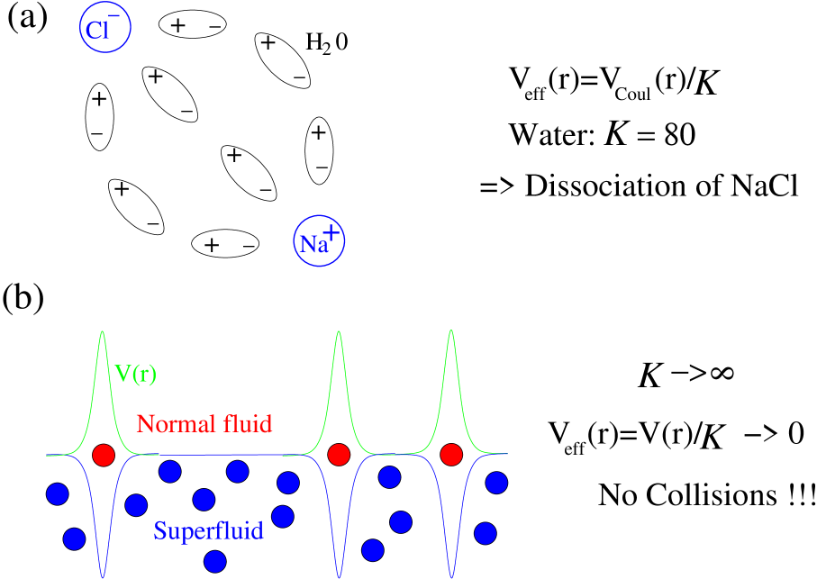
Figure 2: Illustration of the screening effect: (a) In water, the interaction force between the ions $Na^{+}$ and $Cl^{-}$ of the salt is screened by the presence of water molecules and the coulombian potential $V_{Coul}(\mathbf{r})$ is reduced by the relative permittivity factor ${\cal{K}}\sim 80$. (b) In a Bose condensed gas, a similar effect occurs. The condensed and thermal atoms represented in blue and red respectively correspond in good approximation to the superfluid and normal fluid. The interaction potential $V(\mathbf{r})$ displayed by these thermal atoms on condensed atoms are pictured qualitatively by the green line. The macroscopic wave function associated to the condensed atoms deforms its shape in order to locally modify the superfluid mean field interaction energy represented by the blue line. The net result is a total screening of the interaction potential by this mean field energy, which prevents binary collision processes between condensed and thermal atoms. In this way, one can explain qualitatively the metastability of a relative motion between the superfluid and the normal fluid.

Most of the literature on superfluidity is usually devoted to the study of metastable motion in a toroidal geometry like, for example, an annular region between two concentric cylinders possibly in rotation books ; Leggett2 . In this simply connected geometry, the angular momentum about the axis of the cylinder of the superfluid is quantized in unit of $\hbar$. The metastability of the motion is explained by the impossibility to go continuously from one quantized state to another due to the difficulty to surmount an enormous free-energy barrier. This is not the situation we want to address in this paper. We are rather focusing on the explanation of the superfluid ability to flow without any apparent friction with its surrounding.

The Landau criterion is a necessary but not sufficient condition for superfluidity. It tells about the kinematic conditions under which an external object can move relatively to a superfluid without damping its relative velocity by emitting a phonon-like collective excitation. For a dilute Bose gas at low temperature, it amounts to saying that this relative velocity must be lower than the sound velocity Stringari . The external object is assumed to be macroscopic and can be an impurity Chikkatur , an obstacle like a lattice Cataliotti or even the normal fluid condenson . In particular, this criterion does not taken into account the fact that the normal fluid is microscopically composed of thermal excitations. In a Bose condensed gas, even though their relative velocity is on average lower than the critical one, many of these excitations are very energetic with a relative velocity high enough to allow the phonon emission.

In the GRPA where these excitations correspond to the thermal atoms and under the condition of the Landau criterion, such a process is forbidden as shown qualitatively from Fig.2b. The effect of an external perturbation of the condensed atoms caused for example by the thermal atoms is attenuated by the dynamical screening. This screening is total in the sense that no effective mutual binary interaction allows a collision process which would be essential for a dissipative relaxation of the superfluid motion.

The purpose of this paper is to show that these peculiar phenomena could in principle be observed in a Raman scattering process. This process induces a transition for a given frequency $\omega$ and a wavevector $\mathbf{q}$ determined from the difference of the frequencies and the wavevectors of two laser beams books . For each wavevector corresponding to the transferred momentum, one can arbitrarily tune the frequency in order to reach the resonance energy associated to the excitation. Unlike the Bragg scattering which allows the observation of the Bogoliubov phonon-like collective excitation Ketterle ; Stringari , the Raman scattering is more selective. Not only the gas is probed with a selected energy transition and transferred momentum, but the atoms are scattered into a selected second internal hyperfine level. Through a Zeeman splitter, they can be subsequently analyzed separately from unscattered atoms. According to the GRPA, the scattered thermal atoms become distinguishable from the unscattered ones and thus release the gap energy due to the exchange interaction. In a previous study gap , we showed that this gap appears as a resonance in the frequency spectrum of the atom transition rate at $\mathbf{q}\rightarrow 0$. The possibility of momentum transfer allows to analyze the influence of the screening of the external perturbation induced by the Raman light beams.

The paper is divided as follows. In section 2, we review the time-dependant Hartree-Fock (TDHF) equations for a spinor condensate and study the linear response function to an external potential which gives results equivalent to the GRPA. Sections 3 and 4 are devoted to the Bragg and Raman scatterings respectively. Section 5 ends up with the conclusions and the perspectives.

II Time-dependant Hartree-Fock approximation

We start from the time-dependant Hartree-Fock equations for describing two component spinor Bose gas Zhang ; books labeled by $a=1,2$. The atoms have a mass $m$, feel the external potential $V_{ab}(\mathbf{r},t)$ and the Hartree and Fock mean field interaction potential characterized by the coupling constants $g_{ab}=4\pi a_{ab}/m$ expressed in terms of the scattering lengths $a_{ab}$ between components $a$ and $b$ ($\hbar=1$). Note that no Fock mean field (or exchange) interaction energy appears between condensed atoms. These equations describe the time evolution of a set of spinor wave function $\psi_{a,i}(\mathbf{r},t)$ describing $N_{i}$ atoms labeled by $i$ and depending on the position $\mathbf{r}$ and on the time $t$. For the condensed mode ($i=0$), these are:

$$\left(\begin{array}[]{cc}i{\partial_{t}}+\frac{\nabla^{2}_{\mathbf{r}}}{2m}-V_{11}&V_{12}^{*}\\ V_{12}&i{\partial_{t}}+\frac{\nabla^{2}_{\mathbf{r}}}{2m}-V_{22}\end{array}\right)\left(\begin{array}[]{c}\psi_{1,0}\\ \psi_{2,0}\end{array}\right)=$$ (5)

$$\left(\begin{array}[]{cc}\sum_{j}(g_{11}(2-\delta_{0,j})|\psi_{1,j}|^{2}+g_{12}|\psi_{2,j}|^{2})N_{j}&g_{12}\sum_{j}(1-\delta_{0,j})N_{j}\psi_{2,j}^{*}\psi_{1,j}\\ g_{12}\sum_{j}(1-\delta_{0,j})N_{j}\psi_{1,j}^{*}\psi_{2,j}&\sum_{j}(g_{22}(2-\delta_{0,j})|\psi_{2,j}|^{2}+g_{12}|\psi_{1,j}|^{2})N_{j}\end{array}\right)\left(\begin{array}[]{c}\psi_{1,0}\\ \psi_{2,0}\end{array}\right)$$ (10)

For a non condensed mode ($i\not=0$), these are

$$\left(\begin{array}[]{cc}i{\partial_{t}}+\frac{\nabla^{2}_{\mathbf{r}}}{2m}-V_{11}&V_{12}^{*}\\ V_{12}&i{\partial_{t}}+\frac{\nabla^{2}_{\mathbf{r}}}{2m}-V_{22}\end{array}\right)\left(\begin{array}[]{c}\psi_{1,i}\\ \psi_{2,i}\end{array}\right)=$$ (15)

$$\left(\begin{array}[]{cc}\sum_{j}(2g_{11}|\psi_{1,j}|^{2}+g_{12}|\psi_{2,j}|^{2})N_{j}&g_{12}\sum_{j}N_{j}\psi_{2,j}^{*}\psi_{1,j}\\ g_{12}\sum_{j}N_{j}\psi_{1,j}^{*}\psi_{2,j}&\sum_{j}(2g_{22}|\psi_{2,j}|^{2}+g_{12}|\psi_{1,j}|^{2})N_{j}\end{array}\right)\left(\begin{array}[]{c}\psi_{1,i}\\ \psi_{2,i}\end{array}\right)$$ (20)

The non condensed spinors remain orthogonal during their time evolution in the thermodynamic limit. In general, the spinor associated to the condensed mode does not remain orthogonal with the others. But according to Huse , the non orthogonality is not important in the thermodynamic limit for smooth external potential. Another way of justifying the non orthogonality is to start from an ansatz where the condensed spinor mode is described in terms of a coherent state and the non condensed ones in terms of a complete set of orthogonal Fock states i.e. $|\Psi\rangle\sim\exp(\sum_{j\not=0}b_{j}c_{j}^{\dagger}-c.c.)\prod_{i\not=0}(c_{i}^{\dagger})^{N_{i}}|0\rangle$ where $c_{i}^{\dagger}$ is the atom creation operator in the mode $i$ and $b_{j}=\sqrt{N_{0}}\sum_{a}\int d^{3}\mathbf{r}\psi^{*}_{a,j}\psi_{a,0}$. The theory remains conserving because the conservation laws are preserved on average but becomes non number conserving since the quantum state is not an eigenstate of the total particle number operator. This procedure is justified in the thermodynamic limit since the total particle number fluctuations are relatively small during the time evolution. In contrast, instead of using spinor wavefunctions, the alternative method based on the use of excitation operators is number conserving condenson ; Levitov .

The atom number $N_{i}$ for each mode is supposed time-independent in the TDHF. Strictly speaking, a collision term must be added in order to allow population transfers between the various modes. These equations are valid in the collisionless regime i.e. on a time scale shorter than the average time between two collisions $\tau\sim 1/(\sigma_{ab}nv_{T})$ where $v_{T}=\sqrt{1/\beta m}$ is the average velocity and $\sigma_{ab}=8\pi a_{ab}^{2}$ is the scattering cross section. In these conditions, the resulting frequency spectrum has a resolution limited by $\Delta\omega\sim 1/\tau$. The magnitude order of resolution of interest is given by the $g_{ab}n$’s so we require $\Delta\omega/g_{ab}n\sim\sqrt{a^{3}_{ab}n/\beta g_{ab}n}\ll 1$ which is generally the case when $a^{3}_{ab}n\ll 1$. These conditions are fulfilled for the parameter values considered in this work.

In the following, we will restrict our analysis to a bulk gas embedded in a volume $V$. At $t<0$, we assume all atoms in thermodynamic equilibrium in the level $1$ and that $V_{ab}=0$ except for $V_{22}=\omega_{0}$ which is constant and fixes the energy shift between the two sub-levels. In that case, the solutions of the TDHF are orthogonal plane waves with $i$ corresponding to the momentum $\mathbf{k}$:

$$\left(\begin{array}[]{c}\psi^{(0)}_{1,\mathbf{k}}\\ \psi^{(0)}_{2,\mathbf{k}}\end{array}\right)=\frac{\exp[i(\mathbf{k}.\mathbf{r}-\epsilon^{HF}_{1,\mathbf{k}}t)]}{\sqrt{V}}\left(\begin{array}[]{c}1\\ 0\end{array}\right)$$ (25)

where we define the Hartree-Fock energy for atoms with momentum $\mathbf{k}$:

$$\epsilon^{HF}_{1,\mathbf{k}}=\epsilon_{\mathbf{k}}+g_{11}(2n-n_{\mathbf{0}}\delta_{\mathbf{k},\mathbf{0}})$$ (26)

where $\epsilon_{\mathbf{k}}=\mathbf{k}^{2}/2m$ and where the condensed and total particle densities are $n_{\mathbf{0}}=N_{\mathbf{0}}/V$ and $n=\sum_{\mathbf{k}}N_{\mathbf{k}}/V$. Eq.(26) corresponds to the dispersion relation of the single particle excitation. At equilibrium,

$$N^{\prime}_{\mathbf{k}}=N_{\mathbf{k}}(1-\delta_{\mathbf{k},\mathbf{0}})=1/(\exp[\beta(\epsilon^{HF}_{1,\mathbf{k}}-\mu)]-1)$$ (27)

is the Bose-Einstein distribution. Below the condensation point, the chemical potential becomes $\mu=\epsilon_{\mathbf{0}}=g_{11}(2n-n_{\mathbf{0}})$ and the macroscopic occupation $N_{\mathbf{0}}$ is fixed to satisfy the total number conservation.

For $t\geq 0$, we apply an external potential. For the Bragg and Raman scatterings, these are respectively:

$$V_{11}=V_{B}\cos(\mathbf{q}.\mathbf{r}-\omega t)$$ (28)

$$V_{12}=V_{R}\exp[i(\mathbf{q}.\mathbf{r}-\omega t)]$$ (29)

We solve the system through a perturbative expansion:

$$\left(\begin{array}[]{c}\psi_{1,\mathbf{k}}\\ \psi_{2,\mathbf{k}}\end{array}\right)=\left(\begin{array}[]{c}e^{i(\mathbf{k}.\mathbf{r}-\epsilon^{HF}_{1,\mathbf{k}}t)}/\sqrt{V}+\psi^{(1)}_{1,\mathbf{k}}(\mathbf{r},t)+\psi^{(2)}_{1,\mathbf{k}}(\mathbf{r},t)\\ \psi^{(1)}_{2,\mathbf{k}}(\mathbf{r},t)\end{array}\right)$$ (34)

The equations of motion for the first order corrections are for the case of Bragg and Raman scatterings respectively:

$$\!\!\left[i{\partial_{t}}+\frac{\nabla^{2}_{\mathbf{r}}}{2m}-g_{11}(2n-\delta_{\mathbf{k},\mathbf{0}}n_{\mathbf{0}})\right]\psi^{(1)}_{1,\mathbf{k}}=$$

$$\left[V_{11}+\!\sum_{\mathbf{k^{\prime}}}g_{11}(2-\delta_{\mathbf{k^{\prime}},\mathbf{0}}\delta_{\mathbf{k},\mathbf{0}})({\psi^{(0)*}_{1,\mathbf{k^{\prime}}}}\psi_{1,\mathbf{k^{\prime}}}^{(1)}+c.c.)N_{\mathbf{k^{\prime}}}\right]\!\psi^{(0)}_{1,\mathbf{k}}$$ (35)

$$\left[i{\partial_{t}}+\frac{\nabla^{2}_{\mathbf{r}}}{2m}-\omega_{0}-g_{12}(n-\delta_{\mathbf{k},\mathbf{0}}n_{\mathbf{0}})\right]\psi^{(1)}_{2,\mathbf{k}}=\left[V_{12}+g_{12}\sum_{\mathbf{k^{\prime}}}N_{\mathbf{k^{\prime}}}{\psi^{(0)*}_{1,\mathbf{k^{\prime}}}}\psi^{(1)}_{2,\mathbf{k^{\prime}}}\right]\psi^{(0)}_{1,\mathbf{k}}$$ (36)

These two set of integral equations can be solved exactly using the methods developed in condenson . Defining the Fourier transforms:

$$V_{ab,\mathbf{q},\omega}=\int_{V}\!\!\!d^{3}\mathbf{r}\int_{0}^{\infty}\!\!\!dt\,e^{i[(\omega+i0)t-\mathbf{q}.\mathbf{r}]}V_{ab}(\mathbf{r},t)$$ (37)

one obtains in the level 1 for the condensed mode:

$$\psi^{(1)}_{1,\mathbf{0}}(\mathbf{r},t)=\sum_{\mathbf{q^{\prime}}}\int_{-\infty}^{\infty}\frac{d\omega^{\prime}}{2\pi i}\frac{e^{i(\mathbf{q^{\prime}}.\mathbf{r}-\omega^{\prime}t)}V_{11,\mathbf{q^{\prime}},\omega^{\prime}}\psi^{(0)}_{1,\mathbf{0}}(\mathbf{r},t)}{{\tilde{\cal K}}(\mathbf{q^{\prime}},\omega^{\prime})(\omega^{\prime}+i0-\epsilon_{\mathbf{q^{\prime}}})}$$ (38)

for the non condensed modes ($\mathbf{k}\not=0$):

$$\psi^{(1)}_{1,\mathbf{k}}(\mathbf{r},t)=\sum_{\mathbf{q^{\prime}}}\int_{-\infty}^{\infty}\frac{d\omega^{\prime}}{2\pi i}\frac{e^{i(\mathbf{q^{\prime}}.\mathbf{r}-\omega^{\prime}t)}V_{11,\mathbf{q^{\prime}},\omega^{\prime}}\psi^{(0)}_{1,\mathbf{k}}(\mathbf{r},t)}{{\cal K}(\mathbf{q^{\prime}},\omega^{\prime})(\omega^{\prime}+i0-\epsilon_{\mathbf{k}+\mathbf{q^{\prime}}}+\epsilon_{\mathbf{k}})}$$ (39)

and in the level 2 for all modes:

$$\psi^{(1)}_{2,\mathbf{k}}(\mathbf{r},t)=\sum_{\mathbf{q^{\prime}}}\int_{-\infty}^{\infty}\frac{d\omega^{\prime}}{2\pi i}\times$$ (40)

$$\displaystyle\frac{e^{i(\mathbf{q^{\prime}}.\mathbf{r}-\omega^{\prime}t)}V_{12,\mathbf{q^{\prime}},\omega^{\prime}}\psi^{(0)}_{1,\mathbf{k}}(\mathbf{r},t)}{{\cal K}_{12}(\mathbf{q^{\prime}},\omega^{\prime})(\omega^{\prime}+i0-\omega_{0}-\epsilon_{\mathbf{k}+\mathbf{q^{\prime}}}+\epsilon_{\mathbf{k}}+(2g_{11}-g_{12})n+\delta_{\mathbf{k},\mathbf{0}}(g_{12}-g_{11})n_{\mathbf{0}})}$$

These formulae resemble the one obtained from the non interacting Bose gas excepted for the mean field term in (40) and the extra factors representing the screening effect. For the Bragg scattering, these factors can be written as condenson :

$${\tilde{\cal K}}(\mathbf{q},\omega)=\frac{\Delta(\mathbf{q},\omega)}{(\omega+i0)^{2}-\epsilon_{\mathbf{q}}^{2}}$$ (41)

$${{\cal K}}(\mathbf{q},\omega)=\frac{\Delta(\mathbf{q},\omega)}{(\omega+i0)^{2}-\epsilon_{\mathbf{q}}^{2}+2g_{11}n_{\mathbf{0}}\epsilon_{\mathbf{q}}}$$ (42)

where

$$\Delta(\mathbf{q},\omega)=(1-2g_{11}\chi_{0}(\mathbf{q},\omega))[(\omega+i0)^{2}-{\epsilon^{B}_{\mathbf{q}}}^{2}]-8g_{11}\chi_{0}(\mathbf{q},\omega)g_{11}n_{\mathbf{0}}\epsilon_{\mathbf{q}}$$ (43)

is the propagator for the collective excitations, $\epsilon^{B}_{\mathbf{q}}=\sqrt{c^{2}\mathbf{q}^{2}+\epsilon_{\mathbf{q}}^{2}}$ is the Bogoliubov excitation energy, $c=\sqrt{g_{11}n_{\mathbf{0}}/m}$ is the sound velocity and

$$\chi_{0}(\mathbf{q},\omega)=\frac{1}{V}\sum_{\mathbf{k}}\frac{N^{\prime}_{\mathbf{k}}-N^{\prime}_{\mathbf{k}+\mathbf{q}}}{\omega+i0+\epsilon_{\mathbf{k}}-\epsilon_{\mathbf{k+q}}}$$ (44)

is the susceptibility function describing the normal atoms. For the Raman scattering, it is

$${{\cal K}}_{12}(\mathbf{q},\omega)=1-g_{12}\chi_{0,12}(\mathbf{q},\omega)$$ (45)

where

$$\chi_{0,12}(\mathbf{q},\omega)=\frac{1}{V}\sum_{\mathbf{k}}\frac{N_{\mathbf{k}}}{\omega+i0-\omega_{0}+\epsilon_{\mathbf{k}}-\epsilon_{\mathbf{k+q}}+(2g_{11}-g_{12})n+\delta_{\mathbf{k},\mathbf{0}}(g_{12}-g_{11})n_{\mathbf{0}}}$$ (46)

Knowing the Fourier transform of the potential $V_{11,\mathbf{q^{\prime}},\omega^{\prime}}=\sum_{\pm}iV_{B}\delta_{\mathbf{q^{\prime}},\pm\mathbf{q}}/2(\omega^{\prime}+i0\mp\omega)$ and $V_{12,\mathbf{q^{\prime}},\omega^{\prime}}=iV_{R}\delta_{\mathbf{q},\mathbf{q^{\prime}}}/(\omega^{\prime}+i0-\omega)$, Eqs.(38,39,40) are calculated using the contour integration method over $\omega^{\prime}$ by analytic continuation in the lower half plane. As a consequence, the poles of the integrand tell about the excitation frequencies induced by the external perturbation. The pole of the propagator containing $\mathbf{k}$ corresponds to atom excitation involving one mode only while the poles coming from the screening factors correspond to the excitations involving all modes $\mathbf{k}$ collectively. Thus, the TDHF approach predicts both single atom and collective excitations. Note that the single mode excitation is not possible for the condensed atoms since the corresponding pole is compensated by a zero coming from the screening factor. The expressions (38,39,40) have an interpretation shown in Fig.3. An atom of momentum $\mathbf{k}$ is scattered into a state of momentum $\mathbf{k+q^{\prime}}$ by means of an external interaction mediated by a virtual collective excitation of momentum $\mathbf{q^{\prime}}$.

Figure 3: Diagrammatic representation of the scattering of an atom by an external potential

III Bragg scattering

Let us first review the Bragg scattering process . Up to the second order in the Bragg potential, the atoms number for any mode $\mathbf{k}$ can be decomposed into an unscattered part:

$$N_{\mathbf{k}}^{unscat}=N_{\mathbf{k}}\left[1+\int_{V}d^{3}\mathbf{r}(\psi^{(0)*}_{1,\mathbf{k}}\psi^{(2)}_{1,\mathbf{k}}+c.c.)\right]$$ (47)

and a scattered part:

$$N_{\mathbf{k}}^{scat}=N_{\mathbf{k}}\int_{V}d^{3}\mathbf{r}|\psi^{(1)}_{1,\mathbf{k}}|^{2}$$ (48)

Instead of evaluating the second order term, $N_{\mathbf{k}}^{unscat}$ is determined through the conservation relation $N_{\mathbf{k}}=N_{\mathbf{k}}^{unscat}+N_{\mathbf{k}}^{scat}$. Generally speaking within the sublevel 1, the scattered atoms cannot be distinguished from the unscattered ones. But in order to understand the underlying physics, we assume that distinction is possible. Within the second order perturbation theory, the quantity of interest is the scattered atom rate per unit of time and is expected to reach a stationary value after a certain transition time. In the following, we shall analyze these transition rates for time long enough that transient effects disappear. In these conditions, a perturbative approach is still valid for very large time provided that the scattered atom number remains low compared to unscattered ones. This last requirement is always satisfied with a sufficiently weak external perturbation.

At zero temperature, only the condensed wave function is modified and Eq.(38) becomes after contour integration over $\omega^{\prime}$:

$$\psi^{(1)}_{1,\mathbf{0}}(\mathbf{r},t)=\frac{V_{B}}{2i}\psi^{(0)}_{1,\mathbf{0}}(\mathbf{r},t)\sum_{\pm}e^{\pm i\mathbf{q}.\mathbf{r}}\!\!\left[\frac{(e^{-i\epsilon^{B}_{\mathbf{q}}t}-e^{\mp i\omega t})(\epsilon^{B}_{\mathbf{q}}+\epsilon_{\mathbf{q}})}{2\epsilon^{B}_{\mathbf{q}}(\epsilon^{B}_{\mathbf{q}}\mp\omega)}+\frac{(e^{i\epsilon^{B}_{\mathbf{q}}t}-e^{\mp i\omega t})(\epsilon_{\mathbf{q}}-\epsilon^{B}_{\mathbf{q}})}{2\epsilon^{B}_{\mathbf{q}}(\epsilon^{B}_{\mathbf{q}}\pm\omega)}\right]$$ (49)

The response function is only resonant at the Bogoliubov energy $\pm\epsilon_{\mathbf{q}}^{B}$. Also no transient response appears at zero temperature. Using (38) and (39), the total number of scattered atom can be obtained by determining the total momentum:

$$\mathbf{P}=\sum_{\mathbf{k}}N_{\mathbf{k}}\int_{V}d^{3}\mathbf{r}\,\psi^{*}_{1,\mathbf{k}}\frac{\nabla_{\mathbf{r}}}{i}\psi_{1,\mathbf{k}}=\sum_{\mathbf{k}}N_{\mathbf{k}}\int_{V}d^{3}\mathbf{r}\,|\psi^{(1)}_{1,\mathbf{k}}|^{2}\mathbf{q}$$ (50)

In the large time limit, the total momentum rate is related to the imaginary part of the susceptibility response function $\chi=\chi^{\prime}-i\chi^{\prime\prime}$ through Ketterle ; Stringari :

$$\frac{d\mathbf{P}}{dt}\stackrel{{\scriptstyle t\rightarrow\infty}}{{=}}2\mathbf{q}\left(\frac{V_{B}}{2}\right)^{2}\chi^{\prime\prime}(\mathbf{q},\omega)$$ (51)

Using Eq.(49), we recover that:

$$\chi^{\prime\prime}(\mathbf{q},\omega)=\pi S_{\mathbf{q}}N_{\mathbf{0}}(\delta(\omega-\epsilon^{B}_{\mathbf{q}})-\delta(\omega+\epsilon^{B}_{\mathbf{q}}))$$ (52)

where $S_{\mathbf{q}}=\epsilon_{\mathbf{q}}/\epsilon^{B}_{\mathbf{q}}$ is the static structure factor. The delta function comes from the relation $\delta(x)=\lim_{t\rightarrow\infty}\sin(xt)/(\pi x)$. The result (52) obtained in the GRPA is identical to the one obtained from the Bogoliubov approach where $S_{\mathbf{q}}$ can be calculated equivalently from the four points correlation function Stringari ; books . But in any case the generated phonon like excitation is still a part of the macroscopic wave function $\psi_{1,\mathbf{0}}(\mathbf{r},t)$.

At temperatures different from zero, the poles become imaginary which means that any Bogoliubov excitation is absorbed by a thermal atom excitation Reidl ; condenson . This phenomenon is known as the Landau damping. So for long time, only the residues of (38) with poles touching the real axis contribute whereas the others give rise to transient terms negligible for long time. Thus the perturbative part becomes:

$$\psi^{(1)}_{1,\mathbf{0}}(\mathbf{r},t) \stackrel{{\scriptstyle t\rightarrow\infty}}{{=}} \frac{V_{B}}{2i}\psi^{(0)}_{1,\mathbf{0}}(\mathbf{r},t)\sum_{\pm}\frac{e^{\pm i(\mathbf{q}.\mathbf{r}-\omega t)}}{{\tilde{\cal K}}(\pm\mathbf{q},\pm\omega)(\pm\omega-\epsilon_{\mathbf{q}})}$$ (53)

$$\psi^{(1)}_{1,\mathbf{k}}(\mathbf{r},t) \stackrel{{\scriptstyle t\rightarrow\infty}}{{=}} \frac{V_{B}}{2i}\psi^{(0)}_{1,\mathbf{k}}(\mathbf{r},t)\sum_{\pm}\left(\frac{e^{\mp i\omega t}}{{{\cal K}}(\pm\mathbf{q},\pm\omega)}-\frac{e^{-i(\epsilon_{\mathbf{k}\pm\mathbf{q}}-\epsilon_{\mathbf{k}})t}}{{{\cal K}}(\pm\mathbf{q},\epsilon_{\mathbf{k}\pm\mathbf{q}}-\epsilon_{\mathbf{k}})}\right)\frac{e^{\pm i\mathbf{q}.\mathbf{r}}}{(\pm\omega-\epsilon_{\mathbf{k}\pm\mathbf{q}}+\epsilon_{\mathbf{k}})}$$ (54)

Using the property $\Delta(\mathbf{q},\omega)=\Delta^{*}(-\mathbf{q},-\omega)$, the total number in the condensed mode reaches a constant value

$$N_{\mathbf{0}}^{scat}\stackrel{{\scriptstyle t\rightarrow\infty}}{{=}}\left(\frac{V_{B}}{2}\right)^{2}\frac{2(\epsilon^{2}_{\mathbf{q}}+\omega^{2})N_{\mathbf{0}}}{|\Delta(\mathbf{q},\omega)|^{2}}$$ (55)

and the scattered thermal atom rate is given by:

$$\frac{dN_{\mathbf{k}}^{scat}}{dt}\stackrel{{\scriptstyle t\rightarrow\infty}}{{=}}2\pi\left(\frac{V_{B}}{2}\right)^{2}\sum_{\pm}\frac{\delta(\pm\omega-\epsilon_{\mathbf{k}\pm\mathbf{q}}+\epsilon_{\mathbf{k}})N_{\mathbf{k}}}{|{\cal K}(\mathbf{q},\omega)|^{2}}$$ (56)

From (51), we deduce for the imaginary susceptibility:

$$\chi^{\prime\prime}(\mathbf{q},\omega)=-\frac{1}{g_{11}}{\rm Im}\left(\frac{1}{{\cal K}(\mathbf{q},\omega)}\right)$$ (57)

The basic interpretation of these formulae is the following. At finite temperature, the collective excitation modes created by the external perturbation are damped over a time given by the inverse of the Landau damping. So the number of collectively excited condensed atom reaches the constant value (55) when the produced collective excitations rate compensates their absorption rate by thermal atoms. This constant value is higher for a transition frequency and a transferred momentum close to the resonance $\omega=\epsilon_{c}\sim\pm\epsilon^{B}_{\mathbf{q}}$.

The formula (56) is a generalization of the Fermi-Golden rule when the screening effect is taken into account. The external potential perturbs the thermal atoms of momentum $\mathbf{k}$ in two channels by transferring a momentum $\pm\mathbf{q}$ and a transition energy $\pm\omega$ such that the resulting single atom excitation has a momentum $\mathbf{k}\pm\mathbf{q}$ and a kinetic energy $\epsilon_{\mathbf{k}\pm\mathbf{q}}=\epsilon_{\mathbf{k}}\pm\omega$. The presence of the screening factor amplifies or reduces the scattering rate. Amplification (or anti-screening) occurs for a frequency close to the resonance energy $\epsilon_{c}$ of the collective excitations. On the contrary, dynamical screening occurs for a frequency close to the pole of the screening factor and is total for transition involving condensed atom at $\omega=\epsilon_{\mathbf{q}}$. Thus, in GRPA, attempt to generate incoherence through single condensed atom scattering is forbidden at finite temperature. Only collective excitations affect the condensed mode but they are damped and therefore cannot contribute to effectively transfer condensed atoms to a different mode condenson . It is taught in standard textbooks books that, in the impulse approximation used for large $\mathbf{q}$, the response of the system is sensitive to the momentum distribution of the gas, since the atoms behave like independent particle. In particular, a delta peak is expected to account for the presence of a condensate fraction. The difficulty of the observation of this peak could be explained by this impossibility of a single condensed atom excitation at finite temperature. For completeness, let us mention that interaction with thermal atoms can be also totally screened and inspection of the formulae (42) shows that this happens for $\epsilon_{g}=\pm\sqrt{\epsilon_{\mathbf{q}}^{2}-c^{2}\mathbf{q}^{2}}$ Zhang . Fig. 4 shows these features in the frequency spectrum for the total momentum rate (57) at fixed $\mathbf{q}$. We choose the typical density observed experimentally for ${}^{87}Rb$ at the trap center Stringari .

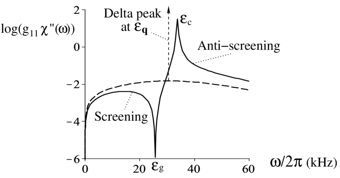
Figure 4: Imaginary susceptibility $\chi^{\prime\prime}$ of a bulk Bose condensed gas for $\epsilon_{\mathbf{q}}=2\pi\times 30{\rm kHz}$ versus the detuning frequency $\delta\omega$. The superfluid fraction is 94%, $g_{11}n=2\pi\times 4.3{\rm kHz}$, $k_{B}T/g_{11}n=2.11$ and $a_{11}^{3}n=5.6\,10^{-5}$. The black dashed/solid curve is the rate calculated in absence/presence of the screening factor. Both regimes of screening and anti-screening are displayed close to the zero $\epsilon_{g}$ and to the resonance $\epsilon_{c}$ respectively. In particular, the screening prevents the observation of a huge delta peak associated to the condensed mode.

These results can be put in direct relation with the analysis of impurity scattering Nozieres . Indeed, the dynamic response function is related to the dynamic structure factor through the fluctuation-dissipation theorem: $S(\mathbf{q},\omega)=\chi^{\prime\prime}(\mathbf{q},\omega)/\pi(1-\exp(-\beta\omega))$. The dynamic structure factor is directly connected to the transition probability rate ${\cal P}(\mathbf{q},\omega)$ that an external particle or impurity changes its initial momentum $\mathbf{p}$ and energy $E_{\mathbf{p}}$ into $\mathbf{p}+\mathbf{q}$ and $E_{\mathbf{p}+\mathbf{q}}=E_{\mathbf{p}}+\omega$ respectively:

$${\cal P}(\mathbf{q},\omega)=2\pi|{\cal{V}}_{\mathbf{q}}|^{2}S(\mathbf{q},\omega)$$ (58)

where $\cal{V}_{\mathbf{q}}$ is the Fourier transform of the interaction potential between the impurity and the atom gas. The total rate of scattering $\Gamma_{\mathbf{p}}$ results from a virtual process involving emission and absorption of the collective excitations:

$$\Gamma_{\mathbf{p}} = \sum_{\mathbf{q}}2\pi|{\cal{V}}_{\mathbf{q}}|^{2}S(\mathbf{q},E_{\mathbf{p}+\mathbf{q}}-E_{\mathbf{p}})$$ (59)

$$= \sum_{\mathbf{q},\mathbf{k}}2\pi|\frac{{\cal{V}}_{\mathbf{q}}}{{\cal{K}}(\mathbf{q},E_{\mathbf{p}+\mathbf{q}}-E_{\mathbf{p}})}|^{2}\delta(\epsilon_{\mathbf{k}}+E_{\mathbf{p}}-E_{\mathbf{p}+\mathbf{q}}-\epsilon_{\mathbf{k}-\mathbf{q}})N^{\prime}_{\mathbf{k}}(1+N^{\prime}_{\mathbf{k}-\mathbf{q}})$$ (60)

As a consequence, the impurity scattering is possible provided that the energy and momentum are conserved in a effective collision with a thermal atom of momentum $\mathbf{k}$ mediated by a virtual collective excitation. Note that total screening prevents impurity scattering involving ongoing and outgoing condensed atoms. In contrast, for temperature close to zero, the Landau damping approaches zero since $\chi_{0}(\mathbf{q},\omega)\rightarrow 0$ so that the application of Eq.(52) to (59) leads to an on-energy shell process of absorption and emission of a collective excitation. We obtain:

$$\Gamma_{\mathbf{p}} = \sum_{\pm,\mathbf{q}}2\pi|{\cal{V}}_{\mathbf{q}}|^{2}S_{\mathbf{q}}(n^{B}_{\mathbf{q}}+\delta_{\pm,+})\delta(\pm\epsilon^{B}_{\mathbf{q}}+E_{\mathbf{p}+\mathbf{q}}-E_{\mathbf{p}})$$ (61)

where $n^{B}_{\mathbf{q}}=1/(\exp(\beta\epsilon^{B}_{\mathbf{q}})-1)$. This limit case leads to the apparent interpretation of an impurity interacting with a thermal bath of phonon-like quasi-particle. This situation has been considered in Montina in the study of the impurity dynamics. Instead, Eq.(60) provides a generalization for higher temperature emphasizing that any external particle can excite a single thermal atom alone but not a condensed one.

IV Raman scattering

The conclusions so far obtained in the Bragg process can be extended straightforwardly to the case of Raman scattering with the difference that only one channel of scattering is possible. For the purpose of simplicity, we choose the case $g=g_{ab}$. Also this channel is easier to access experimentally. Defining the detuning $\delta\omega=\omega-\omega_{0}$, explicit calculations of the spinor component (40) in the second sublevel give:

$$\psi^{(1)}_{2,\mathbf{k}}(\mathbf{r},t) \stackrel{{\scriptstyle t\rightarrow\infty}}{{=}} \left(\frac{e^{-i\omega t}}{{{\cal K}}_{12}(\mathbf{q},\omega)}-\frac{e^{i(\epsilon_{\mathbf{k}}+gn-\epsilon_{\mathbf{k}+\mathbf{q}}-\omega_{0})t}}{{{\cal K}}_{12}(\mathbf{q},\omega_{0}+\epsilon_{\mathbf{k}+\mathbf{q}}-\epsilon_{\mathbf{k}}-gn)}\right)\frac{e^{i\mathbf{q}.\mathbf{r}}V_{R}\psi^{(0)}_{1,\mathbf{k}}(\mathbf{r},t)}{i(\delta\omega+\epsilon_{\mathbf{k}}+gn-\epsilon_{\mathbf{k}+\mathbf{q}})}$$ (62)

So we obtain for the atom number in the mode $\mathbf{k}$:

$$\frac{dN_{2,\mathbf{k}}}{dt}\stackrel{{\scriptstyle t\rightarrow\infty}}{{=}}2\pi V_{R}^{2}\frac{\delta(\delta\omega-\epsilon_{\mathbf{k}+\mathbf{q}}+\epsilon_{\mathbf{k}}+gn)N_{\mathbf{k}}}{|{\cal K}_{12}(\mathbf{q},\omega)|^{2}}$$ (63)

By summing over all the modes, we obtain the density rate transferred in level 2:

$$\frac{dn_{2}}{dt}=\frac{d}{dt}(\sum_{\mathbf{k}}N_{2,\mathbf{k}}/V)\stackrel{{\scriptstyle t\rightarrow\infty}}{{=}}2V_{R}^{2}\chi^{\prime\prime}_{12}(\mathbf{q},\omega)$$ (64)

where we define the imaginary part $\chi_{12}=\chi^{\prime}_{12}-i\chi^{\prime\prime}_{12}$ of the intercomponent susceptibility function:

$$\chi_{12}(\mathbf{q},\omega)=\chi_{0,12}(\mathbf{q},\omega)/(1-g\chi_{0,12}(\mathbf{q},\omega))$$ (65)

This last formulae is also the one obtained in the GRPA Levitov . Again we find a similar structure as the intracomponent case. In this process, thermal atoms with an initial momentum $\mathbf{k}$ and energy $\epsilon^{HF}_{1,\mathbf{k}}=2gn+\epsilon_{\mathbf{k}}$ are transferred into a second level with momentum $\mathbf{k+q}$ and energy $\epsilon^{HF}_{2,\mathbf{k+q}}=gn+\epsilon_{\mathbf{k}+\mathbf{q}}$ provided $\delta\omega=\epsilon^{HF}_{2,\mathbf{k+q}}-\epsilon^{HF}_{1,\mathbf{k}}$. In absence of screening, a resonance appears at the detuning $\epsilon_{g}=\epsilon_{\mathbf{q}}-gn$. The first term corresponds to the usual recoil energy while the second is the gap energy $gn$ that results from the exchange interaction. During the Raman transition, the transferred atoms become distinguishable from the others and release this gap energy.

The scattering rate is determined through the imaginary part of the susceptibility Eq.(65) versus the transition frequency $\omega$ and at fixed $\mathbf{q}$. Figs. 5 and 6 show the corresponding resonance around this gap in absence of screening.

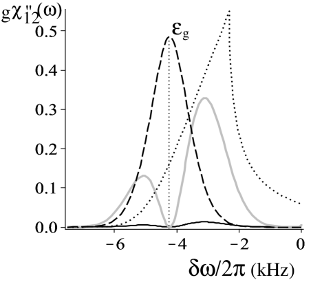
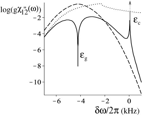
Figure 5: Imaginary susceptibility $\chi^{\prime\prime}_{12}$ of a bulk Bose condensed gas $\epsilon_{\mathbf{q}}=2\pi\times 30{\rm Hz}$ versus the detuning frequency $\delta\omega$. Parameter values are the ones of Fig.4. Left and right graphs represent the same curves but the right graph is in logarithm scale. The black dashed/solid curve is calculated in absence/presence of the screening factor while the dotted curve represents the Bogoliubov approximation. See the grey curve for a magnification of the black solid curve ($\times 25$)

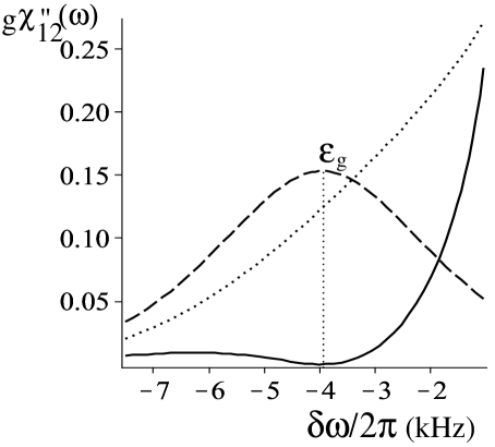
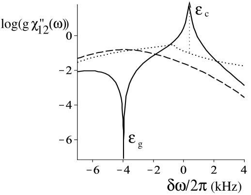
Figure 6: Idem as Fig.5 but for $\epsilon_{\mathbf{q}}=2\pi\times 300{\rm Hz}$. Here, the broadening of the curves is much more important.

The screening effect strongly reduces the Raman scattering and, in particular, forbids it for atoms with momentum $\mathbf{k}$ such that $\mathbf{k}.\mathbf{q}=0$. This case corresponds to $\delta\omega=\epsilon_{g}$ and includes also the condensed atoms ($\mathbf{k}=0$). The graphs illustrate well the effect of the macroscopic wave function that deforms its shape in order to attenuate locally the external potential displayed by the Raman light beams and to prevent incoherent scattering of the condensed atom. The experimental observation of this result would explain some of the reasons for which a superfluid condensate moves coherently without any friction with its surrounding. Anti-screening occurs in the region close to the resonance frequency $\epsilon_{c}$ of the collective mode. At zero temperature, we recover $\epsilon_{c}=\epsilon_{\mathbf{q}}$ Fetter while for non zero temperature the collective modes become damped for $\mathbf{q}\not=0$ gap .

These results can be compared to the one obtained from the Bogoliubov non conserving approximation developed in gap and valid only for a weakly depleted condensate. This approach implicitly assumes that the only elementary excitations are the collective ones and form a basis of quantum orthogonal states that describe the thermal part of the gas. Consequently, this formalism predicts no gap and no screening. Instead, the intercomponent susceptibility describes transitions involving the two collective excitation modes of phonon $\epsilon_{\mathbf{k}}^{B}$ and of rotation in spinor space $\epsilon_{\mathbf{k}}$:

$$\chi^{B}_{12}(\mathbf{q},\omega)=\frac{n_{\mathbf{0}}}{\omega-\epsilon_{\mathbf{q}}+i0}+\frac{1}{V}\sum_{\pm,\mathbf{k}}\frac{u^{2}_{\pm,\mathbf{k}}(n^{B}_{\mathbf{k}}+\delta_{\pm,-})}{\omega+i0\pm\epsilon^{B}_{\mathbf{k}}-\epsilon_{\mathbf{k}\pm\mathbf{q}}}$$ (66)

where $u_{\pm,\mathbf{k}}=\pm[(\epsilon_{\mathbf{k}}+gn_{\mathbf{0}})/2\epsilon^{B}_{\mathbf{k}}\pm 1/2]^{1/2}$. This function does not preserve the f-sum rule associated to the $SU(2)$ symmetry. In contrast to the GRPA, a delta peak describes a spinor rotation transition of the condensed fraction, and two other transitions involve the excitation transfer from a phonon mode into a rotation mode and the excitation creation in the two modes simultaneously. For small $\mathbf{q}$, these processes remain dispersive since the frequency transition depends on the momentum $\mathbf{k}$. As a consequence, the resulting spectrum shown in Figs. 5 and 6 is broader. In particular, the process of creation in the two modes favors transition with positive frequency. Note also the maximum of the curve separating the region involving a transition atom-atom like (high $\mathbf{k}$) and the one involving a transition phonon-atom like (low $\mathbf{k}$).

All these features established so far for the bulk case allow a clear comparison between the GRPA and the Bogoliubov approaches. In the real case of a parabolic trap, the inhomogeneity induces a supplementary broadening of the spectrum that prevents the direct observation of the screening. This effect as well as the finite time resolution and the difference between the scattering lengths will be discussed in a subsequent work.

V Conclusions and perspectives

We have analyzed the many body properties that can be extracted from the Raman scattering in the framework the GRPA. The calculated spectrum allows to show the existence of a second branch of excitation but also the screening effect which prevents the excitation of the condensed mode alone.

The observation of phenomena like the gap and the dynamical screening could have significant repercussions on our microscopic understanding of a finite temperature Bose condensed gas and its superfluidity mechanism. On the contrary, the non-observation of these phenomena would imply that the gapless and conserving GRPA is not valid. In that case, a different approximation has to be developed in order to explain what will be observed. As an alternative, the idea to use the Bogoliubov approach has been also discussed. But unfortunately, the violation of the f-sum rule is a serious concern regarding this non conserving approach gap . All these aspects emphasize the importance of the experimental study of the Raman scattering at finite temperature.

PN thanks the referees for usefull comments and acknowledges support from the Belgian FWO project G.0115.06, from the Junior fellowship F/05/011 of the KUL research council, and from the German AvH foundation.

References

• (1) P. SzΓ©pfalusy and I. Kondor, Ann. Phys. 82, 1-53 (1974); A. Minguzzi, M.P. Tozi, J. Phys.: Cond. Matter 9 10211 (1997); M. Fliesser, J. Reidl, P. SzΓ©pfalusy, R. Graham, Phys. Rev. A 64, 013609 (2001); J. Reidl, A. Csordas, R. Graham, P. SzΓ©pfalusy, Phys. Rev. A 61, 043606 (2000).
• (2) C.-H. Zhang and H.A. Fertig, Phys. Rev. A 74, 023613 (2006). C.-H. Zhang and H.A. Fertig, Phys. Rev. A 75, 013601 (2007).
• (3) P. Navez, J. Low. Temp. Phys. 138, 705-710 (2005); P. Navez, Physica A 356, 241-278 (2005); P. Navez and R. Graham, Phys. Rev. A 73, 043612 (2006).
• (4) M.Γ–. Oktel and L.S. Levitov, Phys. Rev. Lett. 83, 1 (1999); M.Γ–. Oktel and L.S. Levitov, Phys. Rev. A 65, 063604 (2002); M.Γ–. Oktel, T.C. Killian, D. Kleppner and L.S. Levitov, Phys. Rev. A 65, 033617 (2002); M.Γ–. Oktel and L.S. Levitov, Phys. Rev. Lett. 88, 230403 (2002).
• (5) P.Β Navez, Physica A 387, 4070 (2008).
• (6) A. Griffin, Phys. Rev. B 53, 9341 (1996); P.C. Hohenberg and P.C. Martin, Ann. Phys. (N.Y.) 34, 291 (1965); A. Griffin, Excitations in a Bose-Condensed Liquid (University Press, Cambridge, 1993).
• (7) N.M. Hugenholtz and D. Pines, Phys. Rev. 116, 489 (1959).
• (8) D.M. Stamper-Kurn, A.P. Chikkatur, A. GΓΆrlitz, S. Inouye, S. Gupta, D.E. Pritchard, and W. Ketterle, Phys. Rev. Lett. 83, 2876 (1999).
• (9) F. Zambelli, L. Pitaevskii, D.M. Stamper-Kurn and S. Stringari, Phys. Rev. A 61, 063608 (2000); R. Ozeri, N. Katz, J. Steinhauer, and N. Davidson, Rev. Mod. Phys. 77, 187 (2005).
• (10) A. J. Leggett, Rev. Mod. Phys. 73, 307 (2001); L. Pitaevskii and S. Stringari, Bose-Einstein Condensation, (Clarendon Press, 2003); C. J. Pethick and H. Smith, Bose-Einstein Condensation in Dilute Gases, (Cambridge University Press, 2001).
• (11) A. J. Leggett, Superfluidity, Rev. Mod. Phys. 71, S318 (1999).
• (12) A. P. Chikkatur, A. GΓΆrlitz, D. M. Stamper-Kurn, S. Inouye, S. Gupta, and W. Ketterle, Phys. Rev. Lett. 85, 483 (2000).
• (13) F. S. Cataliotti, S. Burger, C. Fort, P. Maddaloni, F. Minardi, A. Trombettoni, A. Smerzi, and M. Inguscio, Science 293, 843 (2001).
• (14) D. A. Huse and E.D. Siggia, J. Low. Temp. Phys. 46, 137 (1981).
• (15) D. Pines and P. NoziΓ¨res, The Theory of Quantum Liquids (Addison-Wesley, Readin, MA, 1989), Vol. I and II.
• (16) A. Montina, Phys. Rev. A 67, 053614 (2003); A. Montina, Phys. Rev. A 66, 023609 (2002)
• (17) W. B. Colson and A. L. Fetter, J. Low Temp. Phys. 33, 231 (1978); W. Zhang, D. L. Zhou, M.-S. Chang, M. S. Chapman, and L. You, Phys. Rev. Lett. 95, 180403 (2005).