Localisable moving average symmetric
stable and multistable processes

Abstract

We study a particular class of moving average processes which possess a property called localisability. This means that, at any given point, they admit a “tangent process”, in a suitable sense. We give general conditions on the kernel $g$ defining the moving average which ensures that the process is localisable and we characterize the nature of the associated tangent processes. Examples include the reverse Ornstein-Uhlenbeck process and the multistable reverse Ornstein-Uhlenbeck process. In the latter case, the tangent process is, at each time $t$, a Lévy stable motion with stability index possibly varying with $t$. We also consider the problem of path synthesis, for which we give both theoretical results and numerical simulations.

1 Introduction and background

In this work, we study moving average processes which are localisable. Loosely speaking, this means that they have a well-defined local form: at each point, they are “tangent” to a given stochastic process.

Localisable processes are useful both in theory and in practical applications. Indeed, they provide an easy way to control important local properties such as the local Hölder regularity or the jump intensity. In the first case, one speaks of multifractional processes, and in the second one, of multistable processes. Such processes provide fine models for real world phenomena including natural terrains, TCP traffic, financial data, EEG or highly textured images.

Formally, a process $Y(t)$ defined on $\mathbb{R}$ (or a subinterval of $\mathbb{R}$) is $h$-localisable at $u$ if $\lim_{r\to 0^{+}}r^{-h}(Y(u+rt)-Y(u))$ exists as a non-trivial process in $t$ for some $h>0$, where the convergence is in finite dimensional distributions, see [3, 4]. When convergence occurs in distribution with respect to the appropriate metric on $C(\mathbb{R})$ (the space of continuous functions on $\mathbb{R}$) or on $D(\mathbb{R})$ (the space of càdlàg functions on $\mathbb{R}$, that is functions which are continuous on the right and have left limits at all $t\in\mathbb{R}$), we say that $Y$ is strongly localisable. The limit, denoted by $Y_{u}^{\prime}=\{Y_{u}^{\prime}(t):t\in\mathbb{R}\}$, is called the local form or tangent process of $Y$ at $u$ and will in general vary with $u$. A closely related notion is that of locally asymptotically self-similar processes, which are for instance described in [2].

The simplest localisable processes are self-similar processes with stationary increments (sssi processes); it is not hard to show that an sssi process $Y$ is localisable at all $u$ with local form $Y_{u}^{\prime}=Y$. Furthermore, an sssi process $Y$ is strongly localisable if it has a version in $C(\mathbb{R})$ or $D(\mathbb{R})$.

In [5], processes with prescribed local form are constructed by “gluing together” known localisable processes in the following way: let $U$ be an interval with $u$ an interior point. Let $\{X(t,v):(t,v)\in U\times U\}$ be a random field and let $Y$ be the diagonal process $Y=\{X(t,t):t\in U\}$. In order for $Y$ and $X(\cdot,u)$ to have the same local forms at $u$, that is $Y_{u}^{\prime}(\cdot)=X_{u}^{\prime}(\cdot,u)$ where $X_{u}^{\prime}(\cdot,u)$ is the local form of $X(\cdot,u)$ at $u$, we require

$$\frac{X(u+rt,u+rt)-X(u,u)}{r^{h}}\stackrel{{\scriptstyle{\rm fdd}}}{{\rightarrow}}X_{u}^{\prime}(t,u)$$ (1.1)

as $r\searrow 0$.

This approach allows easy construction of localisable processes from “elementary pieces” which are known to be themselves localisable. In particular, it applies in a straightforward way to processes $X(t,v)$ such that $X(\cdot,v)$ is sssi for each $v$.

In this work we shall study a rather different way of obtaining localisable processes. Instead of basing our constructions on existing sssi processes we will consider moving average processes which, as we shall see, provide a new class of localisable $\alpha$-stable processes.

The remainder of this paper is organized as follows: in section 2, we give general conditions on the kernel $g$ defining the moving average process to ensure (strong) localisability. Section 3 specializes these conditions to cases where explicit forms for the tangent process may be given, and presents some examples. In section 4, we deal with multistable moving average processes, which generalize moving average stable processes by letting the stability index vary over time. Finally, section 5 considers numerical aspects: for applications, it is desirable to synthesize paths of these processes. Using the approach developed in [12], we first explain how to build traces of arbitrary moving average stable processes. In the case where the processes are localisable, we then give error bounds between the numerical and theoretical paths. Under mild additional assumptions, an ‘optimal’ choice of the parameters defining the synthesis method is derived. Finally, traces obtained from numerical experiments are displayed.

2 Localisability of stable moving average processes

Recall that a process $\{X(t):t\in T\}$, where $T$ is a subinterval of $\mathbb{R}$, is called $\alpha$-stable $(0<\alpha\leq 2)$ if all its finite-dimensional distributions are $\alpha$-stable, see the encyclopaedic work on stable processes [10]. $2$-stable processes are just Gaussian processes.

Many stable processes admit a stochastic integral representation. Write $S_{\alpha}(\sigma,\beta,\mu)$ for the $\alpha$-stable distribution with scale parameter $\sigma$, skewness $\beta$ and shift-parameter $\mu$; we will assume throughout that $\beta=\mu=0$. Let $(E,{\cal E},m)$ be a sigma-finite measure space ($m$ will be Lebesgue measure in our examples). Taking $m$ as the control measure, this defines an $\alpha$-stable random measure $M$ on $E$ such that for $A\in{\cal E}$ we have that $M(A)\sim S_{\alpha}(m(A)^{1/\alpha},0,0)$ (since $\beta=0$, the process is symmetric).

Let

$${\cal F}_{\alpha}\equiv{\cal F}_{\alpha}(E,{\cal E},m)=\{f:f\mbox{ is measurable and }\|f\|_{\alpha}<\infty\},$$

where $\|\,\|_{\alpha}$ is the quasinorm (or norm if $1<\alpha\leq 2$) given by

$$\|f\|_{\alpha}=\left(\int_{E}|f(x)|^{\alpha}m(dx)\right)^{1/\alpha}.$$ (2.1)

The stochastic integral of $f\in{\cal F}_{\alpha}(E,{\cal E},m)$ with respect to $M$ then exists [10, Chapter 3] with

$$\int_{E}f(x)M(dx)\sim S_{\alpha}(\sigma_{f},0,0),$$ (2.2)

where $\sigma_{f}=\|f\|_{\alpha}$.

We will be concerned with a special kind of stable processes that are stationary and may be expressed as moving average stochastic integrals in the following way:

$$Y(t)=\int g(t-x)M(dx)\quad(t\in\mathbb{R}),$$ (2.3)

where $g\in{\cal F}_{\alpha}$ is sometimes called the kernel of $Y$.

Such processes are considered in several areas (e.g. linear time-invariant systems) and it is of interest to know under what conditions they are localisable. A sufficient condition is provided by the following proposition.

Proposition 2.1

Let $0<\alpha\leq 2$ and let $M$ be a symmetric $\alpha$-stable measure on $\mathbb{R}$ with control measure Lebesgue measure ${\cal L}$. Let $g\in{\cal F}_{\alpha}$ and let $Y$ be the moving average process

$$Y(t)=\int g(t-x)M(dx)\quad(t\in\mathbb{R}).$$

Suppose that there exist jointly measurable functions $h(t,.)\in{\cal F}_{\alpha}$ such that

$$\lim_{r\to 0^{+}}\int\left|\frac{g(r(t+z))-g(rz)}{r^{\gamma}}-h(t,z)\right|^{\alpha}dz=0$$ (2.4)

for all $t\in\mathbb{R}$, where $\gamma+1/\alpha>0$. Then $Y$ is $(\gamma+1/\alpha)$-localisable with local form $Y^{\prime}_{u}=\{\int h(t,z)M(dz):t\in\mathbb{R}\}$ at all $u\in\mathbb{R}$.

Proof. Using stationarity followed by a change of variable $z=-x/r$ and the self-similarity of $M$,

$$Y(u+rt)-Y(u) = Y(rt)-Y(0)$$

$$= \int(g(rt-x)-g(-x))M(dx)$$

$$= r^{1/\alpha}\int(g(r(t+z))-g(rz))M(dz),$$

where equalities are in finite dimensional distributions. Thus

$$\frac{Y(u+rt)-Y(u)}{r^{\gamma+1/\alpha}}-\int h(t,z)M(dz)=\int\left(\frac{g(r(t+z))-g(rz)}{r^{\gamma}}-h(t,z)\right)M(dz).$$

By [10, proposition 3.5.1] and (2.4), $r^{-\gamma-1/\alpha}(Y(u+rt)-Y(u))\to\int h(t,z)M(dz)$ in probability and thus in finite dimensional distributions.  

A particular instance of (2.3) is the reverse Ornstein-Uhlenbeck process, see [10, Section 3.6]. This process provides a straightforward application of proposition 2.1.

Proposition 2.2

(Reverse Ornstein-Uhlenbeck process) Let $\lambda>0$ and $1<\alpha\leq 2$ and let $M$ be an $\alpha$-stable measure on $\mathbb{R}$ with control measure ${\cal L}$. The stationary process

$$Y(t)=\int_{t}^{\infty}\exp(-\lambda(x-t))M(dx)\quad(t\in\mathbb{R})$$

has a version in $D(\mathbb{R})$ that is $1/\alpha$-localisable at all $u\in\mathbb{R}$ with $Y_{u}^{\prime}=L_{\alpha}$, where $L_{\alpha}(t):=\int_{0}^{t}M(dz)$ is $\alpha$-stable Lévy motion.

Proof. The process $Y$ is a moving average process that may be written in the form (2.3) with $g(x)=\exp(\lambda x){\bf 1}_{(-\infty,0]}(x)$. It is easily verified using the dominated convergence theorem that $g$ satisfies (2.4) with $\gamma=0$ and $h(t,z)=-{\bf 1}_{(-t,0]}(z)$ for $t\geq 0$ and $h(t,z)=-{\bf 1}_{(0,-t]}(z)$ for $t<0$, so proposition 2.1 gives the conclusion with $Y_{u}^{\prime}(t)=-M([-t,0])=L_{\alpha}(t)$ for $t\geq 0$ and a similar formula for $t<0$.  

Proposition 2.1 gives a condition on the kernel ensuring localisability. With an additional constraint we can get strong localisability. First we need the following proposition on continuity.

Proposition 2.3

Let $0<\alpha<2$, $g\in\mathcal{F}_{\alpha}$ and let $M$ be an $\alpha$-stable symmetric random measure on $\mathbb{R}$ with control measure $\mathcal{L}$. Consider the moving average process defined by (2.3). Suppose that $g$ satisfies, for all sufficiently small $h$,

$$\int\left|g(h-x)-g(-x)\right|^{\alpha}dx\leq c|h|^{\lambda},$$

where $c>0$ and $\lambda>1$. Then $Y$ has a continuous version which satisfies a $\theta$-Hölder condition for all $\theta<(\lambda-1)/\alpha$.

Proof. By stationarity,

$$Y(t)-Y(t^{\prime}) = Y(t-t^{\prime})-Y(0)$$

$$= \int\left(g(t-t^{\prime}-x)-g(-x)\right)M(dx).$$

So for $0<p<\alpha$

$$\mbox{\sf E}|Y(t)-Y(t^{\prime})|^{p} \leq c_{1}\left(\int\left|g(t-t^{\prime}-x)-g(-x)\right|^{\alpha}dx\right)^{p/\alpha}$$

$$\leq c_{2}|t-t^{\prime}|^{\lambda p/\alpha}.$$

The result then follows from the Kolmogorov criterion by taking $p$ arbitrarily close to $\alpha$.  

Proposition 2.4

With the same notation and assumptions as in proposition 2.1, suppose that in addition that $g$ satisfies, for all sufficiently small $h$,

$$\int\left|g(h-x)-g(-x)\right|^{\alpha}dx\leq c|h|^{\alpha\gamma+1},$$ (2.5)

where $c>0$ and $\gamma>0$. Then $Y$ has a version in $C(\mathbb{R})$ that is $(\gamma+1/\alpha)$-strongly localisable with $Y^{\prime}_{u}=\{\int h(t,z)M(dz):t\in\mathbb{R}\}$ at all $u\in\mathbb{R}$.

Proof. By proposition 2.3, $Y(t)$ has a continuous version and so $Z_{r}(t):=r^{-(\gamma+1/\alpha)}(Y(rt)-Y(0))$ also has a continuous version. Thus, for $0<p<\alpha$, by stationarity and setting $h=r|t-t^{\prime}|$ sufficiently small,

$$\mbox{\sf E}|Z_{r}(t)-Z_{r}(t^{\prime})|^{p} = \mbox{\sf E}|Z_{r}(t-t^{\prime})-Z_{r}(0)|^{p}$$

$$= c_{1}\left(\int\left|\frac{g(r(t-t^{\prime})-x)-g(-x)}{r^{\gamma+1/\alpha}}\right|^{\alpha}dx\right)^{p/\alpha}$$

$$= c_{1}\left(\int\frac{|g(h-x)-g(-x)|^{\alpha}}{h^{\gamma\alpha+1}}dx\right)^{p/\alpha}|t-t^{\prime}|^{(\gamma\alpha+1)p/\alpha}$$

$$\leq c_{2}|t-t^{\prime}|^{(\gamma\alpha+1)p/\alpha},$$

provided $|t-t^{\prime}|$ is sufficiently small, using (2.5) in the last step. We may choose $p$ sufficiently close to $\alpha$ so that $(\gamma\alpha+1)p/\alpha>1$. By a Corollary to Kolmogorov’s criterion (see e.g. [9, Theorem 85.5]) the measures on $C(\mathbb{R})$ underlying the processes $Z_{r}$ are conditionally compact. Thus convergence in finite dimensional distributions of $Z_{r}$ to $Y^{\prime}_{u}$ as $r\searrow 0$ implies the convergence in distribution (with $Y^{\prime}_{u}$ necessarily having a continuous version). Together with localisability which follows from proposition 2.1 this gives strong localisability.  

Note that the reverse Ornstein-Uhlenbeck process is a stationary Markov process which has a version in $D(\mathbb{R})$ see [11, Remark 17.3]. It also satisfies (2.5) for $\alpha\geq 1$ with $\gamma=0$. However, we cannot deduce that it is strongly localisable since proposition 2.4 is only valid for $\gamma>0$. The case $\gamma=0$ would be interesting to deal with, but is much harder and would require different techniques.

3 Sufficient conditions for localisability and examples

For the reverse Ornstein-Uhlenbeck process, it was straightforward to check the conditions of proposition 2.1. In general, however, it is not easy to guess which kind of functions $g$ in $\mathcal{F}_{\alpha}$ will satisfy (2.4). In this section we will find simple practical conditions ensuring this.

Recall that the following process is called linear fractional $\alpha$-stable motion:

$$L_{\alpha,H,b^{+},b^{-}}(t)=\int_{-\infty}^{\infty}f_{\alpha,H}(b^{+},b^{-},t,x)M(dx),$$

where $t\in\mathbb{R}$, $b^{+},b^{-}\in\mathbb{R}$, and

$$f_{\alpha,H}(b^{+},b^{-},t,x)=b^{+} \left((t-x)_{+}^{H-1/\alpha}-(-x)_{+}^{H-1/\alpha}\right)$$

$$+b^{-}\left((t-x)_{-}^{H-1/\alpha}-(-x)_{-}^{H-1/\alpha}\right),$$ (3.1)

where $M$ is a symmetric $\alpha$-stable random measure $(0<\alpha<2)$ with control measure Lebesgue measure. Being sssi, $L_{\alpha,H,b^{+},b^{-}}$ is localisable. In addition, it is strongly localisable when $H>1/\alpha$, since its paths then belong to $C(\mathbb{R})$.

Recall also that the process

$$L_{\alpha}(t)=\int_{0}^{t}M(dx)$$ (3.2)

is $\alpha$-stable Lévy motion and the process

$$Z_{\alpha}(t)=\int_{-\infty}^{+\infty}(\ln|t-x|-\ln|x|)M(dx)$$ (3.3)

is called log-fractional stable motion.

We are now ready to describe easy-to-check conditions that ensure that propositions 2.1 and 2.4 apply.

Proposition 3.1

Let $0<\alpha\leq 2$, $g\in\mathcal{F}_{\alpha}$ and $M$ be an $\alpha$-stable symmetric random measure on $\mathbb{R}$ with control measure $\mathcal{L}$. Let $Y$ be the moving average process

$$Y(t)=\int g(t-x)M(dx)\hskip 14.22636pt(t\in\mathbb{R}).$$

If there exist $c_{0}^{+},c_{0}^{-},\gamma,a,c,\eta\in\mathbb{R}$ with $c>0$, $\eta>0$ and $0<\gamma+1/\alpha<a\leq 1$ such that

$$\frac{g(r)}{r^{\gamma}}\rightarrow c_{0}^{+}\textrm{ and }\frac{g(-r)}{r^{\gamma}}\rightarrow c_{0}^{-}$$

as $r\searrow 0$ and

$$\left|g(u+h)-g(u)\right|\leq c|h|^{a}|u|^{\gamma-a}\quad(u\in\mathbb{R},|h|<\eta),$$ (3.4)

then $Y$ is $(\gamma+1/\alpha)$-localisable at all $u\in\mathbb{R}$ with local form

$$\begin{array}[]{ll}(a)&Y^{\prime}_{u}=L_{\alpha,\gamma+1/\alpha,c_{0}^{+},c_{0}^{-}}\quad\textrm{if }\gamma\neq 0,\\ &\\ (b)&Y^{\prime}_{u}=(c_{0}^{+}-c_{0}^{-})L_{\alpha}\quad\textrm{if }\gamma=0.\\ \end{array}$$

If, in addition, $\gamma>0$ and $0<\alpha<2$ then $Y$ has a version in $C(\mathbb{R})$ and is strongly localisable.

Note that condition (3.4) on the increments of $g$ may be interpreted as a 2-microlocal condition, namely that $g$ belongs to the global 2-microlocal space $C_{0}^{\gamma,a-\gamma}$, see [7]. Remark also that, in order for this condition to be satisfied by non-trivial functions $g$, one needs $a\leq 1$, which in turns implies that $\gamma\leq 1-1/\alpha$ and $a-\gamma\in(1/\alpha,1-\gamma]$.

Proof (a) We have

$$\frac{g(r(t+z))-g(rz)}{r^{\gamma}}=\frac{g(r|t+z|)}{(r|t+z|)^{\gamma}} |t+z|^{\gamma}\mathbf{1}_{\{t+z\geq 0\}}+\frac{g(-r|t+z|)}{(r|t+z|)^{\gamma}}|t+z|^{\gamma}\mathbf{1}_{\{t+z<0\}}$$

$$-\frac{g(r|z|)}{(r|z|)^{\gamma}}|z|^{\gamma}\mathbf{1}_{\{z\geq 0\}}-\frac{g(-r|z|)}{(r|z|)^{\gamma}}|z|^{\gamma}\mathbf{1}_{\{z<0\}}.$$

As $r\to 0$,

$$\frac{g(r(t+z))-g(rz)}{r^{\gamma}} \rightarrow c_{0}^{+}|t+z|^{\gamma}\mathbf{1}_{\{t+z\geq 0\}}+c_{0}^{-}|t+z|^{\gamma}\mathbf{1}_{\{t+z<0\}}-c_{0}^{+}|z|^{\gamma}\mathbf{1}_{\{z\geq 0\}}-c_{0}^{-}|z|^{\gamma}\mathbf{1}_{\{z<0\}}$$

$$= c_{0}^{+}(t+z)_{+}^{\gamma}-c_{0}^{+}(z)_{+}^{\gamma}+c_{0}^{-}(t+z)_{-}^{\gamma}-c_{0}^{-}(z)_{-}^{\gamma}$$

$$= f_{\alpha,\gamma+1/\alpha}(c_{0}^{+},c_{0}^{-},t,-z).$$

To get convergence in $L^{\alpha}$ we use the dominated convergence theorem. Fix $\epsilon>0$ and $m>0$ such that for all $0<u<\epsilon$,

$$\left|\frac{g(u)}{u^{\gamma}}-c_{0}^{+}\right|\leq m\textrm{ and }\left|\frac{g(-u)}{u^{\gamma}}-c_{0}^{-}\right|\leq m.$$

For fixed $t$ write $f_{r}(z)=r^{-\gamma}(g(r(t+z))-g(rz))$. If $t=0$,

$$f_{r}(z)=f_{\alpha,\gamma+1/\alpha}(c_{0}^{+},c_{0}^{-},t,-z)=0,$$

thus $f_{r}\to f_{\alpha,\gamma+1/\alpha}(c_{0}^{+},c_{0}^{-},t,-.)$ which belongs to $L^{\alpha}$. Assume now $t\in\mathbb{R}^{*}$. There is a constant $m_{1}$ such that $|f_{r}(z)|^{\alpha}\leq m_{1}(1+|z|^{\gamma}+|t+z|^{\gamma})^{\alpha}$ for all $|r|\leq\frac{\epsilon}{1+|t|}$ and $|z|\leq 1$. From (3.4)

$$|f_{r}(z)|^{\alpha}\leq\left(\frac{|rt|^{a}|rz|^{\gamma-a}}{|r|^{\gamma}}\right)^{\alpha}\leq|t|^{a\alpha}|z|^{(\gamma-a)\alpha}$$

for $|r|<\eta/|t|$, so, as $(\gamma-a)\alpha<-1$ and $\gamma\alpha>-1$,

$$\int_{|z|\leq 1}m_{1}(1+|z|^{\gamma}+|t+z|^{\gamma})^{\alpha}dz+\int_{|z|>1}|z|^{(\gamma-a)\alpha}dz<\infty.$$

Since also $f_{\alpha,\gamma+1/\alpha}(c_{0}^{+},c_{0}^{-},t,-z)\in L^{\alpha}$, the dominated convergence theorem implies that $f_{r}(z)\to f_{\alpha,\gamma+1/\alpha}(c_{0}^{+},c_{0}^{-},t,-z)$ in $L^{\alpha}$. The conclusion in case (a) follows from proposition 2.1, (3.1), and noting that $M$ is a symmetric $\alpha$-stable measure.

(b) In this case the limit (3) is

$$\frac{g(r(t+z))-g(rz)}{r^{\gamma}}\to\left\{\begin{array}[]{rcl}(c_{0}^{+}-c_{0}^{-})\mathbf{1}_{[0,t]}(-z)&\mbox{ if }&t\geq 0\\ -(c_{0}^{+}-c_{0}^{-})\mathbf{1}_{[t,0]}(-z)&\mbox{ if }&t<0\\ \end{array}\right..$$

Dominated convergence follows in the same way as in case (a) so the conclusion follows from proposition 2.1 and (3.2).

Moving to strong localisability, for $h$ small enough,

$$\int_{|x|\leq 3|h|}|g(h-x)-g(-x)|^{\alpha}dx\leq c_{1}\int_{|x|\leq 3|h|}|h|^{\alpha\gamma}dx\leq c_{2}|h|^{\alpha\gamma+1},$$

and

$$\int_{|x|\geq 3|h|}|g(h-x)-g(-x)|^{\alpha}dx \leq c_{1}|h|^{a\alpha}\int_{3|h|}^{\infty}|x|^{(\gamma-a)\alpha}dx$$

$$\leq c_{2}|h|^{a\alpha}|h|^{1+(\gamma-a)\alpha}$$

$$= c_{2}|h|^{\alpha\gamma+1}$$

and the conclusion follows from propositions 2.3 and 2.4.  

We now give an alternative condition for localisability in terms of Fourier transforms. Note that the Fourier transform $\widehat{f}_{\alpha,H}(b^{+},b^{-},t,\xi)$ of $f_{\alpha,H}(b^{+},b^{-},t,.)$ is given by

$$\widehat{f}_{\alpha,H}(b^{+},b^{-},t,\xi)= \Gamma(H+1-1/\alpha)\frac{e^{-i\xi t}-1}{|\xi|^{H+1-1/\alpha}}$$

$$\times\left[b^{+}\exp\Big{(}\frac{i\pi}{2}\textrm{sgn}(\xi)(H+1-1/\alpha)\Big{)}+b^{-}\exp\Big{(}-\frac{i\pi}{2}\textrm{sgn}(\xi)(H+1-1/\alpha\Big{)}\right].$$

Proposition 3.2

Let $1\leq\alpha\leq 2$, and $Y$ be defined by (2.3). If there exist $l=l_{1}+il_{2}\in\mathbb{C}^{*}$, $\gamma\in(-\frac{1}{\alpha},1-\frac{1}{\alpha})$, $a\in(0,1-(\gamma+\frac{1}{\alpha}))$ and $K\in L^{p}(\mathbb{R})$ with $p\in[1,1/(\gamma+\frac{1}{\alpha}+a))$, such that for almost all $\xi>0$,

$$\xi^{\gamma+1}\widehat{g}(\xi)=l+\frac{1}{\xi^{a}}\widehat{K}(\xi),$$ (3.6)

then $Y$ is $(\gamma+1/\alpha)$-localisable at all $u\in\mathbb{R}$ with local form

$$\begin{array}[]{ll}(a)&Y^{\prime}_{u}=L_{\alpha,\gamma+1/\alpha,b^{+},b^{-}}\quad\textrm{if }\gamma\neq 0\\ &\\ (b)&Y^{\prime}_{u}=\frac{1}{\pi}l_{1}Z_{\alpha}+l_{2}L_{\alpha}\quad\textrm{if }\gamma=0,\\ \end{array}$$

where

$$b^{+}=\frac{1}{2\Gamma(\gamma+1)}\left(\frac{l_{1}}{\cos(\pi(\gamma+1)/2)}-\frac{l_{2}}{\sin(\pi(\gamma+1)/2)}\right),$$

$$b^{-}=\frac{1}{2\Gamma(\gamma+1)}\left(\frac{l_{1}}{\cos(\pi(\gamma+1)/2)}+\frac{l_{2}}{\sin(\pi(\gamma+1)/2)}\right).$$

Proof (a) First note that, with $b^{+}$ and $b^{-}$ as above, we have, for $z\neq 0$,

$$\widehat{f}_{\alpha,\gamma+1/\alpha}(b^{+},b^{-},t,\xi)=\frac{e^{-i\xi t}-1}{|\xi|^{\gamma+1}}(\bar{l}\mathbf{1}_{\xi>0}+l\mathbf{1}_{\xi<0}).$$

Set $f_{r}(z)=r^{-\gamma}(g(r(t+z))-g(rz))$. Then $f_{r}\in\mathcal{F}_{\alpha}$ and

$$\widehat{f}_{r}(\xi)=\frac{e^{i\xi t}-1}{r^{\gamma+1}}\widehat{g}\big{(}\frac{\xi}{r}\big{)}.$$

With $\alpha^{\prime}$ such that $\frac{1}{\alpha}+\frac{1}{\alpha^{\prime}}=1$ we have $\widehat{f}_{r}\in\mathcal{F}_{\alpha^{\prime}}$ and $\widehat{f}_{\alpha,\gamma+1/\alpha}(b^{+},b^{-},t,\xi)\in\mathcal{F}_{\alpha^{\prime}}$. We now show that $\|f_{r}-f_{\alpha,\gamma+1/\alpha}(b^{+},b^{-},t,-\cdot)\|_{\alpha}\rightarrow 0$ when $r\rightarrow 0$. Note that (3.6) implies that for $\xi<0$

$$|\xi|^{\gamma+1}\widehat{g}(\xi)=\bar{l}+\frac{1}{|\xi|^{a}}\widehat{K}(\xi).$$

Writing $\widehat{f}(\xi)=\widehat{f}_{\alpha,\gamma+1/\alpha}(b^{+},b^{-},t,-\xi)$, for almost all $\xi\in\mathbb{R}$

$$\widehat{f}_{r}(\xi)-\widehat{f}(\xi) = \frac{(e^{i\xi t}-1)}{|\xi|^{\gamma+1}}\left(\Big{(}\frac{|\xi|^{\gamma+1}}{r^{\gamma+1}}\widehat{g}\big{(}\frac{\xi}{r}\big{)}-l\Big{)}\mathbf{1}_{\xi>0}+\Big{(}\frac{|\xi|^{\gamma+1}}{r^{\gamma+1}}\widehat{g}\big{(}\frac{\xi}{r}\big{)}-\bar{l}\Big{)}\mathbf{1}_{\xi<0}\right)$$

$$= \frac{(e^{i\xi t}-1)}{|\xi|^{\gamma+1}}\frac{r^{a}}{|\xi|^{a}}K\big{(}\frac{\xi}{r}\big{)}$$

$$= r^{a}\frac{(e^{i\xi t}-1)}{|\xi|^{\gamma+1+a}}K\big{(}\frac{\xi}{r}\big{)}.$$

Let $H_{r}(u)=K(ru)$. Then $\widehat{H}_{r}(\xi)=\frac{1}{r}\widehat{K}(\frac{\xi}{r})$ and we may write for $a+\gamma\neq 0$

$$\widehat{f}_{r}(\xi)-\widehat{f}(\xi) = r^{a+1}\widehat{f}_{\alpha,\gamma+1/\alpha+a}(b,b,t,-\xi)\widehat{H_{r}}(\xi),$$ (3.7)

where $b=1/(2\Gamma(\gamma+a+1)\cos(\pi(\gamma+a+1)/2))$.

It is easy to verify that $f_{\alpha,\gamma+a+1/\alpha}(b^{+},b^{-},t,-\cdot)\in L_{\beta}$ for all $\beta>1/(1-\gamma-a)$. By the conditions on $\alpha$ and $p$, there exists such a $\beta$ which also satisfies $\frac{1}{\alpha}+1=\frac{1}{\beta}+\frac{1}{p}$ and in particular, $\frac{1}{p}+\frac{1}{\beta}>1$. Consequently we may take the inverse Fourier transform of (3.7) see, for example, [13, Theorem 78] to get:

$$f_{r}(z)-f(z)=r^{a+1}f_{\alpha,\gamma+1/\alpha+a}(b^{+},b^{-},t,-.)*H_{r}(z)$$

where $*$ denotes convolution. As $\frac{1}{\alpha}+1=\frac{1}{\beta}+\frac{1}{p}$, the Hausdorff-Young inequality yields

$$\|f_{r}-f_{\alpha,\gamma+1/\alpha}(b^{+},b^{-},t,-\cdot)\|_{\alpha} \leq r^{a+1}\|f_{\alpha,\gamma+1/\alpha+a}\|_{\beta}\|H_{r}\|_{p}$$

$$\leq r^{a+1-\frac{1}{p}}\|f_{\alpha,\gamma+1/\alpha+a}\|_{\beta}\|K\|_{p}.$$

We conclude that $f_{r}\rightarrow f_{\alpha,\gamma+1/\alpha}(b^{+},b^{-},t,-\cdot)$ in $L^{\alpha}$. The result follows from proposition 2.1. The case $a+\gamma=0$ is dealt with in a similar way.

(b) Let $z_{t}$ and $l_{t}$ be defined by

$$l_{t}(x)=\left\{\begin{array}[]{rl}\mathbf{1}_{]0,t[}(x)&\mbox{ if }t\geq 0\\ -\mathbf{1}_{]t,0[}(x)&\mbox{ if }t<0\\ \end{array}\right.$$

and

$$z_{t}(x)=\ln|t-x|-\ln|x|.$$

A straightforward computation shows that

$$z_{t}(x)=\mbox{sgn}(-t)\lim_{\varepsilon\rightarrow 0}\int_{|s|\geq\varepsilon}\frac{1}{s}\mathbf{1}_{[\min(x-t,x),\max(x-t,x)]}(s)ds,$$

so that, in the space of distributions we get

$$z_{t}=-\mbox{PV}(1/\cdot)*l_{t}$$

where PV denotes the Cauchy principal value. Thus

$$\widehat{z_{t}}(\xi) = -\widehat{\mbox{PV}(1/\cdot)}(\xi)\widehat{l_{t}}(\xi)$$

$$= -(-i\pi\mbox{sgn}(\xi))\big{(}-\frac{1}{i\xi}(e^{-i\xi t}-1)\big{)}$$

$$= -\pi\frac{e^{-i\xi t}-1}{|\xi|}.$$

With $f(z)=-\frac{1}{\pi}l_{1}z_{t}(-z)-l_{2}l_{t}(-z)$, we obtain

$$\widehat{f}(\xi)=\frac{e^{i\xi t}-1}{|\xi|}(l\mathbf{1}_{\xi>0}+\bar{l}\mathbf{1}_{\xi<0}).$$

As in (a) we conclude that $f_{r}\rightarrow f$ in $L^{\alpha}$. proposition 2.1 implies that $Y$ is $(\gamma+1/\alpha)$-localisable at all $u\in\mathbb{R}$ with local form $Y^{\prime}_{u}=\frac{1}{\pi}l_{1}Z_{\alpha}+l_{2}L_{\alpha}$, since $M$ is symmetric.  

We give examples to illustrate propositions 3.1 and 3.2.

Example 3.3

Let $\frac{6}{5}<\alpha\leq 2$ and let $M$ be an $\alpha$-stable symmetric random measure on $\mathbb{R}$ with control measure $\mathcal{L}$. Let

$$g(x)=\left\{\begin{array}[]{c c}0&(x\leq 0)\\ x^{1/6}&(0<x\leq 1)\\ x^{-5/6}&(x\geq 1)\\ \end{array}\right..$$

The stationary process defined by

$$Y(t)=\int g(t-x)M(dx)\hskip 11.38092pt(t\in\mathbb{R})$$

is $(1/6+1/\alpha)$-strongly localisable at all $u\in\mathbb{R}$ with local form $Y^{\prime}_{u}=L_{\alpha,1/6+1/\alpha,1,0}$.

Proof. We apply proposition 3.1 case (a) with $\alpha\in(\frac{5}{6},2]$. The function $g$ satisfies the assumptions with $\gamma=\frac{1}{6}$, $c_{0}^{+}=1$, $c_{0}^{-}=0$ and $a=1$.  

To verify condition (3.6) of proposition 3.2, one needs to check that $g\in L^{\alpha}(\mathbb{R})$ and also that $\xi^{a+\gamma+1}\widehat{g}(\xi)-l\xi^{a}$ is the Fourier transform of a function in $L^{p}(\mathbb{R})$ for some $a,\gamma,p$ in the admissible ranges. For this purpose, one may for instance apply classical theorems such as in [13, Theorems 82-84]. We give below an example that uses a direct approach.

Example 3.4

For $1\leq\alpha<2$ let $M$ be an $\alpha$-stable symmetric random measure on $\mathbb{R}$ with control measure $\mathcal{L}$. Let $g$ be defined by its Fourier transform

$$\widehat{g}(\xi)=\left\{\begin{array}[]{c c}0&(|\xi|\leq 1)\\ |\xi|^{-\gamma-1}&(|\xi|>1)\end{array}\right.$$

where $\gamma\in(-\frac{1}{\alpha},\frac{1}{2}-\frac{1}{\alpha})\subseteq(-1,0)$. Then $g\in L^{\alpha}(\mathbb{R})$ and the moving average process

$$Y(t)=\int g(t-x)M(dx)\hskip 11.38092pt(t\in\mathbb{R})$$

is well-defined and $\alpha$-localisable at all $u\in\mathbb{R}$, with local form $Y^{\prime}_{u}=L_{\alpha,\gamma+1/\alpha,b,b}$, where $b=-1/(2\Gamma(\gamma+1)\cos(\pi(\gamma+1/2)))$.

Proof. Taking $\widehat{K}(\xi)=|\xi|^{1/2}\mathbf{1}_{[-1,1]}(\xi)$ with $l=-1$ and $a=\frac{1}{2}$ in (3.6) gives $g$. To check that $K\in L^{p}(\mathbb{R})$ for all $p>1$, note that $K$ is continuous (in fact $C^{\infty}$) and that $|K(x)|\leq C|x|^{-1}$ for all $x$. Then $Y(t)$ will be well-defined if $g$ is in $L^{\alpha}(\mathbb{R})$. To verify this, one computes the inverse Fourier transform of $\widehat{g}$, to get $g(x)=2(\gamma+1)|x|^{\gamma}\int_{|x|}^{\infty}|v|^{-\gamma-2}\sin vdv-2x^{-1}\sin x$. By proposition 3.2(a), $Y$ is $\alpha$-localisable at all $u\in\mathbb{R}$ with the local form as stated.  

The approach of this example may be be used for general classes of functions $g$.

4 Multistable moving average processes

In [5], localisability is used to define multistable processes, that is processes which at each point $t\in\mathbb{R}$ have an $\alpha(t)$-stable random process as their local form, where $\alpha(t)$ is a sufficiently smooth function ranging in $(0,2)$. Thus such processes “look locally like” a stable process at each $t$ but with differing stability indices as time evolves.

Before we recall how this was done in [5], we note briefly that “stable-like” processes have been defined and studied in [8]. These stable-like processes are Markov jump processes, and are, in a sense, “localisable”, but with localisability defined by the requirement that they are solutions of an order $\alpha(x)$ fractional stochastic differential equations. See Theorem 2.1 in [8], which shows that the local form of sample paths is considered rather than of the limiting process. Another essential difference is that stable-like processes are Markov, whereas, in general, multistable ones, as defined below, are not. In fact, formula (4.6), where a Poisson process element Y is independent of t but is raised to a power that involves t means that our processes are “far” from Markov.

We now come back to our multistable processes. One route to defining such processes is to rewrite stable integrals as countable sums over Poisson processes. We recall briefly how this can be done, see [5] for fuller details. Let $(E,{\cal E},m)$ be a $\sigma$-finite measure space and let $\Pi$ be a Poisson process on $E\times\mathbb{R}$ with mean measure $m\times{\cal L}$. Thus $\Pi$ is a random countable subset of $E\times\mathbb{R}$ such that, writing $N(A)$ for the number of points in a measurable $A\subset E\times\mathbb{R}$, the random variable $N(A)$ has a Poisson distribution of mean $(m\times{\cal L})(A)$ with $N(A_{1}),\ldots,N(A_{n})$ independent for disjoint $A_{1},\ldots,A_{n}\subset E\times\mathbb{R}$, see [6]. In the case of constant $\alpha$, with $M$ a symmetric $\alpha$-stable random measure on $E$ with control measure $m$, one has, for $f\in{\cal F}_{\alpha}$ ([10, Section 3.12]),

$$\int f(x)M(dx)\,=\,c(\alpha)\sum_{({\sf X},{\sf Y})\in\Pi}f({\sf X}){\sf Y}^{<-1/\alpha>}\quad(0<\alpha<2),$$ (4.1)

where

$$c(\alpha)=\left(2\alpha^{-1}\Gamma(1-\alpha)\cos(\textstyle{\frac{1}{2}}\pi\alpha)\right)^{-1/\alpha},$$ (4.2)

and $a^{<b>}=\mbox{sign}(a)|a|^{b}$.

Now define the random field

$$X(t,v)=\sum_{({\sf X},{\sf Y})\in\Pi}f(t,v,{\sf X}){\sf Y}^{<-1/\alpha(v)>}.$$ (4.3)

Under certain conditions the “diagonal” process $X(t,t)$ gives rise to a multistable process with varying $\alpha$ of the form

$$Y(t)\equiv X(t,t)=\sum_{({\sf X},{\sf Y})\in\Pi}f(t,t,{\sf X}){\sf Y}^{<-1/\alpha(t)>}.$$ (4.4)

Theorem 5.2 of [5] gives conditions on $f$ that ensure that $Y$ is localisable (or strongly localisable) with $Y^{\prime}_{u}=X^{\prime}_{u}(\cdot,u)$ at a given $u$, provided $X(\cdot,u)$ is itself localisable (resp. strongly localisable) at $u$. These conditions simplify very considerably in the moving average case, taking $E=\mathbb{R}$ and $m={\cal L}$ with $f(t,v,x)=g(x-t)$. Our next theorem restates [5, Theorem 5.2] in this specific situation.

We need first to define a quasinorm on certain spaces of measurable functions on $E$. For $0<a\leq b<2$ let

$${\cal F}_{a,b}\equiv{\cal F}_{a,b}(E,{\cal E},m)=\{f:f\mbox{ is $m$-measurable with }\|f\|_{a,b}<\infty\}$$

where

$$\|f\|_{a,b}=\left(\int_{E}|f(x)|^{a}m(dx)\right)^{1/a}+\left(\int_{E}|f(x)|^{b}m(dx)\right)^{1/b}.$$ (4.5)

Theorem 4.1

(Multistable moving average processes) Let $U$ be a closed interval with $u$ an interior point. Let $\alpha:U\to(a,b)\subset(0,2)$ satisfy

$$|\alpha(v)-\alpha(u)|\leq k_{1}|v-u|^{\eta}\quad(v\in U)$$

where $0<\eta\leq 1$. Let $g\in{\cal F}_{a,b}$, and define

$$Y(t)=\sum_{({\sf X},{\sf Y})\in\Pi}g({\sf X}-t){\sf Y}^{<-1/\alpha(t)>}\quad(t\in\mathbb{R}).$$ (4.6)

Assume that $g$ satisfies

$$\lim_{r\to 0}\int\left|\frac{g(r(t+z))-g(rz)}{r^{\gamma}}-h(t,z)\right|^{\alpha(u)}dz=0$$ (4.7)

for jointly measurable functions $h(t,\cdot)\in{\cal F}_{\alpha(u)}$, where $0<\gamma+1/\alpha(u)<\eta\leq 1$. Then $Y$ is $(\gamma+1/\alpha(u))$-localisable at $u$ with local form $Y^{\prime}_{u}=\{\int h(t,z)M_{\alpha(u)}(dz):t\in\mathbb{R}\}$, where $M_{\alpha(u)}$ is the symmetric $\alpha(u)$-stable measure with control measure ${\cal L}$ and skewness $0$.

Suppose further that $\gamma>0$ and for $h$ sufficiently small

$$\|g(h-x)-g(-x)\|_{\alpha}\leq c|h|^{\gamma+1/\alpha(u)}.$$

Then $Y$ has a continuous version and is strongly $(\gamma+1/\alpha(u))$-localisable at $u$ with local form $Y^{\prime}_{u}=\{\int h(t,z)M_{\alpha(u)}(dz):t\in\mathbb{R}\}$ under either of the following additional conditions:

$(i)$ $0<\alpha(u)<1$ and $g$ is bounded

$(ii)$ $1<\alpha(u)<2$ and $\alpha$ is continuously differentiable on $U$ with

$$|\alpha^{\prime}(v)-\alpha^{\prime}(w)|\leq k_{1}|v-w|^{\eta}\quad(v,w\in U),$$

where $1/\alpha(u)<\eta\leq 1$.

Proof. Taking

$$X(t,v)=\sum_{({\sf X},{\sf Y})\in\Pi}g({\sf X}-t){\sf Y}^{<-1/\alpha(v)>}\quad(t,v\in\mathbb{R}).$$ (4.8)

this theorem is essentially a restatement of [5, Theorem 5.2] in the special case of $E=\mathbb{R}$ and $m={\cal L}$ with $f(t,v,x)=g(x-t)$ in (4.3). Since $f(t,v,x)$ no longer depends on $v$ most of the conditions in [5, Theorem 5.2] are trivially satisfied and we conclude that $Y^{\prime}_{u}=X^{\prime}_{u}(\cdot,u)$, noting that $X(\cdot,u)$ is $(\gamma+1/\alpha(u))$-localisable (or strongly localisable) with the local form given by propositions 2.1 or 2.4.  

It is curious that neither cases (i) or (ii) address localisability if $\alpha(u)=1$. This goes back to the proof of [3, Theorem 5.2] where different approaches are used in the two cases. For $\alpha(u)<1$ the proof uses that the sum (4.8) is absolutely convergent almost surely, whereas for $\alpha(u)>1$ we need to find a number $p$ such that $0<p<\alpha(t)$ for $t$ near $u$ with $\eta p>1$ to enable us to apply Kolmogorov’s criterion to certain increments.

Corollary 4.2

Let $U,\alpha$ and $g$ be as in Theorem 4.1. Then the same conclusion holds if $Y(t)$ in (4.6) is replaced by $Y(t)=a(t)\sum_{(X,Y)\in\Pi}g({\sf X}-t){\sf Y}^{<-1/\alpha(t)>}\quad(t\in\mathbb{R})$, where $a$ is a non-zero function of Hölder exponent $\eta>h$.

Proof. This follows easily in just the same way as proposition 2.2 of [5].  

We may apply this theorem to get a multistable version of the reverse Ornstein-Uhlenbeck process considered in Section 2:

Proposition 4.3

(Multistable reverse Ornstein-Uhlenbeck process) Let $\lambda>0$ and $\alpha:\mathbb{R}\to(1,2)$ be continuously differentiable. Let

$$Y(t)=\sum_{({\sf X},{\sf Y})\in\Pi,{\sf X}\geq t}\exp(-\lambda({\sf X}-t)){\sf Y}^{<-1/\alpha(t)>}\quad(t\in\mathbb{R}).$$

Then $Y$ is $1/\alpha(u)$-localisable at all $u\in\mathbb{R}$ with $Y^{\prime}_{u}=c(\alpha(u))^{-1}L_{\alpha(u)}$, where $L_{\alpha}$ is $\alpha$-stable Lévy motion.

Proof. Taking $g(x)={\bf 1}_{[0,\infty)}(x)\exp(-\lambda x)$ and $h(t,z)=-{\bf 1}_{[-t,0]}(z)$ for $t\geq 0$ (and a similar formula for $t<0$) with $\gamma=0$, localisability follows from Theorem 4.1 with the limit (4.7) being checked just as in proposition 2.2. 

Theorem 4.1 applies in particular to functions $g$ satisfying the conditions of proposition 3.1. Thus, for instance, the moving averages of Examples 3.3 and 3.4 admit multistable versions. The process of Example 3.3 is strongly $\gamma+1/\alpha(u)$ localisable at $u$ whenever $\alpha$ verifies condition (ii).

5 Path synthesis and numerical experiments

We address here the issue of path simulation. In the previous sections, we have considered two kinds of stochastic processes: moving average stable ones, that are stationary, and their multistable versions, which typically are not, nor have stationary increments. Our simulation method for the moving average stable processes is based on that presented in [12]. There, the authors propose an efficient algorithm for synthesizing paths of linear fractional stable motion. In fact, this algorithm really builds traces of the increments of linear fractional stable motion. These increments form a stationary process, an essential feature for the algorithm to work. It is straightforward to modify it to synthesize any stationary stable process which possesses an integral representation. In addition, we are able to obtain bounds on the approximation error measured in the $\alpha$-norm, and thus on the $r^{th}$ moments for $r<\alpha$, as shown below.

For non (increment) stationary processes, like multistable processes, a possibility would be to use the general method proposed in [1]. It allows to synthesize (fractional) fields defined by integration of a deterministic kernel with respect to a random infinitely divisible measure. When the control measure is finite, the idea is to approximate the integral with a generalized shot noise series. In this situation, a bound on the $L^{r}$ norm of the error is obtained for appropriate $r$. In the case of infinite control measure, one needs to deal with the points “far from the origin” through a normal approximation. This second approximation maybe controlled through Berry-Esseen bounds which lead to a convergence in law. Thus the overall error when the control measure is infinite may only be assessed in law, and not in the stronger $L^{r}$ norm.

Although the method of [1] may be used for the synthesis of multistable processes, we will rather take advantage here of the particular structure of our processes: being localisable, they are by definition tangent, at each point, to an increment stationary process. Thus we may simulate them by “gluing” together in a appropriate way paths of their tangent processes, which are themselves synthesized through the simpler procedure of [12]. This approach allows in addition to control the error in the $L^{r}$ norm, rather than only in law (since we are in an infinite control measure case).

We briefly present in the next subsection the main ingredients of the method. We then give bounds estimating the errors entailed by the numeric approximation, in the case where the process is localisable. Finally, we display graphs of localisable moving average processes obtained with this synthesis scheme.

5.1 Simulation of stable moving averages

Let $Y=\{Y(t),t\in\mathbb{R}\}$ be the process defined by (2.3). To synthesize a path $Y(k),k=1,...,N,N\in\mathbb{N}$, of $Y$, the usual (Euler) method consists in approximating the integral by a Riemann sum. Two parameters tune the precision of the method: the discretization step $\omega$ and the cut-off value for the integral $\Omega$. The idea in [12] is to use the fast Fourier transform for an efficient computation of the Riemann sum. More precisely, let

$$Y(k)=\int_{\mathbb{R}}g(k-s)dM(s)=-\int_{\mathbb{R}}g(s)dM(k-s).$$

Let $\omega,\Omega\in\mathbb{N}$ and

$$Y_{\omega,\Omega}(k)=\sum_{j=-\omega\Omega+1}^{0}g(\frac{j-1}{\omega})Z_{\alpha,\omega}(\omega k-j)+\sum_{j=1}^{\omega\Omega}g(\frac{j}{\omega})Z_{\alpha,\omega}(\omega k-j),$$ (5.1)

where $Z_{\alpha,\omega}(j)=M(\frac{j+1}{\omega})-M(\frac{j}{\omega})$ are i.i.d. $\alpha$-stable symmetric random variables. Let $Z_{\alpha}(j)$ denote a sequence of normalised i.i.d $\alpha$-stable symmetric random variables. Then one has the equality in law: $\{Z_{\alpha,\omega}(j),j\in\mathbb{Z}\}=\{\omega^{-1/\alpha}Z_{\alpha}(j),j\in\mathbb{Z}\}$. One may thus write:

$$Y_{\omega,\Omega}(k)=\sum_{j=1}^{2\omega\Omega}a_{\omega}(j)Z_{\alpha}(\omega(k+\Omega)-j),$$

where

$$a_{\omega}(j)=\left\{\begin{array}[]{cc}\omega^{-1/\alpha}g(\frac{j-1}{\omega}-\Omega)&\textrm{for }j\in\{1,...,\omega\Omega\}\\ \omega^{-1/\alpha}g(\frac{j}{\omega}-\Omega)&\textrm{for }j\in\{\omega\Omega+1,...,2\omega\Omega\}.\\ \end{array}\right.$$

For $n\in\mathbb{Z}$, let

$$W(n)=\sum_{j=1}^{2\omega\Omega}a_{\omega}(j)Z_{\alpha}(n-j).$$

Then $\{Y_{\omega,\Omega}(k),k=1,...,N\}$ has the same law as $\{W(\omega(k+\Omega)),k=1,...,N\}$. But $W$ is the convolution product of the sequences $a_{\omega}$ and $Z_{\alpha}$. As such, it may be be efficiently computed through a fast Fourier transform. See [12] for more details.

5.2 Estimation of the approximation error

When the moving average process is localisable, or more precisely when the conditions of proposition 3.1 are satisfied, it is easy to assess the performances of the above synthesis method.

The following proposition gives a bound on the approximation error in the $\alpha-$norm. Recall that the $\alpha-$norm (defined in (2.1)) is just the scale factor of the random variable, and is thus independent of the integral representation that is used. In addition, it us, up to a constant depending on $r$ and $\alpha$, an upper bound on moments of order $0<r<\alpha$.

Proposition 5.1

Let $Y$ be defined by (2.3), and let $Y_{\omega,\Omega}$ be its approximation defined in (5.1). Assume $g$ satisfies the conditions of proposition 3.1. Then, for all $\omega,\Omega\in\mathbb{N}$ and $k\in\mathbb{Z}$ with $\omega>\frac{1}{\eta}$, one has

$$Err:=\|Y(k)-Y_{\omega,\Omega}(k)\|_{\alpha}\leq A_{\omega,\Omega}^{1/\alpha}$$

where

$$A_{\omega,\Omega}=\frac{2c^{\alpha}}{(1+a\alpha)\omega^{1+\gamma\alpha}}\sum_{j=1}^{\omega\Omega}\frac{1}{j^{(a-\gamma)\alpha}}+\int_{-\infty}^{-\Omega}|g(s)|^{\alpha}ds+\int_{\Omega}^{+\infty}|g(s)|^{\alpha}ds\\$$

Proof. By stationarity and independence of the increments of Lévy motion, one gets:

$$Err=\sum_{j=-\omega\Omega+1}^{0}\int_{(j-1)/\omega}^{j/\omega}|g(\frac{j-1}{\omega})-g(s)|^{\alpha}ds+\sum_{j=1}^{\omega\Omega}\int_{(j-1)/\omega}^{j/\omega}|g(\frac{j}{\omega})-g(s)|^{\alpha}ds$$

$$+\int_{-\infty}^{-\Omega}|g(s)|^{\alpha}ds+\int_{\Omega}^{+\infty}|g(s)|^{\alpha}ds.$$ (5.2)

By assumption, for almost all $s\in\mathbb{R}$, $|g(s+h)-g(s)|\leq c|h|^{a}|s|^{\gamma-a}$ when $0<h<\eta$. Recall that $\omega>\frac{1}{\eta}$. A change of variables yields

$$\int_{(j-1)/\omega}^{j/\omega}|g(\frac{j-1}{\omega})-g(s)|^{\alpha}ds\leq\int_{0}^{1/\omega}c^{\alpha}|s|^{a\alpha}|\frac{j-1}{\omega}|^{(\gamma-a)\alpha}ds$$

and thus

$$Err \leq \sum_{j=-\omega\Omega+1}^{0}\int_{0}^{1/\omega}c^{\alpha}|s|^{a\alpha}|\frac{j-1}{\omega}|^{(\gamma-a)\alpha}ds+\sum_{j=1}^{\omega\Omega}\int_{0}^{1/\omega}c^{\alpha}|s|^{a\alpha}|\frac{j}{\omega}|^{(\gamma-a)\alpha}ds$$

$$+\int_{-\infty}^{-\Omega}|g(s)|^{\alpha}ds+\int_{\Omega}^{+\infty}|g(s)|^{\alpha}ds.$$

Rearranging terms:

$$Err \leq \frac{c^{\alpha}}{(1+a\alpha)}\frac{1}{\omega^{1+\gamma\alpha}}\left(\sum_{j=-\omega\Omega+1}^{0}|j-1|^{(\gamma-a)\alpha}+\sum_{j=1}^{\omega\Omega}|j|^{(\gamma-a)\alpha}\right)$$

$$+ \int_{-\infty}^{-\Omega}|g(s)|^{\alpha}ds+\int_{\Omega}^{+\infty}|g(s)|^{\alpha}ds$$

$$= A_{\omega,\Omega}.$$

which is the stated result.  

Corollary 5.2

Under the conditions of proposition 5.1, $\|Y(k)-Y_{\omega,\Omega}(k)\|_{\alpha}\to 0$ when $(\omega,\Omega)$ tends to infinity.

If in addition $g(x)\leq C|x|^{-\beta}$ when $|x|\to\infty$ for some $C>0$ and $\beta>\frac{1}{\alpha}$, then:

$$\|Y(k)-Y_{\omega,\Omega}(k)\|_{\alpha}^{\alpha}\leq K\left(\omega^{-1-\alpha\gamma}+\Omega^{1-\alpha\beta}\right)$$ (5.3)

where $K$ is a constant independent of $k,\omega,\Omega$.

Proof. Since $g$ satisfies the assumptions of proposition 3.1, $a>\gamma+\frac{1}{\alpha}$. As a consequence, the sum in the first term of $A_{\omega,\Omega}$ converges when $(\omega,\Omega)$ tends to infinity. The first statement then follows from the facts that $\alpha\gamma+1>0$ and $g\in\mathcal{F}_{\alpha}$. The second part follows by making the obvious estimates.  

The significance of (5.3) is that it allows us to tune $\omega$ and $\Omega$ to obtain an optimal approximation, provided a bound on the decay of $g$ at infinity is known: optimal pairs $(\omega,\Omega)$ are those for which the two terms in (5.3) are of the same order of magnitude. More precisely, if the value of $\beta$ is sharp, the order of decay of the error will be maximal when $\Omega=\omega^{\frac{-1-\alpha\gamma}{1-\alpha\beta}}$. Note that the exponent $\frac{-1-\alpha\gamma}{1-\alpha\beta}$ is always positive, as expected. Intuitively, $\omega$ is related to the regularity of $g$ (irregular $g$ requires larger $\omega$), while $\Omega$ is linked with the rate of decay of $g$ at infinity.

For concreteness, let us apply these results to some specific processes:

Example 5.3

(reverse Ornstein-Uhlenbeck process) Let $Y$ be the reverse Ornstein-Uhlenbeck process defined in proposition 2.2. When $\alpha>1$, we may apply proposition 5.1 with $g(x)=\exp(x){\sf 1}{\sf l}{\sf\_}(x\leq 0),\gamma=0$, $a=1$, $c=2$, $\eta=1$. One gets, for $\omega>1$, $\Omega>1$,

$$A_{\omega,\Omega}=\frac{2^{\alpha+1}}{1+\alpha}\left(\sum_{j=1}^{\omega\Omega}\frac{1}{j^{\alpha}}\right)\frac{1}{\omega}+\frac{e^{-\alpha\Omega}}{\alpha}.$$

However, we may obtain a more precise bound on the approximation error, valid for any $\alpha\in(0,2)$, by using (5.2) directly:

$$\|Y(k)-Y_{\omega,\Omega}(k)\|_{\alpha}^{\alpha}\leq\frac{2^{\alpha}}{1+\alpha}\left(\frac{1-e^{-\alpha\Omega}}{e^{\alpha/\omega}-1}\right)\frac{1}{\omega^{1+\alpha}}+\frac{e^{-\alpha\Omega}}{\alpha}.$$

When $(\omega,\Omega)\rightarrow+\infty$, $Err\leq\mathcal{O}(\frac{1}{\omega^{\alpha}})+\mathcal{O}(e^{-\alpha\Omega})$, which is better than $A_{\omega,\Omega}$ above when $\alpha>1$.

We note finally that the optimal choice for $(\omega,\Omega)$ is here $\Omega=\ln(\omega)$, which is consistent with the fact that the $\beta$ in Corollay 5.2 may be chosen arbitrarily large.

Example 5.4

(linear fractional stable noise) Let $0<\alpha\leq 2$ and let $M$ be an $\alpha$-stable symmetric random measure on $\mathbb{R}$ with control measure $\mathcal{L}$. Let:

$$g(x)=(x)_{+}^{H-1/\alpha}-(x-1)_{+}^{H-1/\alpha}$$

and

$$Y(t)=\int g(t-x)M(dx)\hskip 11.38092pt(t\in\mathbb{R})$$

Applying the analysis above with $\gamma=H-\frac{1}{\alpha}$, $a=1$,$c=2|\gamma|$,$\eta=1$ one gets, for $\omega>1$, $\Omega>1$,

$$A_{\omega,\Omega}=\frac{2^{\alpha+1}|H-\frac{1}{\alpha}|^{\alpha}}{1+\alpha}(\sum_{j=1}^{\omega\Omega}\frac{1}{j^{1+\alpha(1-H)}})\frac{1}{\omega^{\alpha H}}+\int_{\Omega}^{+\infty}|(x)^{H-1/\alpha}-(x-1)^{H-1/\alpha}|^{\alpha}dx$$

When $(\omega,\Omega)\rightarrow+\infty$,

$$A_{\omega,\Omega} = \mathcal{O}(\frac{1}{\omega^{\alpha H}})+\int_{\Omega}^{+\infty}|(x)^{H-1/\alpha}-(x-1)^{H-1/\alpha}|^{\alpha}dx$$

$$= \mathcal{O}(\frac{1}{\omega^{\alpha H}})+\mathcal{O}(\Omega^{1+\alpha(H-1/\alpha-1)})$$

$$= \mathcal{O}(\frac{1}{\omega^{\alpha H}})+\mathcal{O}(\frac{1}{\Omega^{\alpha(1-H)}})$$

This process is the one considered in [12]. Here we reach a conclusion similar to [12, Theorem 2.1], which yields the same order of magnitude for the error when $(\omega,\Omega)\rightarrow+\infty$. Extensive tests are conducted in [12] to choose the best values for $(\omega,\Omega)$. The criterion for optimizing these parameters is to test how an estimation method for $H$ performs on synthesized traces. Here we adopt a different approach based on Corollary 5.2: optimal pairs $(\omega,\Omega)$ are those for which (5.3) is minimized. Since the value of $\beta=1-H+1/\alpha$ is sharp here, one gets $\Omega=\omega^{\frac{H}{1-H}}$. It is interesting to note that the exponent $H/(1-H)$ depends only on the scaling factor $H$ and not on $\alpha$, and that it may be larger or smaller than one depending on the value of $H$. We do not have an explanation for this fact nor for the reason why $H=1/2$ plays a special rôle.

Example 5.5

As a final illustration, we consider the process of Example 3.3. With $\gamma=\frac{1}{6}$, $a=1$,$c=1$,$\eta=1$, one gets, for $\omega>1$, $\Omega>1$,

$$A_{\omega,\Omega}=\frac{2}{1+\alpha}\left(\sum_{j=1}^{\omega\Omega}\frac{1}{j^{\frac{5\alpha}{6}}}\right)\frac{1}{\omega^{1+\frac{\alpha}{6}}}+\frac{1}{\frac{5\alpha}{6}-1}\frac{1}{\Omega^{\frac{5\alpha}{6}-1}}.$$

Again, the value of $\beta=5/6$ is sharp, and the optimal choice is to set $\Omega=\omega^{\frac{\alpha+6}{5\alpha-6}}$. Since $(\alpha+6)/(5\alpha-6)\geq 1$, $\Omega$ is larger than $\omega$ in this case, in contrast to the reverse Ornstein-Uhlenbeck process: it is the decay at infinity of the kernel that dictates the parameters here, while it was the regularity that mattered in the case of the reverse Ornstein-Uhlenbeck process.

5.3 Numerical experiments

We display in figure 1 traces of:

• moving average stable processes: the reverse Ornstein-Uhlenbeck process (figures 1(e),(f)), and the processes of Examples 3.3 (figure 1(c)) and 3.4 (figure 1(a)). In each case, $\alpha=1.8$. Some of the relevant features of the processes of Examples 3.3 and 3.4 seem to appear more clearly when one integrates them. Thus integral versions are displayed in the right-hand part of the corresponding graphs, figures 1(b),(d).

• a multistable version of the reverse Ornstein-Uhlenbeck process, using the theory developed in Section 4 (figures 1(g),(h)). Since these processes are localisable, one may obtain paths by computing first stable versions with all values assumed by $\alpha$, and then “gluing” these tangent processes together as appropriate. More precisely, assume we want to obtain the values of a multistable process $S$ at the discrete points $(t_{1},\ldots,t_{n})$. At each $t_{i}$, $S$ is tangent to a stable process denoted $S_{i}$. We first synthesize the $n$ stable processes $S_{i}$ with the method just described, all with the same random seed. The multistable process $S$ is then obtained by setting $S(t_{i})=S_{i}(t_{i}),i=1,\ldots,n$. Two graphs are displayed for the multistable process: in figure 1(g) the graphs are as explained above. In figure 1(h) each “line” of the random field (i.e. the process obtained for a fixed value of $\alpha$) is renormalized so that it ranges between -1 and 1, prior to building the multistable process by gluing the paths as appropriate. This renormalization may be justified using Corollary 4.2.

The parameters are as follows:

• Process of Example 3.4: $\omega=5000$, $\Omega=877$, $N=2000$. The approximation error $Err$ is bounded by 2.172.

• Process of Example 3.3: $\omega=104,\Omega=175504$, $N=2000$. The term $A_{\omega,\Omega}^{1/\alpha}$ is equal to 0.074.

• Reverse Ornstein-Uhlenbeck process with $\lambda=1:\omega=512,\Omega=7,N=7392$. The term $A_{\omega,\Omega}^{1/\alpha}$ is equal to 0.0018.

• Reverse Ornstein-Uhlenbeck process with $\lambda=0.01:\omega=256,\Omega=800,N=7392$. The term $A_{\omega,\Omega}^{1/\alpha}$ is equal to 0.0032.

• Multistable reverse Ornstein-Uhlenbeck process: $\lambda=0.01,\omega=256,\Omega=800,N=7392$. The $\alpha$ function is the logistic function starting from 1.2 and ending at 1.85. More precisely, we take: $\alpha(t)=1.2+\frac{0.65}{1+\exp(-\frac{5}{1000}(t-N/2))}$, where $N$ is the number of points and $t$ ranges from 1 to $N$ (the graph of $\alpha(t)$ is plotted in figure 1(h). Thus, one expects to see large jumps at the beginning of the paths and smaller ones at the end. Note that we do not have any results concerning the approximation error for these non-stationary processes.

The value of $\Omega$ in all cases is adjusted so that the pair $(\omega,\Omega)$ is approximately “optimal” as described in the preceding subsection (optimality is not guaranteed for the multistable processes. Nevertheless, since the relation between $\omega$ and $\Omega$ does not depend on $\alpha$ for the reverse Ornstein-Uhlenbeck process, it holds in this case).

The function $g$ of example 3.4 cannot be treated using corollary 5.2 nor proposition 5.1 since $g$ does not satisfy the conditions of proposition 3.1. However, it is possible to estimate $Err$ directly. Since $|g(x+h)-g(x)|\leq 2|h|(|x|^{-\frac{3}{2}}\mathbf{1}_{|x|<1}+|x|^{-1}\mathbf{1}_{|x|\geq 1})$ and $|g(x)|\leq\frac{4}{|x|}$, one gets:

$$Err^{\alpha}\leq\frac{2^{\alpha+2}}{1+\alpha}\sum_{j=1}^{\omega\Omega}\frac{1}{j^{\alpha}}\frac{1}{\omega^{1-\frac{\alpha}{2}}}+\frac{8}{\alpha-1}\frac{1}{\Omega^{\alpha-1}}$$

$$Err^{\alpha}\leq\frac{2^{\alpha+2}}{1+\alpha}\frac{\alpha}{\alpha-1}\frac{1}{\omega^{1-\frac{\alpha}{2}}}+\frac{8}{\alpha-1}\frac{1}{\Omega^{\alpha-1}}.$$

The asymptotic optimal relation between $\omega$ and $\Omega$ is thus $\Omega=\omega^{\frac{2-\alpha}{2(\alpha-1)}}=\omega^{0.125}$. The values in our simulation are slightly different since they are chosen to optimize the actual expression with a finite $\omega$.

Finally, we stress that the same random seed (i.e. the same underlying stable $M(dx)$) has been used for all simulations, for easy comparison. Thus, for instance, the jumps appear at precisely the same locations in each graph. Notice in particular the ranges assumed by the different processes.

The differences between the graphs of the processes of Examples 3.3, 3.4 and the reverse Ornstein-Uhlenbeck process are easily interpreted by examining the three kernels: the kernel of the process of Example 3.4 diverges at 0, thus putting more emphasis on strong jumps, as seen on the picture, with more jaggy curves and an “antipersistent” behaviour. The kernel of the process of Example 3.3, in contrast, is smooth at the origin. In addition, it has a slow decay. These features result in an overall smoother appearance and allow “trends” to appear in the paths. Finally, the kernel of the reverse Ornstein-Uhlenbeck process has a decay controlled by $\lambda$. For “large” $\lambda$ (here, $\lambda=1$), little averaging is done, and the resulting path is very irregular. For “small” $\lambda$ (here, $\lambda=0.01$), the kernel decays slowly and the paths look smoother (recall that, in the Gaussian case, the Ornstein-Uhlenbeck tends in distribution to white noise when $\lambda$ tends to infinity, and to Brownian motion when $\lambda$ tends to 0).

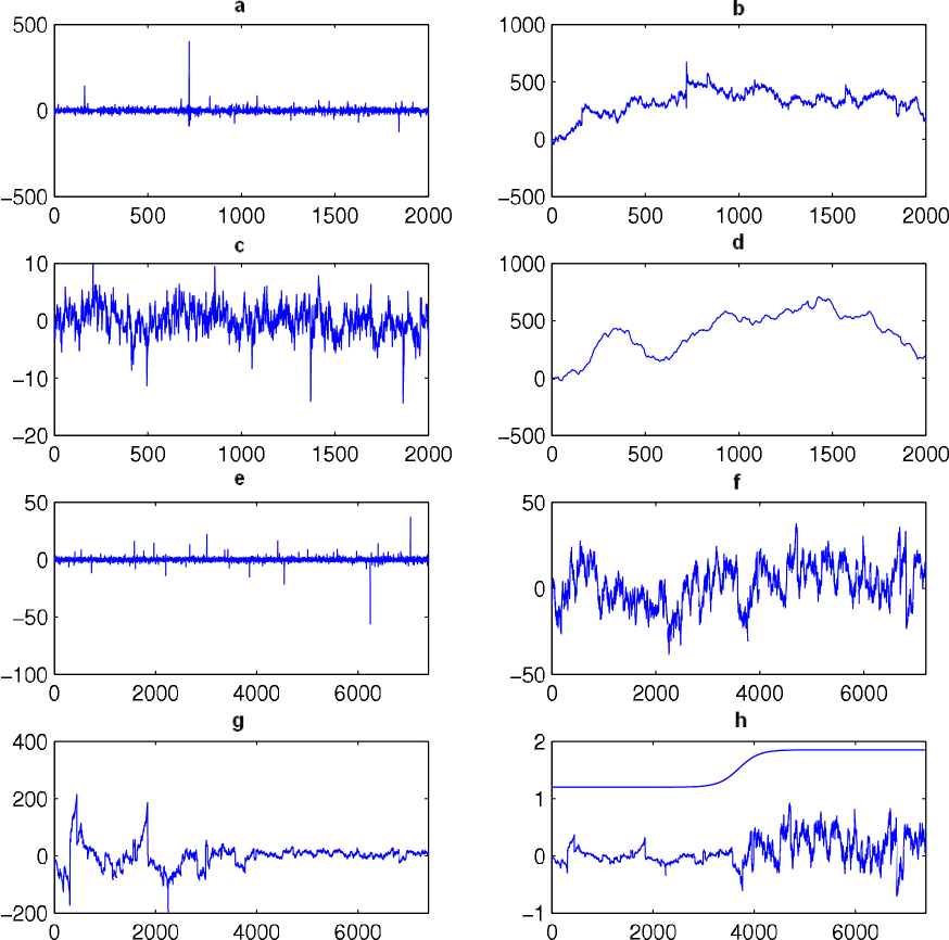
Figure 1: Paths of localisable processes. (a) The process in Example 3.4 and (b) the integrated version. (c) The process in Example 3.3 and (d) the integrated version. (e) Reverse Ornstein-Uhlenbeck processes with $\lambda=1$, and (f) $\lambda=0.01$. (g) A multistable reverse Ornstein-Uhlenbeck process with $\lambda=0.01$ and (h) the renormalised version along with $\alpha(t)$.

References

• [1] Cohen, S. and Lacaux, C. and Ledoux, M. (2008). A general framework for simulation of fractional fields. Stochastic Process. Appl., (118) 9, 1489 1517.
• [2] Cohen, S. (1999) From self-similarity to local self-similarity: the estimation problem, Fractal in Engineering, J. Lévy Véhel, E. Lutton and C. Tricot (eds.), Springer Verlag.
• [3] Falconer, K.J. (2002). Tangent fields and the local structure of random fields. J. Theoret. Probab. 15, 731–750.
• [4] Falconer, K.J. (2003). The local structure of random processes. J. London Math. Soc.(2) 67, 657–672.
• [5] Falconer, K.J. and Lévy Véhel, J. (2008). Multifractional, multistable, and other processes with prescribed local form, J. Theoret. Probab., DOI 10.1007/s10959-008-0147-9.
• [6] Kingman, J.F.C. (1993). Poisson Processes, Oxford University Press, Oxford.
• [7] Lévy Véhel, J. and Seuret, S. (2004). The 2-microlocal Formalism, Fractal Geometry and Applications: A Jubilee of Benoit Mandelbrot, Proc. Sympos. Pure Math., 72 (2), 153-215.
• [8] Negoro, A. (1994). Stable-like processes: construction of the transition density and the behavior of sample paths near t = 0. Osaka J. Math. (31) 1, 189- 214.
• [9] Rogers, L.C.G. and Williams, D. (2000). Diffusions, Markov Processes and Martingales, Volume 1, 2nd edn. Cambridge University Press, Cambridge.
• [10] Samorodnitsky, G. and Taqqu, M.S. (1994) Stable Non-Gaussian Random Processes, Chapman and Hall.
• [11] Sato, K. (1999). Lévy Processes and Infinitely Divisible Distributions, Cambridge University Press, Cambridge.
• [12] Stoev, S. and Taqqu, M.S. (2004). Simulation methods for linear fractional stable motion and FARIMA using the Fast Fourier Transform. Fractals (2) 1,95–121.
• [13] Titchmarsh, E. (1948) Introduction to the Theory of Fourier Integrals, Second Edition, Clarendon Press.
Refer to caption