Supersymmetric models with minimal flavour violation and their running

Abstract

We revisit the formulation of the principle of minimal flavor violation (MFV) in the minimal supersymmetric extension of the standard model, both at moderate and large $\tan\beta$, and with or without new CP-violating phases. We introduce a counting rule which keeps track of the highly hierarchical structure of the Yukawa matrices. In this manner, we are able to control systematically which terms can be discarded in the soft SUSY breaking part of the Lagrangian. We argue that for the implementation of this counting rule, it is convenient to introduce a new basis of matrices in which both the squark (and slepton) mass terms as well as the trilinear couplings can be expanded. We derive the RGE for the MFV parameters and show that the beta functions also respect the counting rule. For moderate $\tan\beta$, we provide explicit analytic solutions of these RGE and illustrate their behaviour by analyzing the neighbourhood (also switching on new phases) of the SPS-1a benchmark point. We then show that even in the case of large $\tan\beta$, the RGE remain valid and that the analytic solutions obtained for moderate $\tan\beta$ still allow us to understand the most important features of the running of the parameters, as illustrated with the help of the SPS-4 benchmark point.

1 Introduction

In the Standard Model, renormalizability restricts the possible sources of flavour violations to only one matrix, the Cabibbo-Kobayashi-Maskawa (CKM) matrix. Its almost diagonal structure (like the values of all the other free parameters of the model) remains unexplained.

In extensions of the Standard Model, as soon as new degrees of freedom appear, the possibilities to generate transitions among flavours increase very rapidly, and may give rise to a richer phenomenology than what the Standard Model alone would allow. The wealth of recent experimental results produced at kaon and $B$ factories shows, however, that if new degrees of freedom exist just above the electroweak symmetry breaking scale, their influence on low-energy flavour physics is smaller than one would naively expect, below the current experimental sensitivity. This imposes a nontrivial constraint for model building, and forces one to impose some sort of protection against flavour violations.

A convenient way to do this, without excluding completely the possibility to have new effects in flavour physics, is the principle of minimal flavour violation (MFV) [1, 2] (see also Ref. [3]). According to this, even in extensions of the Standard Model, the only source of flavour violations is in the Yukawa matrices, and since one of them can always be diagonalized, in the CKM matrix. In its latest, more complete implementation, the principle is formulated as a symmetry: one starts from the observation that the large global flavour symmetry group of the Standard Model in the absence of the Yukawa couplings is saved even in their presence if they are promoted to the status of spurions, i.e. if they are assigned transformation properties under the flavour group. The principle of MFV requires that the same symmetry holds even in extensions of the Standard Model – the only allowed spurions being the Yukawa matrices.

In this paper, we concentrate on supersymmetric extensions of the Standard Model with minimal field content and exact R-parity (MSSM) (for a nice introduction, cf. Ref. [4]) and discuss the principle of MFV within this framework. Our main points are:

1. We observe that, if one considers the Yukawa matrices as dimension-zero spurions, and allows any power of them to appear in local operators, imposing MFV on the MSSM does not restrict the number of free parameters of the model, but amounts to a mere reparametrization. Still, if one requires that the coupling constant of the model are of order one, some of them are irrelevant for the phenomenology and can therefore be dropped.

2. In order to decide systematically which terms are irrelevant and which ones should be kept, we find it convenient to introduce a counting rule, and use as expansion parameter $\lambda$, the Cabibbo angle. We use this expansion parameter to take into account not only the highly hierarchical CKM matrix, but also the highly hierarchical quark and lepton masses. Each of the MFV parameters will therefore be assigned an order in $\lambda$ – once one has set the accuracy of its calculation to a certain level, $\mathcal{O}(\lambda^{n})$, it is immediate to see which MFV parameters should be kept.

3. Since imposing MFV amounts to a mere reparametrization of the generic MSSM, it is obvious that the principle is renormalization group (RG) invariant – what is not guaranteed is that the coefficients will keep their order in $\lambda$ during the running. We will rewrite the renormalization group equations (RGE) in MFV form, checking that the beta functions also respect the same counting rules as the parameters themselves. As such, this is only a necessary, but not yet sufficient condition to prove that the MFV principle is truly RGE invariant. We will therefore study the solutions of the RGE numerically, and show that indeed they respect the counting rules when evolving from the high to the low scale – none of the irrelevant parameters at the high scale may become so large during the RG evolution that it becomes of phenomenological importance at the low scale. We will also show that the converse is not true: generic MFV-like boundary conditions at the low scale will not necessarily evolve to a MFV-like MSSM at the high scale. Therefore, the assumption that the MFV hypothesis in the MSSM is valid at different scales makes it even more restrictive at the low scale.

4. We discuss in detail the possible new CP-violating phases allowed by the MFV hypothesis, and analyze their behaviour under the running. We show that they tend to vanish at the low scale – how fast they do that depends on the initial conditions at the high scale.

While this paper was being completed, a preprint appeared which also analyzes the behaviour of MFV models under running [5]. There, the numerical analysis is performed with the help of SOFTSUSY [6], one of the available codes which allow one to run the MSSM with a generic flavour structure according to the full RGE to two loops. In this paper, the authors start with MFV-compatible initial conditions at the GUT scale, evolve all the parameters down to the electroweak scale, and project back the model on the MFV parameters, with the help of a fit. Their analysis is valid for moderate $\tan\beta$, and only for real MFV coefficients. In this manner, they find out that the MFV parameters have quasi fixed points at the low scale. We will confirm their finding, and also provide an analytical explanation for this behaviour. Furher, we will perform the analysis also for large $\tan\beta$, and in the presence of new CP-violating phases in the MFV expansions.

2 Revisiting minimal flavour violation

2.1 Definition of minimal flavour violation

Gauge interactions in the Standard Model are flavour blind. If one sets the Yukawa matrices to zero, the Standard Model becomes invariant under a large global symmetry group $G_{F}\sim[U(3)]^{5}$ [7]:

$$G_{F}\equiv G_{q}\otimes G_{\ell}\otimes U(1)_{B}\otimes U(1)_{L}\otimes U(1)_{Y}\otimes U(1)_{PQ}\otimes U(1)_{E_{R}}\;,$$ (1)

where

$$G_{q}\equiv SU(3)_{Q_{L}}\otimes SU(3)_{U_{R}}\otimes SU(3)_{D_{R}}\;,\quad G_{\ell}\equiv SU(3)_{L_{L}}\otimes SU(3)_{E_{R}}\;\;.$$ (2)

The five $U(1)$ factors have been decomposed in the three which remain a symmetry even in the presence of Yukawa interactions (related to baryon and lepton number and hypercharge), and the remaining two. Following Ref. [2], we write these as a phase transformation affecting $D_{R}$ and $E_{R}$ at the same time, the Peccei-Quinn symmetry of the two-Higgs doublet model (denoted here by $U(1)_{PQ}$) and one affecting only $E_{R}$.

The Yukawa matrices break $G_{q}\otimes G_{\ell}\otimes U(1)_{PQ}\otimes U(1)_{E_{R}}$:

$$\mathcal{L}_{\scriptscriptstyle Y}=\bar{U}_{R}\,\mathbf{Y}_{u}\,Q_{L}H+\bar{D}_{R}\,\mathbf{Y}_{d}\,Q_{L}H_{c}+E_{R}\,\mathbf{Y}_{e}\,L_{L}H_{c}+\mathrm{h.c.}\;\;,$$ (3)

where $H_{c}=i\tau_{2}H^{\ast}$. As observed in Ref. [2], the Standard Model remains formally invariant under $G_{q}\otimes G_{\ell}$ in the presence of the Yukawa matrices if these are promoted to spurion fields transforming as

$$\mathbf{Y}_{u}\sim(\bar{3},3,1)\;,\quad\mathbf{Y}_{d}\sim(\bar{3},1,3)\quad\mbox{under }G_{q}\;,$$ (4)

and

$$\mathbf{Y}_{e}\sim(\bar{3},3)\quad\mbox{under }G_{\ell}\;\;.$$ (5)

The symmetry is broken whenever the Yukawa matrices are frozen at a certain value – on the other hand, different forms of the Yukawa matrices which are related by $G_{q}$ and $G_{\ell}$ transformations are physically equivalent. In what follows, we will choose the following background values

$$\mathbf{Y}_{u}=\lambda_{u}V\;,\quad\mathbf{Y}_{d}=\lambda_{d}\;,\quad\mathbf{Y}_{e}=\lambda_{e}\;,$$ (6)

where $\lambda_{u}=\mathrm{diag}(y_{u},y_{c},y_{t})$, $\lambda_{d}=\mathrm{diag}(y_{d},y_{s},y_{b})$ and $\lambda_{e}=\mathrm{diag}(y_{e},y_{\mu},y_{\tau})$, and $V$ is the CKM matrix.

An extension of the Standard Model is said to respect MFV if it is symmetric under $G_{q}\otimes G_{\ell}$ in the presence of Yukawa spurions. While new matter fields in such an extension are of course allowed, one is not supposed to introduce new spurion fields beyond the Yukawa matrices.

2.2 MFV in the MSSM: a reparametrization of the soft SUSY breaking terms

In a supersymmetric extension of the Standard Model, the superpotential automatically satisfy the MFV principle. On the other hand, MFV strongly constrains the soft supersymmetry breaking terms. We will illustrate this statement by considering the mass term for the left-handed squarks

$$\mathcal{L}_{\mathbf{m}_{Q}^{2}}\equiv-\tilde{Q}^{\dagger}\mathbf{m}_{Q}^{2}\cdot\tilde{Q}\;\;,$$ (7)

and showing first that MFV amounts in principle to a reparametrization of a generic hermitian $3\times 3$ matrix, and later that if one excludes the possibility of having enormous coupling constants, MFV is indeed quite constraining. MFV requires this term to become formally invariant under $G_{q}$, hence it must transform like $(8,1,1)$. Since we are not allowed to introduce new spurions, we have to obtain this transformation property with the help of the Yukawa matrices, as with terms like $\mathbf{Y}_{u}^{\dagger}\mathbf{Y}_{u}$ or $\mathbf{Y}_{d}^{\dagger}\mathbf{Y}_{d}$. Moreover, one can construct invariants under $G_{q}$ also with the help of $\epsilon$-tensors. Such terms have recently been systematically studied in Ref. [8], and permit to extend the MFV principle to the R-parity violating interactions. Interestingly, MFV alone is then sufficient to prevent the proton from decaying too rapidly – a fact which lends additional support to the validity of the MFV hypothesis at low energy.

For the R-parity conserving sector of the MSSM, on which we concentrate in the present paper, these $\epsilon$-tensor terms have been shown to be very suppressed [8]. Hence, ignoring them altogether, MFV permits to write $\mathbf{m}_{Q}^{2}$ as the infinite sum:

$$\mathbf{m}_{Q}^{2}=a_{1}\mathbf{1}+b_{1}\mathbf{Y}_{u}^{\dagger}\mathbf{Y}_{u}+b_{2}\mathbf{Y}_{d}^{\dagger}\mathbf{Y}_{d}+c_{1}\mathbf{Y}_{u}^{\dagger}\mathbf{Y}_{u}\mathbf{Y}_{u}^{\dagger}\mathbf{Y}_{u}+c_{2}\mathbf{Y}_{d}^{\dagger}\mathbf{Y}_{d}\mathbf{Y}_{d}^{\dagger}\mathbf{Y}_{d}+\ldots$$ (8)

Actually, the infinite sum collapses on its first few terms: the Yukawa couplings are $3\times 3$ matrices, hence they respect the corresponding Cayley-Hamilton identities. The hermitian matrix $\mathbf{m}_{Q}^{2}$ does not contain more than nine independent real parameters and it can be shown that the sum in Eq. (8) spans the space of hermitian matrices [9].

The Cayley-Hamilton identities read for $3\times 3$ matrices

$$\mathbf{X}^{3}-\left\langle\mathbf{X}\right\rangle\mathbf{X}^{2}+\frac{1}{2}\mathbf{X}\left(\left\langle\mathbf{X}\right\rangle^{2}-\left\langle\mathbf{X}^{2}\right\rangle\right)-\det\mathbf{X}=0\;,$$ (9)

and can be rewritten in terms of traces only if the determinant is expressed as

$$\det\mathbf{X}=\frac{1}{3}\left\langle\mathbf{X}^{3}\right\rangle-\frac{1}{2}\left\langle\mathbf{X}\right\rangle\left\langle\mathbf{X}^{2}\right\rangle+\frac{1}{6}\left\langle\mathbf{X}\right\rangle^{3}\;\;.$$ (10)

In other words, all powers of three or more of a combination of Yukawa matrices, $\mathbf{X}^{n>2}$, can be eliminated in terms of only $\mathbf{X}^{2},\mathbf{X},\mathbf{1}$, with coefficients involving the trace of $\mathbf{X}^{2}$ and $\mathbf{X}$. Further, identities involving two (or more) different combinations, $\mathbf{A}$ and $\mathbf{B}$ say, can be found by substituting $\mathbf{X}=a\mathbf{A}+b\mathbf{B}$ in Eq. (9) and extracting a given power of $a$ and $b$. For example, a relevant identity is

$$\!\!\!\!\!\!\mathbf{A}^{2}\mathbf{B}+\mathbf{ABA}+\mathbf{BA}^{2}=\mathbf{A}^{2}\left\langle\mathbf{B}\right\rangle+\left(\mathbf{AB}+\mathbf{BA}\right)\left\langle\mathbf{A}\right\rangle+\mathbf{A}\left(\left\langle\mathbf{AB}\right\rangle-\left\langle\mathbf{A}\right\rangle\left\langle\mathbf{B}\right\rangle\right)$$

$$\!\!\!\!\!\!+\frac{1}{2}\mathbf{B}\left(\left\langle\mathbf{A}^{2}\right\rangle-\left\langle\mathbf{A}\right\rangle^{2}\right)+\frac{1}{2}\left\langle\mathbf{B}\right\rangle\left(\left\langle\mathbf{A}\right\rangle^{2}-\left\langle\mathbf{A}^{2}\right\rangle\right)+\left\langle\mathbf{A}^{2}\mathbf{B}\right\rangle-\left\langle\mathbf{A}\right\rangle\left\langle\mathbf{AB}\right\rangle\;,$$ (11)

with $\mathbf{A}=\mathbf{Y}_{u}^{\dagger}\mathbf{Y}_{u}$ and $\mathbf{B}=\mathbf{Y}_{d}^{\dagger}\mathbf{Y}_{d}$.

Taking into account these identities, the most general expression for $\mathbf{m}_{Q}^{2}$ respecting MFV becomes

$$\mathbf{m}_{Q}^{2} =z_{1}\mathbf{1}+z_{2}\mathbf{Y}_{u}^{\dagger}\mathbf{Y}_{u}+z_{3}\mathbf{Y}_{d}^{\dagger}\mathbf{Y}_{d}+z_{4}(\mathbf{Y}_{u}^{\dagger}\mathbf{Y}_{u})^{2}+z_{5}(\mathbf{Y}_{d}^{\dagger}\mathbf{Y}_{d})^{2}$$

$$+z_{6}\left(\mathbf{Y}_{d}^{\dagger}\mathbf{Y}_{d}\mathbf{Y}_{u}^{\dagger}\mathbf{Y}_{u}+\mathrm{h.c.}\right)+z_{7}\mathbf{Y}_{u}^{\dagger}\mathbf{Y}_{u}\mathbf{Y}_{d}^{\dagger}\mathbf{Y}_{d}\mathbf{Y}_{u}^{\dagger}\mathbf{Y}_{u}$$

$$+z_{8}\mathbf{Y}_{d}^{\dagger}\mathbf{Y}_{d}\mathbf{Y}_{u}^{\dagger}\mathbf{Y}_{u}\mathbf{Y}_{d}^{\dagger}\mathbf{Y}_{d}+z_{9}\left((\mathbf{Y}_{u}^{\dagger}\mathbf{Y}_{u})^{2}(\mathbf{Y}_{d}^{\dagger}\mathbf{Y}_{d})^{2}+\mathrm{h.c.}\right)$$

$$+iz_{10}(\mathbf{Y}_{d}^{\dagger}\mathbf{Y}_{d}\mathbf{Y}_{u}^{\dagger}\mathbf{Y}_{u}-\mathrm{h.c.})+iz_{11}\left((\mathbf{Y}_{u}^{\dagger}\mathbf{Y}_{u})^{2}\mathbf{Y}_{d}^{\dagger}\mathbf{Y}_{d}-\mathrm{h.c.}\right)$$

$$+iz_{12}\left((\mathbf{Y}_{d}^{\dagger}\mathbf{Y}_{d})^{2}\mathbf{Y}_{u}^{\dagger}\mathbf{Y}_{u}-\mathrm{h.c.}\right)+iz_{13}\left((\mathbf{Y}_{u}^{\dagger}\mathbf{Y}_{u})^{2}(\mathbf{Y}_{d}^{\dagger}\mathbf{Y}_{d})^{2}-\mathrm{h.c.}\right)$$

$$+iz_{14}\left(\mathbf{Y}_{u}^{\dagger}\mathbf{Y}_{u}\mathbf{Y}_{d}^{\dagger}\mathbf{Y}_{d}(\mathbf{Y}_{u}^{\dagger}\mathbf{Y}_{u})^{2}-\mathrm{h.c.}\right)+iz_{15}\left(\mathbf{Y}_{d}^{\dagger}\mathbf{Y}_{d}\mathbf{Y}_{u}^{\dagger}\mathbf{Y}_{u}(\mathbf{Y}_{d}^{\dagger}\mathbf{Y}_{d})^{2}-\mathrm{h.c.}\right)$$

$$+iz_{16}\left(\mathbf{Y}_{u}^{\dagger}\mathbf{Y}_{u}(\mathbf{Y}_{d}^{\dagger}\mathbf{Y}_{d})^{2}(\mathbf{Y}_{u}^{\dagger}\mathbf{Y}_{u})^{2}-\mathrm{h.c.}\right)+iz_{17}\left(\mathbf{Y}_{d}^{\dagger}\mathbf{Y}_{d}(\mathbf{Y}_{u}^{\dagger}\mathbf{Y}_{u})^{2}(\mathbf{Y}_{d}^{\dagger}\mathbf{Y}_{d})^{2}-\mathrm{h.c.}\right)\;\;,$$ (12)

with the $z_{i}$ being real parameters. A generic $3\times 3$ hermitian matrix can be described by nine real constants – in Eq. (12), $\mathbf{m}_{Q}^{2}$ is expressed in terms of seventeen real constants, so that eight of them must be linearly dependent. Even if we do not specify the linear relations which allow one to eliminate eight of these constants, it is clear that MFV amounts to a mere reparametrization of the soft SUSY-breaking terms of the MSSM, since the original expansion in Eq. (8) contains a basis and the Cayley-Hamilton relations are exact. A similar argument can be used also for all other terms.

What is special about the MFV parametrization is that if all the $z_{i}$’s are of the same order of magnitude, the structure of $\mathbf{m}_{Q}^{2}$ is highly non-generic. Conversely, if one writes down a generic $\mathbf{m}_{Q}^{2}$ matrix and projects it on the MFV basis, the coefficients $z_{i}$ so obtained will typically span many orders of magnitude. We define extensions of the Standard Model respecting MFV by the additional requirement that the coefficients appearing in front of the various MFV terms are of the same order of magnitude.

2.3 Counting rules and a new basis

If one takes all the $z_{i}$ coefficients to be of the same order of magnitude, several of the terms in Eq. (12) (and in the analogous ones for the other soft SUSY-breaking terms) can be disposed of. In this subsection, we will discuss how to do this in a systematic way, and will argue that it is more convenient to change basis in order to work with MFV. For example, taking into account the actual values of the Yukawa coefficients of the up, charm and top quarks, we conclude that the two matrices

$$\left(\mathbf{Y}_{u}^{\dagger}\mathbf{Y}_{u}\right)^{2}=V^{\dagger}\lambda_{u}^{4}V\;,\qquad\mathbf{Y}_{u}^{\dagger}\mathbf{Y}_{u}=V^{\dagger}\lambda_{u}^{2}V$$ (13)

are proportional to each other up to a correction of relative order $\mathcal{O}(y_{c}^{2}/y_{t}^{2})$,

$$\left(\mathbf{Y}_{u}^{\dagger}\mathbf{Y}_{u}\right)^{2}-y_{t}^{2}\mathbf{Y}_{u}^{\dagger}\mathbf{Y}_{u}=y_{t}^{2}y_{c}^{2}V_{2i}^{\ast}V_{2j}+\mathcal{O}(y_{c}^{4})\;,$$ (14)

which is usually neglected since $y_{c}^{2}\ll 1$. A similar argument can be applied to $\mathbf{Y}_{d}^{\dagger}\mathbf{Y}_{d}$, since $y_{s}^{2}\ll 1$ also. We will therefore never include any power of $\mathbf{Y}_{u}^{\dagger}\mathbf{Y}_{u}$ or $\mathbf{Y}_{d}^{\dagger}\mathbf{Y}_{d}$ in our analysis, and keep the latter to allow $\tan\beta$ to be large (remember that the two Higgs doublets of the MSSM separately give mass to the up and down-quarks: $v_{u}\lambda_{u}=diag(m_{u},m_{c},m_{t})$ and $v_{d}\lambda_{d}=diag(m_{d},m_{s},m_{b})$, with $v_{u,d}$ the two Higgs vacuum expectation values, and $\tan\beta\equiv v_{u}/v_{d}$). With this approximation, the MFV version of the soft SUSY-breaking terms reads

$$\mathbf{m}_{Q}^{2} =m_{0}^{2}\left[a_{1}+b_{1}\mathbf{Y}_{u}^{\dagger}\mathbf{Y}_{u}+b_{2}\mathbf{Y}_{d}^{\dagger}\mathbf{Y}_{d}+(b_{3}\mathbf{Y}_{d}^{\dagger}\mathbf{Y}_{d}\mathbf{Y}_{u}^{\dagger}\mathbf{Y}_{u}+\mathrm{h.c.})\right]\;,$$

$$\mathbf{m}_{U}^{2} =m_{0}^{2}\left[a_{2}+\mathbf{Y}_{u}\!\left(b_{5}+c_{1}\mathbf{Y}_{u}^{\dagger}\mathbf{Y}_{u}+c_{2}\mathbf{Y}_{d}^{\dagger}\mathbf{Y}_{d}+(c_{3}\mathbf{Y}_{d}^{\dagger}\mathbf{Y}_{d}\mathbf{Y}_{u}^{\dagger}\mathbf{Y}_{u}+\mathrm{h.c.})\right)\!\mathbf{Y}_{u}^{\dagger}\right]\;,$$

$$\mathbf{m}_{D}^{2} =m_{0}^{2}\left[a_{3}+\mathbf{Y}_{d}\!\left(b_{6}+c_{4}\mathbf{Y}_{u}^{\dagger}\mathbf{Y}_{u}+c_{5}\mathbf{Y}_{d}^{\dagger}\mathbf{Y}_{d}+(c_{6}\mathbf{Y}_{d}^{\dagger}\mathbf{Y}_{d}\mathbf{Y}_{u}^{\dagger}\mathbf{Y}_{u}+\mathrm{h.c.})\right)\!\mathbf{Y}_{d}^{\dagger}\right]\;,$$

$$\mathbf{A}^{U} =A_{0}\mathbf{Y}_{u}\!\left(a_{4}+b_{7}\mathbf{Y}_{d}^{\dagger}\mathbf{Y}_{d}+c_{7}\mathbf{Y}_{u}^{\dagger}\mathbf{Y}_{u}+c_{8}\mathbf{Y}_{d}^{\dagger}\mathbf{Y}_{d}\mathbf{Y}_{u}^{\dagger}\mathbf{Y}_{u}+c_{9}\mathbf{Y}_{u}^{\dagger}\mathbf{Y}_{u}\mathbf{Y}_{d}^{\dagger}\mathbf{Y}_{d}\right)\;,$$

$$\mathbf{A}^{D} =A_{0}\mathbf{Y}_{d}\!\left(a_{5}+b_{8}\mathbf{Y}_{u}^{\dagger}\mathbf{Y}_{u}+c_{10}\mathbf{Y}_{d}^{\dagger}\mathbf{Y}_{d}+c_{11}\mathbf{Y}_{d}^{\dagger}\mathbf{Y}_{d}\mathbf{Y}_{u}^{\dagger}\mathbf{Y}_{u}+c_{12}\mathbf{Y}_{u}^{\dagger}\mathbf{Y}_{u}\mathbf{Y}_{d}^{\dagger}\mathbf{Y}_{d}\right)\;.$$ (15)

Until now, we have used only the fact that the Yukawa matrices are highly hierarchical along their diagonal. They are, however, also hierarchical in their off-diagonal structure, and taking this into account leads to further simplifications. In order to do this in a systematic way, we use as expansion parameter the Cabibbo angle $\lambda=0.23$, which appears in the Wolfenstein parametrization of the CKM matrix as follows (to leading order in $\lambda$ – in subsequent calculations we will always include higher orders also)

$$V\approx\left(\begin{array}[c]{ccc}1&\lambda&A\lambda^{3}\left(\rho-i\eta\right)\\ -\lambda&1&A\lambda^{2}\\ A\lambda^{3}\left(1-\rho-i\eta\right)&-A\lambda^{2}&1\end{array}\right)\;,$$ (16)

We then adopt the following counting conventions for the quark mass ratios at the electroweak scale $\mu=M_{Z}$:

$$\frac{m_{u}}{m_{t}}\sim\mathcal{O}(\lambda^{7}),\;\;\frac{m_{c}}{m_{t}}\sim\mathcal{O}(\lambda^{4}),\;\;y_{t}\sim\mathcal{O}(1)\;,$$ (17)

$$\frac{m_{d}}{m_{t}}\sim\mathcal{O}(\lambda^{7}),\;\;\frac{m_{s}}{m_{t}}\sim\mathcal{O}(\lambda^{5}),\;\;\frac{m_{b}}{m_{t}}\sim\mathcal{O}(\lambda^{3})\;.$$

For example, the difference in Eq. (14),

$$\mathbf{Y}_{u}^{\dagger}\mathbf{Y}_{u}\mathbf{Y}_{u}^{\dagger}\mathbf{Y}_{u}-y_{t}^{2}\mathbf{Y}_{u}^{\dagger}\mathbf{Y}_{u}=\left(\begin{array}[c]{ccc}\mathcal{O}\left(\lambda^{8}\right)&\mathcal{O}\left(\lambda^{7}\right)&\mathcal{O}\left(\lambda^{9}\right)\\ \mathcal{O}\left(\lambda^{7}\right)&\mathcal{O}\left(\lambda^{6}\right)&\mathcal{O}\left(\lambda^{8}\right)\\ \mathcal{O}\left(\lambda^{9}\right)&\mathcal{O}\left(\lambda^{8}\right)&\mathcal{O}\left(\lambda^{10}\right)\end{array}\right)\;,$$ (18)

represents a correction of at least $\mathcal{O}(\lambda^{2})$ (in every entry) to each of the two terms, cf.

$$\mathbf{Y}_{u}^{\dagger}\mathbf{Y}_{u}=\left(\begin{array}[c]{ccc}\mathcal{O}\left(\lambda^{6}\right)&\mathcal{O}\left(\lambda^{5}\right)&\mathcal{O}\left(\lambda^{3}\right)\\ \mathcal{O}\left(\lambda^{5}\right)&\mathcal{O}\left(\lambda^{4}\right)&\mathcal{O}\left(\lambda^{2}\right)\\ \mathcal{O}\left(\lambda^{3}\right)&\mathcal{O}\left(\lambda^{2}\right)&\mathcal{O}\left(1\right)\end{array}\right)\;\;.$$ (19)

This shows that while MFV can indeed be viewed as a reparametrization, cf. Eq. (12), it is on the other hand a very special one, because the basis in the linear space of $3\times 3$ hermitian matrices on which $m_{Q}^{2}$ is projected is almost a singular one. Several of the basis vectors are almost parallel to each other, and their difference is tiny in comparison to either of the vectors. Since our aim here is to link the MFV concept to a counting rule, and define clearly which terms should be kept and which should be neglected, it is a lot more convenient to use a basis of vectors which are as little aligned to each other as possible. In this way, contributions which are small and may (or may not) be neglected will not have to be searched for in small differences between similar contributions, but will be clearly identified and separated from the rest. In order to illustrate this concept, we come back to Eq. (14) and observe that the large piece in both $\mathbf{Y}_{u}^{\dagger}\mathbf{Y}_{u}$ and its square is proportional to the matrix $V_{3i}^{\ast}V_{3j}$, whereas the small one, as indicated in Eq. (14) is proportional to $V_{2i}^{\ast}V_{2j}$. So, instead of using $\mathbf{Y}_{u}^{\dagger}\mathbf{Y}_{u}$ and $(\mathbf{Y}_{u}^{\dagger}\mathbf{Y}_{u})^{2}$ as basis vectors, and allow both to have coefficients of order one, we find it more convenient to use $V_{3i}^{\ast}V_{3j}$ and $V_{2i}^{\ast}V_{2j}$, and say that the first can have a coefficient of order one, but the latter should have it of order $y_{c}^{2}\sim\lambda^{8}$, and (depending on where one sets its accuracy) can therefore be neglected.

If we follow the same logic for $\mathbf{Y}_{d}^{\dagger}\mathbf{Y}_{d}$ and its square, we find that in this case we should rather use as basis vectors the matrices $\delta_{i3}\delta_{j3}$ and $\delta_{i2}\delta_{j2}$, and that the coefficients of these terms should be of order $y_{b}^{2}$ and $y_{s}^{2}$ respectively (how to translate this into a power of $\lambda$ depends on $\tan\beta$). Taking into account all the possible structures which can emerge, and which can all be multiplied with each other, we are led to consider a set of sixteen matrices, which form a closed algebra under multiplication:

$$\begin{array}[c]{llll}X_{1}=\delta_{3i}\delta_{3j}&X_{5}=\delta_{3i}V_{3j}&X_{9}=V_{3i}^{\ast}\delta_{3j}&X_{13}=V_{3i}^{\ast}V_{3j}\\ X_{2}=\delta_{2i}\delta_{2j}&X_{6}=\delta_{2i}V_{2j}&X_{10}=V_{2i}^{\ast}\delta_{2j}&X_{14}=V_{2i}^{\ast}V_{2j}\\ X_{3}=\delta_{3i}\delta_{2j}&X_{7}=\delta_{3i}V_{2j}&X_{11}=V_{3i}^{\ast}\delta_{2j}&X_{15}=V_{3i}^{\ast}V_{2j}\\ X_{4}=\delta_{2i}\delta_{3j}&X_{8}=\delta_{2i}V_{3j}&X_{12}=V_{2i}^{\ast}\delta_{3j}&X_{16}=V_{2i}^{\ast}V_{3j}\end{array}$$ (20)

Notice that all these matrices have at least one entry (almost) equal to one, so that they can all be counted as of order one.

If we now write Eq. (15) (or even start from the earlier stage given by Eq. (12)) in this basis and assume that all $a_{i}$, $b_{i}$ and $c_{i}$ coefficients are of order one, we can immediately read out the size of the coefficients in front of the $X_{i}$ matrices and decide which one to keep and which not. In particular, if we drop terms of order $\lambda^{6}\sim 10^{-4}$ and higher, we can reduce the soft SUSY-breaking terms to the following

$$\mathbf{m}_{Q}^{2} =\tilde{a}_{1}+x_{1}X_{13}+y_{1}X_{1}+y_{2}X_{5}+y_{2}^{\ast}X_{9}\;,$$

$$\mathbf{m}_{U}^{2} =\tilde{a}_{2}+x_{2}X_{1}\;,$$

$$\mathbf{m}_{D}^{2} =\tilde{a}_{3}+y_{3}X_{1}+w_{1}X_{3}+w_{1}^{\ast}X_{4}\;,$$

$$\mathbf{A}^{U} =\tilde{a}_{4}X_{5}+y_{4}X_{1}+w_{2}X_{6}\;,$$

$$\mathbf{A}^{D} =\tilde{a}_{5}X_{1}+y_{5}X_{5}+w_{3}X_{2}+w_{4}X_{4}\;,$$ (21)

where, for simplicity, we have absorbed the overall scales $m_{0}^{2}$ and $A_{0}$ into the coefficients. Since the matrices $X_{i}$ are all of order one, the coefficients now carry the order in $\lambda$, and we have reflected this in the symbols which identify them. Relative to the leading terms, the two $x_{i}$’s are of order one, $\tilde{a}_{5}$ (which now incorporates $y_{b}$ – while $\tilde{a}_{4}$ incorporates $y_{t}$), as well as the $y_{i}$’s can become of order one if $\tan\beta\sim\lambda^{-3}$, and the $w_{i}$’s are suppressed by at least two powers of $\lambda$, even when $\tan\beta\sim\lambda^{-3}$. More specifically:

$$\frac{\tilde{a}_{5}}{\tilde{a}_{4}}\sim\frac{y_{5}}{\tilde{a}_{4}}\sim\mathcal{O}(\lambda^{3}t_{\beta})\;,\;\;\;\;\;\;\;\;\frac{y_{1,2}}{\tilde{a}_{1}}\sim\frac{y_{3}}{\tilde{a}_{3}}\sim\frac{y_{4}}{\tilde{a}_{4}}\sim\mathcal{O}(\lambda^{6}t_{\beta}^{2})\;,$$

$$\frac{w_{1}}{\tilde{a}_{3}}\sim\mathcal{O}(\lambda^{10}t_{\beta}^{2})\;,\;\;\;\frac{w_{2}}{\tilde{a}_{3}}\sim\mathcal{O}(\lambda^{4})\;,\;\;\;\frac{w_{3}}{\tilde{a}_{5}}\sim\mathcal{O}(\lambda^{2})\;,\;\;\;\frac{w_{4}}{\tilde{a}_{5}}\sim\mathcal{O}(\lambda^{4})\;.$$ (22)

We stress that this representation remains valid even in the case of large $\tan\beta$, up to $\tan\beta\sim\mathcal{O}(m_{t}/m_{b})$ – on the other hand, if the latter is not large, all the $y_{1-4}$, $w_{1}$ and $w_{4}$ can be dropped. Also, $a_{1-3}$, $x_{1}$, $x_{2}$, $y_{1}$ and $y_{3}$ must be real since $\mathbf{m}_{Q,U,D}^{2}$ are hermitian, while all the others can be complex. There are thus a priori nine new CP-violating phases entering in the squark soft-breaking terms, though only those of $\tilde{a}_{4}$ and (less so) $\tilde{a}_{5}$ and $y_{5}$ are unsuppressed for moderate $\tan\beta$.

Looking at the representation (21), one may observe that, in contrast to the original formulation of Ref. [2], the symmetry principle which is behind MFV is not immediately visible anymore. Actually, the essential concept that the only source of flavour violation is the CKM matrix is still manifest in the $X_{i}$ basis, and moreover:

1. The symmetry principle which forms the basis of MFV is used once and for all, and leads to the basis shown, e.g. in Eq. (12). The relation between the standard MFV and the $X_{i}$ basis can also be derived once and for all; it is given explicitly in Appendix B in terms of the running Yukawa couplings, to be defined in Sect. 3.

2. To make the most of the MFV principle, one still has to drop suppressed terms in the most general representation provided by MFV in Eq. (15). As we have discussed above, it is easier and more transparent to do so in the $X_{i}$ basis.

3. The $x_{i}$ coefficients have a direct, simple relation to the mass insertions [10], which are useful for phenomenological studies of flavour violations, as we will discuss in detail in the next section.

4. The scalings of the $x_{i}$ coefficients, as well as the decompositions (21), are stable under the RGE’s, as will be discussed in details in Sect. 3. Further, the formulation of the RGE’s for the $x_{i}$ coefficients is particularly convenient, especially because one can immediately see the order of the different terms appearing in their beta functions.

2.4 MFV mass-insertions and their impact on phenomenology

In many phenomenological applications, it is convenient not to assume anything about the structure of the soft SUSY breaking terms other than the established experimental fact that, if present, they are almost diagonal. One then writes them as diagonal matrices plus small off-diagonal corrections and, when calculating observables, expands them in the off-diagonal terms – called mass insertions [10]. Of course, in most practical applications, the exact diagonalization of the squark mass matrices is performed (see e.g. Refs. [11, 12] for studies in the MSSM with MFV). But even if the use of mass insertions is thereby circumvented, they remain a very convenient tool to organize and identify possible sources of flavour violation. Indeed, the rich experimental information on flavour violations has been translated in bounds on the mass insertions [13, 14], and it is therefore useful to provide a relation between the MFV parameters and the latter.

The LL and RR mass-insertions, defined as

$$(\delta_{LL})^{IJ}=\frac{(\mathbf{m}_{Q}^{2})^{IJ}}{|(\mathbf{m}_{Q}^{2})^{II}|^{1/2}|(\mathbf{m}_{Q}^{2})^{JJ}|^{1/2}}\;,\;\;(\delta_{RR}^{F})^{IJ}=\frac{(\mathbf{m}_{F}^{2})^{IJ}}{|(\mathbf{m}_{F}^{2})^{II}|^{1/2}|(\mathbf{m}_{F}^{2})^{JJ}|^{1/2}}\;,$$ (23)

with $F=U,D$, are in terms of the MFV coefficients

$$(\delta_{LL})^{23} =V_{tb}V_{ts}^{\ast}\frac{x_{1}+y_{2}^{\ast}}{|\tilde{a}_{1}|^{1/2}|\tilde{a}_{1}+x_{1}+y_{1}+2\operatorname{Re}y_{2}|^{1/2}}=\frac{V_{tb}V_{ts}^{\ast}}{V_{tb}V_{td}^{\ast}}(\delta_{LL})^{13}\;,\;\;$$ (24)

$$(\delta_{LL})^{12} =V_{ts}V_{td}^{\ast}\frac{x_{1}}{|\tilde{a}_{1}|}\;,\;\;(\delta_{LL})^{IJ}=(\delta_{LL})^{JI\ast}\;,$$ (25)

up to completely negligible corrections of relative order $\lambda^{4}$ or higher. In our approximation, all $\delta_{RR}^{U}=0$, while only one $\delta_{RR}^{D}$ is non-zero,

$$(\delta_{RR}^{D})^{23}=\frac{w_{1}^{\ast}}{|\tilde{a}_{3}|^{1/2}|\tilde{a}_{3}+y_{3}|^{1/2}}=(\delta_{RR}^{D})^{32\ast}\;,$$ (26)

but is nevertheless extremely suppressed since $w_{1}\sim\mathcal{O}(\lambda^{10}t_{\beta}^{2})$. The $SU(2)_{L}$-breaking RL mass-insertions are defined as

$$(\delta_{RL}^{U})^{IJ}=\frac{v_{u}(\mathbf{A}^{U})^{IJ}}{|(\mathbf{m}_{U}^{2})^{II}|^{1/2}|(\mathbf{m}_{Q}^{2})^{JJ}|^{1/2}}\;,\;\;(\delta_{RL}^{D})^{IJ}=\frac{v_{d}(\mathbf{A}^{D})^{IJ}}{|(\mathbf{m}_{D}^{2})^{II}|^{1/2}|(\mathbf{m}_{Q}^{2})^{JJ}|^{1/2}}\;,$$ (27)

and are

$$(\delta_{RL}^{U})^{32} =V_{ts}\frac{v_{u}\tilde{a}_{4}}{|\tilde{a}_{1}|^{1/2}|\tilde{a}_{2}+x_{2}|^{1/2}}=\frac{V_{ts}}{V_{td}}(\delta_{RL}^{U})^{31}\;,$$

$$(\delta_{RL}^{U})^{23} =V_{cb}\frac{v_{u}w_{2}}{|\tilde{a}_{2}|^{1/2}|\tilde{a}_{1}+x_{1}+y_{1}+2\operatorname{Re}y_{2}|^{1/2}}\;,$$

$$(\delta_{RL}^{U})^{21} =V_{cd}\frac{v_{u}w_{2}}{|\tilde{a}_{1}|^{1/2}|\tilde{a}_{2}|^{1/2}}\;,$$

$$(\delta_{RL}^{D})^{32} =V_{ts}\frac{v_{d}y_{5}}{|\tilde{a}_{1}|^{1/2}|\tilde{a}_{3}+y_{3}|^{1/2}}=\frac{V_{ts}}{V_{td}}(\delta_{RL}^{D})^{31}\;,$$

$$(\delta_{RL}^{D})^{23} =\frac{v_{d}w_{4}}{|\tilde{a}_{3}|^{1/2}|\tilde{a}_{1}+x_{1}+y_{1}+2\operatorname{Re}y_{2}|^{1/2}}\;,$$ (28)

while $(\delta_{RL}^{U})^{12}=(\delta_{RL}^{U})^{13}=0$ as well as $(\delta_{RL}^{D})^{13}=(\delta_{RL}^{D})^{21}=(\delta_{RL}^{D})^{12}=0$ under our approximation of neglecting anything of order $\lambda^{6}$ or higher. The forms of the various mass-insertions show that indeed, the CKM matrix elements still tune all the flavour transitions. In addition, the $X_{i}$ basis permits to immediately judge of their respective strengths from Eq. (22).

A prominent feature of Eqs. (25, 26, 28) is the occurrence of several CP-violating phases, not related to the CKM one. Indeed, $y_{2}$, $w_{1}$, $\tilde{a}_{4}$, $y_{5}$, $w_{2}$, $w_{4}$ can be complex, while all the other coefficients have to be real to satisfy the hermiticity of the squark mass terms. Though it is known that in the MSSM, MFV implies the presence of new CP-violating phases, up to now they have been considered only in the trilinear couplings. We see here that the parameter $y_{2}^{\ast}$ brings in an additional CP-violating phase in the LL sector also. Though it is competitive only for sufficiently large $\tan\beta$, since $y_{2}\sim\mathcal{O}(\lambda^{6}t_{\beta}^{2})$, it could nevertheless play a role in $b\rightarrow s$ and $b\rightarrow d$ transitions, but not in $s\rightarrow d$ ones (which are in any case very constrained by $\varepsilon_{K}$). Since $(\delta_{LL})^{23}$ and $(\delta_{LL})^{13}$ are proportional to each other, it is not clear if, for example, this phase could explain the tension observed recently by the fit to the $b\rightarrow s$ transitions done in Ref. [15]. Before drawing any conclusion about the validity of the MFV hypothesis at low energy, the role of these phases in the phenomenology should be investigated in detail.

Concerning the CP-violating phases in the trilinear couplings, they can also have an impact on low energy observables, though mostly for $b\rightarrow s$ and $b\rightarrow d$ transitions. Indeed, in the $s\rightarrow d$ sector, given the suppression of $w_{2}$, even at large $\tan\beta$, the quadratic mass-insertions of the form $(\delta_{RL}^{U})^{32}(\delta_{RL}^{U})^{31\ast}$ dominates [16]. The CP-phase of $\tilde{a}_{4}$ thus plays no role, and these transitions are entirely tuned by the CKM phase (this remains true when the contribution of the $\mu$-term to the LR mass insertion is added, see Ref. [11] for more details). This is a priori not trivial looking back at the MFV parametrization (15), because of the presence of the complex $b_{i}$ and $c_{i}$ terms in the expansion of $\mathbf{A}^{U}$. However, the contributions of these terms is always accompanied with light-quark masses, and is thus suppressed [11]. This suppression is immediately visible in our parametrization, based on the counting rules (17).

2.5 Lepton sector

Since the RGE’s for the (s)quark parameters depend also on the (s)lepton sector, we add

$$\mathbf{m}_{L}^{2} =m_{0}^{2}\left[a_{6}+b_{13}\mathbf{Y}_{e}^{\dagger}\mathbf{Y}_{e}\right]\;,\;$$

$$\mathbf{m}_{E}^{2} =m_{0}^{2}\left[a_{7}+b_{14}\mathbf{Y}_{e}\mathbf{Y}_{e}^{\dagger}\right]\;,\;$$

$$\mathbf{A}^{E} =A_{0}\mathbf{Y}_{e}\left[a_{8}+b_{15}\mathbf{Y}_{e}^{\dagger}\mathbf{Y}_{e}\right]\;.$$ (29)

For simplicity, we do not allow for flavour mixing in the lepton sector, and the counting rules describing the hierarchical lepton masses are also in powers of $\lambda$ as $m_{\tau}/m_{t}\sim\mathcal{O}(\lambda^{3})$, $m_{\mu}/m_{t}\sim\mathcal{O}(\lambda^{5})$, $m_{e}/m_{t}\sim\mathcal{O}(\lambda^{7})$. Projecting the soft SUSY breaking matrices in the leptonic sector onto the $X_{i}$ basis, we get

$$\mathbf{m}_{L}^{2}=\tilde{a}_{6}+y_{6}X_{1}\;,\quad\mathbf{m}_{E}^{2}=\tilde{a}_{7}+y_{7}X_{1}\;,\quad\mathbf{A}^{L}=\tilde{a}_{8}X_{1}+w_{5}X_{2}\;,$$ (30)

Relative to the leading terms, $\tilde{a}_{8}$ (which incorporates $y_{\tau}$) as well as the $y_{i}$’s can become of order one if $\tan\beta\sim\lambda^{-3}$:

$$\frac{\tilde{a}_{8}}{\tilde{a}_{4}}\sim\mathcal{O}(\lambda^{3}t_{\beta})\;,\;\;\;\frac{y_{6}}{\tilde{a}_{6}}\sim\frac{y_{7}}{\tilde{a}_{7}}\sim\mathcal{O}(\lambda^{6}t_{\beta}^{2})\;,\;\;\;\frac{w_{5}}{\tilde{a}_{8}}\sim\mathcal{O}(\lambda^{2})\;.$$ (31)

Also in this sector, this representation remains valid in the case of large $\tan\beta$, up to $\tan\beta\sim\mathcal{O}(m_{t}/m_{b})$) – on the other hand, if the latter is not large, $y_{6,7}$ can be dropped.

3 Derivation of the renormalization group equations

We have shown before that imposing the principle of MFV to the soft SUSY-breaking terms is, from a mathematical point of view, a mere reparametrization of these. One can therefore do an exact rewriting of the RGE’s for the soft SUSY-breaking matrices into RGE’s for the MFV coefficients, the $z_{i}$’s appearing in Eq. (12). If the RG evolution does not make any of the $z_{i}$’s become huge, then we can safely drop also from the RGE’s the irrelevant or redundant coefficients and get the RGE’s for the reduced MFV parameters, the $x_{i}$’s of Eq. (21). In the following, we discuss this procedure in details, and give the RGE’s for the reduced set of MFV parameters. The first question we have to address, however, is whether to allow our basis matrices (either the $\mathbf{Y}_{u,d}$ and products thereof, or the $X_{i}$) to run or not. In order to do this, we first have to discuss how the Yukawa matrices (and correspondingly, the CKM matrix) run.

3.1 RGE for the Yukawa matrices

We first analyze the case of moderate $\tan\beta$, and discuss below the necessary modifications when $\tan\beta$ becomes large. Our starting point are the counting rules for the quark masses which we have defined in Eq. (17), the background values of the Yukawa matrices given in Eq. (6) and the Wolfenstein parametrization (16) for the CKM matrix. We set the up-quark, down-quark and electron masses equal to zero and systematically neglect anything of order $\lambda^{6}$ or higher. The Yukawa couplings at the electroweak scale then have the following forms:

$$\mathbf{Y}_{u}\left(M_{Z}\right)=y_{c}X_{6}+y_{t}X_{5}\;,\;\mathbf{Y}_{d}\left(M_{Z}\right)=y_{s}X_{2}+y_{b}X_{1}\;,\;\mathbf{Y}_{e}\left(M_{Z}\right)=y_{\mu}X_{2}+y_{\tau}X_{1}\;\;.$$ (32)

For very large $\tan\beta$, these initial conditions may have to be amended, as discussed below.

In the RGE for the Yukawa matrices themselves, but also of other matrices of the MSSM, products of several Yukawa matrices appear. But since the $X_{i}$ basis is closed under matrix multiplication, all these RGE’s corrections can be projected back on the $X_{i}$ basis. Applied to the Yukawa matrices themselves, if we run according to the RGE’s of the MSSM with the initial conditions in Eq. (32), we find out (as expected) that additional structures appear. But once our counting rules in $\lambda$ are enforced on the RGE also, it turns out that it is sufficient to add only one term for $\mathbf{Y}_{u}$ and $\mathbf{Y}_{d}$ to obtain an RGE invariant structure:

$$\mathbf{Y}_{u}(\mu) =y_{c}(\mu)X_{6}+y_{t}(\mu)X_{5}+c_{t}(\mu)X_{1}\;,$$

$$\mathbf{Y}_{d}(\mu) =y_{s}(\mu)X_{2}+y_{b}(\mu)X_{1}+c_{b}(\mu)X_{5}\;\;,$$

$$\mathbf{Y}_{e}(\mu) =y_{\mu}(\mu)X_{2}+y_{\tau}(\mu)X_{1}\;\;\mathbf{,}$$ (33)

The running of the three $3\times 3$ Yukawa matrices collapses to that of only $8$ independent parameters.

We stress that the matrices $X_{i}$ are held fixed – of course, the physical CKM matrix runs also, as one can easily realize by rediagonalizing $\mathbf{Y}_{u,d}\left(\mu\right)$ in Eq. (33) with $c_{t},c_{b}\neq 0$. The CKM matrix at the electroweak scale is however given once and for all, and we use it to define a basis of numerical matrices, Eq. (20), in which to express the running Yukawa couplings. One can think of this basis as a fixed grid on which the RGE’s for all flavour-breaking parameters are projected. As will become clear in the following, this grid is particularly well-suited to enforce the MFV counting rules on the RGE, as it will permit to separate the rapid flavour-blind evolutions from the much slower generation of flavour-breaking effects through the running.

The beta functions of the coefficients in Eq. (33), defined according to

$$\frac{dC}{dt}=\frac{1}{N}\beta_{C}\;,\qquad N\equiv 16\pi^{2}\;,$$ (34)

with $t=\ln Q/Q_{0}$, then read ($\bar{y}_{t}\equiv y_{t}+c_{t}$, $\bar{y}_{b}\equiv y_{b}+c_{b}$)

$$\begin{array}[c]{ll}\beta_{y_{t}}=y_{t}\left(6\bar{y}_{t}^{2}-K_{u}\right)+c_{b}\bar{y}_{b}\bar{y}_{t}\;,&\beta_{c_{t}}=c_{t}\left(6\bar{y}_{t}^{2}-K_{u}\right)+y_{b}\bar{y}_{b}\bar{y}_{t}\;,\;\vskip 3.0pt plus 1.0pt minus 1.0pt\\ \beta_{y_{b}}=y_{b}\left(6\bar{y}_{b}^{2}+y_{\tau}^{2}-K_{d}\right)+c_{t}\bar{y}_{t}\bar{y}_{b}\;,&\beta_{c_{b}}=c_{b}\left(6\bar{y}_{b}^{2}+y_{\tau}^{2}-K_{d}\right)+\bar{y}_{b}y_{t}\bar{y}_{t}\;,\vskip 3.0pt plus 1.0pt minus 1.0pt\\ \beta_{y_{c}}=y_{c}\left(3\bar{y}_{t}^{2}-K_{u}\right)\;,&\beta_{y_{\tau}}=y_{\tau}\left(4y_{\tau}^{2}+3\bar{y}_{b}^{2}-K_{e}\right)\;,\vskip 3.0pt plus 1.0pt minus 1.0pt\\ \beta_{y_{s}}=y_{s}\left(3\bar{y}_{b}^{2}+y_{\tau}^{2}-K_{d}\right)\;,&\beta_{y_{\mu}}=y_{\mu}\left(3\bar{y}_{b}^{2}+y_{\tau}^{2}-K_{e}\right)\;.\end{array}$$ (35)

where

$$K_{u}=\frac{16}{3}g_{3}^{2}+3g_{2}^{2}+\frac{13}{15}g_{1}^{2}\;,\;\;K_{d}=K_{u}-\frac{2}{5}g_{1}^{2}\;,\;\;K_{e}=3g_{2}^{2}+\frac{9}{5}g_{1}^{2}\;\;.$$ (36)

The coefficients $c_{t}$ and $c_{b}$ are zero by definition at $\mu=M_{Z}$, but are generated by the running at any other scale (see Fig. 5 in Appendix A). The leading terms in their beta-functions are $y_{b}^{2}y_{t}$ and $y_{t}^{2}y_{b}$, respectively, and from these we can infer (albeit with some degree of arbitrariness) how to count them. In the following we adopt as counting rule:

$$c_{t}\sim\mathcal{O}(y_{b}^{2}\lambda^{2})\quad\mbox{and}\quad c_{b}\sim\mathcal{O}(y_{b}\lambda^{2})\;\;.$$ (37)

According to this, the particularly simple beta-functions in Eq. (35) are accurate up to corrections of order $\lambda^{4}$ (and in many cases to better than this). We checked numerically that indeed, Eq. (35) agrees with the full one-loop running of the Yukawa couplings, after projecting them back on the basis of Eq. (33), to better than $0.1\%$ for moderate $\tan\beta$.

At large $\tan\beta$, the Yukawa couplings at the electroweak scale are not always simply related to the quark masses, and the initial conditions at $\mu=M_{Z}$ in Eq. (32) have to be corrected. Indeed, non-holomorphic Higgs couplings arise beyond leading order from the combined breakings of the $U(1)_{PQ}$ symmetry by the $\mu$ and $b$ terms, and of supersymmetry itself by the soft-breaking terms [20]. After electroweak symmetry breaking, non-flavour diagonal, $\tan\beta$-enhanced contributions to the down-quark mass matrix emerge. The net effect is that in the basis in which $\mathbf{Y}_{u}$ is given in terms of the physical up-quark masses and CKM matrix, $\mathbf{Y}_{d}$ is not diagonal:

$$\mathbf{Y}_{u}=\mathbf{\lambda}_{u}V\;,\;\;\mathbf{Y}_{d}=\mathbf{\lambda}_{d}\left(\mathbf{1}-\mathbf{\Delta}\right)^{-1}\;,\;$$ (38)

where $v_{u}\mathbf{\lambda}_{u}$, $v_{d}\mathbf{\lambda}_{d}$ are the (diagonal) physical quark mass matrices, and $V$ the physical CKM matrix. All the loop-induced, $\tan\beta$-enhanced corrections are in $\mathbf{\Delta}$, which has the MFV expansion (under the assumption that $\mathbf{Y}_{d}$ is still sufficiently hierarchical)

$$\mathbf{\Delta}=\tan\beta\left(\varepsilon_{0}\mathbf{1}+\varepsilon_{1}\mathbf{Y}_{u}^{\dagger}\mathbf{Y}_{u}+\varepsilon_{2}\mathbf{Y}_{d}^{\dagger}\mathbf{Y}_{d}+\varepsilon_{3}\mathbf{Y}_{d}^{\dagger}\mathbf{Y}_{d}\mathbf{Y}_{u}^{\dagger}\mathbf{Y}_{u}+\varepsilon_{4}\mathbf{Y}_{u}^{\dagger}\mathbf{Y}_{u}\mathbf{Y}_{d}^{\dagger}\mathbf{Y}_{d}\right)\;.$$ (39)

The $\varepsilon_{i}$ parameters are loop suppressed and depend on the mass-spectrum of the specific MSSM model under consideration. However, for large $\tan\beta$, this suppression can be compensated, at least partially, leading to a relation between $\mathbf{Y}_{d}$ and $\mathbf{\lambda}_{d}$ with corrections which may become of $\mathcal{O}(1)$ if $\varepsilon_{i}\tan\beta\sim 1$.

To see what could happen in that case, we remark first that the Cayley-Hamilton identity (9) implies

$$\mathbf{X}^{-1}=\frac{6\mathbf{X}^{2}-6\left\langle\mathbf{X}\right\rangle\mathbf{X}+3\left(\left\langle\mathbf{X}\right\rangle^{2}-\left\langle\mathbf{X}^{2}\right\rangle\right)}{2\left\langle\mathbf{X}^{3}\right\rangle-3\left\langle\mathbf{X}\right\rangle\left\langle\mathbf{X}^{2}\right\rangle+\left\langle\mathbf{X}\right\rangle^{3}}\;.$$ (40)

For $\mathbf{X}=\mathbf{1}-\mathbf{\Delta}$, this becomes

$$\left(\mathbf{1}-\mathbf{\Delta}\right)^{-1}=\eta_{1}\mathbf{1}+\eta_{2}\mathbf{\Delta}+\eta_{3}\mathbf{\Delta}^{2}\mathbf{\;},$$ (41)

with the coefficients

$$\eta_{1}/\eta_{3} =1-\left\langle\mathbf{\Delta}\right\rangle+\frac{1}{2}\left(\left\langle\mathbf{\Delta}\right\rangle^{2}-\left\langle\mathbf{\Delta}^{2}\right\rangle\right),\;\;\;\;\eta_{2}/\eta_{3}=1-\left\langle\mathbf{\Delta}\right\rangle\;,$$ (42)

$$\eta_{3}^{-1} =1-\left\langle\mathbf{\Delta}\right\rangle+\frac{1}{2}\left(\left\langle\mathbf{\Delta}\right\rangle^{2}-\left\langle\mathbf{\Delta}^{2}\right\rangle\right)+\frac{1}{2}\left\langle\mathbf{\Delta}^{2}\right\rangle\left\langle\mathbf{\Delta}\right\rangle-\frac{1}{3}\left\langle\mathbf{\Delta}^{3}\right\rangle-\frac{1}{6}\left\langle\mathbf{\Delta}\right\rangle^{3}\;.$$

There is no approximation in this formula: Cayley-Hamilton allows to completely resum the geometric series expansion of $\left(\mathbf{1}-\mathbf{\Delta}\right)^{-1}$. When the mass spectrum is such that $\varepsilon_{i}\tan\beta$ is small, these formula can be expanded to first order, leading to $\mathbf{Y}_{d}\approx\mathbf{\lambda}_{d}\left(\mathbf{1}+\mathbf{\Delta}\right)$.

Provided the $\varepsilon_{i}$ are not too large, the coefficients $\eta_{i}$ are $\mathcal{O}(1)$ numbers. In that case, the expansion (39) is certainly valid, and all the $\tan\beta$-enhanced corrections can be absorbed as shifts in the values of $y_{b}\left(M_{Z}\right)$, $y_{s}\left(M_{Z}\right)$ and $c_{b}\left(M_{Z}\right)$, since $\left(\mathbf{1}-\mathbf{\Delta}\right)^{-1}$ has the same form as the RGE effects. We stress that, except for very large $\varepsilon_{i}$, the counting rules are not upset by these shifts. Only $c_{b}$ tends to become somewhat larger than before (see Appendix A for a numerical application), but this increase is quite mild, and the RGE’s, Eq. (35), remain accurate to better than $1\%$.

In the present paper, our aim is to probe the behavior of the RGE’s also in the large $\tan\beta$ scenario. Since the $\varepsilon_{i}$ depend on the mass-spectrum, which itself depends on the matching conditions at the electroweak scale, and hence on the $\varepsilon_{i}$, this problem can be properly solved only by setting up an iterative procedure, and this is beyond our scope. Our analysis could in fact be viewed as the first of these iterations, allowing to derive an approximate mass spectrum, and to compute the $\varepsilon_{i}$ parameters. Even if in the end the $\varepsilon_{i}$ will turn out to be very large, such that $\eta_{i}\gg 1$, we stress that the counting rule method developed here and in the previous section could be generalized to more complicated initial conditions, simply by allowing for additional structures (and parameters) in the Yukawa couplings in Eq. (32).

3.2 RGE for the MFV parameters

We now consider the soft SUSY breaking terms. The beta functions for them are known (even up to two loops, [18]) and can also be projected onto the $X_{i}$ basis. In principle, one could generate new structures beyond those given in Eq. (21) if the beta functions of some of them were of a different order than the coefficients themselves. We have verified that this does not happen, and that the structure in Eq. (21) is indeed RGE invariant if we stick to our counting rules (i.e. deviations from this structure arise in the running from contributions to the beta functions which are suppressed by at least $\lambda^{4}$). We stress that this is only a necessary (but not sufficient) condition to ensure that the MFV hypothesis is RGE invariant – an exponential growth can of course be generated by a beta function which is of the same order as the parameter itself. We will then have to study the behaviour of the solutions of the RGE in order to reach the desired conclusion.

The beta functions of the new coefficients turn out to be remarkably simple. They read for the squark soft-breaking terms:

$$\begin{array}[c]{ll}\mathbf{m}_{Q}^{2}:&\beta_{\tilde{a}1}=-\frac{32}{3}g_{3}^{2}|M_{3}|^{2}-6g_{2}^{2}|M_{2}|^{2}-\frac{2}{15}g_{1}^{2}|M_{1}|^{2}+\frac{1}{5}g_{1}^{2}S\;,\vskip 3.0pt plus 1.0pt minus 1.0pt\\ &\beta_{x_{1}}=2y_{t}^{2}\left(m_{Hu}^{2}+\tilde{a}_{1}+\tilde{a}_{2}+x_{1}+x_{2}+\operatorname{Re}y_{2}\right)+2\left(|\tilde{a}_{4}|^{2}+|y_{5}|^{2}\right)\;,\vskip 3.0pt plus 1.0pt minus 1.0pt\\ &\beta_{y_{1}}=2y_{b}^{2}\left(m_{Hd}^{2}+\tilde{a}_{1}+\tilde{a}_{3}+y_{1}+\operatorname{Re}y_{2}+y_{3}\right)+2\left(|\tilde{a}_{5}|^{2}+|y_{4}|^{2}\right)\;,\vskip 3.0pt plus 1.0pt minus 1.0pt\\ &\beta_{y_{2}}=y_{b}^{2}(x_{1}+y_{2})+y_{t}^{2}\left(y_{1}+y_{2}\right)+2\left(\tilde{a}_{5}^{\ast}y_{5}+\tilde{a}_{4}y_{4}^{\ast}\right)\;,\vskip 6.0pt plus 2.0pt minus 2.0pt\\ \mathbf{m}_{U}^{2}:&\beta_{\tilde{a}2}=-\frac{32}{3}g_{3}^{2}|M_{3}|^{2}-\frac{32}{15}g_{1}^{2}|M_{1}|^{2}-\frac{4}{5}g_{1}^{2}S\;,\vskip 3.0pt plus 1.0pt minus 1.0pt\\ &\beta_{x_{2}}=4y_{t}^{2}\left(m_{Hu}^{2}+\tilde{a}_{1}+\tilde{a}_{2}+x_{1}+x_{2}+y_{1}+2\operatorname{Re}y_{2}\right)+4|\tilde{a}_{4}+y_{4}|^{2}\;,\vskip 3.0pt plus 1.0pt minus 1.0pt\\ \mathbf{m}_{D}^{2}:&\beta_{\tilde{a}3}=-\frac{32}{3}g_{3}^{2}|M_{3}|^{2}-\frac{8}{15}g_{1}^{2}|M_{1}|^{2}+\frac{2}{5}g_{1}^{2}S\;,\vskip 3.0pt plus 1.0pt minus 1.0pt\\ &\beta_{y_{3}}=4y_{b}^{2}\left(m_{Hd}^{2}+\tilde{a}_{1}+\tilde{a}_{3}+x_{1}+y_{1}+2\operatorname{Re}y_{2}+y_{3}\right)+4|\tilde{a}_{5}+y_{5}|^{2}\;,\vskip 3.0pt plus 1.0pt minus 1.0pt\\ &\beta_{w_{1}}=2w_{1}\bar{y}_{b}^{2}+4\left(\tilde{a}_{5}+y_{5}\right)w_{4}^{\ast}-4A\lambda^{2}\left(\left(x_{1}+y_{2}\right)\bar{y}_{b}y_{s}+w_{3}^{\ast}y_{5}\right)\;,\vskip 6.0pt plus 2.0pt minus 2.0pt\\ \mathbf{A}^{U}:&\beta_{\tilde{a}_{4}}=\tilde{a}_{4}\left(18y_{t}^{2}-K_{u}\right)+y_{t}\left(11y_{4}y_{t}+2y_{5}y_{b}+K_{u}^{\prime}\right)\;,\vskip 3.0pt plus 1.0pt minus 1.0pt\\ &\beta_{y_{4}}=y_{4}\left(y_{b}^{2}+7y_{t}^{2}-K_{u}\right)+\tilde{a}_{4}y_{b}^{2}+2\tilde{a}_{5}y_{b}y_{t}\;,\vskip 3.0pt plus 1.0pt minus 1.0pt\\ &\beta_{w_{2}}=w_{2}\left(3y_{t}^{2}-K_{u}\right)+y_{c}\left(6y_{t}\left(\tilde{a}_{4}+y_{4}\right)+K_{u}^{\prime}\right)\;,\vskip 6.0pt plus 2.0pt minus 2.0pt\\ \mathbf{A}^{D}:&\beta_{\tilde{a}_{5}}=\tilde{a}_{5}\left(18y_{b}^{2}+y_{\tau}^{2}-K_{d}\right)+y_{b}\left(11y_{5}y_{b}+2y_{4}y_{t}+2\tilde{a}_{8}y_{\tau}+K_{d}^{\prime}\right)\;,\vskip 3.0pt plus 1.0pt minus 1.0pt\\ &\beta_{y_{5}}=y_{5}\left(7y_{b}^{2}+y_{t}^{2}+y_{\tau}^{2}-K_{d}\right)+\tilde{a}_{5}y_{t}^{2}+2\tilde{a}_{4}y_{b}y_{t}+c_{b}K_{d}^{\prime}\;,\vskip 3.0pt plus 1.0pt minus 1.0pt\\ &\beta_{w_{3}}=w_{3}\left(3y_{b}^{2}+y_{\tau}^{2}-K_{d}\right)+y_{s}\left(6y_{b}\left(\tilde{a}_{5}+y_{5}\right)+2\tilde{a}_{8}y_{\tau}+K_{d}^{\prime}\right)\;,\vskip 3.0pt plus 1.0pt minus 1.0pt\\ &\beta_{w_{4}}=w_{4}\left(8y_{b}^{2}+y_{t}^{2}+y_{\tau}^{2}-K_{d}\right)-A\lambda^{2}\left(2y_{s}y_{t}\left(\tilde{a}_{4}+y_{4}\right)+w_{3}y_{t}^{2}\right)\;,\end{array}$$ (43)

and for the slepton soft-breaking terms:

$$\begin{array}[c]{ll}\mathbf{m}_{L}^{2}:&\beta_{\tilde{a}6}=-6g_{2}^{2}|M_{2}|^{2}-\frac{6}{5}g_{1}^{2}|M_{1}|^{2}-\frac{3}{5}g_{1}^{2}S\;,\vskip 3.0pt plus 1.0pt minus 1.0pt\\ &\beta_{y_{6}}=2y_{\tau}^{2}\left(m_{Hd}^{2}+\tilde{a}_{6}+\tilde{a}_{7}+y_{6}+y_{7}\right)+2|\tilde{a}_{8}|^{2}\;,\vskip 6.0pt plus 2.0pt minus 2.0pt\\ \mathbf{m}_{E}^{2}:&\beta_{\tilde{a}7}=-\frac{24}{5}g_{1}^{2}|M_{1}|^{2}+\frac{6}{5}g_{1}^{2}S\;,\vskip 3.0pt plus 1.0pt minus 1.0pt\\ &\beta_{y_{7}}=4y_{\tau}^{2}\left(m_{Hd}^{2}+\tilde{a}_{6}+\tilde{a}_{7}+y_{6}+y_{7}\right)+4|\tilde{a}_{8}|^{2}\;,\vskip 6.0pt plus 2.0pt minus 2.0pt\\ \mathbf{A}^{E}:&\beta_{\tilde{a}_{8}}=\tilde{a}_{8}\left(12y_{\tau}^{2}+3\bar{y}_{b}^{2}-K_{e}\right)+y_{\tau}\left(6\left(\tilde{a}_{5}+x_{10}\right)\bar{y}_{b}+K_{e}^{\prime}\right)\;,\vskip 3.0pt plus 1.0pt minus 1.0pt\\ &\beta_{w_{5}}=w_{5}\left(y_{\tau}^{2}+3\bar{y}_{b}^{2}-K_{e}\right)+y_{\mu}\left(6\left(\tilde{a}_{5}+y_{5}\right)\bar{y}_{b}+2\tilde{a}_{8}y_{\tau}+K_{e}^{\prime}\right)\;,\end{array}$$ (44)

where $V_{cb}\simeq A\lambda^{2}\sim 4\cdot 10^{-2}$ is the element of the CKM matrix, and where we have introduced the abbreviations

$$K_{u}^{\prime}=\frac{32}{3}g_{3}^{2}M_{3}+6g_{2}^{2}M_{2}+\frac{26}{15}g_{1}^{2}M_{1},\;\;K_{d}^{\prime}=K_{u}^{\prime}+\frac{4}{5}g_{1}^{2}M_{1},\;K_{e}^{\prime}=6g_{2}^{2}M_{2}+\frac{18}{5}g_{1}^{2}M_{1}\;,$$ (45)

$$S=m_{H_{u}}^{2}-m_{H_{d}}^{2}+3\left(\tilde{a}_{1}-2\tilde{a}_{2}+\tilde{a}_{3}-\tilde{a}_{6}+\tilde{a}_{7}\right)+x_{1}-2x_{2}+y_{1}+2\operatorname{Re}y_{2}+y_{3}-y_{6}+y_{7}\;.$$

The only other RGE’s depending on the sfermion soft-breaking terms are the Higgs parameters, which now take the form

$$\beta_{\mu} =\mu\left(3\bar{y}_{t}^{2}+3\bar{y}_{b}^{2}+y_{\tau}^{2}+3y_{s}^{2}+y_{\mu}^{2}-3g_{2}^{2}-\tfrac{3}{5}g_{1}^{2}\right)\;,$$

$$\beta_{b} =b\left(3\bar{y}_{t}^{2}+3\bar{y}_{b}^{2}+y_{\tau}^{2}+3y_{s}^{2}+y_{\mu}^{2}-3g_{2}^{2}-\tfrac{3}{5}g_{1}^{2}\right)$$

$$\;\;\;\;+\mu\left(6\left(\tilde{a}_{4}+y_{4}\right)\bar{y}_{t}+6\left(\tilde{a}_{5}+y_{5}\right)\bar{y}_{b}+2\tilde{a}_{8}y_{\tau}+6w_{3}y_{s}+2w_{5}y_{\mu}+6g_{2}^{2}M_{2}+\tfrac{6}{5}g_{1}^{2}M_{1}\right)\;,$$

$$\beta_{m_{H_{u}}^{2}} =6\bar{y}_{t}^{2}\left(m_{H_{u}}^{2}+\tilde{a}_{1}+\tilde{a}_{2}+x_{1}+x_{2}+y_{1}+2\operatorname{Re}y_{2}\right)+6|\tilde{a}_{4}+y_{4}|^{2}$$

$$\;\;\;\;-6g_{2}^{2}|M_{2}|^{2}-\frac{6}{5}g_{1}^{2}|M_{1}|^{2}+\frac{3}{5}g_{1}^{2}S+6y_{c}^{2}\left(m_{H_{u}}^{2}+\tilde{a}_{1}+\tilde{a}_{2}\right)+6|w_{2}|^{2}\;,$$

$$\beta_{m_{H_{d}}^{2}} =6\bar{y}_{b}^{2}\left(m_{H_{d}}^{2}+\tilde{a}_{1}+\tilde{a}_{3}+x_{1}+y_{1}+2\operatorname{Re}y_{2}+y_{3}\right)+6|\tilde{a}_{5}+y_{5}|^{2}$$

$$\;\;\;\;-6g_{2}^{2}|M_{2}|^{2}-\frac{6}{5}g_{1}^{2}|M_{1}|^{2}-\frac{3}{5}g_{1}^{2}S+2y_{\tau}^{2}\left(m_{H_{d}}^{2}+\tilde{a}_{6}+\tilde{a}_{7}+y_{6}+y_{7}\right)+2|\tilde{a}_{8}|^{2}$$

$$\;\;\;\;+6y_{s}^{2}\left(m_{H_{d}}^{2}+\tilde{a}_{1}+\tilde{a}_{3}\right)+6|w_{3}|^{2}+2y_{\mu}^{2}\left(m_{H_{d}}^{2}+\tilde{a}_{6}+\tilde{a}_{7}\right)+2|w_{5}|^{2}\;.$$ (46)

In these last equations, corrections of relative $\mathcal{O}(\lambda^{4})$ were kept. They can be relevant at the percent level in some corner of parameter space because of their rather fast running.

We stress that the RGE’s (43, 44, 46) are to be taken as they are in the case of large $\tan\beta$, i.e. when $t_{\beta}\sim\mathcal{O}(\lambda^{-3})$, as long as the Yukawa couplings have the structure shown in Eq. (33). On the other hand, for $\tan\beta$ of order $\lambda^{-2}$ or even $\lambda^{-1}$, some couplings and the corresponding beta functions change their order and may become negligibly small. In that case, the flavour structure of the theory as well as the RGE’s become significantly simpler.

4 Running MFV in the moderate $\tan\beta$ case

In this and the following section, we will illustrate the behaviour of the various parameters as functions of the scale with the help of a few examples. We first discuss the case of moderate $\tan\beta$, and then the case of a large one. In order to do this, we take as reference two of the Snowmass benchmark points [19], and use the MFV parameters to explore flavour violations around these points. These numerical examples are essential in order to understand the solutions of the RGE’s. In case of moderate $\tan\beta$, however, the structure of the MFV MSSM, and of the corresponding RGE’s, simplifies so much that one can provide a semi-analytical solution of the RGE’s. We will now first derive these, then present the numerics, and show how one can understand the observed behaviour with the help of the analytical formulae.

4.1 Analytical solutions

4.1.1 Solutions for the $\tilde{a}_{i}$’s

We first observe that the term proportional to $S$ in the RGE’s for $\tilde{a}_{1,2,3}$ is typically very small: it is multiplied by the small gauge coupling $g_{1}^{2}$ and a small coefficient, and the combination of massive coupling constants which appears in there is zero at the GUT scale for initial conditions of the mSUGRA type. The numerical examples we will discuss below will show that this term can indeed be safely neglected, unless one takes very special initial conditions. Dropping $S$, the RGE’s for $\tilde{a}_{1,2,3}$ admit a simple explicit analytical solution ($t_{0}\equiv t(M_{\text{GUT}})$):

$$\tilde{a}_{1}(t) =\tilde{a}_{1}(t_{0})+\frac{8}{9}\left(|M_{3}(t)|^{2}-|M_{3}(t_{0})|^{2}\right)-\frac{3}{2}\left(|M_{2}(t)|^{2}-|M_{2}(t_{0})|^{2}\right)$$

$$\;\;\;\;-\frac{1}{198}\left(|M_{1}(t)|^{2}-|M_{1}(t_{0})|^{2}\right)\;,$$

$$\tilde{a}_{2}(t) =\tilde{a}_{2}(t_{0})+\frac{8}{9}\left(|M_{3}(t)|^{2}-|M_{3}(t_{0})|^{2}\right)-\frac{8}{99}\left(|M_{1}(t)|^{2}-|M_{1}(t_{0})|^{2}\right)\;,$$

$$\tilde{a}_{3}(t) =\tilde{a}_{3}(t_{0})+\frac{8}{9}\left(|M_{3}(t)|^{2}-|M_{3}(t_{0})|^{2}\right)-\frac{2}{99}\left(|M_{1}(t)|^{2}-|M_{1}(t_{0})|^{2}\right)\;.$$ (47)

Typically, the term $|M_{3}(t)|^{2}$, which grows fast when evolving down to the electroweak scale, will dominate over the rest, so that all three $\tilde{a}_{i}$’s turn out to be of the order of the gluino mass squared at the electroweak scale.

The RGE’s for $\tilde{a}_{4,5}$ simplify as follows in the moderate $\tan\beta$ case:

$$\beta_{\tilde{a}_{4}} =\tilde{a}_{4}\left(18y_{t}^{2}-K_{u}\right)+y_{t}K_{u}^{\prime}\;,$$

$$\beta_{\tilde{a}_{5}} =\tilde{a}_{5}\left(18y_{b}^{2}+y_{\tau}^{2}-K_{d}\right)+y_{b}K_{d}^{\prime}\;\;.$$ (48)

Both RGE’s are of the form

$$\frac{dA}{dt}=\frac{1}{N}\Big{[}f_{A}(t)+A(t)g_{A}(t)\Big{]}\;,$$ (49)

with $f_{A}(t)$ and $g_{A}(t)$ known functions. The solution of this equation reads

$$A(t)=\left[A(t_{0})-\frac{1}{N}\int_{t}^{t_{0}}dt^{\prime}\frac{f_{A}(t^{\prime})}{G_{A}(t^{\prime})}\right]G_{A}(t)\;,\quad\quad G_{A}(t)=\exp\left[-\frac{1}{N}\int_{t}^{t_{0}}dt^{\prime}g_{A}(t^{\prime})\right]\;.$$ (50)

4.1.2 Solutions for $m_{H_{u,d}}^{2}$ and $x_{1,2}$

The RGE’s for $m_{H_{u}}^{2}$, $x_{1}$ and $x_{2}$ are coupled, even in the moderate $\tan\beta$ case. In that case, however, one can diagonalize the beta functions and bring them to the form (49), by taking the following combinations:

$$n_{1}=\frac{1}{2}\left[m_{H_{u}}^{2}+x_{1}+x_{2}\right]\;,\quad n_{2}=\frac{1}{2}\left[m_{H_{u}}^{2}-x_{1}-x_{2}\right]\;,\quad n_{3}=2x_{1}-x_{2}\;.$$ (51)

The $f$ and $g$ functions for these combinations read

$$g_{n_{1}} =12y_{t}^{2}\qquad f_{n_{1}}=-3g_{2}^{2}|M_{2}|^{2}-\frac{3}{5}g_{1}^{2}|M_{1}|^{2}+6\left[y_{t}^{2}(\tilde{a}_{1}+\tilde{a}_{2})+|\tilde{a}_{4}|^{2}\right]$$

$$g_{n_{2}} =0\qquad\;\;\;\;\;f_{n_{2}}=-3g_{2}^{2}|M_{2}|^{2}-\frac{3}{5}g_{1}^{2}|M_{1}|^{2}$$

$$g_{n_{3}} =0\qquad\;\;\;\;\;f_{n_{3}}=0\;\;,$$ (52)

and are all known functions. One can plug them into the general solution (50) and gets:

$$n_{1}(t) =\left[n_{1}(t_{0})-\frac{1}{N}\int_{t}^{t_{0}}dt^{\prime}\frac{f_{n_{1}}(t^{\prime})}{G_{n_{1}}(t^{\prime})}\right]G_{n_{1}}(t)\;,$$

$$n_{2}(t) =n_{2}(t_{0})-\frac{3}{4}\left(|M_{2}(t)|^{2}-|M_{2}(t_{0})|^{2}\right)-\frac{1}{44}\left(|M_{1}(t)|^{2}-|M_{1}(t_{0})|^{2}\right)\;,$$

$$n_{3}(t) =n_{3}(t_{0})\;,$$ (53)

and from these solutions, reconstructs the physical parameters:

$$m_{H_{u}}^{2}=n_{1}+n_{2}\qquad x_{1}=\frac{1}{3}\left[n_{1}-n_{2}+n_{3}\right]\qquad x_{2}=\frac{1}{3}\left[2(n_{1}-n_{2})-n_{3}\right]\;\;.$$ (54)

The most important feature of these analytical solutions is that the integral containing the function $f_{n_{1}}$ (which gives a negative contribution) dominates, because it contains the fast growing functions $\tilde{a}_{i}$, which behave like the gluino masses. This growth is only partially compensated by the decreasing function $G_{n_{1}}$ (as $t$ decreases from $t_{0}$ down to the electroweak scale). The function $n_{2}$, which is positive, grows much more slowly, approximately linearly in $t_{0}-t$. From these analytical solutions, one can also clearly see how much the values of these parameters at any scale depend on their initial conditions at the GUT scale:

$$m_{H_{u}}^{2}(t) =\frac{m_{H_{u}}^{2}(t_{0})}{2}\left[G_{n_{1}}(t)+1\right]+\frac{1}{2}\left(x_{1}(t_{0})+x_{2}(t_{0})\right)\left[G_{n_{1}}(t)-1\right]+\ldots$$

$$x_{1}(t) =\frac{m_{H_{u}}^{2}(t_{0})}{6}\left[G_{n_{1}}(t)-1\right]+\frac{x_{1}(t_{0})}{6}\left[G_{n_{1}}(t)+5\right]+\frac{x_{2}(t_{0})}{6}\left[G_{n_{1}}(t)-1\right]+\ldots$$

$$x_{2}(t) =\frac{m_{H_{u}}^{2}(t_{0})}{3}\left[G_{n_{1}}(t)-1\right]+\frac{x_{1}(t_{0})}{3}\left[G_{n_{1}}(t)-1\right]+\frac{x_{2}(t_{0})}{3}\left[G_{n_{1}}(t)+2\right]+\ldots$$ (55)

where terms which are independent from the initial conditions have been omitted. In order to understand this dependence, one only needs to know the behaviour of the function $G_{n_{1}}$. As just mentioned, this decreases from the GUT to the electroweak scale, and in fact does so almost linearly from $1$ to about $0.23$.

For moderate $\tan\beta$, the RGE for $m_{H_{d}}^{2}$ can be solved in terms of known functions, whose evolutions are not influenced by $m_{H_{d}}^{2}$ itself. The $f$ and $g$ functions read:

$$g_{m_{H_{d}}^{2}} =6y_{b}^{2}+2y_{\tau}^{2}\;,$$ (56)

$$f_{m_{H_{d}}^{2}} =6y_{b}^{2}(\tilde{a}_{1}+\tilde{a}_{3}+x_{1})+6y_{\tau}^{2}(\tilde{a}_{6}+\tilde{a}_{7})+6|\tilde{a}_{5}+y_{5}|^{2}+2|\tilde{a}_{8}|^{2}-6g_{2}^{2}|M_{2}|^{2}-\frac{6}{5}g_{1}^{2}|M_{1}|^{2}\;\;.$$

4.1.3 Solutions for the $y_{i}$’s and the $w_{i}$’s

The same applies to all the remaining parameters. One can give their solution in the form of Eq. (50) simply by identifying the $f$ and $g$ functions for each of them. We give here a couple of examples:

$$\begin{array}[c]{ll}g_{y_{1}}=2y_{b}^{2}\;,&f_{y_{1}}=2y_{b}^{2}(m_{H_{d}}^{2}+\tilde{a}_{1}+\tilde{a}_{3})+2|\tilde{a}_{5}|^{2}\;,\\ g_{y_{2}}=y_{t}^{2}\;,&f_{y_{2}}=y_{b}^{2}x_{1}+y_{t}^{2}y_{1}+2(\tilde{a}_{4}y_{4}^{\ast}+\tilde{a}_{5}^{\ast}y_{5})\;.\end{array}$$ (57)

In all these cases, the analytical solutions allow one to immediately understand what depends on what, and in particular, which initial conditions influence the behaviour of the various parameters at the electroweak scale, as we are now going to show in the following subsection.

4.2 Numerical example: the SPS-1a benchmark point

The SPS-1a point is specified by $m_{0}=-A_{0}=100$ GeV and $m_{1/2}=250$ GeV at the GUT scale, and $\tan\beta=10$. The running of the MFV parameters in the neighbourhood of the SPS-1a benchmark point is illustrated in the Figs. 1. We have checked that the running evaluated by solving our simplified RGE’s gives almost identical results to the running evaluated with the full one-loop RGE’s of Ref. [18] (for the numerical analysis and the figures, we have included also the $\lambda^{2}$ corrections to the beta functions given in Appendix C). We have solved both sets of differential equations with the same input at the GUT scale and then compared the full mass matrices at the electroweak scale – the differences in all the entries are always consistent with our counting rules, i.e. of the order of the terms neglected in our simplified RGE’s.

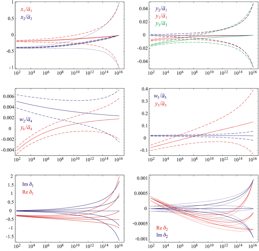
Figure 1: Upper four plots: RGE evolution of the MFV parameters for the SPS-1a benchmark point. The solid curves always show the evolution with mSUGRA type of initial conditions. In the upper-left panel, the dashed (dotted) lines show the evolution when $x_{1(2)}(M_{\text{GUT}})=\pm M_{0}^{2}$. In all other cases, for each parameter, only three curves are shown – the upper and lower ones (always shown as dashed) correspond to different initial conditions for that single parameter. Lower two plots: the real and imaginary parts of the mass insertions $\delta_{1(2)}\equiv(\delta_{RL}^{U(D)})^{32}/V_{ts}=(\delta_{RL}^{U(D)})^{31}/V_{td}$. For these plots, the initial conditions are varied independently for $\mathbf{A}^{U}$ and $\mathbf{A}^{D}$, allowing for a CP-phase as $A_{0}=re^{i\phi}$ with $r=0\rightarrow 200$ GeV and $\phi$ between $\pm 180{{}^{\circ}}$. Dashed lines in the $\delta_{2}$ plot show the impact of the initial conditions for $\mathbf{A}^{U}$, while the sensitivity of $\delta_{1}$ to those for $\mathbf{A}^{D}$ is negligible. The behaviours of the other mass-insertions, Eqs. (25, 26, 28), can easily be obtained from those of the parameters shown in the upper four plots. In particular, note that $y_{2}\left(M_{Z}\right)\ll x_{1}\left(M_{Z}\right)$, both because of the $\tan\beta$ suppression, and because of RGE effects.

The most prominent feature emerging from the figures is that all the parameters ratios tend to converge to one point at the low scale, independently of the starting point at the high scale – i.e. they show a fixed-point kind of behaviour, as recently observed in Ref. [5]. We stress, however, that by separating the leading parameters (the $\tilde{a}_{i}$’s and the $x_{i}$’s) from the suppressed ones, we can better see the behaviour of the small flavour violations, governed by the $y_{i}$’s and the $w_{i}$’s. Our analysis shows that these also converge to fixed points.

	$M_{\text{GUT}}$	$M_{Z}$
$\tilde{a}_{1}/M_{3}^{2}$	$0.16(1+\Delta_{1})$	$0.86+0.019\Delta_{1}$
$\tilde{a}_{2}/M_{3}^{2}$	$0.16(1+\Delta_{2})$	$0.81+0.015\Delta_{2}$
$\tilde{a}_{3}/M_{3}^{2}$	$0.16(1+\Delta_{3})$	$0.80+0.019\Delta_{3}$
$\tilde{a}_{4}/(-y_{t}M_{3})$	$0.40(1+\Delta_{4})$	$0.81+0.03\Delta_{4}$
$\tilde{a}_{5}/(-y_{b}M_{3})$	$0.40(1+\Delta_{5})$	$1.48+0.14\Delta_{5}$
$x_{1}/\tilde{a}_{1}$	$\delta_{1}$	$-0.18-0.003\Delta_{2}-0.01\Delta_{4}+0.02\delta_{1}-0.003\delta_{2}$
$y_{1}/\tilde{a}_{1}$	$\epsilon_{1}t_{\beta}^{2}\lambda^{6}$	$(-7.6+0.1\Delta_{1}-0.1\Delta_{3}-1.1\Delta_{5}+0.3\epsilon_{1})\cdot 10^{-3}$
$y_{2}/\tilde{a}_{1}$	$\epsilon_{2}t_{\beta}^{2}\lambda^{6}$	$(4.4-0.1\Delta_{1}+1.1\Delta_{4}+1.4\Delta_{5}-0.4\delta_{1}-0.4\epsilon_{1}$
		$+3.0\epsilon_{2}-2.5\epsilon_{4}-4.8\delta_{5})\cdot 10^{-4}$
$x_{2}/\tilde{a}_{2}$	$\delta_{2}$	$-0.38-0.01\Delta_{1}-0.02\Delta_{4}-0.01\delta_{1}+0.02\delta_{2}$
$y_{3}/\tilde{a}_{3}$	$\epsilon_{3}t_{\beta}^{2}\lambda^{6}$	$(-1.53-0.02\Delta_{1}+0.01\Delta_{1}+0.02\Delta_{3}+0.03\Delta_{4}-0.2\Delta_{5}$
		$-0.02\delta_{1}+0.04\epsilon_{3}-0.2\delta_{5})\cdot 10^{-2}$
$w_{1}/\tilde{a}_{3}$	$0$	$\sim-10^{-6}$
$y_{4}/\tilde{a}_{4}$	$c_{t}/y_{t}+\epsilon_{4}t_{\beta}^{2}\lambda^{6}$	$(-4.1-0.1\Delta_{4}-0.6\Delta_{5}+2.3\epsilon_{4})\cdot 10^{-3}$
$w_{2}/\tilde{a}_{4}$	$y_{c}/y_{t}+\eta_{2}\lambda^{4}$	$(5.1-0.4\Delta_{4}+0.7\eta_{2})\cdot 10^{-3}$
$y_{5}/\tilde{a}_{5}$	$c_{b}/y_{b}+\delta_{5}$	$-0.079-0.012\Delta_{4}-0.003\Delta_{5}+0.084\delta_{5}$
$w_{3}/\tilde{a}_{5}$	$y_{s}/y_{b}+\eta_{3}\lambda^{2}$	$0.019-0.002\Delta_{5}+0.005\eta_{3}$
$w_{4}/\tilde{a}_{5}$	$\eta_{4}\lambda^{4}$	$(1.0+0.1\Delta_{4}-0.1\Delta_{5}+0.2\eta_{3}+2.3\eta_{4})\cdot 10^{-4}$

Table 1: Dependence of the MFV parameters on the initial conditions when these are taken in the neighbourhood of the SPS-1a benchmark point. Any correction below one percent has been omitted.

The analytical solutions discussed above allow us to clearly understand the origin of these fixed points. First of all, we stress that indeed the running of the $\tilde{a}_{i}$’s is almost independent from the $x_{i}$’s, (which come in only through the combination $S$), and is strongly dominated by the term proportional to the gluino mass and strong gauge coupling, cf. Eq. (47). Table 1 shows that the $\tilde{a}_{i}$’s tend to the value $8|M_{3}|^{2}/9$ (for $=1,2,3$) at the low scale, up to small corrections, which of course can be calculated exactly with Eq. (47). For $\tilde{a}_{4,5}$, we do not have an explicit analytical solution, but from Eq. (50) we see that the integral over the function $f$ tends to a value of the order $y_{t,b}M_{3}(t)$ at the low scale. For $\tilde{a}_{4}$ ($\tilde{a}_{5}$), the integral $G_{\tilde{a}_{4(5)}}$ decreases (increases) from $1$ to about $0.4$ ($3.3$) in going from the GUT to the electroweak scale, and so we understand why the proportionality factor is smaller (larger) than one at the electroweak scale.

The analytical solutions for the $x_{i}$’s, Eqs. (53, 54), also explain the corresponding numbers in Table 1 and Fig. 1. First of all, the values of $x_{1}$ and $x_{2}$ at the electroweak scale, with initial conditions $x_{1}(t_{0})=x_{2}(t_{0})=0$, satisfy the relation $2x_{1}(t)=x_{2}(t)$ according to the solutions (53, 54) – a comparison to the numerical solution of the exact RGE’s shows that this is indeed verified to better than one per mil. We can therefore consider the solution of only one of the two, which reads:

$$x_{1}(t)=\frac{m_{0}^{2}}{6}\left[G_{n_{1}}(t)-1\right]-\frac{G_{n_{1}}(t)}{3N}\!\!\int_{t}^{t_{0}}\!\!\!\!dt^{\prime}\frac{f_{n_{1}}(t^{\prime})-f_{n_{2}}(t^{\prime})}{G_{n_{1}}(t^{\prime})}+\frac{1}{3N}\!\!\int_{t}^{t_{0}}\!\!\!\!dt^{\prime}f_{n_{2}}(t^{\prime})\left[1-\frac{G_{n_{1}}(t)}{G_{n_{1}}(t^{\prime})}\right].$$ (58)

At the electroweak scale $t_{\text{ew}}$ the three terms contribute, respectively

$$x_{1}(t_{\text{ew}})=-(1.3+73.1+2.9)\cdot 10^{3}=-77.2\cdot 10^{3}\;\mathrm{GeV}^{2}\;,$$ (59)

which shows that the dominating contribution comes from the integral over $f_{n_{1}}-f_{n_{2}}$ which contains only the $\tilde{a}_{i}$’s. In the ratio $x_{1}/a_{1}$, this is the part which tends to a small constant value at the electroweak scale, which almost looks like a fixed point. To understand why this almost looks like a fixed point, we have to analyze the dependence of $x_{1}(t)$ on the initial conditions. The relevant formulae have been given above, cf. Eq. (55), and show a linear dependence, with coefficients of order one. If we set, e.g. $x_{1}(t_{0})=\tilde{a}_{1}(t_{0})\delta_{1}$ and $x_{2}(t_{0})=\tilde{a}_{2}(t_{0})\delta_{2}$, as indicated in Table 1, then at the electroweak scale the effect is equal to:

$$\frac{\Delta x_{1}}{\tilde{a}_{1}} =\delta_{1}\frac{\tilde{a}_{1}(t_{0})}{\tilde{a}_{1}(t_{\text{ew}})}\frac{G_{n_{1}}(t_{\text{ew}})+5}{6}+\delta_{2}\frac{\tilde{a}_{2}(t_{0})}{\tilde{a}_{1}(t_{\text{ew}})}\frac{G_{n_{1}}(t_{\text{ew}})-1}{6}\;,$$ (60)

$$\frac{\Delta x_{2}}{\tilde{a}_{2}} =\delta_{1}\frac{\tilde{a}_{1}(t_{0})}{\tilde{a}_{2}(t_{\text{ew}})}\frac{G_{n_{1}}(t_{\text{ew}})-1}{3}+\delta_{2}\frac{\tilde{a}_{2}(t_{0})}{\tilde{a}_{2}(t_{\text{ew}})}\frac{G_{n_{1}}(t_{\text{ew}})+2}{3}\;,$$

where $\Delta x_{i}\equiv x_{i}(t_{\text{ew}})_{|_{\delta_{k}\neq 0}}-x_{i}(t_{\text{ew}})_{|_{\delta_{k}=0}}$, and inserting the numbers $G_{n_{1}}(t_{\text{ew}})=0.228$, and $\tilde{a}_{1}(t_{0})/\tilde{a}_{1}(t_{\text{ew}})=0.023$, $\tilde{a}_{2}(t_{0})/\tilde{a}_{2}(t_{\text{ew}})=0.024$, valid for the initial conditions specified in Table 1, one perfectly reproduces the numbers there. Similarly one can explain why the sensitivity to the initial conditions of the $\tilde{a}_{i}$’s is small: these enter through the second integral in Eq. (58) and contribute as follows. If we take $\tilde{a}_{i}(t_{0})=m_{0}^{2}(1+\Delta_{i})$ for $i=1,2,3$ and $\tilde{a}_{4(5)}(t_{0})=y_{t(b)}(t_{0})A_{0}(1+\Delta_{4(5)})$ then we have (for $\Delta x_{1}\equiv x_{i}(t_{\text{ew}})_{|_{\Delta_{k}\neq 0}}-x_{i}(t_{\text{ew}})_{|_{\Delta_{k}=0}}$)

$$\Delta x_{1} \!\!=\!\!-m_{0}^{2}(\Delta_{1}+\Delta_{2})\frac{G_{n_{1}}(t_{\text{ew}})}{3N}\int_{t_{\text{ew}}}^{t_{0}}dt^{\prime}\frac{6y_{t}^{2}(t^{\prime})}{G_{n_{1}}(t^{\prime})}-y_{t}(t_{0})A_{0}\Delta_{4}\frac{G_{n_{1}}(t_{\text{ew}})}{3N}\int_{t_{\text{ew}}}^{t_{0}}dt^{\prime}\frac{12\tilde{a}_{4}(t^{\prime})G_{a_{4}}(t^{\prime})}{G_{n_{1}}(t^{\prime})}$$

$$\!\!=\!\!-m_{0}^{2}\left[0.13(\Delta_{1}+\Delta_{2})+0.38\Delta_{4}\right]\;.$$ (61)

Dividing these numbers by $\tilde{a}_{1}(t_{\text{ew}})$ one reproduces the numbers in Table 1. Note that the sensitivity of $x_{1}/\tilde{a}_{1}$ to $\Delta_{1}$ receives another contribution due to the denominator dependence on $\Delta_{1}$. This is easy to calculate and brings the total coefficient below $1\%$ – for this reason a term with $\Delta_{1}$ does not appear in the line for $x_{1}/\tilde{a}_{1}$. We stress again that while the sensitivity of $x_{1}$ itself to the initial conditions of the parameters which appear in its beta function is described by a coefficient smaller than one, but not tiny, the ratio $x_{1}/\tilde{a}_{1}$ has tiny coefficients because $\tilde{a}_{1}(t_{0})/\tilde{a}_{1}(t_{\text{ew}})$ is tiny for the initial conditions given by the SPS-1a benchmark point.

All other coefficients appearing in Table 1, which specify the sensitivity of the various parameters to the initial conditions of all the others, can be understood analogously on the basis of our approximate analytical formulae.

Finally, concerning the CP-violating phases, we see from Fig. 1 that if $\delta_{LR}^{U}$ or $\delta_{LR}^{D}$ have an imaginary part at the GUT scale, even if large, it is much suppressed by the RGE effects. This is easily understood on the basis of the simplified analytical solutions: the imaginary part of $\tilde{a}_{4}$ misses the piece of the beta function which is responsible for the fast running of the real part, cf. (48). At the electroweak scale, only a residual phase remains, which acts as a small correction to the CKM one present in $V_{ts}$ or $V_{td}$. Note that at moderate $\tan\beta$, $\delta_{LR}^{D}$ is significantly affected by the initial conditions for $\delta_{LR}^{U}$: a phase for the latter can generate one for the former. On the other hand, any phase present in the trilinear terms has only a very limited effect on $y_{2}$, relevant for $(\delta_{LL})_{32}$ and $(\delta_{LL})_{31}$ mass-insertions. This follows also from Table 1, where it is apparent that the initial conditions for the trilinear terms affect only mildly the final value of $y_{2}$ at the electroweak scale. Conversely, if $y_{2}\left(t_{0}\right)$ has a large imaginary part, its running is very similar to the real part, i.e., it also decreases dramatically (see upper right plot in Fig. 1). Further, looking at the RGE’s, $y_{2}$ cannot communicate its phase to the trilinear terms. Therefore, all in all, if the SPS-1a is extended to include as many CP-violating phases as allowed by MFV at the GUT scale, all these phases are strongly suppressed at the electroweak scale. In that case, MFV essentially collapses onto the real parameter case, usually considered in the literature (see e.g. [12]), where all CP-violating observables are tuned entirely by the CKM phase.

4.3 Running from the electroweak up to the GUT scale

The numerical analysis of the SPS-1a benchmark point has shown that if one assumes that the MFV hypothesis is valid at the GUT scale, one has rather definite predictions at the low scale. We can now turn the question around and ask how MFV evolves towards the high scale if one assumes to know the parameters at the low scale. In particular, it is interesting to analyze what happens if the boundary conditions at the low scale are chosen such that they are rather far from the “fixed point” discussed above, but still well within the naturalness assumption of MFV.

We illustrate this in Fig. 2, in which we use as boundary condition at $\mu=M_{Z}$ all the values obtained from the evolution of the SPS-1a point, with the exception of $x_{1,2}$ for which we use $x_{1,2}(M_{Z})=-x_{1,2}^{\text{SPS-1a}}(M_{Z})$.

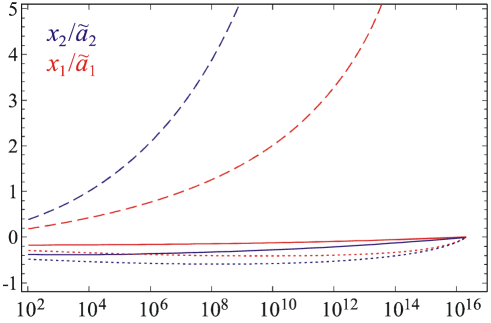
Figure 2: RGE evolution of the MFV parameters for the SPS-1a benchmark point, if the boundary conditions are fixed at the low scale. The dashed (dot-dashed) lines correspond to the change of boundary conditions $x_{1(2)}(M_{Z})=-x_{1(2)}^{\text{SPS-1a}}(M_{Z})$. The curves quitting the plot reach $x_{1}/\tilde{a}_{1}\approx 18$ and $x_{2}/\tilde{a}_{2}\approx 40$ at the GUT scale.

The figure shows that a point far from the “fixed point” at the low scale evolves to very high values of the MFV parameters at the high scale. This behaviour is easily understood on the basis of our analytical solution: from Table 1 we read off that a change of natural size of the initial conditions for $x_{1}$ produces a change of about $15\%$ at the low scale. So, if we want to induce a change of $200\%$ at the low scale, we need to make a change of more than one order of magnitude at the high scale. One could imagine changing more parameters at the same time in such a way that the evolution would be of MFV type all the way to the GUT scale. Table 1 shows, however, that this is not possible. Changing any of the other parameter around the SPS-1a benchmark points, while staying in a range compatible with MFV, does never generate a large change for $x_{1}/\tilde{a}_{1}$ at the low scale (similar conclusions can be reached for most other parameters).

The analysis of the previous section points to a possible way out: if the ratio $\tilde{a}_{1}(t_{0})/\tilde{a}_{1}(t_{\text{ew}})$ were of order one instead of $10^{-2}$, much larger changes in the low energy MFV parameters would become possible. This ratio, however, is completely fixed by the RGE’s and initial conditions, cf. Eq. (47) and can be changed significantly only by changing $\tilde{a}_{1}(t_{0})$ with respect to $M_{3}(t_{0})$ such that the former becomes at least as large as the term proportional to the gluino mass squared in Eq. (47). This, however, brings us far away from the SPS-1a point, and moreover, will tend to make the squarks heavier, which makes their contribution to low-energy flavour violations, and correspondingly the phenomenological interest, smaller. Such a situation is similar to the one realized in the case of the SPS-4 points (independently of the size of $\tan\beta$), as we will discuss in the next section.

We conclude that, if the spectrum at the low scale corresponds to the SPS-1a input at the high scale (note that the RGE’s discussed here show that an MFV-compatible change of the boundary conditions at the high scale has barely any influence on the spectrum), and if the values of the MFV parameters measured at the low scale are far away from those given in Table 1, then the MFV hypothesis has to break down somewhere before reaching the GUT scale.

This may indicate that either MFV has emerged from the RGE evolution of the parameters, starting from a non MFV kind of MSSM, or that the MFV parameters have a dynamical origin at a scale much lower than the GUT scale. The former solution cannot be really investigated with our simplified RGE’s, because if any of the MFV parameters is far from its assumed order, our RGE’s lose their accuracy. One would have to study this solution with the full RGE’s, and see how much fine-tuned it is, or whether it can viewed as natural in any sense. We leave this question open.

5 Running MFV in the large $\tan\beta$ case

5.1 Analytical solutions

When $\tan\beta\sim 1/\lambda^{3}$, the parameters $y_{i}$ become in principle of order one and cannot be neglected. The system of the RGE’s is then not amenable anymore to an analytical solution. The differential equations are all coupled and a diagonalization, although possible in principle, is too complicated to be of any use. Therefore, we start directly with the numerical analysis and make some remarks about how one can understand Table 2 on the basis of the analytical solutions provided in the previous section, plus some corrections specific to the large $\tan\beta$ case.

5.2 Numerical example: the SPS-4 benchmark point

The SPS-4 benchmark point has $m_{0}=400$ GeV, $m_{1/2}=300$ GeV, $A_{0}=0$ at the GUT scale, and $\tan\beta=50$. With these parameters, too large supersymmetric contributions to $b\rightarrow s\gamma$ are generated, such that the total rate comes out much lower than the measured one – this point is therefore not compatible with the phenomenology at the low scale. We use it nonetheless for illustration purposes. Another important aspect is that $A_{0}$ is set to zero at the GUT scale, and so $\tilde{a}_{4}=\tilde{a}_{5}=0$ there. If we want to vary the flavour violating parameters in the trilinear couplings, we first need to define a scale of naturalness for them. For this we use the value of $\tilde{a}_{4}$ and $\tilde{a}_{5}$ at the low scale and set at $\mu=M_{\mathrm{GUT}}$

$$y_{4}\sim-y_{t}M_{3}t_{\beta}^{2}\lambda^{6}\;,\;\;\;\;w_{2}\sim-y_{t}M_{3}\lambda^{4}\;\;,$$ (62)

and

$$y_{5}\sim-y_{b}M_{3}\;,\;\;\;\;w_{3}\sim-y_{b}M_{3}\lambda^{2}\;,\;\;\;\;w_{4}\sim-y_{b}M_{3}\lambda^{4}\;\;.$$ (63)

As soon as we make any of these parameters different from zero, their ratio to $\tilde{a}_{4}$ or $\tilde{a}_{5}$ at the high scale therefore diverges, as it is seen in Fig. 3. Running down to the low scale, however, the ratio quickly converges to its natural range, and becomes one or smaller.

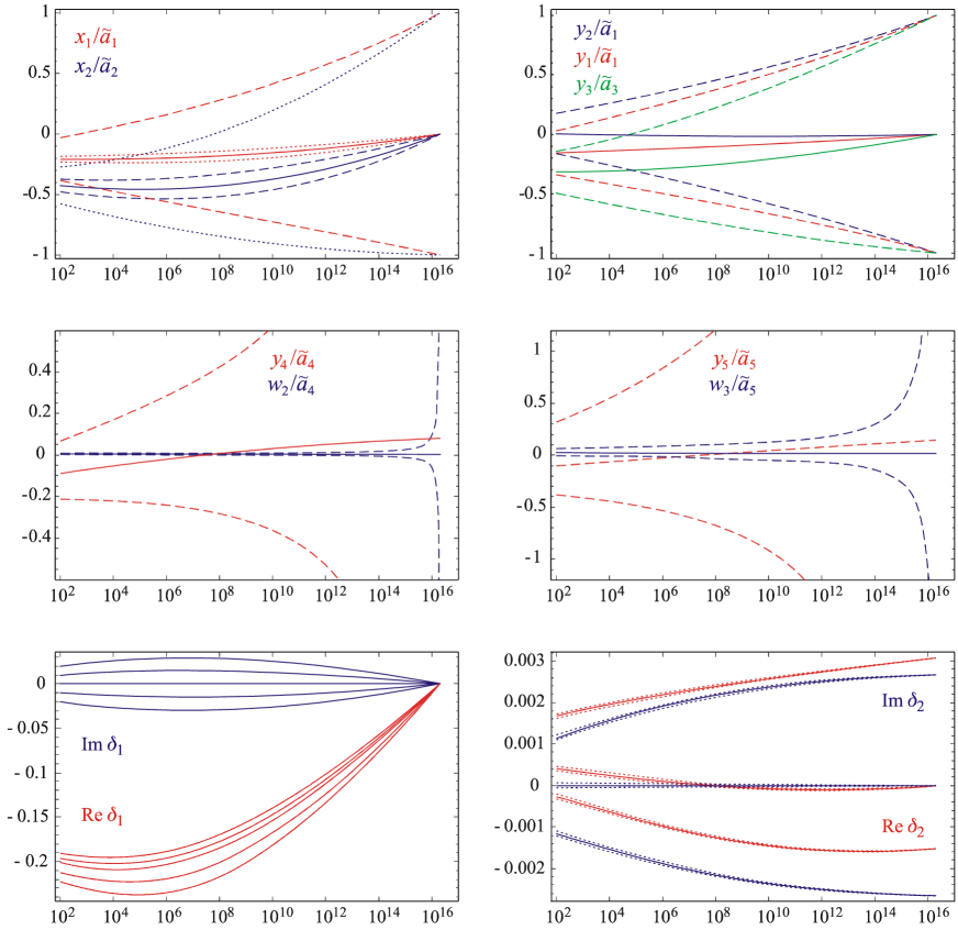
Figure 3: Upper four plots: RGE evolution of the MFV parameters for the SPS-4 benchmark point. The solid curves always show the evolution of the mSUGRA type of initial conditions. In the upper-left panel the dashed (dotted) lines show the evolution when $x_{1(2)}(M_{\text{GUT}})=\pm M_{0}^{2}$. In all other cases, for each parameter only three curves are shown – the upper and lower ones (always shown as dashed) correspond to different initial conditions for that single parameter. Lower two plots: the mass-insertions $\delta_{1(2)}\equiv(\delta_{RL}^{U(D)})^{32}/V_{ts}=(\delta_{RL}^{U(D)})^{31}/V_{td}$, with the initial conditions at the GUT scales varied as explained in the text, but allowing in addition for a large CP-phase (between $\pm 180{{}^{\circ}}$). In this case, $\delta_{1}\sim\tilde{a}_{4}$ is entirely radiatively generated, since $\tilde{a}_{4}=0$ is set to zero at the GUT scale. The behaviours of the other mass-insertions, Eqs. (25, 26, 28), can easily be obtained from those of the parameters shown in the upper four plots. In particular, note that though $y_{2}\left(M_{Z}\right)$ is still smaller than $x_{1}\left(M_{Z}\right)$, it is much less suppressed by RGE effects than in the SPS-1a case, and so is its CP-violating phase.

The fact that $\tan\beta$ is so large means that most of the $y_{i}$ and $w_{i}$ parameters change their order, since $\lambda^{3}\tan\beta\sim 0.6$. The curves in Figure 3 show that the behaviour is indeed different than for the SPS-1a benchmark point. Since now more parameters are of order one (or almost), the mutual influences of the various parameters are more important, though still quite small, as can be seen in Table 2. The most prominent difference, however, is that the “fixed points” are now much weaker – the value of the parameters at the low scale is influenced more sensitively by the starting values at the high scale. The same two statements can be made for the imaginary parts of the complex coefficients: their suppression through RGE effects is now much weaker, and the presence of a CP-phase for one parameter is felt more strongly by the others. For example, if $\mathbf{A}^{U}$ and/or $\mathbf{A}^{D}$ involve complex phases at the GUT scale, $y_{2}$ does develop a small but significant phase at the low scale.

	$M_{\text{GUT}}$	$M_{Z}$
$\tilde{a}_{1}/M_{3}^{2}$	$1.8(1+\Delta_{1})$	$1.06+0.21\Delta_{1}+0.01\Delta_{2}+0.006\Delta_{3}$
$\tilde{a}_{2}/M_{3}^{2}$	$1.8(1+\Delta_{2})$	$1.01+0.02\Delta_{1}+0.17\Delta_{2}+0.02\Delta_{3}+0.008(\delta_{1}-2\delta_{2})$
$\tilde{a}_{3}/M_{3}^{2}$	$1.8(1+\Delta_{3})$	$1.00-0.01\Delta_{1}+0.02\Delta_{2}+0.21\Delta_{3}-0.004(\delta_{1}-2\delta_{2})$
$\tilde{a}_{4}/(-y_{t}M_{3})$	$\Delta_{4}$	$0.78+0.09\Delta_{4}+0.02\Delta_{5}-0.09\epsilon_{4}-0.03\delta_{5}$
$\tilde{a}_{5}/(-y_{b}M_{3})$	$\Delta_{5}$	$0.93+0.02\Delta_{4}+0.16\Delta_{5}-0.03\epsilon_{4}-0.17\delta_{5}$
$x_{1}/\tilde{a}_{1}$	$\delta_{1}$	$-0.21+0.01\Delta_{1}-0.02\Delta_{2}-0.02\Delta_{4}+0.18\delta_{1}$
		$-0.02\delta_{2}+0.01\epsilon_{1}+0.02\epsilon_{4}-0.01\delta_{5}$
$y_{1}/\tilde{a}_{1}$	$\epsilon_{1}t_{\beta}^{2}\lambda^{6}$	$-0.16+0.01\Delta_{1}-0.02\Delta_{3}-0.03\Delta_{5}+0.01\delta_{1}$
		$+0.07\epsilon_{1}-0.01\epsilon_{3}+0.02\delta_{5}$
$y_{2}/\tilde{a}_{1}$	$\epsilon_{2}t_{\beta}^{2}\lambda^{6}$	$(0.6-0.1\Delta_{1}+0.6\Delta_{4}+0.7\Delta_{5}-1.4\delta_{1}-0.9\epsilon_{1}$
		$+6.3\epsilon_{2}-0.9\epsilon_{4}-1.6\delta_{5})\cdot 10^{-2}$
$x_{2}/\tilde{a}_{2}$	$\delta_{2}$	$-0.43-0.04\Delta_{1}+0.01\Delta_{2}+0.01\Delta_{3}-0.03\Delta_{4}+0.01\Delta_{5}$
		$-0.05\delta_{1}+0.15\delta_{2}-0.02\epsilon_{1}-0.04\epsilon_{2}-0.01\epsilon_{4}+0.01\delta_{5}$
$y_{3}/\tilde{a}_{3}$	$\epsilon_{3}t_{\beta}^{2}\lambda^{6}$	$-0.32-0.046\Delta_{1}+0.012\Delta_{2}+0.02\Delta_{3}+0.01\Delta_{4}-0.04\Delta_{5}$
		$-0.04\delta_{1}+0.01\delta_{2}-0.02\epsilon_{1}-0.03\epsilon_{2}+0.06\epsilon_{3}-0.04\delta_{5}$
$w_{1}/\tilde{a}_{3}$	$0$	$\sim 10^{-5}$
$y_{4}/\tilde{a}_{4}$	$\epsilon_{4}t_{\beta}^{2}\lambda^{6}$ $(^{\ast})$	$-0.09-0.02\Delta_{4}-0.04\Delta_{5}+0.14\epsilon_{4}+0.02\delta_{5}$
$w_{2}/\tilde{a}_{4}$	$\eta_{2}\lambda^{4}$	$(5.0-1.1\Delta_{4}-0.1\Delta_{5}+0.3\epsilon_{4}+1.9\eta_{2}+0.3\delta_{5})\cdot 10^{-3}$
$y_{5}/\tilde{a}_{5}$	$\delta_{5}$          $(^{\ast})$	$-0.10-0.046\Delta_{4}-0.023\Delta_{5}+0.015\epsilon_{4}+0.36\delta_{5}$
$w_{3}/\tilde{a}_{5}$	$\eta_{3}\lambda^{2}$	$0.023-0.005\Delta_{5}+0.001\epsilon_{4}+0.003\delta_{5}+0.026\eta_{3}$
$w_{4}/\tilde{a}_{5}$	$\eta_{4}\lambda^{4}$	$(1.2+0.3\Delta_{4}-0.2\Delta_{5}+0.1\epsilon_{4}+0.2\delta_{5}+1.3\eta_{3}+7.8\eta_{4})\cdot 10^{-4}$

Table 2: Dependence of the MFV parameters on the initial conditions for the SPS-4 point. Any correction below one percent has been omitted.
$(^{\ast})$ Since $\tilde{a}_{4(5)}(M_{\text{GUT}})=0$, at this scale we normalize $y_{4}$ and $w_{2}$ ($y_{5}$, $w_{3}$ and $w_{4}$) by $-y_{t}M_{3}$ ($-y_{b}M_{3}$).

Can we understand why this happens? Also, and more importantly, is it the large $\tan\beta$ or the large $m_{0}$ which is responsible for the different behaviour of the SPS-4 benchmark point? A first clue is given in Fig. 4, where the boundary conditions are set according to the SPS-1a, but for $\tan\beta=50$. Obviously, the fixed point behaviour is to a large extent unaffected by $\tan\beta$, even for the $y_{i}$, which are now of $\mathcal{O}(1)$. In particular, remark that $y_{2}$ still converge towards zero, and so does its phase.

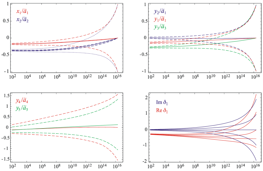
Figure 4: RGE evolution of the MFV parameters for the SPS-1a benchmark point, but with $\tan\beta=50$. As in Fig. 1, the initial conditions at the GUT scale are varied, but now allowing larger range for the $y_{i}$, which can be of $\mathcal{O}(1)$. Still, the quasi fixed-point behaviour is obviously largely independent of $\tan\beta$. The corresponding plot for $\delta_{2}$ is similarly close to the $\tan\beta=10$ one. Those for $w_{1,2}$ are not shown because these parameters stay very small, even with $\tan\beta=50$.

It is thus the larger $m_{0}$ which should be responsible for the different behaviour shown in Fig. 3. This is confirmed with the help of the analytical solutions, and Table 2. Consider for example $x_{1}(t_{\text{ew}})$, which now depends ten times more strongly than in the SPS-1a case on its initial condition $x_{1}(t_{0})$. If we ignore for a moment that the beta function of $x_{1}$ also receives a contribution from $y_{2}$ and $y_{5}$, which are potentially large, and evaluate the coefficient in front of $\delta_{1}$ in the seventh row of Table 2 with the help of Eq. (55) we get:

$$\frac{\Delta x_{1}(t_{\text{ew}})}{a_{1}(t_{\text{ew}})}=\delta_{1}\frac{a_{1}(t_{0})}{a_{1}(t_{\text{ew}})}\frac{G_{n_{1}}(t_{\text{ew}})+5}{6}=\delta_{1}\,0.21\cdot\frac{5.21}{6}=0.18\;,$$ (64)

in perfect agreement with the number in the table. The reason for the enhanced sensitivity to the initial conditions is due to the less strong growth of $\tilde{a}_{1}$ in going from the GUT to the electroweak scale – the extra dependence on the initial conditions of $x_{1}$ coming from the terms proportional to $y_{2}$ and $y_{5}^{2}$ is negligible, as we have explicitly checked (the reason can be understood rather easily: the $y_{i}$’s depend on $x_{1}$ through the beta function and vice-versa – so the extra dependence of $x_{1}(t_{\text{ew}})$ on its initial conditions at the GUT scale comes in through the beta function of the beta function and is therefore suppressed by two powers of $1/N$). In fact, even the value of $x_{1}(t_{\text{ew}})$ for initial conditions of the mSUGRA type can be understood rather well on the basis of the analytical formulae obtained in the case of moderate $\tan\beta$: the relation $2x_{1}(t)=x_{2}(t)$ holds to better than one percent and Eq. (58) yields numerically:

$$x_{1}(t_{\text{ew}})=-(2.10+13.76+0.42)\cdot 10^{4}=-16.28\cdot 10^{4}\;\mathrm{GeV}^{2}\;,$$ (65)

whereas the value obtained solving the exact RGE’s numerically is $-16.11\cdot 10^{4}$ GeV² – the approximate analytical solutions obtained in the moderate $\tan\beta$ case work here surprisingly well, to one percent accuracy.

6 Conclusions

In this paper, we have revisited the formulation of minimal flavour violation (MFV) within Minimal Supersymmetric extensions of the Standard Model (MSSM), and linked it to a counting rule which keeps track of the hierarchies in the Yukawa couplings and in the CKM matrix in a coherent way. This allowed us to move continuously and in a controlled manner, between the moderate and the large $\tan\beta$ case, keeping control over the expected order of magnitude of the different terms. We have argued that to implement these counting rules in an efficient way, it is convenient to express the soft SUSY breaking terms of the MSSM in a different basis than in the conventional MFV. In order to study the renormalization group equations of the MFV parameters, we have projected the beta functions of the soft SUSY breaking terms on this basis and checked that the beta functions obey the same counting rules as the coefficients themselves. We have then studied the behaviour of the running of the MFV parameters numerically, and first checked that this reproduces the full running with MFV boundary conditions at the level of accuracy at which we expected them to work.

In the moderate $\tan\beta$ case, we were able to provide approximate analytical solutions to the RGE’s of the MFV parameters, and we discussed, in the case of the SPS-1a benchmark point, the behaviour of the MFV parameters under the running. We confirmed the finding of Ref. [5] about a quasi fixed-point behaviour of these, and could explain it in detail with the help of our analytical solutions. The crucial observation is that the flavour blind part of the soft SUSY-breaking terms, the $a_{i}$ parameters, run fast, like the gluino masses, whereas all the terms with a nontrivial flavour structure (the $x_{i}$’s, in our basis) grow less rapidly – their beta functions do not contain the gaugino masses, but at best the $a_{i}$’s. This hierarchy in the beta functions explains why the ratios of the flavour-violating parameters to the flavour-blind ones tend to a small, finite value at the low scale. The only possibility we have identified to avoid this, and to make a larger range of values at the low scale at all possible, is to increase the value of the $a_{i}$’s at the GUT scale – this, however, makes the squark masses heavier, which in turn suppresses flavour violations at low energies.

Our analysis of the SPS-4 benchmark point, which has $\tan\beta=50$, shows that the picture does not change substantially for large $\tan\beta$. More parameters (the $y_{i}$’s in our notation) may become of order one, but their RGE’s are not particularly different from those of the $x_{i}$’s (they also contain at best the $a_{i}$’s in their beta functions, and do not grow as fast), nor do they influence the other parameters of order one in a substantial way.

The picture which emerges from this analysis is that, if MFV is valid and has its origin at the GUT scale (or at any other high scale much higher than the SUSY breaking one), then it is a much more constraining framework than if one assumes it to be valid just at the electroweak scale.

This is particularly true for the CP-violating phases. Throughout our study, we have allowed MFV coefficients to have imaginary parts, whenever allowed by the hermiticity of squark soft SUSY breaking mass terms. The first important observation is that MFV does allow for new CP-violating phases not only in the trilinear terms, but also in the LL sector. This latter phase could have significant impacts on the MFV predictions for $b\rightarrow s$ and $b\rightarrow d$ observables (but not for $s\rightarrow d$ ones, where it is absent). However, if MFV has its origin at the GUT scale, and $\tan\beta$ is not too large, we have shown that all the CP-violating phases are strongly suppressed at the low-scale. This behaviour is essentially unaltered when $\tan\beta$ is large, though in that case, the initial conditions at the GUT scale have to be modified. In particular, when squark soft SUSY breaking mass terms are as large as in the SPS-4 benchmark point, the suppression is much less pronounced.

A final comment about leptons, which in this analysis have only played a marginal role. One can of course apply similar ideas in that sector also, as has been shown by Ref. [22]. Moreover, if one considers a grand unified theory, one has a more constrained framework, and has relations between the MFV parameters in the lepton and in the quark sector [23] (indeed, independently from any MFV hypothesis, the relations between the two sectors have interesting phenomenological implications, [14]). While these connections are very interesting and worth investigating, they mostly concern the boundary conditions at the GUT scale – the RGE below the GUT scale are the standard MSSM ones. As a first analysis of the running of the MFV parameters, we therefore found it more convenient to concentrate ourselves only on the quark sector.

Appendix A Solving the RGE’s and boundary conditions

For our purpose, only the one-loop RGE’s are needed. At that order, the gauge, Yukawa, soft-breaking and Higgs sectors essentially decouple, and solving the RGE’s proceeds in steps. First, the RGE’s for the gauge couplings are solved,

$$\frac{d\alpha_{i}\left(t\right)}{dt}=\frac{1}{2\pi}\beta_{i}\alpha_{i}^{2}\;\;,\;\;\;\beta_{i}=\left(33/5,\,1,\,-3\right)\;.$$ (66)

Using, the $\overline{MS}$ values for simplicity, i.e. $\alpha_{em}^{-1}\left(M_{Z}\right)=127.904(17)$, $\sin^{2}\theta_{W}\left(M_{Z}\right)=0.23122(15)$, and $\alpha_{s}\left(M_{Z}\right)=0.1176(20)$, the unification scale and the corresponding value of the gauge coupling are found as

$$M_{G}=2.0\times 10^{16}\;\text{GeV},\ \ \alpha_{G}^{-1}(M_{G})=24.3\;,$$ (67)

if the MSSM running starts at the $M_{Z}$ scale, which we also assume for simplicity. The gaugino masses are required to unify at the same scale $M_{G}$ as the couplings,

$$M_{1}\left(M_{G}\right)=M_{2}\left(M_{G}\right)=M_{3}\left(M_{G}\right)\equiv m_{1/2}\;.$$ (68)

Their RGE’s are also solved to one-loop.

Second, the Yukawa couplings at the electroweak scale are set from the known fermion masses at that scale (again, we neglect the difference between $\overline{DR}$ and $\overline{MS}$ values for simplicity)

$$\begin{array}[c]{ccc}m_{u}\left(M_{Z}\right)=1.27\;\mathrm{MeV}\;,&m_{c}\left(M_{Z}\right)=0.619\;\mathrm{GeV}\;,&m_{t}\left(M_{Z}\right)=171.7\;\mathrm{GeV}\;,\\ m_{d}\left(M_{Z}\right)=2.9\;\mathrm{MeV}\;,&m_{s}\left(M_{Z}\right)=0.055\;\mathrm{GeV}\;,&m_{b}\left(M_{Z}\right)=2.89\;\mathrm{GeV}\;,\\ m_{e}\left(M_{Z}\right)=0.4866\;\mathrm{MeV}\;,&m_{\mu}\left(M_{Z}\right)=0.1027\;\mathrm{GeV}\;,&m_{\tau}\left(M_{Z}\right)=1.7462\;\mathrm{GeV}\;.\end{array}$$ (69)

as well as by setting $\tan\beta\equiv v_{u}/v_{d}$ and $v_{u}^{2}+v_{d}^{2}\simeq(174$ $\mathrm{GeV})^{2}$. Their one-loop RGE’s can then immediately be solved numerically. Running up according to either the full one-loop MSSM beta functions, or with the approximate MFV RGE’s, we find for $\tan\beta=10$:

$$|\mathbf{Y}_{u}^{\text{MFV}}\left(M_{G}\right)| =\left(\begin{array}[c]{ccc}0&0&0\\ 0.00032&0.0014&6.0\cdot 10^{-5}\\ 0.00459&0.0236&0.577\end{array}\right),\;\;\Delta\mathbf{Y}_{u}\lesssim\left(\begin{array}[c]{ccc}10^{-6}&10^{-6}&10^{-8}\\ 10^{-8}&10^{-7}&10^{-7}\\ 10^{-6}&10^{-6}&10^{-4}\end{array}\right)\;,$$ (76)

$$|\mathbf{Y}_{d}^{\text{MFV}}\left(M_{G}\right)| =\left(\begin{array}[c]{ccc}0&0&0\\ 0&0.000911&0\\ 5.03\cdot 10^{-5}&0.000259&0.0545\end{array}\right),\;\;\Delta\mathbf{Y}_{d}\lesssim\left(\begin{array}[c]{ccc}10^{-4}&10^{-9}&10^{-7}\\ 10^{-8}&10^{-7}&10^{-6}\\ 10^{-8}&10^{-7}&10^{-6}\end{array}\right)\;,$$ (83)

$$\mathbf{Y}_{e}^{\text{MFV}}\left(M_{G}\right) =\mathrm{diag}\left(0,\;0.0040,\;0.0675\right),\;\;\Delta\mathbf{Y}_{e}\lesssim\mathrm{diag}\left(10^{-5},\;10^{-8},\;10^{-7}\right)\;,$$ (84)

where $\Delta\mathbf{Y}=|\mathbf{Y}_{u}^{\text{MFV}}\left(M_{G}\right)|-|\mathbf{Y}_{u}^{\text{Full}}\left(M_{G}\right)|$, and for $\tan\beta=50$ (neglecting non-holomorphic corrections):

$$|\mathbf{Y}_{u}^{\text{MFV}}\left(M_{G}\right)|=\left(\begin{array}[c]{ccc}0&0&0\\ 0.00034&0.00146&6.2\cdot 10^{-5}\\ 0.0050&0.0259&0.683\end{array}\right),\;\;\Delta\mathbf{Y}_{u}\lesssim\left(\begin{array}[c]{ccc}10^{-6}&10^{-6}&10^{-8}\\ 10^{-6}&10^{-6}&10^{-5}\\ 10^{-4}&10^{-4}&10^{-2}\end{array}\right)\;,$$ (91)

$$|\mathbf{Y}_{d}^{\text{MFV}}\left(M_{G}\right)|=\left(\begin{array}[c]{ccc}0&0&0\\ 0&0.00613&0\\ 0.00047&0.00242&0.472\end{array}\right),\;\;\Delta\mathbf{Y}_{d}\lesssim\left(\begin{array}[c]{ccc}10^{-4}&10^{-8}&10^{-7}\\ 10^{-7}&10^{-5}&10^{-5}\\ 10^{-5}&10^{-5}&10^{-3}\end{array}\right)\;,$$ (98)

$$\mathbf{Y}_{e}^{\text{MFV}}\left(M_{G}\right)=\mathrm{diag}\left(0,\;0.0266,\;0.542\right),\;\;\Delta\mathbf{Y}_{e}\lesssim\mathrm{diag}\left(10^{-4},\;10^{-4},\;10^{-3}\right)\;.$$ (99)

This shows that our counting is valid at all scales. It also shows in practice how it is enforced: entries of absolute size at or below the $\mathcal{O}(10^{-4})$ are neglected (for consistency, since $m_{u}$, $m_{d}$ and $m_{e}$ are set to zero), while the non zero entries are reproduced up to $\mathcal{O}(10^{-2})$ corrections. This structure is shared by the squark and slepton soft-breaking terms, following Eq. (21). The evolution of the parameters used to describe the running of the full Yukawa couplings is shown in Fig. 5. The scalings of these parameters, in powers of $\lambda$, can be immediately read off these plots. We stress, however, that higher order terms in the RGE, as well as in the matching at the electroweak scale, are relevant for the precise values of the Yukawa couplings at the GUT scale. In particular, at the one-loop level, the Yukawa couplings fail to unify at the GUT scale, as shown in Fig. 5. This is of no concern for the present work. Rather, our purpose was to check whether the beta functions expanded according to our counting rules do indeed reproduce very precisely the full one loop RGE. As shown in Eqs. (84, 99), this is indeed the case, and there is a priori nothing preventing one to extend the present analysis to include higher order effects.

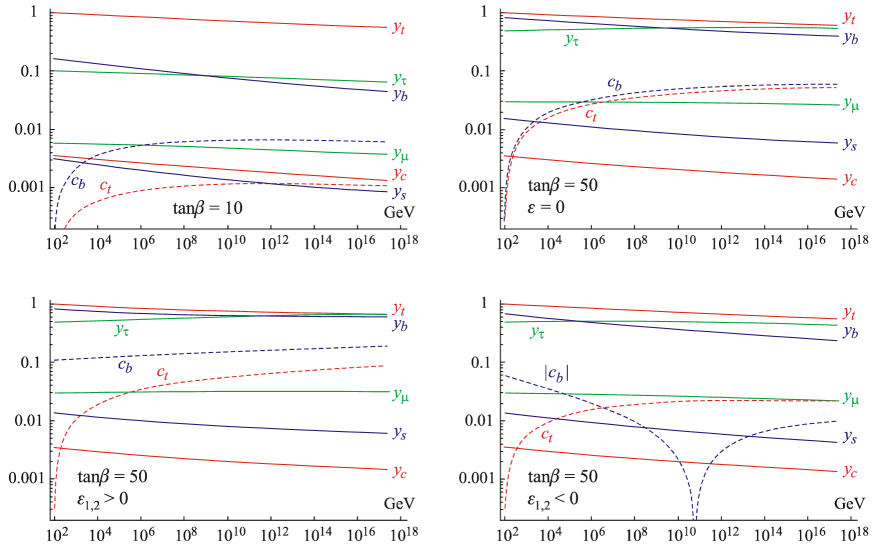
Figure 5: Up: RGE evolution of the Yukawa couplings, in terms of their skeleton structures given in Eq.(33), for $\tan\beta=10$ and $50$. The running obtained by solving the RGE of Eq.(35) or the full running projected back on Eq.(33) are indistinguishable. Down: the running of the parameters with large $\tan\beta$ initial conditions, as specified in Eq. (100). In the right plot, starting with $c_{b}\left(M_{Z}\right)<0$, the RGE drives it positive, hence the zero at about $10^{11}$ GeV.

In particular, to show the impact of the non-holomorphic corrections, we consider the simulated scenario corresponding to

$$\mathbf{\Delta}=\tan\beta\left(\varepsilon_{1}\mathbf{Y}_{u}^{\dagger}\mathbf{Y}_{u}+\varepsilon_{2}\mathbf{Y}_{d}^{\dagger}\mathbf{Y}_{d}\right)\;,$$ (100)

with $\tan\beta=50$ and $\varepsilon_{1}=\pm 0.002$, $\varepsilon_{2}=\pm 0.003$, which is in the ballpark of the values given e.g. in Ref. [21], but still small enough that $\eta_{i}\approx 1$ in Eq. (41). Such a correction can be accounted for by shifting the initial conditions for $y_{s}\left(M_{Z}\right)$, $y_{b}\left(M_{Z}\right)$ and $c_{b}\left(M_{Z}\right)$. Solving Eq. (38) iteratively, we find

$$\varepsilon_{1} =+0.002,\varepsilon_{2}=+0.003\Rightarrow y_{s}\left(M_{Z}\right)=0.0138,\;y_{b}\left(M_{Z}\right)=0.832,\;c_{b}\left(M_{Z}\right)=0.110\;,$$ (101)

$$\varepsilon_{1} =-0.002,\varepsilon_{2}=-0.003\Rightarrow y_{s}\left(M_{Z}\right)=0.0138,\;y_{b}\left(M_{Z}\right)=0.683,\;c_{b}\left(M_{Z}\right)=0.0595\;.$$ (102)

Taking these initial conditions, and running the Yukawa couplings according to Eq. (35), or using the full MSSM running, is numerically equivalent to within one part in $10^{-4}$, as in Eqs. (84, 99). The behavior of the parameters is shown in Fig. 5. As one can see, the parameter $c_{b}\left(\mu\right)$, though now slightly larger, is still sufficiently small to be counted as of order $\mathcal{O}(y_{b}\lambda^{2})$.

The third step is to solve the RGE’s for $m_{Hu}^{2}$, $m_{Hd}^{2}$, $\mathbf{m}_{Q}^{2}$, $\mathbf{m}_{U}^{2}$, $\mathbf{m}_{D}^{2}$, $\mathbf{A}^{U}$, $\mathbf{A}^{D}$, $\mathbf{m}_{L}^{2}$, $\mathbf{m}_{E}^{2}$, and $\mathbf{A}^{E}$, setting initial conditions at the high scale (details of which are given in the text). Typically, we start with

$$m_{Hu}^{2}\left(M_{G}\right)=m_{Hd}^{2}\left(M_{G}\right)\equiv m_{0}^{2}\;,$$

with $m_{0}\approx A_{0}$ also setting the scale of the squark and slepton soft-breaking terms.

The final step is to enforce the matching at the electroweak scale for the Higgs sector. The Higgs vacuum expectation values $v_{u}$ and $v_{d}$ are fixed from $\tan\beta$ and $M_{Z}$. Enforcing the correct Higgs potential, and knowing $m_{Hu}^{2}\left(M_{Z}\right)$ and $m_{Hd}^{2}\left(M_{Z}\right)$, gives $|\mu\left(M_{Z}\right)|$ and $b\left(M_{Z}\right)$, which can then be run up to the $M_{G}$ scale. Lowest order approximations are notoriously inadequate at this step, but this is of no concern for us since this matching and running is fully decoupled from the rest, in particular from the squark and slepton sector on which we concentrate.

Appendix B Relation between the $x_{i}$ and the $b_{i}$ parameters

The standard MFV basis of Ref. [2], and the one with the $X_{i}$ matrices adopted here are related to each other by a linear transformation. The MFV representation of the soft SUSY breaking terms given in Eq. (21), corresponds to the following in the standard basis (assuming real MFV coefficients for simplicity):

$$\mathbf{m}_{Q}^{2} =m_{0}^{2}\left[a_{1}+b_{1}\mathbf{Y}_{u}^{\dagger}\mathbf{Y}_{u}+b_{2}\mathbf{Y}_{d}^{\dagger}\mathbf{Y}_{d}+c_{1}(\mathbf{Y}_{d}^{\dagger}\mathbf{Y}_{d}\mathbf{Y}_{u}^{\dagger}\mathbf{Y}_{u}+\mathbf{Y}_{u}^{\dagger}\mathbf{Y}_{u}\mathbf{Y}_{d}^{\dagger}\mathbf{Y}_{d})\right]\;,$$

$$\mathbf{m}_{U}^{2} =m_{0}^{2}\left[a_{2}+b_{3}\mathbf{Y}_{u}\mathbf{Y}_{u}^{\dagger}\right]\;,$$

$$\mathbf{m}_{D}^{2} =m_{0}^{2}\left[a_{3}+\mathbf{Y}_{d}\left(b_{6}+b_{7}\mathbf{Y}_{u}^{\dagger}\mathbf{Y}_{u}\right)\mathbf{Y}_{d}^{\dagger}\right]\;,$$

$$\mathbf{A}^{U} =A_{0}\mathbf{Y}_{u}\,\left[a_{4}+b_{9}\mathbf{Y}_{u}^{\dagger}\mathbf{Y}_{u}+b_{10}\mathbf{Y}_{d}^{\dagger}\mathbf{Y}_{d}\right]\;,$$

$$\mathbf{A}^{D} =A_{0}\mathbf{Y}_{d}\,\left[a_{5}+b_{11}\mathbf{Y}_{u}^{\dagger}\mathbf{Y}_{u}+b_{12}\mathbf{Y}_{d}^{\dagger}\mathbf{Y}_{d}+c_{6}\mathbf{Y}_{d}^{\dagger}\mathbf{Y}_{d}\mathbf{Y}_{u}^{\dagger}\mathbf{Y}_{u}\right]\;.$$ (103)

The connection between both bases is explicitly given here:

$$\left(\begin{array}[c]{c}\tilde{a}_{1}\\ x_{1}\\ y_{1}\\ y_{2}\end{array}\right) =m_{0}^{2}\left(\begin{array}[c]{cccc}1&0&0&0\\ 0&y_{t}^{2}&c_{b}^{2}&2c_{b}y_{t}\bar{y}_{b}\bar{y}_{t}\\ 0&c_{t}^{2}&y_{b}^{2}&2c_{t}y_{b}\bar{y}_{b}\bar{y}_{t}\\ 0&c_{t}y_{t}&c_{b}y_{b}&2\left(c_{t}c_{b}+y_{b}y_{t}\right)\bar{y}_{b}\bar{y}_{t}\end{array}\right)\left(\begin{array}[c]{c}a_{1}\\ b_{1}\\ b_{2}\\ c_{1}\end{array}\right)\;,$$ (116)

$$\left(\begin{array}[c]{c}\tilde{a}_{2}\\ x_{2}\end{array}\right) =m_{0}^{2}\left(\begin{array}[c]{cc}1&0\\ 0&\bar{y}_{t}^{2}\end{array}\right)\left(\begin{array}[c]{c}a_{2}\\ b_{3}\end{array}\right)\;,$$ (123)

$$\left(\begin{array}[c]{c}\tilde{a}_{3}\\ y_{3}\\ w_{1}\end{array}\right) =m_{0}^{2}\left(\begin{array}[c]{ccc}1&0&0\\ 0&\bar{y}_{b}^{2}&\bar{y}_{t}^{2}\bar{y}_{b}^{2}\\ 0&-A\lambda^{2}c_{b}y_{s}&-A\lambda^{2}y_{s}y_{t}\bar{y}_{b}\bar{y}_{t}\end{array}\right)\left(\begin{array}[c]{c}a_{1}\\ b_{6}\\ b_{7}\end{array}\right)\;,$$ (133)

$$\left(\begin{array}[c]{c}\tilde{a}_{4}\\ y_{4}\\ w_{2}\end{array}\right) =A_{0}\left(\begin{array}[c]{ccc}y_{t}&y_{t}\bar{y}_{t}^{2}&c_{b}\bar{y}_{b}\bar{y}_{t}\\ c_{t}&c_{t}\bar{y}_{t}^{2}&y_{b}\bar{y}_{b}\bar{y}_{t}\\ y_{c}&0&0\end{array}\right)\left(\begin{array}[c]{c}a_{4}\\ b_{9}\\ b_{10}\end{array}\right)\;,$$ (143)

$$\left(\begin{array}[c]{c}\tilde{a}_{5}\\ y_{5}\\ w_{3}\\ w_{4}\end{array}\right) =A_{0}\left(\begin{array}[c]{cccc}y_{b}&c_{t}\bar{y}_{t}\bar{y}_{b}&y_{b}\bar{y}_{b}^{2}&c_{t}\bar{y}_{t}\bar{y}_{b}^{3}\\ c_{b}&y_{t}\bar{y}_{t}\bar{y}_{b}&c_{b}\bar{y}_{b}^{2}&y_{t}\bar{y}_{t}\bar{y}_{b}^{3}\\ y_{s}&0&0&0\\ 0&-A\lambda^{2}y_{s}y_{t}\bar{y}_{t}&-A\lambda^{2}y_{s}c_{b}\bar{y}_{b}&-A\lambda^{2}y_{s}c_{b}\bar{y}_{b}\bar{y}_{t}^{2}\end{array}\right)\left(\begin{array}[c]{c}a_{5}\\ b_{11}\\ b_{12}\\ c_{6}\end{array}\right)\;,$$ (156)

$$\left(\begin{array}[c]{c}\tilde{a}_{6}\\ y_{6}\\ \tilde{a}_{7}\\ y_{7}\end{array}\right) =m_{0}^{2}\left(\begin{array}[c]{cccc}1&0&0&0\\ 0&y_{\tau}^{2}&0&0\\ 0&0&1&0\\ 0&0&0&y_{\tau}^{2}\end{array}\right)\left(\begin{array}[c]{c}a_{6}\\ b_{13}\\ a_{7}\\ b_{14}\end{array}\right)\;,$$ (169)

$$\left(\begin{array}[c]{c}\tilde{a}_{8}\\ w_{5}\end{array}\right) =A_{0}\left(\begin{array}[c]{cc}y_{\tau}&y_{\tau}^{3}\\ y_{\mu}&0\end{array}\right)\left(\begin{array}[c]{c}a_{8}\\ b_{15}\end{array}\right)\;.$$ (176)

From this, and the scaling of the Yukawa couplings, one gets the scaling of the MFV coefficients, assuming all $a$’s and $b$’s are a priori of $\mathcal{O}\left(1\right)$. The extension to complex MFV coefficients is immediate.

Note that the trilinear couplings have a non-trivial flavour structure even in the limit $b_{i}=0$, and universality is reproduced by setting

$$\begin{array}[c]{ccc}&\tan\beta=10&\tan\beta=50\dfrac{{}}{{}}\\ \left(\begin{array}[c]{c}\tilde{a}_{4}\\ y_{4}\\ w_{2}\end{array}\right)=a_{4}A_{0}\left(\begin{array}[c]{c}y_{t}\left(M_{G}\right)\\ c_{t}\left(M_{G}\right)\\ y_{c}\left(M_{G}\right)\end{array}\right),&a_{4}A_{0}\left(\begin{array}[c]{c}0.5762\\ 0.0011\\ 0.0014\end{array}\right),&a_{4}A_{0}\left(\begin{array}[c]{c}0.6393\\ 0.0052\\ 0.0015\end{array}\right)\;,\\ \left(\begin{array}[c]{c}\tilde{a}_{5}\\ y_{5}\\ w_{3}\\ w_{4}\end{array}\right)=a_{5}A_{0}\left(\begin{array}[c]{c}y_{b}\left(M_{G}\right)\\ c_{b}\left(M_{G}\right)\\ y_{s}\left(M_{G}\right)\\ 0\end{array}\right),&a_{5}A_{0}\left(\begin{array}[c]{c}0.0481\\ 0.0063\\ 0.0009\\ 0\end{array}\right),&a_{5}A_{0}\left(\begin{array}[c]{c}0.4163\\ 0.0589\\ 0.0061\\ 0\end{array}\right)\;,\\ \left(\begin{array}[c]{c}\tilde{a}_{8}\\ w_{5}\end{array}\right)=a_{8}A_{0}\left(\begin{array}[c]{c}y_{\tau}\left(M_{G}\right)\\ y_{\mu}\left(M_{G}\right)\end{array}\right),&a_{8}A_{0}\left(\begin{array}[c]{c}0.0675\\ 0.0040\end{array}\right),&a_{8}A_{0}\left(\begin{array}[c]{c}0.5432\\ 0.0266\end{array}\right)\;.\end{array}$$ (177)

Appendix C Higher order terms in the beta functions

Following the counting rules given in Eqs. (17, 22, 31, 37), the beta functions are expanded in powers of $\lambda$. Actually, this expansion involves only even powers of $\lambda$, so the first corrections arise at $\mathcal{O}(\lambda^{2})$ when $\tan\beta\sim\lambda^{-3}$. For Yukawa couplings, slepton soft-breaking terms, as well as for the Higgs parameters, the beta functions given in the text are already precise to $\mathcal{O}(\lambda^{4})$ or higher, so only those for squark soft-breaking terms are missing. Denoting $\delta\beta_{C}$ the $\mathcal{O}(\lambda^{2})$ corrections, they are easily found to be

$$\begin{array}[c]{l}\delta\beta_{\tilde{a}1}=\delta\beta_{\tilde{a}2}=\delta\beta_{\tilde{a}3}=0\;,\vskip 3.0pt plus 1.0pt minus 1.0pt\\ \delta\beta_{x_{1}}=2\left(c_{b}y_{b}+c_{t}y_{t}\right)\left(y_{1}+\operatorname{Re}y_{2}\right)\;,\vskip 3.0pt plus 1.0pt minus 1.0pt\\ \delta\beta_{y_{1}}=2\left(c_{b}y_{b}+c_{t}y_{t}\right)\left(y_{1}+\operatorname{Re}y_{2}\right)\;,\vskip 3.0pt plus 1.0pt minus 1.0pt\\ \delta\beta_{y_{2}}=\left(c_{t}y_{t}+c_{b}y_{b}\right)\left(2\tilde{a}_{1}+x_{1}+y_{1}+2y_{2}\right)+2c_{t}y_{t}\left(m_{H_{u}}^{2}+\tilde{a}_{2}+x_{2}\right)+2c_{b}y_{b}\left(m_{H_{d}}^{2}+\tilde{a}_{3}+y_{3}\right)\;,\vskip 6.0pt plus 2.0pt minus 2.0pt\\ \delta\beta_{x_{2}}=8c_{t}y_{t}\left(m_{Hu}^{2}+\tilde{a}_{1}+\tilde{a}_{2}+x_{1}+x_{2}+y_{1}+2\operatorname{Re}y_{2}\right)\vskip 3.0pt plus 1.0pt minus 1.0pt\\ \delta\beta_{y_{3}}=8c_{b}y_{b}\left(m_{Hd}^{2}+\tilde{a}_{1}+\tilde{a}_{3}+x_{1}+y_{1}+2\operatorname{Re}y_{2}+y_{3}\right)\;,\vskip 3.0pt plus 1.0pt minus 1.0pt\\ \delta\beta_{w_{1}}=-2A\lambda^{2}c_{b}y_{s}\left(2m_{Hd}^{2}+2a_{1}+2a_{3}+2x_{1}+2y_{2}+y_{3}\right)-2A\lambda^{4}\left(\left(x_{1}+y_{2}\right)y_{b}y_{s}+w_{3}^{\ast}y_{5}\right)\;,\vskip 6.0pt plus 2.0pt minus 2.0pt\\ \delta\beta_{\tilde{a}_{4}}=a_{4}\left(25c_{t}y_{t}+c_{b}y_{b}\right)+y_{4}\left(11c_{t}y_{t}+c_{b}y_{b}\right)+2y_{5}\left(c_{t}y_{b}+c_{b}y_{t}\right)\;,\vskip 3.0pt plus 1.0pt minus 1.0pt\\ \delta\beta_{y_{4}}=a_{4}\left(11c_{t}y_{t}+c_{b}y_{b}\right)+y_{4}\left(25c_{t}y_{t}+c_{b}y_{b}\right)+2a_{5}\left(c_{t}y_{b}+c_{b}y_{t}\right)+c_{t}K_{u}^{\prime}\;,\vskip 3.0pt plus 1.0pt minus 1.0pt\\ \delta\beta_{w_{2}}=6c_{t}\left(\left(a_{4}+y_{4}\right)y_{c}+w_{2}y_{t}\right)\;,\vskip 6.0pt plus 2.0pt minus 2.0pt\\ \delta\beta_{\tilde{a}_{5}}=a_{5}\left(25c_{b}y_{b}+c_{t}y_{t}\right)+y_{5}\left(11c_{b}y_{b}+c_{t}y_{t}\right)+2y_{4}\left(c_{t}y_{b}+c_{b}y_{t}\right)\;,\vskip 3.0pt plus 1.0pt minus 1.0pt\\ \delta\beta_{y_{5}}=a_{5}\left(11c_{b}y_{b}+c_{t}y_{t}\right)+y_{5}\left(25c_{b}y_{b}+c_{t}y_{t}\right)+2a_{4}\left(c_{t}y_{b}+c_{b}y_{t}\right)+c_{b}\left(2a_{8}y_{\tau}+K_{u}^{\prime}\right)\;,\vskip 3.0pt plus 1.0pt minus 1.0pt\\ \delta\beta_{w_{3}}=6c_{b}\left(\left(a_{5}+y_{5}\right)y_{s}+w_{3}y_{b}\right)\;,\vskip 3.0pt plus 1.0pt minus 1.0pt\\ \delta\beta_{w_{4}}=2w_{4}\left(5c_{b}y_{b}+c_{t}y_{t}\right)-A\lambda^{2}\left(\left(5c_{b}y_{b}+c_{t}y_{t}\right)w_{3}+4c_{b}y_{s}\left(a_{5}+y_{5}\right)\right)\vskip 3.0pt plus 1.0pt minus 1.0pt\\ \;\;\;\;\;\;\;\;\;\;\;\;+\dfrac{A\lambda^{4}}{2}\left(1-2\rho+2i\eta\right)y_{t}\left(w_{3}y_{t}+2\left(a_{4}+y_{4}\right)y_{s}\right)\;.\end{array}$$ (178)

Including these corrections, the beta functions are all correct up to tiny $\mathcal{O}(\lambda^{4})$ corrections. Numerically, they reproduce the full MSSM one-loop running, projected back on the $X_{i}$ basis, to better than $1\%$, and even to better than $0.1\%$ for mSUGRA-type of initial conditions at the GUT scale. For the numerical analysis discussed in the text, we have always used the beta functions including the corrections given here – we stress that even if formally suppressed, the terms containing $K_{u}^{\prime}$ or $m_{H_{u,d}}^{2}$ may be numerically important, whereas most of the others give very small contributions.

Appendix D Fixed points

The numerical analysis has shown that all the MFV parameters tend to a certain “fixed point” at the low scale – rather strongly for the SPS-1a point and less so for the SPS-4 one. Here, we discuss this feature in more detail, and try to gain some analytical understanding of it on the basis of the simple beta functions derived in Sect. 3. A true fixed point occurs if the beta function of a parameter has a zero which depends only on the value of that parameter – depending on the sign of the derivative of the beta function with respect to the parameter at the position of the zero, the fixed point is an ultraviolet (positive) or an infrared one (negative). In our case, we observe the behaviour of a quasi infrared fixed point.

Such behaviour is observed for the ratios $x_{1}/\tilde{a}_{1}$ and $x_{2}/\tilde{a}_{2}$, for example, but also for all other similar ratios. The beta functions for these ratios read:

$$\beta_{x_{i}/\tilde{a}_{i}}=\frac{1}{\tilde{a}_{i}}\left[\beta_{x_{i}}-\frac{x_{i}}{\tilde{a}_{i}}\beta_{\tilde{a}_{i}}\right]\;\;,$$ (179)

and we have to find out whether these beta functions have zeros, and on what parameters these zeros depend. The equations $\beta_{x_{i}/\tilde{a}_{i}}=0$ are unfortunately nonlinear, and all coupled to each other, such that an analytical solution is difficult to obtain in general, and in any case, not very illuminating because too cumbersome. The terms which make the equations nonlinear, however, all originate from the dependence of the $\tilde{a}_{i}$’s parameters on the $x_{i}$’s, etc., which, as we have seen, is negligible. The behaviour of the $\tilde{a}_{i}$’s is mostly driven by the gluino masses, and somewhat also by the terms proportional to $y_{t}$. In this approximation, it is then easy to solve the equations and obtain simple analytical expressions for the solutions. In addition, if one considers only moderate $\tan\beta$ and neglects higher orders in $\lambda$, the equations simplify further, and look as follows:

$$\frac{\bar{x}_{1}}{\tilde{a}_{1}}=-\frac{m_{H_{u}}^{2}+\tilde{a}_{1}+\tilde{a}_{2}+\tilde{a}_{4}/y_{t}^{2}}{\tilde{a}_{1}+2\tilde{a}_{2}+\frac{16}{3}g_{3}^{2}M_{3}^{2}/y_{t}^{2}}\qquad,\;\qquad\frac{\bar{x}_{2}}{\tilde{a}_{2}}=2\frac{\bar{x}_{1}}{\tilde{a}_{1}}\;.$$ (180)

Analogous results can be given for all the other parameters. These zeros of the beta functions are not true fixed points, because they depend on parameters which do run – they are rather some sort of “running fixed points”. This means that even if a parameter reaches exactly its ”fixed point” a certain scale, it will not stay there because the zero of the beta function will move with the scale. On the other hand, even if moving with the scale, they do represent a line of attraction for the parameters.

For the ratios $x_{1}/\tilde{a}_{1}$ and $x_{2}/\tilde{a}_{2}$, the running fixed points flatten out at the low scale, such that in that region they become almost true fixed points. Indeed, also the numerical evaluation shows that they almost coincide with the values these parameters tend to (for the SPS-1a point):

$$\frac{\bar{x}_{1}}{\tilde{a}_{1}}_{|_{M_{Z}}} =-0.18\;\;,\;\;\;\;\;\;\frac{x_{1}}{\tilde{a}_{1}}_{|_{M_{Z}}}=-0.18\;\;,$$

$$\frac{\bar{x}_{2}}{\tilde{a}_{2}}_{|_{M_{Z}}} =-0.39\;\;,\;\;\;\;\;\;\frac{x_{2}}{\tilde{a}_{2}}_{|_{M_{Z}}}=-0.38\;\;.$$ (181)

These formulae do not allow one to understand how strong these quasi fixed points are at the low scale – the proper explanation of the behaviour of the RGE has been provided in Sect. 4.2

References

- [1] L. J. Hall and L. Randall, Phys. Rev. Lett. 65 (1990) 2939.
- [2] G. D’Ambrosio, G. F. Giudice, G. Isidori and A. Strumia, Nucl. Phys. B 645 (2002) 155 [arXiv:hep-ph/0207036].
-
[3]
M. Ciuchini, G. Degrassi, P. Gambino and
G. F. Giudice,
Nucl. Phys. B 534 (1998) 3 [arXiv:hep-ph/9806308];
A. Ali and D. London, Eur. Phys. J. C 9 (1999) 687 [arXiv:hep-ph/9903535];
A. J. Buras, P. Gambino, M. Gorbahn, S. Jager and L. Silvestrini, Phys. Lett. B 500 (2001) 161 [arXiv:hep-ph/0007085]. - [4] S. P. Martin, arXiv:hep-ph/9709356.
- [5] P. Paradisi, M. Ratz, R. Schieren and C. Simonetto, arXiv:0805.3989 [hep-ph].
- [6] B. C. Allanach, Comput. Phys. Commun. 143 (2002) 305 [arXiv:hep-ph/0104145].
- [7] R. S. Chivukula and H. Georgi, Phys. Lett. B 188 (1987) 99.
- [8] E. Nikolidakis and C. Smith, Phys. Rev. D 77 (2008) 015021 [arXiv:0710.3129 [hep-ph]].
- [9] E. Nikolidakis, PhD thesis, University of Bern (2008)
- [10] L. J. Hall, V. A. Kostelecky and S. Raby, Nucl. Phys. B 267 (1986) 415.
- [11] G. Isidori, F. Mescia, P. Paradisi, C. Smith and S. Trine, JHEP 0608 (2006) 064 [arXiv:hep-ph/0604074].
- [12] W. Altmannshofer, A. J. Buras and D. Guadagnoli, JHEP 0711 (2007) 065 [arXiv:hep-ph/0703200].
- [13] F. Gabbiani, E. Gabrielli, A. Masiero and L. Silvestrini, Nucl. Phys. B 477 (1996) 321 [arXiv:hep-ph/9604387].
- [14] M. Ciuchini, A. Masiero, P. Paradisi, L. Silvestrini, S. K. Vempati and O. Vives, Nucl. Phys. B 783 (2007) 112 [arXiv:hep-ph/0702144].
- [15] M. Bona et al. [UTfit Collaboration], arXiv:0803.0659 [hep-ph].
- [16] G. Colangelo and G. Isidori, JHEP 9809 (1998) 009[arXiv:hep-ph/9808487].
- [17] J. Ellis, J. S. Lee and A. Pilaftsis, Phys. Rev. D 76 (2007) 115011 [arXiv:0708.2079 [hep-ph]].
- [18] S. P. Martin and M. T. Vaughn, Phys. Rev. D 50 (1994) 2282 [arXiv:hep-ph/9311340].
- [19] B. C. Allanach et al., in Proc. of the APS/DPF/DPB Summer Study on the Future of Particle Physics (Snowmass 2001) ed. N. Graf, In the Proceedings of APS / DPF / DPB Summer Study on the Future of Particle Physics (Snowmass 2001), Snowmass, Colorado, 30 Jun - 21 Jul 2001, pp P125 [arXiv:hep-ph/0202233].
- [20] L. J. Hall, R. Rattazzi and U. Sarid, Phys. Rev. D 50 (1994) 7048 [arXiv:hep-ph/9306309].
- [21] A. J. Buras, P. H. Chankowski, J. Rosiek and L. Slawianowska, Nucl. Phys. B 659 (2003) 3 [arXiv:hep-ph/0210145]; S. Antusch and M. Spinrath, arXiv:0804.0717 [hep-ph].
- [22] V. Cirigliano, B. Grinstein, G. Isidori and M. B. Wise, Nucl. Phys. B 728 (2005) 121 [arXiv:hep-ph/0507001].
- [23] B. Grinstein, V. Cirigliano, G. Isidori and M. B. Wise, Nucl. Phys. B 763 (2007) 35 [arXiv:hep-ph/0608123].
- [24] W. Porod, Comput. Phys. Commun. 153 (2003) 275 [arXiv:hep-ph/0301101].