Effective potentials and electrostatic interactions in self-assembled molecular bilayers II: the case of biological membranes.

Abstract

We propose a very simple but realistic enough model which allows to include a large number of molecules in molecular dynamics MD simulations of these bilayers, but nevertheless taking into account molecular charge distributions, flexible amphiphilic molecules and a reliable model of water. All these parameters are essential in a nanoscopic scale study of intermolecular and long range electrostatic interactions. This model was previously used by us to simulate a Newton black film and in this paper we extend our investigation to bilayers of the biological membrane type. The electrostatic interactions are calculated using Ewald sums and, for the macroscopic long range electrostatic interactions, we use our previously proposed coarsed fit of the (perpendicular to the bilayer plane) molecular charge distributions with gaussian distributions. To study an unique biological membrane (not an stack of bilayers), we propose a simple effective external potential that takes into account the microscopic pair distribution functions of water and is used to simulate the interaction with the surrounding water. The method of effective macroscopic and external potentials is extremely simple to implement in numerical simulations, and the spatial and temporal charge inhomogeneities are then roughly taken into account. Molecular dynamics simulations of several models of a single biological membrane, of neutral or charged polar amphiphilics, with or without water (using the TIP5P intermolecular potential for water) are included.

I Introduction

Amphiphilic bilayers play a key role in numerous problems of interest in chemical physics, nano- and biotechnology. An amphiphilic molecule consists of a non-polar hydrophobic flexible chain of the $(CH_{2})_{n}$ type, the ’tail’, plus a hydrophilic section, a strongly polar ’head’ group. In aqueous solutions, the ’head’ interacts with water and shields the hydrophobic tails, so the the amphiphilics tend to nucleate in miscelles or bilayers, depending on concentration and the ’head’ group size chandler . A simple model of a biological membrane consists in a bilayer of amphiphilic molecules, with their polar heads oriented to the outside of the bilayer and strongly interacting with the surrounding water. The opposite model of bilayer, with the water in the middle and head groups pointing to the inside, also exists in nature and are the soap bubbles films, or Newton black (NB) films, as they are called in their thinnest states.

We propose a very simple but ’realistic’ enough model of amphiphilic bilayers, so a large number of molecules can be included in the numerical simulations and at the same time molecular charge distributions, flexible amphiphilic molecules and a reliable model of water can be taken into account. All these parameters are essential in a nanoscopic scale study. Such amphiphilic bilayer models will be useful to obtain reliable information on the effect of the “external parameters” (like surface tension, external pressure and temperature) on physical properties of the membrane, as well as to address problems like the diffusion and/or nucleation of guest molecules of technological, pharmaceutical or ambiental relevance within these bilayers, the main area we are interested in. In Ref. zg-bub08 we proposed an amphiphilic model with the desired characteristics and applied it to the study of the macroscopic electric field and intermolecular interactions in a bilayer of the NB film type. Here we extend our study to the case of a single biological membrane model.

Many molecular dynamics MD simulations of biological membranes using detailed all atom models of amphiphilic molecules have been performed. For example, in ref. mem-mike-all.atom1 a sample of 64 DMPC (dipalmitoylphosphatidylcholine) molecules and 1645 water molecules were simulated for 2 nsec, using an interaction model that includes Lennard-Jonnes LJ potentials and a set of charges distributed at atomic sites. These type of MD calculations are extremely useful to obtain reliable information not only on the membranes themselves but also on the behavior of guest molecules. Their main problem is that they are extremely lengthy and, due to the periodic boundary conditions along the perpendicular to the bilayer and the relatively small number of water molecules included, in most cases the simulated sample is, in fact, a stack of bilayers.

In general, biological membranes are more lengthy to simulate than NB films with the same number of amphiphilics, due to the much larger number of water molecules per amphiphilic needed to include in order to obtain full hydration of their polar heads. Also the detailed atomic description of a NB film amphiphilic is usually more simple than a lipid of a biological membrane. That is the motivation behind the study of extremely simple models farago ; mem-potextra1 ; mem-mike-coarse.grain ; mem-mike-allatom-coarsegrain ; mempolym-mike-coarse-grain ; mem-marcus-coarse.grain that, although do not include electrostatic interactions, have been useful to study mesoscopic problems like thermal undulations and nucleation of pores. We can include in this category the “water free” models, calculated with a bilayer of three sites linear rigid farago or flexible mem-potextra1 molecules, the site-site interactions include repulsive and atractive Lennard- Jones potential terms but not charges. Also “coarse grained” membrane models have been proposed mem-mike-coarse.grain ; mem-mike-allatom-coarsegrain ; mempolym-mike-coarse-grain ; mem-marcus-coarse.grain , which allow MD simulations in the order of hundreds of nanoseconds in time scale and microns in space scale; in this way, even more complicated problems, like membrane fusion, self-assembly of lipids and diblock copolymers, have been addressed.

A further problem to solve, when studying biological membranes, is that of the periodic boundary conditions along the perpendicular to the bilayer. The usual approach is to include the largest possible number of water molecules in the MD sample and to apply 3D periodic boundary conditions scott . In ref. bicapas-pastor , this method was improved by using periodic boundary conditions and a variable box size along the perpendicular to the bilayer plane. In this way it is possible to work at constant surface tension (given by the surface density of amphiphilics in the membrane) and at constant external normal pressure, applied perpendicular to the bilayer. Nevertheless, even using this type of approach and due to the periodic boundary conditions, the thickness of the water layer in the MD box is usually around 20 Åbicapas-pastor , and therefore the simulation is more adequated for the study of stacks of membranes.

In Ref. zg-bub08 we discussed the problem of these quasi 2D highly charged bilayers and performed, as an example, the simulation of a NB film. We used the Ewald method for the electrostatic intereractions, but applying 2D periodic boundary conditions in the plane of the bilayer plus a large empty space (along the perpendicular to the plane) in the simulation box. We also proposed a novel, simple and more acurate macroscopic electrostatic field for model bilayers and applied it to the case of NB films. Our macroscopic field model goes beyond that given by the total dipole moment of the sample, which on time average is zero for this type of symmetrical bilayers. We showed that by representing the higher order moments with a superposition of gaussians the macroscopic field can be analytically integrated, and therefore its calculation easily implemented in a MD simulation (even in simulations of non-symmetrical bilayers) zg-bub08 .

At variance with a soap bubbles film, the calculation of a single biological membrane implies a number of practical problems, related to the interaction of the amphiphilic bilayer with the surrounding water and how to perform an accurate calculation of the far from negligible electrostatic interactions. To analyze the rôle of the water molecules in the dynamics and stability of these aggregates we need, on one hand, to really include a number of water molecules in the model, because they diffuse around the polar head groups and not all of them are ’outside’ the bilayer. On the other hand, we have an upper limit for the total number of water molecules that can be included in the numerical simulations.

There are many approaches to address the problem of the long ranged electrostatic potential and the forces on a solved molecule due to the surrounding solvent, as well as those arising from the diffusion and collective motions of a large number of polar and/or charged molecules in solution. The solutions range from the inclusion of a few water molecules inside a dielectric cavity (the reaction field approach) to the inclusion of a large number of water molecules in a sample, using periodic boundary conditions and the Ewald’s method to calculate the electrostatic interactions.

The reaction field approach to solve the long ranged electrostatic interactions consists in consider each charge within a dielectric cavity that can hold a small number of solute and solvent molecules (for example, ref. roux ; chandra99 ), long range interactions are avoided in this way, but the solvent behavior is strongly dependent on the size and form of the nanopore. Moreover, the main problem of the dielectric cavities (besides being a macroscopic approximation) is that they delimit a constant volume with very few water molecules inside. Large fluctuations in all measured properties are due to the fluctuating number of charges inside the cavity. The reaction field method can be improved by applying a switching function that smooths the dielectric boundary of the cavity, reducing thus the measured charge fluctuation reac-field3 , or by defining a realistic shape of the solute-solvent boundary (i. e. given by interlocking spheres centered on solute atoms reactionfield-02 ). Nevertheless, remains the fact that a cavity in a homogeneus dielectric is a continuous macroscopic approximation, and therefore an oversimplification of the solute interactions with water at distances of a few angstroms levin02 , this non-homogeneity is non-negligible, at least, up to second neighbour distances.

Here we propose to take into account the interaction of the amphiphilics with the surrounding water by using a variable size ’realistic’ cavity that takes into account the microscopic pair distribution function of water and the external pressure (the normal component for amphiphilic bilayers).

In this paper we extend our study on NB films and present a few and simple molecular models for the simulation a single biological bilayer. Electrostatic interactions, using Ewald sums and our proposed macroscopic field model are taken into account in both types of films zg-bub08 . Molecular dynamics (MD) simulations of a pure sample of water and a few solved amphiphilic molecules in water, using the TIP5P water intermolecular potential model, in order to obtain the needed pair correlation functions are included. In the following sections we present the external effective field of the surrounding water for a single biological membrane simulation, the macroscopic electric field of biological membranes with periodic boundary conditions in two directions perpendicular to the bilayer plane, the molecular dynamics simulations performed for several proposed bilayers models: with and without solved ions, and with or without water, as well as different properties measured in them.

II Bulk water

We selected the classical rigid TIP5P jorgensen1 ; jorgensen2 molecular model for water. It consists of one LJ site ($\varepsilon=0.67$ kJ/mol, $\sigma=$ 3.12 Å) localized at the O and 4 charges, two charges q${}_{\textrm{H}}=0.241e$ are localized at the H atoms and two q${}_{Lp}=$-q${}_{\textrm{H}}$ at the lone pairs. TIP5P gives good results for the calculated energies, diffusion coeficient and density $\rho$ as a function of temperature, including the anomaly of the density near 4C and 1atm jorgensen1 , the X-ray scattering of liquid water parrinello-w , etc. The only exception is the O-O pair correlation function $g_{2}(r)$, for which the first neighbor is located at a slightly shorter distance than the experimental one jorgensen1 .

In order to obtain the needed pair distribution functions of water, we performed a classical microcanonical MD simulation of pure water at the 298K experimental density (29.9 $A^{3}$ per molecule). The electrostatic interactions are calculated using 3D Ewald sums and periodic boundary conditions are applied. The cut-off radius is 14 Å and correction terms to the energy and pressure, due to this finite cut-off, are taken into account. The minimum image convention is applied. The equations of motion of the rigid water molecules are integrated using the velocity Verlet algorithm for the atomic displacements and the Shake and Rattle algorithms for the constant bond length constraints on each molecule. The temperature, in this simulation, is maintained using the Nosé-Hoover chains method nose-chains . The time step is of 1 fs., the sample is thermalized for 20 ps. and measured in the followings 100 ps. As the lone pair interaction sites are not coincident with atomic sites, the algorithm employed to translate the forces from massless to massive sites is that of ref. algor6 . The final version of the MD program is similar to that used in refs. cyclobutane ; sulfur-jcp01 ; sulfur-jcp2003 .

Fig. 1 shows our calculated pair correlation functions, obtained from two MD simulations of 864 and 1688 water molecules. Note that we are including also the lone pair the pair correlation functions with all other sites.

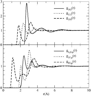
Figure 1: The pair correlation functions for water at 298 K and 1 atm, calculated with the TIP5P model.

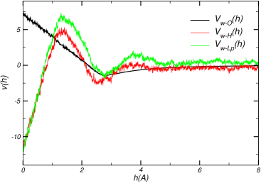
Figure 2: Measured effective potential (Units: kJ/mol) of LJ and charged sites with the ’liquid wall’ (see text).

In this MD simulation we also measured the interaction energy of a molecule located at a distance $h_{z}$>0 with all molecules contained in the semi-volume defined by $z\leq 0$. The number of water molecules in half the MD box fluctuates as a function of time (with a deviation of 2%, at STP) and our measurement corresponds then to the ($\rho$,P,T) ensemble. In Fig. 2 we include the measured effective potentials for LJ and charge - charge interactions as a funcion of the distance $h_{z}$ between the site and the origin. The Ewald constant was set equal to zero in this calculation. The histograms for LJ atom-atom interactions converge to the values of Fig. 2 after a few ps., the electrostatic interactions instead show very large fluctuations as a function of time, and the averages are over 100 ps. The measured components of the electrostatic forces along $x$ and $y$ axes show an averaged value of zero, with a deviation of less than 5% of the calculated maximum value for the $z$ component.

We found that the effective potential energies $U_{eff}(h)$ that we measured in our MD run, can be reproduced by a mean field calculation of the effective interaction potential of one molecule with a “wall” at $z=0$, but taking into account the discrete distribution of particles within the “semi-volume” at $z<0$, as given by the corresponding pair distribution function. That is,

$$U_{eff}(h)=\int_{-\infty}^{0}dz\int_{-\infty}^{\infty}dx\int_{-\infty}^{\infty}dy\,U(r)\,g_{2}(r)\,,\>\,with\,r=\sqrt{(x^{2}+y^{2}+(z+h)^{2})}$$ (1)

and the effective force is numerically calculated:

$$F_{eff}(h)=-\frac{\partial}{\partial h}U_{eff}(h)\;.$$ (2)

Where

$$U(r)=4\varepsilon[(\frac{\sigma}{r})^{12}-(\frac{\sigma}{r})^{6}]$$

for LJ interactions, and

$$U(r)=\frac{q_{i}q_{j}}{r}$$

for charge $q_{i}$ - charge $q_{j}$ interactions.

Using the pair distribution functions of Fig. 1, the $U_{eff}(h)$ and $F_{eff}(h)$ functions were numerically integrated for each pair of $site-site$ interaction. Note that, as we are dealing with a disordered sample of neutral molecules, all $g_{2}(r)$ pair correlation functions are approximately equal to 1 for $r\gtrsim 10$A, including those between charged sites (H and Lp sites of the TIP5P model). These functions are used to calculate the effective interaction of LJ sites and charges with the semi-volume at $z<0$. Therefore, in a mean field approximation, both quantities $U_{eff}(h)$ and $F_{eff}(h)$ tend to zero for large distances $h$.

     

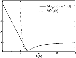
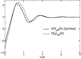
Figure 3: The effective interaction potential on (a) O (a LJ site) and (b) charged sites, located at a distance $h$ of the water semi-volume.

The following figure, Fig. 3(a) shows the interaction energy between a LJ site at a distance $h$ of the liquid surface, calculated with the pair correlation function $g_{OO}(r)$ and, for the sake of comparison, we include the same interaction potential with a homogeneous semi-volume steele . Note that both potentials greatly differ at short distances $z$. This fact is important, for example, in studies on the interaction of confined water within hydrophobic surfaces hydrophobic-surf , where a large difference will be found when performing the calculations using our effective interaction potential, instead of that given by an uniform distribution of sites. Fig. 3(b) is the result obtained for q-q interactions, calculated with the pair correlation functions $g_{HH}(r)$, $g_{LpLp}(r)$ y $g_{HLp}(r)$. The obtained $U_{eff}(h)$ functions closely follows those measured in our MD sample of pure water at STP.

III Our amphiphilic molecule model solved in water

In a next step we studied the pair distribution functions of an amphiphilic molecule solved in water. We propose two simple amphiphilic models, one is charged and the other is neutral, with a dipolar head.
Our charged amphiphilic consists in a semiflexible single chain of 14 atoms, the bond lengths are held constant, but bending and torsional potentials are included. The first two atoms of the chain mimic a charged and polar head (atom 1 with $q_{1}$ =- 2 e, atom 2 with $q_{2}$ = 1 e), sites 3 to 14 form the hydrophobic tail with uncharged atoms: sites 3 to 13 are united atom sites $CH_{2}$ and site 14 is the united atom site $CH_{3}$. This charged model is the same used in the simulation of NB films zg-bub08 and correspond to an oversimplification of sodium dodecyl sulfate SDS ($CH_{3}(CH_{2})_{11}OSO_{3}^{-}\,Na^{+}$) in solution, so we are including a $Na^{+}$ ion per chain. The LJ parameters are those of ref. zg , except for the sites 1 and 2 that form the amphiphilic polar head: $\sigma_{1}=4.0$Å, $\sigma_{2}=$4.0 Å, $\sigma_{Na}=$1.897 Å, $\varepsilon_{1}$= 2.20 kJ/mol, $\varepsilon_{2}$= 1.80 kJ/mol and $\varepsilon_{Na}$= 6.721 kJ/mol. The masses of the sites are the corresponding atomic masses, except that $m_{1}=m_{2}=48$au., in order to mimic the ’real’ amphiphilic head. The LJ parameters of the united atom sites are taken from calcutations on n-alkanes pot.toxvaerd : $\sigma_{CH2}=$3.850 Å, $\sigma_{CH3}=$3.850 Å, $\varepsilon_{CH2}$= 0.664 kJ/mol, $\varepsilon_{CH3}$= 0.997 kJ/mol. The LJ parameters for the $Na^{+}$ion are taken from simulations of SDS in aqueous solution mike-sds-miscelle and Newton black films zg .

The intramolecular potential includes harmonic wells for the bending angles $\beta$ and the usual triple well for the torsional angles $\tau$, the constants are the those commonly used for the united atom site $CH_{2}$tildesley . These potentials are needed to maintain the amphiphilic stiffness and avoid molecular collapse. The bending potential is

$$V(\beta)=k_{CCC}(\beta-\beta_{0})^{2}\;,$$

with $\beta_{0}=109.5\,deg.$ and $k_{CCC}=520\,kJ/rad^{2}$. The torsional potential is of the form

$$V(\tau)=a_{0}+a_{1}cos(\tau)+a_{2}cos^{2}(\tau)+a_{3}cos^{3}(\tau)+a_{4}cos^{4}(\tau)+a_{5}cos^{5}(\tau)\;,$$

the constants are $a_{0}=9.2789,$ $a_{1}=12.1557,$ $a_{2}=-13.1202,$ $a_{3}=-3.0597,$ $a_{4}=26.2403$ and $a_{5}=-31.4950\,kJ/mol$; this potential has a main minimum at $\tau=0\,deg.$ and two secondary minima at $\tau=\pm 120\,deg.$
The neutral amphiphilic molecule is entirely similar to the charged one, except that, in this case is $q_{1}=-q_{2}$ =- 1 e, and no ions are included in the simulation.

      

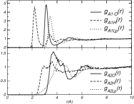
Figure 4: Pair correlation functions between the charged amphiphilic model sites, unbonded ion and water sites.

      

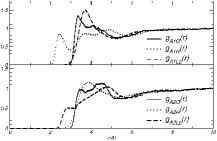
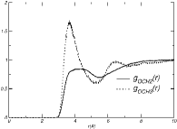
Figure 5: Pair correlation functions between the neutral amphiphilic model sites and water sites.

The pair correlation functions between the amphiphilic and the TIP5P sites were obtained from a MD simulation, performed with a time step of 1 fs, 40 ps. of equilibration, and afterwards measured over a free trajectory of 40 ps. The following figures include the pair correlation functions (Fig.4 for charged amphiphilics and Fig. 5 for neutral ones) and the corresponding effective potentials for LJ sites, (Fig. 6) and charged sites (Fig. 7), calculated as in the preceding section for both amphiphilic models, interacting with a ’liquid semi-volume’.

         

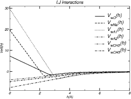
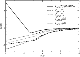
Figure 6: Effective potentials for LJ sites of (a) charged and (b) neutral amphiphilic sites interacting with the “liquid wall”. Units as in Fig. 2

         

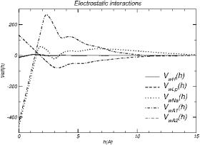
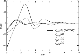
Figure 7: Effective potentials calculated for charged sites of (a) charged and (b) neutral amphiphilics interacting with the “liquid wall”. Units as in Fig. 2

IV The biological bilayer model:

Using the above mentioned molecular models we can build several simple models of biological membranes and also a Newton black film zg-bub08 . The initial configuration of our MD simulations is always a pre-assembled structure, because the time scale of self-assembly, starting from a homogeneus mixture of lipids and water, is about ns. mem-mike-coarse.grain , the order of our longest simulations. For example, Fig. 8 shows the initial configuration of one of our simple biological membrane simulations, consisting of 226 of our charged amphiphilics, 226 $Na^{+}$ ions and 2188 TIP5P molecules, the bilayer is perpendicular to the $\widehat{z}$ MD box axis, with a box size of $a=b=45.$Å, $c=$1000 Å. Although real biological membranes are usually modeled with amphiphilic molecules consisting in one head with two hydrophobic chains mem-mike-all.atom1 , here we are analysing an extremely simple membrane model in which the strong electrostatic interactions and the density of hydrophobic chains in the bilayer play the key rôle. That is our reason for using the same amphiphilic model as that in our NB films simulations zg-bub08 .

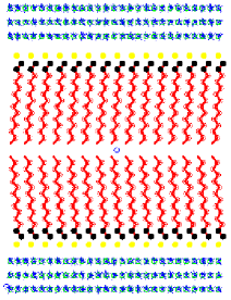
Figure 8: Initial configurations of: a model biological membrane.

The MD integration algorithms, time step and cut-off radius are essentially identical to those used on our bulk samples, except for the 2D periodic boundary conditions, that now are applied only in the xy plane of the bilayers, and that we are including: (a) an effective external potential for biological membranes (in the direction perpendicular to the bilayer) due to the surrounding water not explicitly included in the simulation, and (b) our proposed macroscopic electric field.

For our constant temperature MD simulations of bilayers we use the Berendsen algorithm berendsen1 , applying the equipartition theorem to each type of molecule and a strong coupling constant $\tau=0.5\,\Delta t$ linking the average kinetic energy of each kind of molecules (amphiphilics, ions and water) to the desired kinetic energy of $\frac{3}{2}k_{B}T_{0}$, with $T_{0}=300K$. The Berendsen algorithm turned out to attain equipartition and equilibrium temperatures faster than the Nose-Hoover chains method nose-chains (used in our bulk samples), when applied to our mix of flexible and rigid molecules.

We also have to take into account the following facts:

a) Although the $c$ parameter of the MD box is constant, at equilibrium the width of the slab (that includes the layers of amphiphilic and water molecules) fluctuates in time, mantaining a given average perpendicular pressure, which we set about 1 atm in all included simulations. If desired, by allowing variations of the ab MD box size, the lateral tension of the bilayer can also be adjusted to fluctuate around a given value.

b) To simulate a single biological membrane, all effective interactions between our molecules included in the sample and those water molecules outside the slab, we include effective potentials $U_{eff}(h)$, their contribution to the energy and forces on every site depending on the type of site and the distance of the site to both surfaces that delimit the slab. That means that at each time step we need to determine the two distances $h^{-}$ and $h^{+}$, of all molecular sites to the instant location of the two confining liquid surfaces. It is interesting to note that these effective potentials and forces tend to maintain a tight packing of the bilayer along $\widehat{z}$. This last statement was verified by running a sample similar to that of Fig. 8 (a), except that all ions and amphiphilic molecules are removed. In a few ps. the two slabs of water join in a single layer, with the final (and fluctuating) thickness corresponding to the experimental STP density of water.

c) The site-site LJ interactions between all molecules in the sample have a finite cutt-off radius of 15 A. In 3D simulatons, the contributions of sites outside this sphere are taken into account assuming an uniform distribution of sites and performing a simple integration. In our cuasi 2D system, the volume to integrate is that outside the cut-off sphere and within the volume of the slab. Appendix A in Ref. zg-bub08 includes this integral.

d) The electrostatic interactions are calculated via the standard 3D Ewald sums with a large size box along the perpendicular to the bilayer slab and 2D periodic boundary conditions in the plane of the slab. The Ewald’s sum term corresponding to our proposed macroscopic electric field is discussed in the following section.

V The macroscopic electric field in a quasi - 2 D sample:

Electrostatic forces have a far from negligible contribution to the self-assembly and final patterns found in soft matter systems. Several reviews for quasi-2D and 3D geometries ewald-2d-deleeuw ; jorge-2d ; ewald-mz are available, where the macroscopic electric field is given, in a first approximation, by the first multipolar (dipole) moment of the MD box. In particular, for monolayers, the macroscopic electric field is given in a first approximation by the contribution of the surface charges of an uniform dielectric slab. If the slab, of volume $V$, is oriented perpendicular to the z direction, the contribution to the total energy of the system is:

$U^{macrosc.}=\frac{2\pi}{V}M_{z}{{}^{2}}$,
where $M_{z}$ is the total dipole moment of the slab, and the contribution of this term to the total force on every charge $q_{i}$ of the sample is:

$F_{i}^{macrosc.}(z)=-\frac{4\pi}{V}M_{z}$.
This approximation for the macroscopic field, plus 3D Ewald sums with a large MD cell along $z$, has been tested in simulations of monolayers ewald-mz2 ; ewald-mz . In the MD simulation of bilayers, instead, and due to its geometry, the total dipole moment $M_{z}$ is zero in a time average and therefore a more accurate estimation of their macroscopic electric field is desirable.

In a recent paper zg-bub08 we discussed several approaches and proposed a novel coarse fit of the charge distribution of the different membrane components (water and amphiphilics plus ions), using a superposition of gaussian distributions along $z$. In this way, the contribution of these charge distributions to the macroscopic electric field can be exactly calculated. The method is extremely simple to implement in numerical simulations, and the spatial and temporal charge inhomogeneities are roughly taken into account.

At each time step of the MD simulation we decompose our bilayer’s charge distribution in four neutral slabs: two for the upper and lower water layers and other two for the amphiphilic heads plus ions. For each one of the four neutral slabs, instead of consider two planar surfaces with an uniform density of opposite charges, we propose two gaussian distribution along z, the perpendicular to the slabs, with the same opposite total charges and located the same relative distance (maintaining the slab width). The coarsed distribution of charges in the bilayer is then a linear superposition of gaussians:

$\rho(z)=\sum_{i}\,\frac{q_{i}}{\sqrt{2\pi}\sigma_{i}}\exp(-\frac{(z-z_{i}){{}^{2}}}{2\sigma{{}^{2}}_{i}}))\quad,$

The macroscopic electric potential $V(z)$ and the force field $E_{z}(z)$ due to this type of charge distribution can be exactly solved. In Appendix C of Ref. zg-bub08 we include the analytically solved integrals (one of them is a new integral not included in Mathematica math ). The final result is:

$V(z)=-2\sqrt{2\pi}\sum_{i}\,\sigma_{i}\,q_{i}\,(\exp(-\frac{(z-z_{i}){{}^{2}}}{2\sigma_{i}{{}^{2}}})-(\frac{z-z_{i}}{\sqrt{2}\sigma_{i}})\,Erf[\frac{(z-z_{i})}{\sqrt{2}\sigma_{i}}])\,.$

$E_{z}(z)=-\frac{\partial V(z)}{\partial z}=2\pi\sum_{i}\,q_{i}\,Erf[\frac{(z-z_{i})}{\sqrt{2}\sigma_{i}}].$

These expresions are valid for any number of slabs, that as a function of time can change not only their position and width but also they can superpose. To include the macroscopic electric field term we need to determine the values of the $\sigma_{i},$ $z_{i}$ and $q_{i}$ parameters at each MD time step. For each one of the two slabs that simulate the charge distribution of chains’ heads plus ions, we fit the $z_{i}$ parameters of two gaussians, so as to reproduce the dipolar moment of the slab. Their $\sigma_{i}$ values are obtained from the corresponding charge distributions, with $q_{i}=1$ for ions and $q_{i}=-1$ for chains’ heads. Typical values of these variables, as well as the contribution of the external potential and the macroscopic electric field to the total forces on all molecules, are reported for all simulated bilayers in section VI.

Here we have applied this exact calculation method of the macroscopic electric field to a symmetrical (along z) slab geometry, but it is also valid in an asymmetrical case, which may imply a finite difference of potential across the bilayer. As we pointed out in Ref. zg-bub08 , the extension of this method ( a coarse grained representation of the macroscopic electric field via a superposition of gaussians) to other geometries is also strightforward, a spherical geometry, for example, would be useful for the study of miscelles. Its great advantage is that these representations can be analytically solved.

VI Four calculated model bilayers, results:

To test the versatility of our approach, four different bilayers models were studied: with and without ions solved in water and with and without the water layer. We only include here a few simulations of each simplified bilayer model, which were mainly performed to analyze the contribution of the effective external potential and the macroscopic electric fields to the equilibrium structure and molecular dynamics of each bilayer. Elsewhere we will present a detailed analysis of the phase diagram of these and other bilayer models and their dependence on the amount of water and ions, the amphiphilics length, external pressure, lateral tension, etc.

VI.1 A simple biological membrane with its surrounding water and solved ions:

      

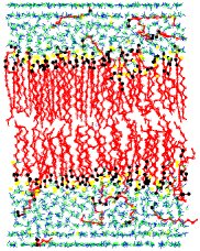
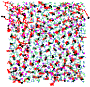
Figure 9: Final configuration of the sample of Fig. 8a, with a=b=42.45Å: (a) ac cross section, (b) ab cross section.

This is the sample whose initial configuration was included in section IV. Fig. 8(a) shows the initial and Fig. 9 the final equilibrated configuration of this simple model membrane, consisting of 226 negatively charged amphiphilic molecules, 226 positive charged ions and 2188 water molecules (9.7 water molecules per amphiphilic), the bilayer is perpendicular to the $\widehat{z}$ MD box axis, with a box size of $a=b=42.45$Å, $c=$1000 Å. In a constant volume MD simulation the final equilibrium width of this slab (including all molecules) is about 60Å. The periodic boundary conditions are applied along the $\widehat{x}$ and $\widehat{y}$ directions and a large unit cell $c$ parameter (that is, a large empty volume) is taken, in order to approximate the required 2D Ewald sums by the usual 3D sums. In addition, the contribution of the effective external potential due to the water outside the slab and the macroscopic electric field are taken into account (Fig. 10).

                        

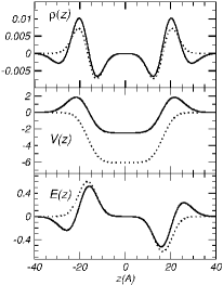
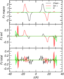
Figure 10: Profile of: (a) the macroscopic coarse fit of the charge density $\rho$(z), the macroscopic electrostatic potential V(z) and electric field E(z) (full line for total values, dotted line for heads plus ions contribution), (b) our measured profile of forces acting on all molecules due to the macroscopic electric field, the external force and total forces, as a function of the centers of mass locations along $z$, in the model membrane with charged chains.

Fig. 10 (a) shows the functions $\rho(z)$, $V(z)$ and $E_{z}(z)$ calculated in one of the time steps of the free MD trajectory of the equilibrated sample. As time evolves, these functions show small fluctuations around the values included in the figure. $\rho(z)$ is obtained from a coarse grained fit of the charge distribution of our MD sample using four charged slabs, two of them represent the charged heads plus ions and the other two the water molecules (As explained in section V). The parameters of the four slabs used to calculate $\rho(z)$ in Fig. 10 are:

$\begin{array}[]{lrrr}&q_{i}(e)&z_{i}(\textrm{\r{A}})&\sigma_{i}(\textrm{\r{A}})\\ slab\,1\,(water)&-0.241&24.515&4.705\\ &0.241&23.325&4.705\\ slab\,2\,(head\,and\,ions)&-1.0&16.349&4.011\\ &1.0&16.832&4.011\\ slab\,3\,(head\,and\,ions)&1.0&-16.832&4.011\\ &-1.0&-16.349&4.011\\ slab\,4\,(water)&0.241&-23.325&4.705\\ &-0.241&-24.515&4.705\end{array}$.

Once obtained $\rho(z)$, the macroscopic potential $V(z)$ and corresponding electric field $E_{z}(z)$ are calculated as explained in section V. Units in Fig. 10 and following ones: density of charges $\left[\rho\right]=\frac{e}{\textrm{\r{A}}^{3}}$; electrostatic potential $\left[V\right]=\frac{e}{\textrm{\r{A}}}$ (for comparison with experimental data $\left[\frac{e}{\textrm{\r{A}}}\right]=0.04803\,\frac{cm^{1/2}gr^{1/2}}{sec}=14.399\,\left[Volt\right]$ ); electric field $\left[E\right]=\frac{e}{\textrm{{\r{A}}}^{2}}$.

Most of available all-atom simulations are on bilayers of neutral amphiphilics. In our case, as the ion $Na^{+}$ is not bonded to the amphiphilic head, we cannot directly compare our results. Our model bilayer with charged amphiphilics is more similar to that calculated in Ref. mem-faraudo-07 , where a bilayer of 100 $DMPA^{2-}$ (charge=-2e) amphiphilics, 9132 water molecules and $Cl_{2}Ba$ in solution (100 $Cl^{-}$ and 150 $Ba^{2+}$ ions) is simulated. In this sample they observe a charge inversion of about 1.07 Ba(2+) ions per DMPA molecule, and therefore the contribution of lipids plus ions to the electrostatic potential is positive in the core of the bilayer, the contribution of the water layer is opposite but not large enough so as to change the sign of the total potential. Our single chain amphiphilic has a charge of $-1e$, but from the atomic density profiles of Fig. 11 we calculate that most of the ions $Na^{+}$ remain around the head group, but about 11% of them are solved in the water layer. That means that our bilayer do not show charge inversion and the contribution of lipids plus ions to the electrostatic potential is negative, and we also observe that the contribution of the water layer is opposite but not large enough so as to change the sign of the total potential. We obtain for charged head and ions a negative potential contribution of about -6 $e/\textrm{\r{A}}$, the water layer polarization is not strong enough to counterbalance this trend, and the final value is a negative potential, at the membrane core, of about -2 $e/\textrm{\r{A}}$.

This behavior is at variance with the usual one observed for neutral lipid bilayers, where a dielectric overscreening of water is observed and therefore the total calculated electrostatic potential $V(z)$ is opposite to the contribution given by the amphiphilic layers. For example, in a typical all-atom MD simulation of a neutral SDPC (1-stearoyl-2-docosahexaenoyl-sn-glycero-3-phosphocholine) phospholipid bilayer mem-electr-mike-1 , it is found that, on average, the negative P atom in the head group is located closer to the membrane interior than the positive N atom, the same orientation for charges is obtained with our coarse grained fit of the head groups plus ions. The SDPC lipid dipoles mem-electr-mike-1 are oriented so as to contribute with a negative electrostatic potential in the membrane core of about -1 V ($\sim-14.4e/\textrm{\r{A}}$), the water polarization creates an opposite potential and the total result is a positive potential of about +0.5 V mem-electr-mike-1 . A similar positive potential at the membrane core of $\sim+0.35$V is calculated in an all-atom MD simulation of a POPC (palmitoyl-oleoyl-phosphatidylcholine) lipid membrane mem-POPC and of +0.575V in other MD simulation of a DPPC (dipalmitoy-phosphatidyl-choline) bilayer mem-DPPC-berendsen .

Fig. 10 (b) includes the contribution of the effective external potentials $U_{eff}(z)$ (that models the surrounding water) and the macroscopic electric field $E_{macro}(z)$ to our measured total forces on water, ions and chain molecules, as a function of the center of mass locations along z, averaged over a free MD trajectory of 50 ps, Units: $\left[F\right]=kJ/mol/\textrm{\r{A}}$. The negatively charged amphiphilics tend to drift away of the bilayer due to the macroscopic electric field but this tendency is balanced by an opposite force on the movile ions located in the neighborhood of the charged heads. The external force due to the surrounding water is mainly felt by the molecules near the up and lower borders of the sample, although near the head groups follows the same tendency of the forces due to the macroscopic field. Lastly, when adding all molecule - molecule interactions, the total forces on the amphiphilics tend to maintain a bilayer structure.

Figs. 11(a) and (b) show, respectively, our atomic and electronic density profiles. The head to head distance, perpendicular to the bilayer, is about 36Å with an area per hydrophobic chain of $16\textrm{\r{A}}^{2}$. Our profile for the water density is similar to those calculated for all-atom samples only around the amphiphilic polar heads, but near both surfaces of the slab, our profile resembles that calculated for water interacting with a solid surface, although the fluctuations of density are smaller due to a less repulsive short range external potential (Fig. 3 (a)). The last difference is due to our restriction on the water diffusion along z and to have allowed only very small fluctuations of the internal pressure in the z direction, this in turn implies that the molecules near the up and lower border of the sample, at less than 2-3 times the LJ size of water, should not be taken into account when measuring the different bilayer properties.

      

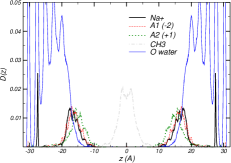
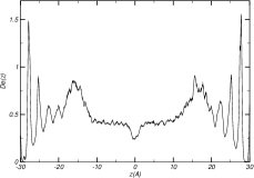
Figure 11: (a) Atomic (number of atoms per $\textrm{\r{A}}^{3}$) and (b) electronic density profiles for the sample with a=b=42.45Å.

To obtain a fast overview of how these properties depend on the amphiphilics density, we performed a small series of five constant volume - constant temperature simulations, with increasing values of ab cross section, up to $a=b=45.0$Å, at which value large amounts of water molecules interpenetrate the membrane and disorder the bilayer structure, as measured by the diffusion coefficients and the atomic density profile. In all simulations the pressure on the membrane, along z, is maintained fluctuating about 1atm., in the sample of section (42.45 Å)² the lateral pressure is about 3 atm, falling to $\sim$2 atm in the sample of section (45.0 Å)² , and the total width of the sample drops from 60Å to about 50Å.

The diffusion coeficients for the amphiphilic chains, ions and water, are highly anisotropic in all samples. For the sake of comparison, the experimental STP ($25^{\circ}$C and 1 atm.) diffusion coeficient of bulk water w-dif is $2.30\,10^{-5}cm^{2}/\sec$, and the lateral diffusion of lipids in a stack of DPPC bilayers DPPC-dif , for example, is about $\,10^{-6}cm^{2}/\sec$ at 330 K and less than $0.6\,10^{-6}cm^{2}/\sec$ at 300 K. The next Table gives our measured diffusion coeficients for amphiphilic chains, ions and water, in the xy plane and in the z direction (Units: $10^{-5}cm^{2}/sec$). It has to be taken into account that for simulation samples of our size it is necessary to perform MD runs of nanoseconds to meassure diffusion coeficients of the order of $10^{-6}cm^{2}/\sec$. As our free MD trajectories are of 100 ps, our values are an upper limit to the diffusion coeficients of these samplesbilayer-lipid-diff . In the sample of section (42.45 Ų) we measured oscillations of the centers of mass around an equilibrium position, without diffusion, and correspond to a simulation of a glassy phase, while for the sample of section (45.0 Ų) the measured difusion coefficients are of the order of $10^{-5}cm^{2}/\sec$ and correspond to a liquid phase of solved amphiphilics in water.

$\begin{array}[]{cllllll}&chain^{-}(z)&chain^{-}(xy)&ion^{+}(z)&ion^{+}(xy)&W(z)&W(xy)\\ a=42.45\textrm{\r{A}}&\>-&-&-&-&-&-\\ a=43.20\textrm{\r{A}}&\>0.2&0.7&0.15&0.6&0.2&1.2\\ a=43.50\textrm{\r{A}}&\>0.5&1.8&0.45&1.5&0.45&2.2\\ a=45.00\textrm{\r{A}}&\>1.6&3.8&1.6&3.1&1.0&3.8\end{array}$

Finally, the distortion of the amphiphilic molecules was determined by the fraction of trans to gauche (g+, g- ) torsional angles and by the distribution of site-site intramolecular distances (Fig. 12), calculated on a free MD trajectory of 100 ps. Both measurements show an increasing chain disorder for samples of lower density in the xy plane.

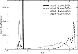
Figure 12: The head to bead 4 and head to tail site distances distributions for the amphiphilics in two samples.

$\begin{array}[]{ccc}&\quad trans&\;g+=g-\\ a=42.45\textrm{\r{A}}&\>0.88&0.06\\ a=43.2\textrm{0\r{A}}&\>0.88&0.06\\ a=43.50\textrm{\r{A}}&\>0.86&0.07\\ a=45.00\textrm{\r{A}}&\>0.66&0.17\end{array}$

VI.2 A simple biological membrane without surrounding water:

      

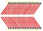
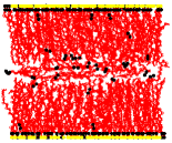
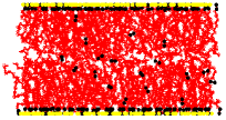
Figure 13: Simple model membrane without water: (a) initial configuration, (b) final configuration, (c) final configuration of a sample with lower amphiphilics density.

In general, the models of amphiphilic membranes without the explicit inclusion of the solvent (water) are investigated because of their simplicity and faster calculation of fenomena at the mesoscopic scale, as presented for example in Refs. farago ; mem-potextra1 ; brannigan2 where the self-assembly of bilayers is studied using simple neutral chains of 3 to 5 beads, one of them representing the head.

Here we present a model that is simple and useful at the nanoscopic scale, that includes strong electrostatic interactions, flexible chains of a more realistic number of atoms, and the LJ interaction parameters for the hydrophobic tail are those used in all atom simulations of gel or liquid phases of amphiphilics. All these facts make it a reliable model to study the properties of guest molecules confined within a biological membrane, making it possible to measure their diffusion times, uncoiling dynamics of chain molecules, interaction with head groups, etc.

Here we include a simple model bilayer consisting on 400 negatively charged chains plus 400 positive ions. We perform two MD simulations, one with a box size $a=b=56.$Å (HD sample with $16\,\r{A}^{2}$per chain), and a second one with $a=b=65$Å (LD sample with a density of $21\,\r{A}^{2}$per chain), $c=$1000 Å for both. As an example of the versatility of our model, the chains in this section consists in 20 beads, 2 of them forming the strongly charged head. Except for their length, these chains are entirely similar to those of the preceding section. As in the other cases included in this chapter, the phase diagram of this simple membrane, and their dependence on the chain lenght are currently under study. Fig. 13(a) shows the initial and 13(b) the final configuration of the HD sample, after a free MD trajectory of 100 ps, its equilibrium thickness of 52Å. Fig. 13(c) shows the final configuration of the LD sample with an equilibrium thickness of 40Å.

The MD runs are performed including the macroscopic electric field term and the external potential which simulates the surrounding water. Fig. 14 (a) shows the functions $\rho(z)$, $V(z)$ and $E_{z}(z)$ calculated in one of the time steps in the free trajectory of the equilibrated sample. In this case, $\rho(z)$ is obtained from a coarse grained fit of the charge distribution of our MD sample using only two charged slabs that represent the charged heads plus ions (As explained in section V). The parameters used to calculate the functions in Fig. 14 (a) are:

$\begin{array}[]{lrrr}&q_{i}(e)&z_{i}(\textrm{\r{A}})&\sigma_{i}(\textrm{\r{A}})\\ slab\,1\,(head\,and\,ions)&-1.0&23.592&4.352\\ &1.0&27.057&4.352\\ slab\,2\,(head\,and\,ions)&1.0&-27.057&4.352\\ &-1.0&-23.592&4.352\end{array}$

                  

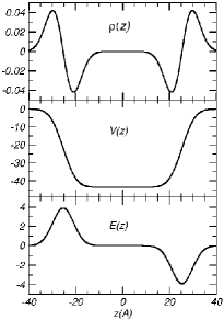
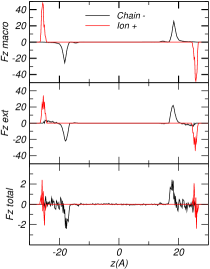
Figure 14: Profile of: (a) the macroscopic coarse fit of the charge density $\rho$(z), potential V(z) and macroscopic electric field E(z) (full line for total values, dotted line for heads plus ions contribution), (b) our measured profile of macroscopic electric field, external force and total forces acting on all molecules, as a function of the location of their centers of mass along $z$, in the model membrane without water.

In this bilayer model the potential field and forces at the core (Fig. 14 (a) and (b)) are higher than those of the preceding section, due to the large values of the charge density $\rho(z)$ and the lack of the electrostatic shield provided by the water layers.

The atomic density profiles (Fig. 15) show that the monoatomic positive ions remain at the border of the slabs, and the same happens with most of the amphiphilic heads, although for some of them we measured large excursions of the head groups within the bilayers, as shown in Fig. 13.

   

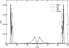
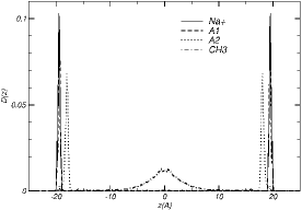
Figure 15: Atomic density profiles (number of atoms per $\textrm{\r{A}}{{}^{3}}$), (a) HD sample , (b) LD sample.

In the electron density profiles (Fig. 16) we can see that the heavier atoms remain, on average, at less than $\sim 5\textrm{\r{A}}$ of up and lower border.

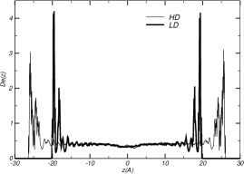
Figure 16: Electron density profile (electrons/$\textrm{\r{A}}{{}^{3}}$) for HD and LD head groups.

The distortion of the amphiphilic molecules is measured via the bending and torsional angles distribution (Fig. 17(a)) and head to bead chain distances (Fig. 17(b)). From Fig. 17(a) we estimate a 0.84 trans fraction of the torsional angles in the HD sample and a 0.74 fraction in the LD sample. Accordingly, the head to bead 4 and head to tail distances (Fig. 17(b)) have a larger spread and smaller chain length in the LD case.

            

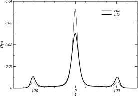
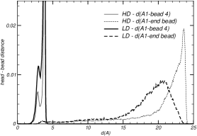
Figure 17: (a) Torsion angle distribution in the HD and LD samples. (b) The head to bead 4 and head to tail average distances for amphiphilic chains in HD and LD samples.

VI.3 Simple biological membrane with surrounding water and neutral amphiphilics:

The model membrane of this section consists of 226 neutral amphiphilics and 2188 water molecules, the bilayer is perpendicular to the $\widehat{z}$ MD box axis, with a MD box size of $a=b=42.0$Å, $c=$1000 Å. The neutral amphiphilic is that described in section III, a chain of 14 atoms where two of them model the dipolar head (atom 1 with $q_{1}$ =- 1 e, atom 2 with $q_{2}$ = 1 e), sites 3 to 14 form the hydrophobic tail. The LJ atom - atom parameters are equal in all of our amphiphilic models. In a constant volume MD simulation we found that we cannot stabilize a bilayer structure at 300K, the final sample is disordered, the water mix with the amphiphilics and we calculate an almost identical distribution of heads and end groups within the bilayer (Fig. 18). This atomic profile, the measured diffusion coeficients and molecular distortions (a trans fraction of 0.66%) indicates a large disorder in the calculated sample at 300K.

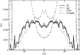
Figure 18: Atomic density profile (number of atoms per $\textrm{\r{A}}{{}^{3}}$) for the bilayer of neutral amphiphilics, without including the extra soft hydrocarbon - hydrocarbon potential interaction term.

We conclude that with this neutral amphiphilic model the electrostatic interactions are not strong enough to ensure a final bilayer structure at 300K. This problem was already found in other simulations of simple model bilayers without electrostatic interactions, as discused, for example, in Ref. mem-potextra1 .

The usual solution is to add a very soft and long ranged attractive interaction term between nonbonded hydrophobic tails farago ; mem-marcus-coarse.grain ; mem-coarse-lipowsky ; mem-potextra1 . In coarse grained membrane models without electrostatic interactions, for example, this extra interaction term between nonbonded hydrophobic beads, is crucial for stabilizing fluid bilayers. This extra potential term is usually modelled with a very soft potential of the type LJ 2-1 type instead of the usual LJ 12-6 farago ; mem-marcus-coarse.grain , or by extending the range of the 12-6 LJ potential with a flat section at the minimum mem-potextra1 , all of them show a broad atractive minimum. The obtained results suggest that this term is capable of forcing the lipid chains into gel-like conformations and tends to order the amphiphilic tails, decrease the area per head group and reduce their lateral diffusion coefficient.

For our cases of weak electrostatic interactions we decided to test the contribution of such term. Our proposed soft potential for the nonbonded united atom $CH_{2}-CH_{2},\,CH_{2}-CH_{3},\,CH_{3}-CH_{3}$ interactions is:

$\begin{array}[]{ll}V_{LJ}(r)&=4\varepsilon[(\frac{\sigma}{r})^{12}-(\frac{\sigma}{r})^{6}]\\ V_{soft}(r)&=2\varepsilon[(\frac{\sigma*0.9}{r})^{12}+Erfc\\ V_{final}(r)&=\frac{1}{2}[V_{LJ}(r)+V_{soft}(r)]\end{array}(\frac{r}{\sigma}-1)$

The idea after this proposed $V_{soft}(r)$ function can be better seen when recalling that

$\frac{\partial}{\partial r}Erfc(\frac{r}{\sigma}-1)=-\frac{2}{\sigma\sqrt{\pi}}\exp(-(\frac{r}{\sigma}-1)^{2})$,
which means a wide gaussian spread of the atractive interaction forces around $\sigma$ distances. In radial coordinates, the final interaction forces between non-bonded hydrophobic sites become:

$\begin{array}[]{ll}F_{LJ}(r)&=\frac{24\varepsilon}{r}[2(\frac{\sigma}{r})^{12}-(\frac{\sigma}{r})^{6}]\\ F_{soft}(r)&=4\varepsilon[\frac{6}{r}(\frac{\sigma*0.9}{r})^{12}-\frac{1}{\sigma\sqrt{\pi}}\exp(-(\frac{r}{\sigma}-1)^{2})\\ F_{final}(r)&=\frac{1}{2}[F_{LJ}(r)+F_{soft}(r)]\end{array}$]

Fig. 19 (a) includes the 12-6 LJ potential, the additional soft term and the final potential model, Fig. 19 (b) includes, in spherical coordinates, the corresponding forces.

      

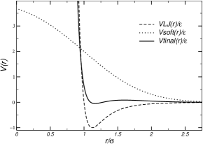
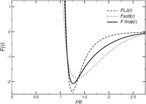
Figure 19: Proposed soft potential term (a) and forces (b) between non bonded united atoms $CH_{n}$.

A new MD run on the same sample of neutral amphiphilics, but with the addition of this soft potential term between non bonded united atoms, was performed. Fig. 20 shows the equilibrated configuration. The calculated diffusion coefficient is less than $10^{-7}cm^{2}/sec$, indicative of a gel phase. The molecular distortions, as given by the trans fraction of torsional angles is 0.85%.

            

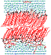
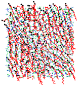
Figure 20: Final configuration for the bilayer of neutral amphiphilics, including our extra soft hydrocarbon- hydrocarbon potential interaction term.

            

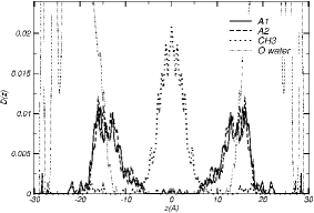
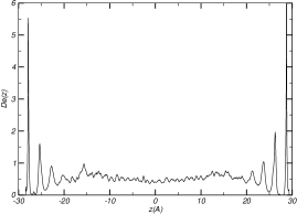
Figure 21: Atomic density profile (number of atoms per $\textrm{\r{A}}{{}^{3}}$) and electron density profile (electrons/$\textrm{\r{A}}{{}^{3}}$) for the bilayer of neutral amphiphilics, including our extra soft hydrocarbon- hydrocarbon potential interaction term.

                              

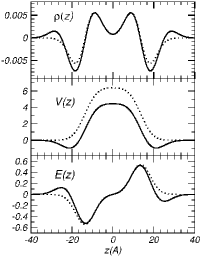
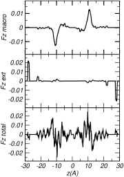
Figure 22: Profile of: (a) the macroscopic charge density $\rho$(z), potential $V(z)$ and electric field $E(z)$ (full line for total values, dotted line for heads plus ions contribution), (b) our measured profile of macroscopic electric, external and total forces on amphiphilics, as a function of the location of their centers of mass along $z$, in the model membrane of neutral amphiphilics, and including our extra soft hydrocarbon- hydrocarbon potential interaction term.

Fig. 21 includes the atomic and electronic density profile of this sample, and Fig. 22 its macroscopic electric field and forces on molecular centers of mass, as a function of $\hat{z}$, the axis perpendicular to the bilayer. Units as in the preceding sections. The macroscopic electric potential V(z) is positive in the centre of the bilayer, because, on time and spacial average, the head dipoles point to the interior of the bilayer.

This last point suggested a new MD run with model neutral amphiphilics but with a reverse dipolar moment. Therefore the last studied model membrane is entirely similar to the preceding one, except that the neutral amphiphilics have a reverse dipolar head, that is, the A1 site has a charge of +1e and site A2 has a charge of -1e. The soft potential term between non bonded united atoms is also included. The procedure and the obtained results of this case are entirely similar to those reported in this section, and we are not including them here, except for the obtained profile of the macroscopic field and the measured profile of forces on the amphiphilics as a function of the location of their centers of mass along $z$, Fig.23. The calculated macroscopic potential V(z) to that calculated, for example, in the all-atom simulation of a membrane of neutral SDPC lipids mem-electr-mike-1 , except that their negative potential is of about -14.4$e/\textrm{\r{A}}$, and ours is about -4$e/\textrm{\r{A}}$. The difference is explained by the average dipolar moment of the SDPC molecule along z, of about 0.9 $e\textrm{\r{A}}$ and ours is about 0.2$e\textrm{\r{A}}$ (due to a mean orientation angle of 82deg. with respect to the bilayer normal).

                              

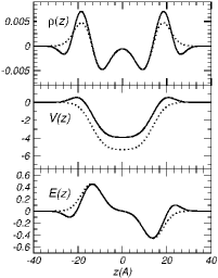
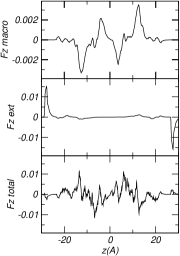
Figure 23: Profile of: (a) the macroscopic charge density $\rho$(z), potential $V(z)$ and electric field $E(z)$ (full line for total values, dotted line for heads plus ions contribution), (b) our measured profile of macroscopic electric, external and total forces on amphiphilics, as a function of the location of their centers of mass along $z$, in the model membrane of neutral amphiphilics with reverse dipole (q(A1)=1 e, q(A2)=-1 e), and including our extra soft hydrocarbon- hydrocarbon potential interaction term.

The results of the last simulation implies that by increasing the head dipolar moment of the neutral amphiphilics, the bilayer should be stable. And effectively, with a MD simulation of neutral amphiphilics, but with a strong charge of +4e on site A1 and a charge of -4e on site A2, we obtained an equilibrated bilayer sample, without the need of including the extra soft interaction term between the non-bonded hydrocarbons sites.
Most probably this is an indication that our membrane sample is not fully hydrated and a larger amount of water should be included.

VII Conclusion:

In this paper we studied several simple models of amphiphilic biological bilayers, and analyzed the key rôle of the electrostatic interactions in their self-assembly. The reverse model bilayer, a NB film was analysed in a previous paper zg-bub08 . The molecular models are simple enough so a large number of components can be included in the MD samples, but also detailed enough so as to take into account molecular charge distributions, flexible amphiphilic molecules and a reliable model of water. All these properties are essential to obtain a reliable conclusion at the nano- scale. Our amphiphilic model also allows to study, in a simple way, the properties of bilayers formed by charged or neutral amphiphilics and with or without explicity including water molecules in the numerical simulations.

As for the calculation of the electrostatic interactions, we use our proposed novel and more accurate method to calculate the macroscopic electric field in cuasi 2D geometries zg-bub08 , which can be easily included in any numerical calculation. The method, that essentially is a coarsed grain fit of the macroscopic electric field beyond the dipole order approximation, was applied here to symmetrical bilayers (along the normal to the bilayer and with periodic boundary conditions in two dimensions), but their derivation is general and valid also for asymmetrical slab geometries.

We also propose a mean field method to take into account the far distant water molecules interacting with a single bilayer of the biological type. This procedure allows the study of one isolated biological bilayer in solution, and not the usual stack of bilayers, as obtained when 3D periodic boundary conditions are applied.

Lastly, we emphasize the relevance and utility of these simple bilayer models. They can be applied to the systematic study of the physical properties of these bilayers, that strongly depend not only on ’external parameters’, like surface tension and temperature, but on the kind of guest molecules of relevance in biological and/or ambient problems embedded in them. In turn, the structure and dynamics of the embedded molecules strongly depend on their interactions with the bilayer and with the sorrounding water.

These simple model bilayers can also be useful to model, for example, the synthesis of inorganic (ordered or disordered) materials via an organic agent nanotech . This is a recent and very fast growing research field of nanotechnologycal relevance, as are lithography, etching and molding devices at the nanoscopic scale. Another fast developing field is that of electronic sensors and nanodevices supported on lipid bilayers nanotech2 ; nanotech3 . Lastly, as our model retains the flexibility of the original amphiphilics, and the electrostatic interactions are included, the approach is really useful to obtain ’realistic’ solutions to the above mentioned problems as well as those related to electric fields and electrostatic properties.

- (1) D. Chandler, Nature 437, 640 (2005).
- (2) Z. Gamba, submitted to J. Chem. Phys. (2008).
- (3) S. Bandyopadhyay, J. C. Shelley and M. L. Klein, J. Phys. Chem. B 105, 5979 (2001).
- (4) O. Farago, J. Chem. Phys. 119, 596 (2003).
- (5) I. R. Cooke and M. Deserno, J. Chem. Phys. 123, 224710 (2005).
- (6) S. O. Nielsen, C. L. Lopez, G. Srinivas and M. L. Klein, J. Phys. Cond. Matter 16, R481 (2004).
- (7) J. C. Shelley, M. Y. Shelley, R. C. Reeder, S. Bandyopadhyhay and M. L. Klein, J. Phys. Chem. B 105, 4464 (2001).
- (8) G. Srinivas, D. E. Disher and M. L. Klein, Nature Materials 3, 638 (2004).
- (9) M. Muller, K. Katsov and M. Schick, to be published in Physics Reports (2006).
- (10) S. W. Chiu, E. Jacobsson, H. Scott, J. Chem. Phys. 114, 5435 (2001).
- (11) S. E. Feller, Y. Zhang and R. W. Pastor, J. Chem. Phys. 103, 10267 (1995).
- (12) W. Im, S. Berneche and B. Roux, J. Chem. Phys. 114, 2924 (2001).
- (13) S. Senapati and A. Chandra, J. Chem. Phys. 111, 1223 (1999).
- (14) G. Mathias, B. Egwolf, M. Nonella and P. Tavan, J. Chem. Phys. 118, 10847 (2003).
- (15) M. Cossi, G. Scalmani, N. Rega and V. Barone, J. Chem. Phys. 117, 43 (2002).
- (16) Y. Levin, Rep. on Prog. in Phys. 65, 1577 (2002).
- (17) M. W. Mahoney and W. L. Jorgensen, J. Chem. Phys. 112, 8910 (2001).
- (18) M. W. Mahoney and W. L. Jorgensen, J. Chem. Phys. 114, 363 (2001).
- (19) M. Krack, A. Gambirasio and M. Parrinello, J. Chem. Phys. 117, 9409 (2002).
- (20) G. Martyna, M. L. Klein and M. Tuckerman, J. Chem. Phys. 97, 2635 (1992).
- (21) Ciccotti G., M. Ferrario and Ryckaert J. P., Mol. Phys. 47, 1253 (1982).
- (22) Z. Gamba and B. M. Powell, J. Chem. Phys. 112, 3787 (2000).
- (23) C. Pastorino and Z. Gamba, J. Chem. Phys. 115, 9421 (2001).
- (24) C. Pastorino and Z. Gamba, J. Chem. Phys. 119, 2147 (2003).
- (25) W. A. Steele, “The interaction of gases with solid surfaces”, Pergamon Press, Oxford, 1974.
- (26) D. Bratko, R. A. Curtis, H. W. Blanch and J. M. Prausnitz, J. Chem. Phys. 115, 3873 (2001).
- (27) Z. Gamba, J. Hautman, J. Shelley and M. L. Klein, Langmuir 8, 3155 (1992).
- (28) P. Padilla and S. Toxvaerd, J. Chem. Phys. 94, 5850 (1991).
- (29) J. Shelley, K. Watanabe and M. L. Klein, Int. Quantum Chem: Quantum Biol. Symp. 17, 103 (1990).
- (30) M. P. Allen and D. J. Tildesley, “Computer simulation of liquids”, Clarendon Press - Oxford (1990).
- (31) H. J. C. Berendsen, J. P. M. Postma, A. DiNola and J. R. Haak, J. Chem. Phys. 81, 3684 (1984).
- (32) S. W. de Leeuw and J. W. Perram, Mol. Phys. 37, 1313 (1979).
- (33) J. A. Hernando, Phys. Rev. A 44, 1228 (1991).
- (34) I. Yeh and M. L. Berkowitz, J. Chem. Phys. 111, 3155 (1999).
- (35) A. Brodka and A. Grzybowski, J. Chem. Phys. 117, 8208 (2002).
- (36) Web site: http://www.integrals.com, open site of Wolfram Research, Inc.
- (37) J. Faraudo and A. Travesset, Coll. and Surf. A 300, 287 (2007).
- (38) L. Saiz and M. L. Klein, J. Chem. Phys. 116, 3052 (2002).
- (39) S. K. Kandasamy and R. G. Larson, J. Chem. Phys. 125, 074901 (2006).
- (40) D. P. Tieleman and H. J. C. Berendsen, J. Chem. Phys. 105, 4871 (1996).
- (41) R. Mills, J. Phys. Chem. 77, 685 (1973).
- (42) P. Karakatsanis and T. M. Bayerl, Phys. Rev. E 54, 1785 (1996).
- (43) J. B. Klauda, B. R. Brooks and R. W. Pastor, J. Chem. Phys. 125, 144710 (2006).
- (44) G. Brannigan, P. F. Philips and F. L H. Brown, Phys. Rev. E 72, 011915 (2005).
- (45) L. Gao, J. Shillcock and R. Lipowsky, J. Chem. Phys. 126, 015101 (2007).
- (46) K. J. Edler, Phil. Trans. R. Soc. Lond. A 362, 2635 (2004).
- (47) E. T. Castellana, P. S. Cremer, Surface Science Reports 61, 429 (2006)
- (48) X. Zhou, J. M. Moran Mirabal, H. G. Craighead and P. L. McEuen, Nature Nanotech. 2, 185 (2007).