Can a primordial magnetic field originate large-scale anomalies in WMAP data?

Abstract

Several accurate analyses of the CMB temperature maps from the Wilkinson Microwave Anisotropy Probe (WMAP) have revealed a set of anomalous results, at large angular scales, that appears inconsistent with the statistical isotropy expected in the concordance cosmological model $\Lambda$CDM. Because these anomalies seem to indicate a preferred direction in the space, here we investigate the signatures that a primordial magnetic field, possibly present in the photon-baryon fluid during the decoupling era, could have produced in the large-angle modes of the observed CMB temperature fluctuations maps. To study these imprints we simulate Monte Carlo CMB maps, which are statistically anisotropic due to the correlations between CMB multipoles induced by the magnetic field. Our analyses reveal the presence of the North-South angular correlations asymmetry phenomenon in these Monte Carlo maps, and we use these information to establish the statistical significance of such phenomenon observed in WMAP maps. Moreover, because a magnetic field produces planarity in the low-order CMB multipoles, where the planes are perpendicular to the preferred direction defined by the magnetic field, we investigate the possibility that two CMB anomalous phenomena, namely the North-South asymmetry and the quadrupole-octopole planes alignment, could have a common origin. Our results, for large-angles, show that the correlations between low-order CMB multipoles introduced by a sufficiently intense magnetic field, can reproduce some of the large-angle anisotropic features mapped in WMAP data. We also reconfirm, at more than 95% CL, the existence of a North-South power asymmetry in the WMAP five-year data.

1 Introduction

The five-year data from the Wilkinson Microwave Anisotropy Probe (WMAP) (Hinshaw et al., 2008; Gold et al., 2008; Nolta et al., 2008; Dunkley et al., 2008; Komatsu et al., 2008) contain the most valuable cosmological information to study the large-scale properties of the universe (see Bennett et al. 2003a, b; Hinshaw et al. 2003a, b, 2007; Jarosik et al. 2007; Spergel et al. 2007) for previous releases of WMAP data). One of these features concerns the hypothesis that the set of temperature fluctuations of the cosmic microwave background radiation (CMB) is a stochastic realization of a random field, meaning that its angular distribution on the celestial sphere is statistically isotropic at all angular scales. Examination of the three-year WMAP data confirms highly significant departures from statistical isotropy at large angular scales (Abramo et al., 2006; Huterer, 2006; Wiaux et al., 2006; Vielva et al., 2006, 2007; Land & Magueijo, 2007; Park, Park & Gott III, 2007; Copi et al., 2007; Eriksen et al., 2007; Bernui et al., 2007), previously found also in first-year WMAP data (Tegmark, de Oliveira-Costa & Hamilton, 2003; de Oliveira-Costa et al., 2004; Hansen, Banday & Górski, 2004; Hansen et al., 2004; Copi, Huterer & Starkman, 2004; Bielewicz, Górski & Banday, 2004; Eriksen et al., 2004a, 2005; Land & Magueijo, 2005a, b; Copi et al., 2006; Bernui et al., 2006). Evidences for such large-angle anisotropy come from the asymmetry of the CMB angular correlations between the northern and southern ecliptic hemispheres (hereafter NS-asymmetry), with indications of a preferred axis of maximum hemispherical asymmetry (Hansen, Banday & Górski, 2004; Hansen et al., 2004; Bielewicz, Górski & Banday, 2004; Eriksen et al., 2004a, 2005; Land & Magueijo, 2005a, b, 2007; Bernui et al., 2006; Eriksen et al., 2007; Bernui et al., 2007). Furthermore, other manifestations of large-angle anisotropy include the unlikely quadrupole-octopole planes alignment (refering both to the strong planarity of these multipoles as well as to the alignment between such planes, see, e.g., Tegmark, de Oliveira-Costa & Hamilton 2003; de Oliveira-Costa et al. 2004; Weeks 2004; Copi et al. 2006; Wiaux et al. 2006; Abramo et al. 2006; Copi et al. 2007; Park, Park & Gott III 2007). Actually, several anomalous results were already reported after analyses of the WMAP data (Chiang et al., 2003; Vielva et al., 2004; Copi, Huterer & Starkman, 2004; Bielewicz et al., 2005; Cruz et al., 2005, 2007; McEwen et al., 2006; Bernui, Tsallis & Villela, 2006, 2007). For a different point of view see, e.g., Hajian & Souradeep (2003); Hajian, Souradeep & Cornish (2004); Donoghue & Donoghue (2005); Souradeep & Hajian (2004); Hajian & Souradeep (2005); Souradeep & Hajian (2005); Souradeep, Hajian & Basak (2006); Hajian & Souradeep (2006).

Possible sources of these anomalies include non-CMB contaminants, like residual foregrounds (Eriksen et al., 2004b; Wibig & Wolfendale, 2005; de Oliveira-Costa & Tegmark, 2006; Cruz et al., 2006; Abramo, Sodré & Wuensche, 2006; Chiang et al., 2007; López-Corredoira, 2007), incorrectly subtracted dipole and/or dynamic quadrupole terms (Copi et al., 2006; Helling et al., 2006; Copi et al., 2007), or systematic errors (Schwarz et al., 2004; Bunn et al., 2007). For this, particular efforts have been done by the WMAP team in last releases in order to improve the data processing by minimizing the effects of foregrounds (mainly coming from diffuse Galactic emission and astrophysical point-sources), artifacts (in the mapmaking process, in the instrument characterization, etc.), and systematic errors (Jarosik et al., 2007; Hinshaw et al., 2008; Gold et al., 2008). As a result, the data released by the WMAP team include the Internal Linear Combination (hereafter ILC-5yr) full-sky CMB map suitable for large-angle temperature fluctuations studies (Hinshaw et al., 2007, 2008; Nolta et al., 2008). Here we investigate the ILC-5yr map, and for completeness, we also study the other full-sky cleaned CMB maps that were differently processed from WMAP five- and three-year data releases in order to account for foregrounds and systematics. Thus, we also consider the Kim-Naselsky-Christensen (Kim, Naselsky & Christensen, 2008), WMAP-3yr ILC (Hinshaw et al., 2007), de Oliveira-Tegmark (de Oliveira-Costa & Tegmark, 2006), and Park-Park-Gott (Park, Park & Gott III, 2007) CMB maps, hereafter termed the HILC-5yr, ILC-3yr, OT-3yr, and PPG-3yr, respectively.

A number of studies has been done looking for physical explanations of the above mentioned anomalies, specially searching for a unifying mechanism relating both the NS-asymmetry and the CMB lower multipoles alignment (see, e.g., Wiaux et al. 2006; Rakic & Schwarz 2007; Dvorkin, Peiris & Hu 2007). Additionally, some processes that breaks down statistical isotropy during the inflationary epoch have been suggested (Gordon et al., 2005; Gümrükçüoğlu, Contaldi & Peloso, 2007; Pullen & Kamionkowsi, 2007; Ackerman, Carrol & Wise, 2007). Nonetheless, one can also interpret such CMB large-angle anisotropy as being of cosmological origin, in this sense globally axisymmetric space-times have been proposed to account for the mapped preferred axis in WMAP maps (Aurich, Lustin & Steiner, 2005; Hipólito-Ricaldi & Gomero, 2005; Land & Magueijo, 2006; Jaffe et al., 2006; Cresswell et al., 2006; Gosh, Hajian & Souradeep, 2007). Previous works investigated the effects of a primordial homogeneous magnetic field on the CMB temperature fluctuations on all angular scales (see, e.g., Durrer, Kahniashvili & Yates 1998; Demiański & Doroshkevich 2007). Here we study such primordial field as a possible physical mechanism to produce two large-angle phenomena, that is, the CMB NS-asymmetry and the lower CMB multipoles alignment.

In section 2 we present this primordial magnetic field scenario, and show the effect of such a field on the CMB temperature fluctuations. Then, in order to reveal such effects on simulated CMB maps we develop a geometrical-statistical method, which is presented in section 3. After that we use our anisotropic indicator to perform, in section 4, the analyses of both sets of data, the Monte Carlo simulated CMB maps as well as the WMAP maps. At the end, in section 5, we discuss our results and formulate our conclusions.

2 Primordial magnetic fields scenario

There is strong observational evidence for the presence of large-scale intergalactic magnetic fields of fews $\mu G$, and magnetic fields of similar strength within clusters of galaxies (see, e.g., Krause, Beck & Hummel 1989; Wolfe, Lanzetta & Oren 1992; Clarke, Kroenberg & Boehringer 2001; Widrow 2002; Xu et al. 2006). Nowadays it is believed that these magnetic fields are amplifications of small primordial magnetic fields of the order of few nanoGauss, that would have occured due to different processes, like galactical dynamo (see, e.g., Parker 1971; Vainshtein & Ruzmaikin 1972; Vainshtein & Zel’dovich 1972), during anisotropic protogalactic collapses, or due to differential rotation in galaxies (see, e.g., Piddington 1970; Kulsrud & Anderson 1992). In turn, such primordial seeds of magnetic fields would have several origins, for instance an electroweak phase transition (Vachaspati, 1993; Kibble & Vilekin, 1995; Baym, Bodeker & McLerran, 1996) or quark-hadron phase transition (see, e.g., Quashnock, Loeb & Spergel 1989; Cheng & Olinto 1994). Here, we assume the existence of a primordial homogeneus magnetic field and investigate their effects on the CMB temperature fluctuations at large-angles.

According to the Einstein equations for linearized metric perturbations, in absence of a magnetic field, the vector metric perturbations go like $a^{-2}$ and the velocity induced by these perturbations goes like $a^{-1}$ (where $a$ is the scale factor that accounts for the expansion of the universe). Therefore, they decay very fast with the expansion of the universe (Mukhanov, 2005) and the velocities produced by vector metric perturbations do not contribute significatively to the CMB temperature fluctuations.

The presence of a homogeneus magnetic field in the early universe change this scenario because such fields modify the behavior of charged particles in the primordial plasma via Lorentz forces producing additional velocity gradients in the fluid. In this way, a magnetic field induces Alfvén waves in the primordial plasma that propagate at velocity $v_{\mbox{\rm\footnotesize A}}$, changing the speed of sound in the photon-baryon fluid as $c^{2}_{s}\longrightarrow c^{2}_{s}+v^{2}_{\mbox{\rm\footnotesize A}}\cos^{2}\theta$, where (Adams et al., 1996)

$$v_{\mbox{\rm\footnotesize A}}^{2}=\frac{B^{2}_{0}}{4\pi(\rho+p)}\,,$$ (1)

with $\rho$ and $p$ being the density and pressure in the radiation dominated era, respectively, $B_{0}$ is the strength of the magnetic field B, $\theta$ is the angle between B and the $\vec{k}$-mode of the Fourier expansion of Alfvén velocity $v_{\mbox{\rm\footnotesize A}}$. These Alfvén wave modes induce small rotational velocity perturbations which, for the scales of our interest, have the form $\vec{v}\,\approx\,\vec{v}_{0}\,v_{\mbox{\rm\footnotesize A}}\,k\,t\,\cos\theta$, where $t$ is the cosmic time, $k\equiv|\vec{k}|$, and $\vec{v}_{0}$ is the initial velocity, which we assume to have a power spectrum of the form (Durrer, Kahniashvili & Yates, 1998; Chen et al., 2004)

$$\langle v_{0i}\,v_{0j}\rangle\propto k^{n}\,(\delta_{ij}-k_{i}\,k_{j})\,.$$ (2)

Vectorial contributions to CMB temperature fluctuations are present via Doppler and Sachs-Wolfe effects (Durrer, Kahniashvili & Yates, 1998)

$$\frac{\delta T}{T}(\hat{n})^{\mbox{(\footnotesize vec)}}\,=\,-\vec{V}_{T}\cdot\hat{n}|^{t_{0}}_{t_{\rm\small dec}}\,+\,\int^{t_{0}}_{t_{\rm\small dec}}\dot{\vec{\nu}}\cdot\hat{n}\,dt\,,$$ (3)

where $\hat{n}$ indicates any direction in the sky, $\vec{V}_{T}=\vec{V}+\vec{v}$, $\vec{\nu}$ is the vectorial metric perturbation, $\vec{V}$ is the velocity produced by $\vec{\nu}$, and the integration is between the actual time $t_{0}$ and the decoupling time $t_{\rm\small dec}$. Thus, only the rotational velocity perturbations $\vec{v}$ contributes effectively to temperature fluctuations because $\vec{\nu}$ and $\vec{V}$ decay quickly with the expansion of the universe (Mukhanov, 2005). Therefore, the signatures of a homogeneus primordial magnetic field B on the CMB temperature fluctuations are (Durrer, Kahniashvili & Yates, 1998)

$$\frac{\delta T}{T}^{\textbf{B}}(\hat{n},k)\,\approx\,\hat{n}\cdot\vec{v}_{0}\,v_{A}\,k\,t_{\rm\small dec}\,\cos\theta\,.$$ (4)

As we can see, the existence of a preferred direction associated to B affects the CMB temperature fluctuations through the angle $\theta$, which implies, a straight dependence on the orientation of the vector B, consequently, a break down of the statistical isotropy in the CMB sky.

The most suitable quantity to simulate statistically anisotropic CMB skies is the correlation matrix of multipole coefficients. For this, we expand the sky temperature fluctuations in spherical harmonics

$$\frac{\delta T}{T}(\hat{n}) = \sum_{\ell,m}a_{\ell m}Y_{\ell m}(\hat{n})\,,$$ (5)

$$a_{\ell m} = \int\frac{\delta T}{T}(\hat{n})\,Y^{\ast}_{\ell m}(\hat{n})\,d\Omega\,,$$ (6)

and then use eqs. (2), (4) and (5) to calculate the correlation matrix $\langle a_{\ell m}a^{\ast}_{\ell^{\prime}m^{\prime}}\rangle$. In this work we assume a scale-invariant power spectrum for the magnetic field, i.e., $n=-5$ in the eq. (2).

The explicit calculation of the correlation matrix elements, for a Harrison-Zel’dovich scale-invariant power spectrum for the magnetic field, gives (Durrer, Kahniashvili & Yates, 1998; Chen et al., 2004; Naselsky & Kim, 2008)

$$\langle a_{\ell m}a^{\ast}_{\ell^{\prime}m^{\prime}}\rangle^{\textbf{B}}\!=\!\delta_{mm^{\prime}}[\delta_{\ell\ell^{\prime}}C^{\textbf{B}}_{\ell m}+(\delta_{\ell+1,\ell^{\prime}-1}+\delta_{\ell-1,\ell^{\prime}+1})D^{\textbf{B}}_{\ell m}],\!\!\!$$ (7)

where

$$C^{\textbf{B}}_{\ell m}\,=\,27.12\times 10^{-16}\left(\frac{B_{0}}{1\,nG}\right)^{4}\times$$

$$\frac{2\ell^{4}+4\ell^{3}-\ell^{2}-3\ell+6m^{2}-2\ell m^{2}-2\ell^{2}m^{2}}{(\ell+2)(\ell+1)\ell(\ell-1)(2\ell-1)(2\ell+3)}\,,$$ (8)

and

$$\frac{D^{\textbf{B}}_{\ell m}}{C^{\textbf{B}}_{\ell m}}=\frac{9\pi}{32}\frac{\sqrt{(\ell+m+1)(\ell-m+1)(\ell+m)(\ell-m)}}{2\ell^{4}+4\ell^{3}-\ell^{2}-3\ell+6m^{2}-2\ell m^{2}-2\ell^{2}m^{2}}\times$$

$$\frac{\sqrt{(2\ell-1)(2\ell+3)}(\ell-1)(\ell+2)}{(2\ell+1)}\,,\hskip 28.45274pt$$ (9)

noticing that $B_{0}$ is given in nanoGauss ($nG$). Thus, the computation of the correlation matrix leads to non-zero elements of the type $(\ell,m)=(\ell^{\prime},m^{\prime})$ and $(\ell,m)=(\ell^{\prime}\pm 2,m^{\prime})$, while all the other elements are zero. In other words, the multipole matrix correlation is non-diagonal which is an inheritance of its angular dependence on $\theta$ and $\vec{v}_{0}$, shown in the eq. (4), and this fact being a consequence of the presence of the magnetic field at early times. In this scenario, correlations appear between different scales, like $\ell$ and $\ell\pm 2$, and then the multipole coefficients $a_{\ell m}$ at such scales are correlated. For this reason, one concludes that large-angle anisotropy features should appear in the CMB maps produced by this primordial magnetic field. If we consider a magnetic field in a $\Lambda$CDM universe the correlation matrix will be

$$\langle a_{\ell m}a^{\ast}_{\ell^{\prime}m^{\prime}}\rangle\,=\,\langle a_{\ell m}a^{\ast}_{\ell^{\prime}m^{\prime}}\rangle^{\mbox{\footnotesize$\Lambda$CDM}}+\langle a_{\ell m}a^{\ast}_{\ell^{\prime}m^{\prime}}\rangle^{\textbf{B}}\,,$$ (10)

where

$$\langle a_{\ell m}a^{\ast}_{\ell^{\prime}m^{\prime}}\rangle^{\mbox{\footnotesize$\Lambda$CDM}}\,=\,C^{\mbox{\footnotesize$\Lambda$CDM}}_{\ell}\,\delta_{mm^{\prime}}\,\delta_{\ell\ell^{\prime}}\,.$$ (11)

We observe that correlations between temperature fluctuations do not only depend on the angular separation between two points, but also on their orientation with respect to the magnetic field, that is, $m$-dependence. This $m$-dependence, caused by the fact that $B_{0}\neq 0$, means that now the CMB temperature fluctuations are actually statistically anisotropic.

Our purpose here is just to illustrate the effect induced by these large-angle anisotropies in CMB maps, and compare them with those features found in the CMB maps from WMAP. To study the relationship between low-$\ell$ (i.e., from $\ell=2$ to $\ell=10$) anomalies in such anisotropic magnetic field scenario, we produce, according to eqs. (7)–(11), five sets (with different strengths $B_{0}$) of Monte Carlo simulated CMB maps. For the statistically isotropic part (that is, the first term in eq. (10)) we use the CMBFAST tool to calculate the angular power spectrum $C^{\Lambda\mbox{\sc cdm}}_{\ell}$, and after that we use Cholesky decomposition of the matrix (10) in order to deal with the non-diagonality. Then we randomically simulate the $a_{\ell m}$ coefficient sets and from them we generate the CMB temperature fluctuations maps. The simulations were performed for magnetic fields intensities $B_{0}=(20\pm 10)\,nG$, to be in agreement with known limits at cosmological scales for the $n=-5$ power spectrum (see, e.g., Barrow, Ferreira & Silk 1997; Chen et al. 2004; Naselsky & Kim 2008, and Kahniashvili, Maravin & Kosowsky 2008 for other power spectrum indices).

3 The 2PACF and the Sigma-Map method

Our method to investigate the large-scale angular correlations in CMB temperature fluctuations maps consists in the computation of the 2-point angular correlation function (2PACF) (Padmanabhan, 1993) in a set of spherical caps covering the celestial sphere.

Let $\Omega_{\gamma_{0}}^{J}\equiv\Omega(\theta_{J},\phi_{J};\gamma_{0})\subset{\cal S}^{2}$ be a spherical cap region on the celestial sphere, of $\gamma_{0}$ degrees of aperture, with vertex at the $J$-th pixel, $J=1,\ldots,N_{\mbox{\footnotesize caps}}$, where $(\theta_{J},\phi_{J})$ are the angular coordinates of the $J$-th pixel’s center. Both, the number of spherical caps $N_{\mbox{\footnotesize caps}}$ and the coordinates of their centers $(\theta_{J},\phi_{J})$ are defined using the HEALPix pixelization scheme (Górski et al., 2003). The union of the $N_{\mbox{\footnotesize caps}}$ spherical caps covers completely the celestial sphere ${\cal S}^{2}$.

Given a pixelized CMB map, the 2PACF of the temperature fluctuations $\delta T$ corresponding to the pixels located in the spherical cap $\Omega_{\gamma_{0}}^{J}$ is defined by (Padmanabhan, 1993)

$$\mbox{\rm C}(\gamma)^{J}\equiv\langle\,\delta T(\theta_{i},\phi_{i})\delta T(\theta_{i^{\prime}},\phi_{i^{\prime}})\,\rangle\,,$$ (12)

where $\cos\gamma=\cos\theta_{i}\cos\theta_{i^{\prime}}+\sin\theta_{i}\sin\theta_{i^{\prime}}\cos(\phi_{i}\!-\!\phi_{i^{\prime}})$, and $\gamma\in(0,2\gamma_{0}]$ is the angular distance between the $i$-th and the $i^{\prime}$-th pixels centers. The average $\langle\,\,\rangle$ in the above equation is done over all the products $\delta T(\theta_{i},\phi_{i})\delta T(\theta_{i^{\prime}},\phi_{i^{\prime}})$ such that $\gamma_{k}\equiv\gamma\in((k-1)\delta,\,k\delta]$, for $k=1,...,N_{\mbox{\footnotesize bins}}$, where $\delta\equiv 2\gamma_{0}/N_{\mbox{\footnotesize bins}}$ is the bin-width. We denote by $\mbox{\rm C}_{k}^{J}\equiv\mbox{\rm C}(\gamma_{k})^{J}$ the value of the 2PACF for the angular distances $\gamma_{k}\in((k-1)\delta,\,k\delta]$. Define now the scalar function $\sigma:\Omega_{\gamma_{0}}^{J}\subset{\cal S}^{2}\mapsto{\Re}^{+}$, for $J=1,\ldots,N_{\mbox{\footnotesize caps}}$, which assigns to the $J$-cap, centered at $(\theta_{J},\phi_{J})$, a real positive number $\sigma_{J}\equiv\sigma(\theta_{J},\phi_{J})\in\Re^{+}$. The most natural way of defining a measure $\sigma$ is through the variance of the $\mbox{\rm C}_{k}^{J}$ function (Bernui et al., 2007),

$$\sigma^{2}_{J}\equiv\frac{1}{N_{\mbox{\footnotesize bins}}}\sum_{k=1}^{N_{\mbox{\footnotesize bins}}}(\mbox{\rm C}_{k}^{J})^{2}\,\,.$$ (13)

To obtain a quantitative measure of the angular correlations in a CMB map, we cover the celestial sphere with $N_{\mbox{\footnotesize caps}}$ spherical caps, and calculate the set of sigma values $\{\sigma_{J},\,J=1,...,N_{\mbox{\footnotesize caps}}\}$ using the eq. (13). Associating the $J$-th sigma value $\sigma_{J}$ to the $J$-th pixel, for $J=1,\ldots,N_{\mbox{\footnotesize caps}}$, one fills the celestial sphere with positive real numbers, and according to a linear scale (where $\sigma^{\mbox{\footnotesize minimum}}\rightarrow blue$, $\sigma^{\mbox{\footnotesize maximum}}\rightarrow red$), one converts this numbered map into a coloured map: this is the sigma-map. Finally, we find the multipole components of a sigma-map by calculating its angular power spectrum. In fact, given a sigma-map one can expand $\sigma=\sigma(\theta,\phi)$ in spherical harmonics: $\sigma(\theta,\phi)=\sum_{\ell,\,m}A_{\ell\,m}Y_{\ell\,m}(\theta,\phi)$. Then the set of values $\{S_{\ell},\,\ell=1,2,...\}$, where $S_{\ell}\equiv(1/(2\ell+1))\sum_{m={\mbox{\small-}}\ell}^{\ell}\,|A_{\ell\,m}|^{2}$, give the angular power spectrum of the sigma-map.

A power spectrum $S_{\ell}^{\mbox{\footnotesize WMAP}}$ of a sigma-map computed from a given WMAP map, provides quantitative information about large-angle anisotropy features of such a CMB map when compared with the mean of sigma-map power spectra obtained from Monte Carlo CMB maps produced under the statistical isotropy hypothesis. As we shall see, the sigma-map analysis is able to reveal large-angle anisotropies such as the NS-asymmetry.

4 Data analyses and results

Now we shall apply the sigma-map method to scrutiny the large-angle correlations present in the WMAP maps, and perform a quantitative comparison with the result of a similar analysis performed in sets of simulated Monte Carlo (MC) CMB maps. These sets of simulated maps are produced according to the primordial magnetic field scenario discussed above, where we consider five cases, for an equal number of values for the parameter $B_{0}$, to examine the influence of the field intensity on the CMB angular correlations. These analyses let us to test the hypothesis that the anomalous angular correlations found in the WMAP data could be explained by the presence of a magnetic field acting in the decoupling era. The WMAP data under investigation are the full-sky cleaned CMB maps derived from WMAP five- and three-year releases, namely the ILC-5yr, HILC-5yr, ILC-3yr, OT-3yr, and PPG-3yr CMB maps. Because we are interested in understand the possible cause-effect relationship between a primordial magnetic field and the large-angle anomalies mapped in CMB WMAP data, we concentrate our study on the low-order multipoles range $\ell=2-10$.

For our analyses we produce five sets of $1\,000$ MC CMB maps each, corresponding to the cases when $B_{0}=0,\,10,\,15,\,20$, and $30\,nG$. The case $B_{0}=0$ means that the MC maps were generated using a pure $\Lambda$CDM angular power spectrum seed (Spergel et al., 2007; Komatsu et al., 2008), and this case refers to the statistically isotropic CMB maps.

For $B_{0}\neq 0$ the simulated MC CMB maps were produced considering the two contributions to the random $a_{\ell m}$-modes according to eq. (10), that is, the statistically isotropic part plus the component due to the magnetic field. As a result of this, the mean angular power spectra of each set of MC maps, for $B_{0}=10,\,15,\,20,\,30\,nG$, satisfies the Sachs-Wolfe plateau effect. However, due to the contributions $\langle a_{\ell m}a^{\ast}_{\ell^{\prime}m^{\prime}}\rangle^{\textbf{B}}$ (see the second term in eq. (10)) the plateau of these mean angular power spectra are shifted upwards, where the value of such shifts is proportional to $B_{0}$. In order to compare features obtained, through the sigma-map method, from MC maps with power spectra that be consistent with the $\Lambda$CDM power spectrum we normalize the MC power spectra corresponding to the $B_{0}\neq 0$ cases. The normalized mean angular power spectra $C_{\ell}$ of these four sets of MC maps $B_{0}\neq 0$ cases and the angular power spectrum of the $\Lambda$CDM model, plus its cosmic variance limits, are shown in figure 1.

In our simulations we have assumed that the magnetic field is pointing in the South Galactic Pole–North Galactic Pole (SGP–NGP) direction. Notice that all the sky maps plotted here are in galactic coordinates, which means that the equator of the map corresponds to the Galactic plane, and the axis SGP–NGP is perpendicular to this plane.

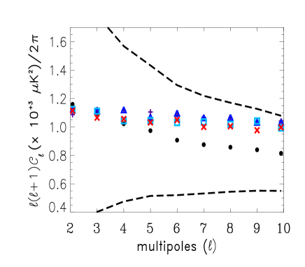
Figure 1: Normalized mean angular power spectra of the MC CMB maps used to produce the sigma-maps-MC. The bullet, plus, triangle, square, and $\times$ symbols represent the data when $B_{0}=0,\,10,\,15,\,20,\,30\,nG$, respectively. The dashed lines are the cosmic variance limits of the $\Lambda$CDM (i.e., $B_{0}=0$) power spectrum case. Note that the four sets of MC maps with $B_{0}\neq 0$ have their angular power spectra consistent with the $\Lambda$CDM case.

The data analyses consist on the following steps. For each MC temperature map we compute its corresponding sigma-map (hereafter called sigma-map-MC), and then we calculate its angular power spectrum $\{S_{\ell},\ell=1,2,...\}$. The statistical significance of the sigma-map angular power spectra computed from WMAP data (hereafter called sigma-map-WMAP) comes from the comparison with the five sets of 1 000 angular power spectra obtained from the sigma-maps-MC. To illustrate the effect of the magnetic field in the CMB low-order multipoles in MC maps, we show three cases in figure 2: the mean of 100 sigma-maps-MC obtained from a similar number of MC computed considering the statistically isotropic case $B_{0}=0$ (top), and considering magnetic field intensities $B_{0}=10\,nG$ (middle) and $B_{0}=30\,nG$ (bottom) respectively. In figure 3 instead, we show three sigma-maps with large value of the dipole term $S_{1}$, indicative of the hemispherical asymmetry phenomenon, produced from the ILC-5yr map (top) and from MC CMB maps with different magnetic field intensities: $B_{0}=10\,nG$ (middle) and $B_{0}=30\,nG$ (bottom).

Figure 2: These sky maps, in Galactic coordinates and from top to bottom, represent the mean of 100 sigma-maps-MC obtained from a similar number of MC computed considering three cases: $B_{0}=0$, $B_{0}=10\,nG$, and $B_{0}=30\,nG$, respectively, and with the magnetic field pointing in the SGP–NGP direction, which means that the equator is the preferred plane. Notice that for $B_{0}\neq 0$ the region around the equator concentrates strong angular correlations, here represented by the intense and large red sky patches.

Figure 3: For illustration we show three sigma-maps: the sigma-map-WMAP from the ILC-5yr CMB map (top), and two sigma-maps-MC having large dipole term $S_{1}$ one obtained from a MC map with $B_{0}=10\,nG$ (middle) and the other obtained from a MC map with $B_{0}=30\,nG$ (bottom).

In figure 4 we present the results of the sigma-maps spectra analyses. We observe that the sigma-maps-WMAP, obtained from the ILC-5yr, HILC-5yr, ILC-3yr, OT-3yr, and PPG-3yr CMB maps, reveal a dipole moment $S_{1}^{\mbox{\sc wmap}}$ larger than 95% of the values $S_{1}^{\mbox{\sc mc}-\Lambda\mbox{\sc cdm}}$, corresponding to sigma-maps-MC obtained from statistically isotropic CMB maps. This fact indicates that the NS-asymmetry phenomenon is present in WMAP data at 95% CL. However, we also observe in figure 4 that the angular power spectra of the sigma-maps-MC varies with the magnetic field intensity, thus to larger values of $B_{0}$ correspond sigma-maps-MC with larger values of the terms $S_{1}$ (dipole), $S_{2}$ (quadrupole), $S_{3}$ (octopole), etc. In other words, a larger value of $B_{0}$ produces a stronger hemispherical asymmetry in the MC CMB maps. Therefore, we conclude that for sufficiently large $B_{0}$, one can interpret the spectra resulting from sigma-maps-WMAP as being not anomalous at all, but consistent with those CMB temperature maps produced according to the primordial magnetic field scenario. Interestingly, simulations seems to indicate that an intensity of $B_{0}\sim 15\,nG$ is enough to have a NS-asymmetry as strong as WMAP data (see figure 4).

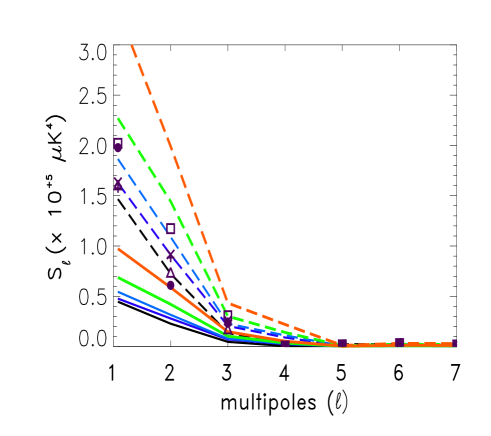
Figure 4: Angular power spectra of the sigma-maps-MC for MC produced with different magnetic fields intensities together with the sigma-maps-WMAP spectra. The plus, square, $\times$, bullet, and triangle symbols represent the data from the ILC-5yr, HILC-5yr, ILC-3yr, PPG-3yr, and OT-3yr CMB maps, respectively. From bottom to top, the solid (dashed) lines represent the mean (95% CL) values computed from the set of sigma-maps-MC corresponding to the cases $B_{0}=0,\,10,\,15,\,20,\,30\,nG$, respectively.

The effect of the magnetic field on the set of $(\ell,\,m)$-modes, for a given multipole $\ell$, deserves a close inspection. We know that in the statistically isotropic case the power of the $\ell$-multipole in a CMB map, given by $C_{\ell}=(1/2\ell+1)\sum_{m=-\ell}^{\ell}|a_{\ell m}|^{2}$, is uniformly distributed between the $(2\ell+1)$ modes, for $m=-\ell,...0,...\ell$. However, when a primordial magnetic field is acting on the CMB, and pointing in the SGP-NGP direction, we expect a non-uniform distribution of such power with a net predilection for the planar modes perpendicular to this axis, event that is termed the $m=\ell$-preference.

To investigate if the multipoles of our MC are experiencing this planarity phenomenon when $B_{0}\neq 0$, we perform a probabilistic analysis of how the power of the quadrupole moment $C_{2}$ and octopole moment $C_{3}$ are distributed in their $(2\ell+1)=5$ and $(2\ell+1)=7$ modes, respectively. For this, as a criterium for measuring the predilection for the $(\ell,m)$-mode we consider those values obtained for the quadrupole and octopole from the ILC-5yr CMB map, that is, $(\ell,m)$ is a preferred mode when it takes more than 35% of the power of such multipole, i.e., $|a_{\ell m}|^{2}+|a_{\ell m}^{\ast}|^{2}>0.35\,(2\ell+1)\,C_{\ell}$. Given a subset of MC where the power of at least one of their $(2\ell^{\prime}+1)$-modes, of a given $\ell^{\prime}$-multipole, is greater than $0.35\,(2\ell^{\prime}+1)\,C_{\ell^{\prime}}$, we define ${\cal P}_{\ell^{\prime}m^{\prime}}$ as the probability that the mode $(\ell^{\prime},m^{\prime})$ satisfies the power distribution criterium (PDC): $|a_{\ell^{\prime}m^{\prime}}|^{2}+|a_{\ell^{\prime}m^{\prime}}^{\ast}|^{2}>0.35\,(2\ell^{\prime}+1)\,C_{\ell^{\prime}}$. For instance, ${\cal P}_{2,2}$ is the probability that the quadrupolar mode $(\ell^{\prime},m^{\prime})=(2,2)$ satisfies $|a_{2,2}|^{2}+|a_{2,2}^{\ast}|^{2}>(0.35)\,(5)\,C_{2}$, where such probability is computed considering the subset of MC where at least one of the 5 modes $(\ell^{\prime},m^{\prime})$, for $\ell^{\prime}=2$ and $m^{\prime}=-2,-1,0,1,2$, has power greater than $(0.35)\,(5)\,C_{2}$. We perform a comparative analysis for two sets of MC data, namely the set of 1 000 MC $\Lambda$CDM (i.e., $B_{0}=0$, hereafter MC-$\Lambda$CDM) and the set of 1 000 MC produced with $B_{0}=20\,nG$ (hereafter MC-B20).

Additionally, to realize a possible correlation between the quadrupole-octopole planes alignment and the NS-asymmetry phenomena we also investigate the occurrence of the $m=\ell$-preference in three subsets of the MC-$\Lambda$CDM and MC-B20 sets, namely those subsets that satisfies the PDC for the quadrupole and the octopole simultaneously and such that their corresponding sigma-maps-MC have: (i) any dipole moment value $S_{1}^{\mbox{\sc mc}}$, hereafter denoted by MC-$\Lambda$CDM 0-SD and MC-B20 0-SD subsets, respectively; (ii) dipole moment value $S_{1}^{\mbox{\sc mc}}$ larger than the mean value plus one standard deviation, hereafter these data are termed MC-$\Lambda$CDM 1-SD and MC-B20 1-SD, respectively; (iii) dipole moment value $S_{1}^{\mbox{\sc mc}}$ larger than the mean value plus two standard deviations, hereafter these data are termed MC-$\Lambda$CDM 2-SD and MC-B20 2-SD, respectively. The fraction of MC, in the MC-$\Lambda$CDM and MC-B20 sets, that satisfies the above PDC for the quadrupole and the octopole simultaneously is $\sim 0.63$ for all these data subsets.

Our results for these computations are shown in Table 1, where we observe the following results. First, as expected for the three sets of MC-$\Lambda$CDM data, the analysis reveals that the quadrupole and the octopole have their power uniformly distributed between all the $(\ell,m)$-modes. Second, regarding the MC-B20 data sets, it is observed a weak preference for the $(\ell,m)\neq(\ell,0)$ modes in 0-SD and 1-SD data sets, while the planarity or $m\!=\!\ell$-preference is actually evident in the set 2-SD. Due to this fact, and according to the definition of ${\cal P}_{\ell m}$, we conclude that there is a net correlation between the quadrupole-octopole planes alignment (represented by the $m=\ell$-preference through the large values of ${\cal P}_{2,2}$ and ${\cal P}_{3,3}$) and the NS-asymmetry phenomena (represented by the fact that these large probability values appear only considering those MC that produce sigma-maps-MC with the largest dipoles $S_{1}^{\mbox{\sc mc}}$). We understand this $m=\ell$-preference as a consequence of the planarity induced by the preferred direction settled by the magnetic field, as illustrated with two examples in figure 5. Additionally, one notices the effect that this planarity produces in the sigma-maps-MC causing a concentration of strong angular correlations (red regions) around the equator, which is the preferred plane, as clearly seen in the mean of the sigma-maps-MC skies showed in figure 2.

Table 1: Probability comparative analyses of the power distribution for the $a_{\ell m}$-modes of the quadrupole ($\ell=2$) and the octopole ($\ell=3$) in those subsets of MC-$\Lambda$CDM and MC-B20 that satisfies the PDC for the quadrupole and octopole simultaneously. The probability ${\cal P}_{\ell m}$ is defined in the text. 0-SD means that we are consider for analysis the subset of the MC sets (mentioned above) such that their corresponding sigma-maps-MC have any dipole moment value $S_{1}^{\mbox{\sc mc}}$; 1-SD (2-SD) means that we are consider for analysis the subset of the MC sets (mentioned above) such that their corresponding sigma-maps-MC have dipole moment value $S_{1}^{\mbox{\sc mc}}$ larger than the mean value plus one (two) standard deviation(s).

MC data $\backslash$ ${\cal P}_{\ell m}$	${\cal P}_{2,0}$	${\cal P}_{2,1}$	${\cal P}_{2,2}$	${\cal P}_{3,0}$	${\cal P}_{3,1}$	${\cal P}_{3,2}$	${\cal P}_{3,3}$
MC-$\Lambda$CDM 0-SD	26.7%	39.0%	34.3%	26.3%	23.8%	26.6%	23.3%
MC-$\Lambda$CDM 1-SD	25.8%	39.9%	34.3%	25.9%	22.4%	27.9%	23.8%
MC-$\Lambda$CDM 2-SD	30.2%	32.6%	37.2%	20.2%	26.6%	26.6%	26.6%
MC-B20 0-SD	10.4%	45.0%	44.6%	13.0%	29.7%	27.6%	29.7%
MC-B20 1-SD	11.4%	39.3%	49.3%	7.5%	31.9%	25.3%	35.3%
MC-B20 2-SD	4.0%	32.0%	64.0%	0.0%	14.3%	28.6%	57.1%

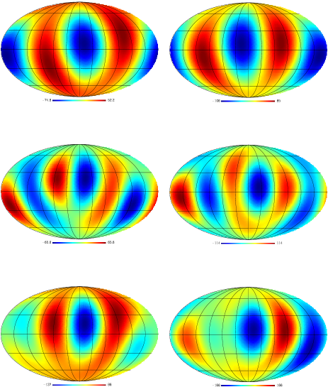
Figure 5: The left (right) panels are the quadrupole $\ell=2$, the octopole $\ell=3$ and their sum $\ell=2+3$ corresponding to the MC CMB map that produces the sigma-map-MC plotted in the middle (bottom) panel of figure 3.

A important part of our analyses are the robustness tests. To assert the robustness of our results when using a different set of parameters in the sigma-map method, we investigated the effect of changing $\gamma_{0},\,N_{\mbox{\footnotesize bins}},\,N_{\mbox{\footnotesize caps}}$, and $N_{\mbox{\footnotesize side}}$ of the CMB map in analysis, in the computation of the sigma-maps. For this we performed several sigma-map calculations using spherical caps of $\gamma_{0}=45^{\circ},\,60^{\circ}$ of aperture, $N_{\mbox{\footnotesize bins}}=45,\,60,\,90$, and $N_{\mbox{\footnotesize caps}}=768,\,3\,072$, resulting in minor differences in all these cases. Additionally, we also examine the influence of the angular resolution of the CMB maps by computing the sigma-maps considering different pixelisation parameters of the CMB maps, namely $N_{\mbox{\footnotesize side}}=16$ and $32$. In particular, the sigma-maps showed in figure 2, plotted in galactic coordinates, and their corresponding angular power spectra analyses in figure 1, were calculated using $\gamma_{0}=45^{\circ}$, $N_{\mbox{\footnotesize bins}}=45$, $N_{\mbox{\footnotesize caps}}=768$, and $N_{\mbox{\footnotesize side}}=32$. Summarizing, our robustness tests show that using a set of parameters within a certain range of values, we obtain results that are fully consistent with those showed in figure 4.

5 Conclusions

We investigated a plausible primordial scenario where a homogeneous magnetic field acting on the photon-baryon fluid at the recombination era, introduces a preferred direction that establish a statistical isotropy breaking. This setting offers a possible explanation for those anomalies found in WMAP data that seems to be associated to a preferred axis in the space, like the hemispherical NS-asymmetry and the planarity of some CMB low-order multipoles (where such a plane is perpendicular to that axis). It is found that this magnetic field induces correlations between the CMB multipoles, manifested through non-diagonal terms in the multipole correlation matrix (see eqs. (7)–(2)). Accordingly, we have simulated five sets of CMB skies considering an equal number of strengths $B_{0}$ of the magnetic field. These MC CMB maps, with multipoles in the range $\ell=2-10$, are used to investigate their large-angle correlations using our sigma-map method. With these data sets we performed a quantitative analysis of their large-angle signatures and perform a comparison with similar features computed from WMAP maps. For this, we consider a set of full-sky cleaned CMB maps, obtained from five-year and three-year WMAP data releases, namely the ILC-5yr, KCN-5yr, ILC-3yr, OT-3yr, and PPG-3yr maps, which were differently processed in order to account for foregrounds and systematic errors.

Our results can be summarized as follows. First, our analyses corroborate that an uneven hemispherical distribution in the power of the large-angular correlations, best known as NS-asymmetry phenomenon, is present in all these WMAP maps at more than 95% CL as compared with statistically isotropic CMB maps produced according to the $\Lambda$CDM cosmological model (i.e., $B_{0}=0$). Second, we found that this hemispherical asymmetry phenomenon, is such that higher is the value of the field strenght $B_{0}$, greater is the probability that such asymmetry be present in the MC CMB maps, and be revealed with a high dipole value $S_{1}^{\mbox{\sc mc}}$ in its corresponding sigma-map-MC. In other words, our results show that the correlations introduced by a magnetic field mechanism in low-order CMB multipoles, for a sufficiently intense field, reproduce the NS-asymmetry present in WMAP data as a common phenomena and not as an anomalous one. Third, as expected, the MC CMB maps with $B_{0}\neq 0$ exhibit the planarity effect in their low-order multipoles (see, for illustration, figure 5) as quantified in the Table 1, where the $\ell$-multipole power is concentrated in the $m=\pm\ell$ modes, and as evidenced by the intense red spots representative of strong angular correlations appearing in the equatorial region of the sigma-maps-MC (see, for illustration, figure 2). Fourth, as shown in the Table 1, we found a significant correlation between the NS-asymmetry and quadrupole-octopole (planarity and) alignment phenomena. For completeness, we have also verified that our results are robust under different sets of parameters, as mentioned in the previous section, involved in the sigma-map method calculations.

The large angular scales CMB anomalies challenge the statistical isotropy expected in the $\Lambda$CDM concordance model. Our results suggests that perhaps some of them could be suitable explained by just one physical phenomenon. As a matter of fact, there are several attempts to find the origin of large-angle CMB anomalies, but further investigations are needed to fully comprehend if they have one or more causes. In this sense, statistically anisotropic models explaining several anomalies with a minimum set of hipothesis should be explored.

We believe that our results shall motivate the study of other statistically anisotropic scenarios, in particular, those where correlations between CMB anomalies appear. The magnetic field scenario analysed here is just the simplest one, and considering more realistic fields new effects could be present on the CMB temperature and polarization data (see, e.g., Giovannini 2006, 2007; Giovannini & Kunze 2007; Kahniashvili & Ratra 2005; Subramanian, Seshadri & Barrow 2003; Kosowsky & Loeb 1996; Seshadri & Subramanian 2001, and references therein). In the same form, as well, possible relationships between these new effects and statistically anisotropic phenomena found in WMAP data could be established, all this deserving a better investigation.

References

- Abramo et al. (2006) Abramo L. R., Bernui A., Ferreira I. S., Villela T., Wuensche C. A., 2006, Phys. Rev. D, 74, 063506
- Abramo, Sodré & Wuensche (2006) Abramo L. R., Sodré Jr. L., Wuensche C. A., 2006, Phys. Rev. D, 74, 083515
- Ackerman, Carrol & Wise (2007) Ackerman L., Carroll S. M., Wise M. B., 2007, Phys Rev D, 75, 083502
- Adams et al. (1996) Adams J., Danielsson U. H., Grasso D., Rubinstein H., 1996, Phys. Lett. B, 253, 388
- Aurich, Lustin & Steiner (2005) Aurich R., Lustig S., Steiner F., 2005, Class. Quantum Grav., 22, 3443
- Barrow, Ferreira & Silk (1997) Barrow J. D., Ferreira P. G., Silk J., 1997, Phys. Rev. Lett., 78, 3610
- Baym, Bodeker & McLerran (1996) Baym G., Bodeker D., McLerran , 1996, Phys. Rev. D, 53, 662
- Bennett et al. (2003a) Bennett C. L. et al., 2003a, ApJS, 148, 1
- Bennett et al. (2003b) Bennett C. L. et al., 2003b, ApJS, 148, 97
- Bernui et al. (2006) Bernui A., Villela T., Wuensche C. A., Leonardi R., Ferreira I., 2006, A&A, 454, 409
- Bernui, Tsallis & Villela (2006) Bernui A., Tsallis C., Villela T., 2006, Phys. Lett. A, 356, 426
- Bernui, Tsallis & Villela (2007) Bernui A., Tsallis C., Villela T., 2007, Europhys. Lett., 78, 19001
- Bernui et al. (2007) Bernui A., Mota B., Rebouças M. J., Tavakol R., 2007, A&A, 464, 479
- Bielewicz, Górski & Banday (2004) Bielewicz P., Górski K. M., Banday A. J., 2004, MNRAS, 355, 1283
- Bielewicz et al. (2005) Bielewicz, P., Eriksen, H. K. Banday, A. J., Górski K. M., Lilje, P. B., 2005, ApJ, 635, 750
- Bunn et al. (2007) Bunn E. F., 2007, Phys. Rev. D, 75, 083517
- Clarke, Kroenberg & Boehringer (2001) Clarke T. E., Kronberg P. P., Boehringer H., 2001, ApJ, 547, L111
- Copi, Huterer & Starkman (2004) Copi C. J., Huterer D., Starkman G. D., 2004, Phys. Rev. D, 70, 043515
- Copi et al. (2007) Copi C. J., Huterer D., Schwarz D. J., Starkman G. D., 2007, Phys. Rev. D, 75, 023507
- Copi et al. (2006) Copi C. J., Huterer D., Schwarz D. J., Starkman G. D., MNRAS, 367, 79
- Cresswell et al. (2006) Cresswell J. G., Liddle A. R., Mukherjee P., Riazuelo A., 2006, Phys. Rev. D, 73, 041302
- Cruz et al. (2005) Cruz M., Martínez-González E., Vielva P., Cayón L., 2005, MNRAS, 356, 29
- Cruz et al. (2006) Cruz M., Tucci M., Martínez-González E., Vielva P. , 2006, MNRAS, 369, 57
- Cruz et al. (2007) Cruz M., Martínez-González E., Vielva P., Cayón L., 2007, ApJ, 655, 11
- Chen et al. (2004) Chen G., Mukherjee P., Kahniashvili T., Ratra B., Wang Y., 2004, ApJ, 611, 655
- Cheng & Olinto (1994) Cheng B., Olinto A. V., 1994, Phys. Rev. D, 50, 2421
- Chiang et al. (2003) Chiang L.-Y., Naselsky P. D., Verkhodanov O. V., Way M. J., 2003, ApJ, 590, L65
- Chiang et al. (2007) Chiang L.-Y., Coles P., Naselsky P. D., Olesen P., 2007, JCAP, 1, 21
- Demiański & Doroshkevich (2007) Demiański M., Doroshkevich A. G., 2007, Phys. Rev. D, 75, 123517
- de Oliveira-Costa et al. (2004) de Oliveira-Costa A., Tegmark M., Zaldarriaga M., Hamilton A., 2004, Phys. Rev. D, 69, 063516
- de Oliveira-Costa & Tegmark (2006) de Oliveira-Costa A., Tegmark M., 2006, Phys. Rev. D, 74, 023005
- Donoghue & Donoghue (2005) Donoghue E. P., Donoghue J. F., 2005, Phys. Rev. D, 71, 043002
- Dunkley et al. (2008) Dunkley J. et al., 2008, preprint (arXiv:0803.0586 [astro-ph])
- Durrer, Kahniashvili & Yates (1998) Durrer R., Kahniashvili T., Yates A., 1998, Phys. Rev. D, 58, 123004
- Dvorkin, Peiris & Hu (2007) Dvorkin C., Peiris H. V., Hu W., 2007, preprint (arXiv:0711.2321 [astro-ph])
- Eriksen et al. (2004a) Eriksen H. K., Hansen F. K., Banday A. J., Górski K. M., Lilje P. B., 2004, ApJ, 605, 14; Erratum, 2004, ApJ, 609, 1198
- Eriksen et al. (2004b) Eriksen H. K., Banday A. J., Górski K. M., Lilje P. B., 2004, ApJ, 612, 633
- Eriksen et al. (2005) Eriksen H. K., Banday A. J., Górski K. M., Lilje P. B., 2005, ApJ, 622, 58
- Eriksen et al. (2007) Eriksen H. K., Banday A. J., Górski K. M., Hansen F. K., Lilje P. B., 2007, ApJ, 660, L81
- Giovannini (2006) Giovannini M., 2006, Phys. Rev. D, 74, 06302
- Giovannini (2007) Giovannini M., 2007, Phys. Rev. D, 76, 103508
- Giovannini & Kunze (2007) Giovannini M., Kunze K. E., 2007, preprint (arXiv:0712.3483 [astro-ph])
- Gold et al. (2008) Gold B. et al., 2008, preprint (arXiv:0803.0715 [astro-ph])
- Gosh, Hajian & Souradeep (2007) Ghosh T., Hajian A., Souradeep T., 2007, Phys. Rev. D, 75, 083007
- Gordon et al. (2005) Gordon C., Hu W., Huterer D., Crawford T., 2005, Phys. Rev. D, 72 103002
- Górski et al. (2003) Górski K. M. et al., 2005, ApJ, 622, 759
- Gümrükçüoğlu, Contaldi & Peloso (2007) Gümrükçüoğlu A. E., Contaldi C. R., Peloso M., 2007, preprint (arXiv:0707.4179 [astro-ph])
- Hajian & Souradeep (2003) Hajian A., Souradeep T., 2003, ApJ, 597, L5
- Hajian, Souradeep & Cornish (2004) Hajian A., Souradeep T., Cornish T., 2004, ApJ, 618, L63
- Hajian & Souradeep (2005) Hajian A., Souradeep T., 2005, preprint (arXiv:0501001 [astro-ph])
- Hajian & Souradeep (2006) Hajian A., Souradeep T., 2006, Phys. Rev. D, 74, 123521
- Hansen, Banday & Górski (2004) Hansen F. K., Banday A. J., Górski K. M., 2004, MNRAS, 354, 641
- Hansen et al. (2004) Hansen F. K., Cabella P., Marinucci D., Vittorio N., 2004, ApJ, 607, L67
- Helling et al. (2006) Helling R. C., Schupp P., Tesileanu T., 2006, Phys. Rev. D, 74, 063004
- Hinshaw et al. (2003a) Hinshaw G. et al., 2003a, ApJS, 148, 135
- Hinshaw et al. (2003b) Hinshaw G. et al., 2003b, ApJS, 148, 63
- Hinshaw et al. (2007) Hinshaw G. et al., 2007, ApJS, 170, 288
- Hinshaw et al. (2008) Hinshaw G. et al., 2008, preprint (arXiv:0803.0732 [astro-ph])
- Huterer (2006) Huterer D., 2006, New Astron. Rev., 50, 868
- Hipólito-Ricaldi & Gomero (2005) Hipólito-Ricaldi W. S., Gomero G. I., 2005, Phys. Rev. D, 72, 103008
- Jaffe et al. (2006) Jaffe T. R., Banday A. J., Eriksen H. K., Górski K. M., Hansen F. K., 2006, A&A, 460, 393
- Jarosik et al. (2007) Jarosik N. et al., 2007, ApJS, 170, 263
- Kahniashvili & Ratra (2005) Kahniashvili T., Ratra B., 2005, Phys. Rev. D, 71, 103006
- Kahniashvili, Maravin & Kosowsky (2008) Kahniashvili T., Maravin Y., Kosowsky A., 2008, preprint (arXiv:0806.1876 [astro-ph])
- Kibble & Vilekin (1995) Kibble T. W., Vilekin A., 1995, Phys. Rev. D, 52, 679
- Kim, Naselsky & Christensen (2008) Kim J., Naselsky P., Christensen P. R., 2008, preprint (arXiv:0803.1394 [astro-ph])
- Komatsu et al. (2008) Komatsu E. et al., 2008, preprint (arXiv:0803.0547 [astro-ph])
- Kosowsky & Loeb (1996) Kosowsky A., Loeb A., 1996, ApJ, 461, 1
- Krause, Beck & Hummel (1989) Krause M., Beck R., Hummel E., 1989, A&A, 217, 17
- Kulsrud & Anderson (1992) Kulsrud R. M., Anderson S. W., 1992, ApJ, 396, 606
- Land & Magueijo (2005a) Land K., Magueijo J., 2005a, MNRAS, 357, 994
- Land & Magueijo (2005b) Land K., Magueijo J., 2005b, Phys. Rev. Lett., 95, 071301
- Land & Magueijo (2006) Land K., Magueijo J., 2006, MNRAS, 367, 1714
- Land & Magueijo (2007) Land K., Magueijo J., 2007, MNRAS, 378, 153
- López-Corredoira (2007) López-Corredoira M., 2007, preprint (arXiv:0708.4133 [astro-ph])
- McEwen et al. (2006) McEwen J. D., Hobson M. P., Lasenby A. N., Mortlock D. J., 2006, MNRAS, 371, L50
- Mukhanov (2005) Mukhanov V., 2005, Physical Foundations of Cosmology, Cambridge Univ. Press, Cambridge
- Nolta et al. (2008) Nolta M. R. et al., 2008, preprint (arXiv:0803.0593 [astro-ph])
- Naselsky & Kim (2008) Naselsky P., Kim J., 2008, preprint (arXiv:0804.3467 [astro-ph])
- Padmanabhan (1993) Padmanabhan T., Structure formation in the universe, 1993, Cambridge Univ. Press, Cambridge
- Park, Park & Gott III (2007) Park C.-G., Park C., Gott III J. R., 2007, ApJ, 660, 959
- Parker (1971) Parker E. N., 1971, ApJ, 163, 255
- Piddington (1970) Piddington J. H., 1970, Australian J. Phys, 23, 731
- Pullen & Kamionkowsi (2007) Pullen A. R., Kamionkowski M., 2007, preprint (arXiv:0709.1144 [astro-ph])
- Quashnock, Loeb & Spergel (1989) Quashnock J., Loeb A., Spergel D. N., 1989, ApJ, 344, L49
- Rakic & Schwarz (2007) Rakić A., Schwarz D. J., 2007, Phys. Rev. D, 75, 103002
- Schwarz et al. (2004) Schwarz D. J., Starkman G. D., Huterer D., Copi C. J., 2004, Phys. Rev. Lett., 93, 221301
- Seljak & Zaldarriaga (1996) Seljak U., Zaldarriaga M., 1996, www.cmbfast.org
- Seshadri & Subramanian (2001) Seshadri T. R., Subramanian K., 2001, Phys. Rev. Lett., 87, 101301
- Souradeep & Hajian (2004) Souradeep T., Hajian A., 2004, Pramana, 62, 793
- Souradeep & Hajian (2005) Souradeep T., Hajian A., 2005, preprint (arXiv:0502248 [astro-ph])
- Souradeep, Hajian & Basak (2006) Souradeep T., Hajian A., Basak S., 2006, New Astronomy Reviews, 50, 889
- Spergel et al. (2007) Spergel D. N. et al., 2007, ApJS, 170, 377
- Subramanian, Seshadri & Barrow (2003) Subramanian K., Seshadri T. R., Barrow J. D., 2003, MNRAS, 344, L31
- Tegmark, de Oliveira-Costa & Hamilton (2003) Tegmark M., de Oliveira-Costa A., Hamilton A. J. S., 2003, Phys. Rev. D, 68, 123523
- Vainshtein & Ruzmaikin (1972) Vainshtein S, I., Ruzmaikin A. A., 1972, Soviet. Astron., 15, 714
- Vainshtein & Zel’dovich (1972) Vainshtein S. I., Zel’dovich Ya. B., 1972, Sov. Phys. Usp., 15, 159
- Vachaspati (1993) Vachaspati T., 1995, Phys. Lett. B, 265, 258
- Vielva et al. (2004) Vielva P., Martínez-González E., Barreiro R. B., Sanz J. L., Cayón L., 2004, ApJ, 609, 22
- Vielva et al. (2006) Vielva P., Wiaux Y., Martínez-González E., Vandergheynst P., 2006, New Astron. Rev., 50, 880
- Vielva et al. (2007) Vielva P., Wiaux Y., Martínez-González E., Vandergheynst P., 2007, MNRAS, 381, 932
- Weeks (2004) Weeks J. R., 2004, preprint (arXiv:0412231 [astro-ph])
- Wiaux et al. (2006) Wiaux Y., Vielva P., Martínez-González E., Vandergheynst P., 2006, Phys. Rev. Lett., 96, 151303
- Wibig & Wolfendale (2005) Wibig T., Wolfendale A. W. , 2005, MNRAS, 360, 236
- Widrow (2002) Widrow M., 2002, Rev. Mod. Phys, 74, 775
- Wolfe, Lanzetta & Oren (1992) Wolfe A. M., Lanzetta K. M., Oren A. L., 1992, ApJ, 388, 17
- Xu et al. (2006) Xu Y., Kronberg P. P., Habib S., Dufton Q. W., 2006, ApJ, 637, 19