Looking Beyond Lambda with the Union Supernova Compilation

Abstract

The recent robust and homogeneous analysis of the world’s supernova distance-redshift data, together with cosmic microwave background and baryon acoustic oscillation data, provides a powerful tool for constraining cosmological models. Here we examine particular classes of scalar field, modified gravity, and phenomenological models to assess whether they are consistent with observations even when their behavior deviates from the cosmological constant $\Lambda$. Some models have tension with the data, while others survive only by approaching the cosmological constant, and a couple are statistically favored over $\Lambda{\rm CDM}$. Dark energy described by two equation of state parameters has considerable phase space to avoid $\Lambda$ and next generation data will be required to constrain such physics.

1 Introduction

A decade after the discovery of the acceleration of the cosmic expansion (Perlmutter et al., 1999; Riess et al., 1998) we still understand little about the nature of the dark energy physics responsible. Improved data continues to show consistency with Einstein’s cosmological constant $\Lambda$, and in terms of a constant equation of state, or pressure to density, ratio $w$, the best fit to the data is $w=-0.969^{+0.059}_{-0.063}({\rm stat})^{+0.063}_{-0.066}({\rm sys})$, where $\Lambda$ has $w=-1$ (Kowalski et al., 2008). However, the magnitude of $\Lambda$ required and the coincidence for it becoming dominant so close to the present remain unexplained, and an abundance of motivated or unmotivated alternative models fills the literature. Using the latest, most robust data available we examine the extent to which data really have settled on the cosmological constant.

The vast array of models proposed for dark energy makes comparison of every model in the literature to the data a Sisyphean task. Here we select some dozen models with properties such as well defined physical variables, simplicity, or features of particular physical interest. These embody a diversity of physics, including scalar fields, phase transitions, modified gravity, symmetries, and geometric relations. While far from exhaustive, they provide roadmarks for how well we can say that current data have zoomed in on $\Lambda$ as the solution.

For such comparisons it is critical to employ robust data clearly interpretable within these “beyond $\Lambda$” cosmologies. Geometric probes from the Type Ia supernovae (SN) distance-redshift relation, cosmic microwave background (CMB) acoustic peak scale shift parameter, and baryon acoustic oscillations (BAO) angular scale serve this essential role. Equally important is confidence in the error estimates, incorporating systematics as well as statistical uncertainties. This has been studied in detail in the recent unified analysis of the world’s published heterogeneous SN data sets – the Union08 compilation (Kowalski et al., 2008).

This SN compilation includes both the large data samples from the SNLS and ESSENCE survey, the compiled high redshift SNe observed with the Hubble Space Telescope, a new sample of nearby SNe, as well as several other, small data sets. All SNe have been analyzed in a uniform manner and have passed a number of quality criteria (such as having data available in two bands to measure a color, and sufficient lightcurve points to make a meaningful fit). The samples have been carefully tested for inconsistencies under a blinded protocol before combining them into a single final data set comprising 307 SNe, the basis for this analysis. In this work the SNe data will be combined with the constraints obtained from the baryon acoustic oscillation scale (Eisenstein et al., 2005) and from the five year data release of WMAP and ground based CMB measurements (Komatsu et al., 2008).

In Section 2 we describe the general method for cosmological parameter estimation and present a summary table of the various models considered and the $\chi^{2}$ statistics of the fit. Sections 3–12 then briefly describe the dark energy models, their parameters, and show the likelihood contours. The concluding discussion occurs in Section 13.

2 Constraining Models

Achieving informative constraints on the nature of dark energy requires restricting the degrees of freedom of the theory and the resulting degeneracies in the cosmological model being tested. One degree of freedom entering the model is the present matter density $\Omega_{m}$. For the case of the spatially flat cosmological constant $\Lambda$ model (or some of the other models considered below), this is the sole cosmological parameter determining the distances entering the supernova (SN) magnitude-redshift, baryon acoustic oscillation scale (BAO), and cosmic microwave background (CMB) shift parameter relations.

Generally, further degrees of freedom to describe the nature of the dark energy, i.e. its equation of state (EOS), or pressure to density, ratio, are needed. In a few cases the EOS is parameter free, as in the $\Lambda$ case where $w=-1$, or is determined by the matter density, as in some subcases below (such as the flat DGP braneworld gravity model of §4). One way to categorize models is by the number of independent EOS parameters, or general parameters beyond the matter density (so flat $\Lambda$ models have zero such parameters, $\Lambda$ models with curvature have one). In general, current data can deliver reasonable constraints on one parameter descriptions of dark energy.

In addition to exploring the nature of dark energy through its EOS, one might also include another parameter for the dark energy density, i.e. allow the possibility of nonzero spatial curvature. In this case individual probes then generally do a poor job constraining the model with current data, although the combined data from SN+CMB+BAO can sometimes still have leverage. Since crosschecks and testing consistency between probes is important (as particularly illustrated below in the DGP case), we consider spatial curvature only in the otherwise zero parameter cases of $\Lambda$ and DGP, and for the constant EOS dark energy model.

In the following sections we investigate various one parameter EOS models, discussing their physical motivation or lack thereof, and features of interest, and the observational constraints that can be placed upon them. In the last sections we also investigate some two parameter models of interest, with constrained physical behaviors and particular motivations. As a preview and summary of results, Table 1 lists the models, number of parameters, and goodness of fit for the present data.

The SN, CMB, and BAO data are combined by multiplying the likelihoods. Especially when testing models deviating from the cosmological constant one must be careful to account for any shift of the CMB sound horizon arising from violation of high redshift matter domination on the CMB and BAO scales; details are given in Union08. Note that some doubt exists on the use of the BAO constraints for cosmologies other than $\Lambda{\rm CDM}$, or possibly constant $w$, (Dick et al., 2006; Rydbeck et al., 2007) since $\Lambda{\rm CDM}$ is assumed in several places in the Eisenstein et al. (2005) analysis, e.g. computation of the correlation function from redshift space, nonlinear density corrections, structure formation and the matter power spectrum, and color and luminosity function evolution. Properly, a systematic uncertainty should be assigned to BAO to account for these effects; however, this requires a complex analysis from the original data and we show only the statistical error. At the current level of precision, simplified estimates show this does not strongly affect the results, but such systematics will need to be treated for future BAO data. All figures use the likelihood maximized over all relevant parameters besides those plotted, and contours are at the 68.3%, 95.4%, and 99.7% confidence level.

Model	Motivation	Parameters	$\chi^{2}$ (stat)		$\chi^{2}$ (sys)
$\Lambda$CDM (flat)	gravity, zeropoint	$\Omega_{m}$	313.	1	309.	9
			$\Delta\chi^{2}$ (stat)		$\Delta\chi^{2}$ (sys)
$\Lambda$CDM	gravity, zeropoint	$\Omega_{m}$, $\Omega_{\Lambda}$	$-$1.	1	$-1$.	3
Constant $w$ (flat)	simple extension	$\Omega_{m}$, $w$	$-0$.	3	$-1$.	2
Constant $w$	simple extension	$\Omega_{m}$, $\Omega_{k},w$	$-$1.	1	$-1$.	6
Braneworld	consistent gravity	$\Omega_{m}$, $\Omega_{k}$	15.	0	2.	7
Doomsday	simple extension	$\Omega_{m}$, $t_{\rm doom}$	$-$0.	1	$-0$.	7
Mirage	CMB distance	$\Omega_{m}$, $w_{0}$	$-$0.	2	$-0$.	1
Vacuum Metamorphosis	induced gravity	$\Omega_{m}$, $\Omega_{\star}$	0.	0	0.	0
Geometric DE ${\rm R_{low}}$	kinematics	$r_{0},r_{1}$ $(\Omega_{m},w_{0})$	0.	1	$-1$.	1
Geometric DE ${\rm R_{high}}$	matter era deviation	$\Omega_{m}$, $w_{\infty}$, $\beta$	$-$1.	9	$-2$.	2
PNGB	naturalness	$\Omega_{m}$, $w_{0}$, $f$	$-0$.	1	$-0$.	7
Algebraic Thawing	generic evolution	$\Omega_{m}$, $w_{0}$, $p$	$-1$.	6	$-2$.	3
Early DE	fine tuning problem	$\Omega_{m}$, $w_{0}$, $\Omega_{e}$	$-0$.	3	$-1$.	2
Growing $\nu$-mass	coincidence problem	$\Omega_{m}$, $\Omega_{e}$, $m_{\nu}^{0}$	$-0$.	6	$-1$.	6

Table 1: “Beyond $\Lambda$” dark energy models considered in this paper, together with $\Lambda$CDM models. Models are listed in the order of discussion, and the cosmological fitting parameters shown. The $\chi^{2}$ of the matter plus cosmological constant case is given, and all other models list the $\Delta\chi^{2}$ from that model. The values refer to the best fit to the joint data of SN+CMB+BAO; in the last column the SN systematics as analyzed in Union08 are included.

It is particularly important to note the treatment of systematic errors, included only for SN. We employ the prescription of Union08 for propagation of systematic errors. This introduces a new distance modulus $\mu^{\rm sys}=\mu+\Delta M_{i}+\Delta M$, which is simply the usual distance modulus $\mu=5\log(H_{0}d_{L}(z))$, where $d_{L}(z)$ is the luminosity distance and $H_{0}$ the Hubble constant, shifted by a sample dependent magnitude offset $\Delta M_{i}$ and a single sample independent magnitude offset $\Delta M$ added only for the higher redshift SNe ($z>0.2$). The magnitude offsets $\Delta M_{i}$ reflect possible heterogeneity among the SNe samples while the $\Delta M$ step from SNe at $z<0.2$ to $z>0.2$ allows a possible common systematic error in the comparison of low vs. high redshift SNe. Treating $\Delta M_{i}$ and $\Delta M$ as additional fit parameters, one defines $\chi_{\rm sys}^{2}=\chi^{2}+\sum_{i}(\Delta M_{i}/\sigma_{M_{i}})^{2}+(\Delta M/\sigma_{M})^{2}$ to absorb the uncertainty in the nuisance parameters, $\sigma_{M_{i}}$ and $\sigma_{M}$, and obtain constraints on the desired physical fit parameters that include systematic errors. This procedure of incorporating systematic errors provides robust quantification of whether or not a model is in conflict with the data and is essential for accurate physical interpretation. See Union08 for further, detailed discussion of robust treatment of systematics within the current world heterogeneous SN data.

3 Constant Equation of State

Models with constant equation of state $w$ within 20%, say, of the cosmological constant value $w=-1$, but not equal to $-1$, do not have much physical motivation. To achieve a constant equation of state requires fine tuning of the kinetic and potential energies of a scalar field throughout its evolution. It is not clear that a constant $w\neq-1$ is a good approximation to any reasonable dynamical scalar field, where $w$ varies, and certainly does not capture the key physics. However, since current data cannot discern EOS variation on timescales less than or of order the Hubble time, traditionally one phrases constraints in terms of a constant $w$. We reproduce this model from Union08 to serve as a point of comparison. Also see Union08 for models using the standard time varying EOS $w(a)=w_{0}+w_{a}(1-a)$, where $a=1/(1+z)$ is the scale factor, and models with $w(z)$ given in redshift bins.

In the constant $w$ case the Hubble expansion parameter $H=\dot{a}/a$ is given by

$$H^{2}(z)/H_{0}^{2}=\Omega_{m}(1+z)^{3}+\Omega_{w}(1+z)^{3(1+w)}+\Omega_{k}(1+z)^{2},$$ (1)

where $\Omega_{m}$ is the present matter density, $\Omega_{w}$ the present dark energy density, and $\Omega_{k}=1-\Omega_{m}-\Omega_{w}$ the effective energy density for spatial curvature.

Figure 1 shows the confidence contours in the $w$-$\Omega_{m}$ plane both without and with (minimized in the likelihood fit) spatial curvature. Note that allowing for spatial curvature does not strongly degrade the constraints. This is due to the strong complementarity of SN, CMB, and BAO data, combined with the restriction to a constant $w$ model. As shown in Union08, the constraint on curvature in this model is $\Omega_{k}=-0.010\pm 0.012$. See Union08 for more plots showing the individual probe constraints.

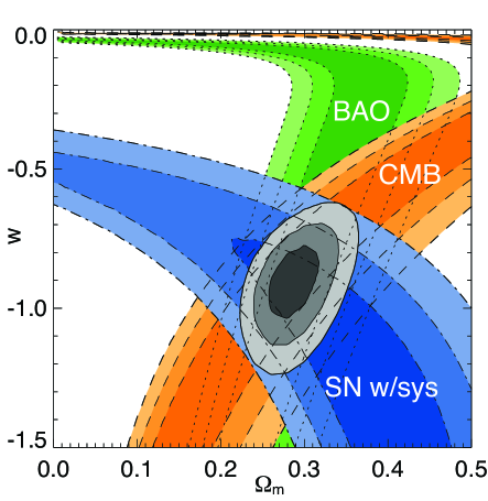
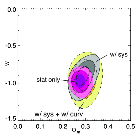
Figure 1: 68.3%, 95.4%, and 99.7% confidence level contours on a constant EOS $w$ and the matter density $\Omega_{m}$ for the individual and combined data sets. The left panel shows individual and combined probes in the flat universe case; the right panel repeats the combined systematics contour, and also compares to the statistical only contour, and to the systematics contour when simultaneously fitting for spatial curvature.

4 Braneworld Gravity

Rather than from a new physical energy density, cosmic acceleration could be due to a modification of the Friedmann expansion equations arising from an extension of gravitational theory. In braneworld cosmology (Dvali et al., 2000; Deffayet et al., 2002), the acceleration is caused by a weakening of gravity over distances near the Hubble scale due to leaking into an extra dimensional bulk from our four dimensional brane. Thus a physical dark energy is replaced by an infrared modification of gravity. For DGP braneworld gravity, the Hubble expansion is given by

$$H^{2}/H_{0}^{2} = \left(\sqrt{\Omega_{m}(1+z)^{3}+\Omega_{\rm bw}}+\sqrt{\Omega_{\rm bw}}\right)^{2}+\Omega_{k}(1+z)^{2}$$ (2)

$$\rightarrow \Omega_{m}(1+z)^{3}+2\Omega_{\rm bw}+2\sqrt{\Omega_{\rm bw}}\sqrt{\Omega_{m}(1+z)^{3}+\Omega_{\rm bw}},\qquad{\rm(flat)}\,.$$ (3)

Here the present effective braneworld energy density is

$$\Omega_{\rm bw} = \frac{(1-\Omega_{m}-\Omega_{k})^{2}}{4(1-\Omega_{k})}$$ (4)

$$\rightarrow \frac{(1-\Omega_{m})^{2}}{4},\qquad{\rm(flat)}\,,$$ (5)

and is related to the five dimensional crossover scale $r_{c}=M_{\rm Pl}^{2}/(2M_{5}^{3})$ by $\Omega_{\rm bw}=1/(4H_{0}^{2}r_{c}^{2})$. Note that the only cosmological parameters for this model are $\Omega_{m}$ and $\Omega_{k}$ (or $\Omega_{\rm bw}$), so it has the same number of parameters as $\Lambda{\rm CDM}$.

The effective dark energy equation of state is given by the simple expression

$$w(z)=-\frac{1-\Omega_{k}(z)}{1+\Omega_{m}(z)-\Omega_{k}(z)},$$ (6)

where $\Omega_{m}(z)=\Omega_{m}(1+z)^{3}/(H^{2}/H_{0}^{2})$ and $\Omega_{k}(z)=\Omega_{k}(1+z)^{2}/(H^{2}/H_{0}^{2})$. Thus the dark energy equation of state at present, $w_{0}$, is determined by $\Omega_{m}$ and $\Omega_{k}$; while time varying, it is not an independent parameter. So rather than plotting $w_{0}$ vs. $\Omega_{m}$ or showing constraints on the somewhat nonintuitive parameters $r_{c}$ or $\Omega_{\rm bw}$ (but see the clear discussion and plots in Davis et al. (2007); Rydbeck et al. (2007), though without systematics), Figure 2 illustrates the confidence contours in the $\Omega_{k}$-$\Omega_{m}$ plane. This makes it particularly easy to see how deviations from flatness pull the value of the matter density. In this and following figures, dotted contours show the BAO constraints, dashed for CMB constraints, dot-dashed for SN with systematics, and solid contours give the joint constraints.

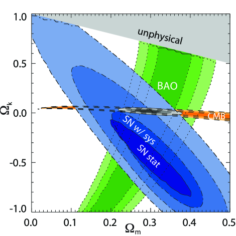
Figure 2: The extradimensional DGP braneworld gravity model does not achieve an acceptable fit to the combined data, even allowing for a spatial curvature parameter. The joint best fit is in fact a nearly flat model, but with poor goodness of fit: $\Delta\chi^{2}=2.7$ relative to the $\Lambda{\rm CDM}$ case; also shown is the statistical error only SN contour, which gives a joint $\Delta\chi^{2}=15$ relative to $\Lambda{\rm CDM}$.

For a flat universe, in order for $w$ to approach $-1$ the matter density is forced to small values. Alternately, pushing the curvature density $\Omega_{k}$ negative, i.e. introducing a positive spatial curvature $k$, allows $w\approx-1$ with higher matter density. For a given $w_{0}$, the amount of curvature needed can be derived from Eq. (6) to be approximately $\Delta\Omega_{k}\approx-\Delta\Omega_{m}/\Omega_{m}$, so to move a flat, $\Omega_{m}=0.2$ universe to $\Omega_{m}=0.3$ requires $\Omega_{k}=-0.5$, in agreement with the SN contour (being most sensitive to $w_{0}$) of Figure 2.

Note that the curvature density cannot exceed $1-\Omega_{m}$, corresponding to an infinite crossover scale $r_{c}$, so the likelihood contours are cut off at this line and the region beyond is unphysical. However, this does not affect the joint contours. The BAO data contours do extend to the limit $\Omega_{k}=1-\Omega_{m}$; here $\Omega_{\rm bw}=0$, equivalent to the simple OCDM open, nonaccelerating universe.

Most importantly, the three probes do not reach concordance on a given cosmological model. The areas of intersection of any pair are distinct from other pairs, indicating that the full data disfavors the braneworld model, even with curvature. This is further quantified by the poor goodness of fit to the data, with $\Delta\chi^{2}=2.7$ relative to the flat $\Lambda{\rm CDM}$ model possessing one fewer parameter, or $\Delta\chi^{2}=4.0$ relative to $\Lambda{\rm CDM}$ allowing curvature. This indicates the crucial importance of crosschecking probes. Moreover, if we had used only the statistical estimates of uncertainties (see the “SN stat” 68% cl contour of Fig. 2), we would have found that $\Delta\chi^{2}=15$ rather than 2.7, and possibly drawn exaggerated physical conclusions – considering the DGP model 2000 times less likely than it really is, as an illustration. Inclusion of systematics is essential for robust interpretation of results.

5 Doomsday Model

Perhaps the simplest generalization of the cosmological constant is the linear potential model, pioneered by Linde (1986) and discussed recently by Weinberg (2008), motivated from high energy physics. Interestingly, while this gives a current accelerating epoch, in the future the potential becomes negative and not only deceleration of the expansion but collapse of the universe ensues. Hence the name of doomsday model.

The potential has two parameters: the amplitude and slope. The amplitude $V_{0}$ essentially gives the dark energy density, which is fixed by $\Omega_{m}$ in a flat universe. (For the remainder of the paper we assume a flat universe, for the reasons discussed in §2.) The slope $V^{\prime}=dV/d\phi$ can be translated into the present equation of state value $w_{0}$. Thus this is a one parameter model in our categorization. See Kallosh et al. (2003) for discussion of the cosmological properties of the linear potential, Linde (1986) for a view of it as a perturbation about zero cosmological constant, and Dimopoulos (2003) for links to the large kinetic term approach in particle physics. More recently, this has been considered as a textbook case by Weinberg (2008), so we will examine this model in some detail. Such dark energy is an example of a thawing scalar field (Caldwell & Linder, 2005), starting with $w(z\gg 1)=-1$ and slowly rolling to attain less negative values of $w$; that is, it departs from $\Lambda$. If it has not evolved too far from $-1$ then its behavior is well described by $w_{a}\approx-1.5(1+w_{0})$ where $w(a)=w_{0}+w_{a}(1-a)$. However we solve the scalar field equation of motion exactly for all results quoted here.

As the scalar field rolls to small values of the potential the expansion stops accelerating, and when it reaches $V=0$ then $w=1$. However it crosses through zero to negative values of the potential, further increasing $w$, and eventually the dark energy density itself crosses through zero, causing $w$ to go to positive and then negative infinity. Thereafter the negative dark energy density, acting now as an attractive gravitational force, causes not only deceleration but forces the universe to start contracting. The rapid collapse of the universe ends in a Big Crunch, or cosmic doomsday in a finite time.

In the notation used in Weinberg (2008), $V(\phi)=V_{0}+(\phi-\phi_{0})\,V^{\prime}_{0}$, with $V_{0}$ the potential energy during the initial frozen state (during high Hubble drag at high redshift) and $V^{\prime}_{0}$ is the constant potential slope. Figure 3 shows the constraints in this high energy physics plane $V_{0}$-$V^{\prime}_{0}$. Note the tight constraints on the initial potential energy $V_{0}$, given in units of the present critical density. The cosmological constant corresponds to the limit of $V^{\prime}_{0}=0$, but the slope must always be less than or of order $10^{-120}$ in Planck units, i.e. unity when shown in terms of the present energy density, to match the data.

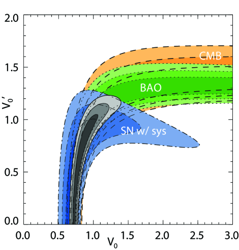
Figure 3: Constraints on the linear potential model in terms of the high energy physics quantities of the primordial amplitude and slope of the potential. Note there is less complementarity between some of the probes than for the constant $w$ model. Fig. 4 translates these constraints into ones on the cosmological parameters.

We can also translate these high energy physics parameters into the recent universe quantities of the matter density $\Omega_{m}$ and the present equation of state $w_{0}$. Moreover, this is directly related to the doomsday time $t_{\rm doom}$, or future time until collapse. A useful approximation (though we employ the exact solution) between $t_{\rm doom}$, $w_{0}$, and the approximate time variation $w_{a}=-1.5(1+w_{0})$ is

$$t_{\rm doom}\approx 0.5H_{0}^{-1}(1+w_{0})^{-0.8}\approx 0.6H_{0}^{-1}(-w_{a})^{-0.8}.$$ (7)

Figure 4 shows the likelihood contours in the $t_{\rm doom}$-$\Omega_{m}$ and $w_{0}$-$\Omega_{m}$ planes. The 95% confidence limit on $t_{\rm doom}$ from present observations is $1.24\,H_{0}^{-1}$, i.e. we are 95% likely to have at least 17 billion more years before doomsday!

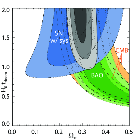
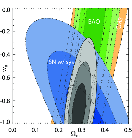
Figure 4: The future expansion history in the linear potential model has a collapse, or cosmic doomsday, at a finite time in the future. The left panel shows the confidence contours for the time remaining until collapse; the likelihood contours extend to infinity, with $t_{\rm doom}=\infty$ corresponding to the $\Lambda$ model. The contours can also be viewed in the equivalent $w_{0}$-$\Omega_{m}$ plane (right panel). Current data constraints indicate cosmic doomsday will occur no sooner than $\sim$1.24 Hubble times from now at 95% confidence.

6 Mirage Model

Given their limited sensitivity to the dynamics of dark energy, current data can appear to see a cosmological constant even in the presence of time variation. This is called the “mirage of $\Lambda$”, and we consider mirage models, with a form motivated by the observations as discussed below, specifically to test whether the concordance cosmology truly narrows in on the cosmological constant as the dark energy.

Since cosmological distances involve an integral over the energy density of components, which in turn are integrals over the equation of state as a function of redshift, there exists a chain of dependences between these quantities. Fixing a distance, such as $d_{\rm lss}$ to the CMB last scattering surface, can generally lead to an “attractor” behavior in the equation of state to a common averaged value or the value at a particular redshift. Specifically, Linder (2007) pointed out that if CMB data for $d_{\rm lss}$ is well fit by the $\Lambda{\rm CDM}$ model then this forces $w(z\approx 0.4)\approx-1$ for quite general monotonic EOS. So even dark energy models with substantial time variation could thus appear to behave like the cosmological constant at $z\approx 0.4$, near the pivot redshift of current data.

Since current experiments insensitive to time variation inherently interpret the data in terms of a constant $w$ given by the EOS value at the pivot redshift, this in turn thus leads to the “mirage of $\Lambda$”: thinking that $w=-1$ everywhere, despite models very different from $\Lambda$ being good fits. See §5.2 of Linder (2008b) for further discussion. (Also note that attempting to constrain the EOS by combining the CMB $d_{\rm lss}$ with a precision determination of the Hubble constant $H_{0}$ only tightens the uncertainty on the pivot equation of state value (already taken to be nearly $-1$) and so similarly does not reveal the true nature of dark energy.)

We test this with a family of “mirage” models motivated by the reduced distance to CMB last scattering $d_{\rm lss}$. These correspond to the one parameter subset of the two parameter EOS model $w(a)=w_{0}+w_{a}(1-a)$ with $w_{a}$ determined by $w_{a}=-3.63(1+w_{0})$. They are not exactly equivalent to imposing a CMB prior since $d_{\rm lss}$ will still change with $\Omega_{m}$; that is, they essentially test the uniqueness of the current concordance model for cosmology: $\Lambda{\rm CDM}$ with $\Omega_{m}=0.28$.

For any model well approximated by a relation $w_{a}=-A(1+w_{0})$, as this model (and the previous one) is, the Hubble parameter is given by

$$H^{2}/H_{0}^{2} = \Omega_{m}\,(1+z)^{3}+(1-\Omega_{m})\,(1+z)^{3(1+w_{0}+w_{a})}\,e^{-3w_{a}z/(1+z)}$$ (8)

$$= \Omega_{m}\,(1+z)^{3}+(1-\Omega_{m})\,(1+z)^{3(1+w_{0})(1-A)}\,e^{3A(1+w_{0})z/(1+z)}\,.$$ (9)

Figure 5 shows constraints in the $w_{0}$-$\Omega_{m}$ plane. It is important to note that $w$ is not constant in this model. A significant range of $w_{0}$ (and hence a larger range of $w_{a}$ too, roughly $+0.55$ to $-1.1$ at 68% cl) is allowed by the data, even though these models all look in an averaged sense like a cosmological constant. Thus experiments sensitive to the time variation $w_{a}$ (e.g. $\sigma(w_{a})<0.36$ to know that $w(z)$ is really, not just apparently, within 10% of $-1$) are required to determine whether the mirage is reality or not.

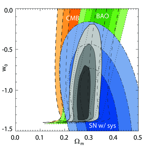
Figure 5: The mirage subclass of time varying dark energy looks like $\Lambda$ in an averaged sense. Note that CMB contours are almost vertical, indicating both that the mirage holds, preserving the $\Lambda{\rm CDM}$ distance to last scattering, and yet imposes little constraint on $w_{0}$, and hence $w_{a}$. Thus the appearance of $\Lambda$ does not actually exclude time variation. The mirage is broken when the equation of state at high redshift exceeds the matter domination value of zero; this causes the wall in the likelihood at $w_{0}=A/(1-A)\approx-1.4$.

7 Vacuum Metamorphosis

An interesting model where the cosmic acceleration is due to a change in the behavior of physical laws, rather than a new physical energy density, is the vacuum metamorphosis model (Parker & Raval, 2000; Caldwell et al., 2006). As in Sakharov’s induced gravity (Sakharov, 1968), quantum fluctuations of a massive scalar field give rise to a phase transition in gravity when the Ricci scalar curvature $R$ becomes of order the mass squared of the field, and freezes $R$ there. This model is interesting in terms of its physical origin and nearly first principles derivation, and further because it is an example of a well behaved phantom field, with $w<-1$.

The criticality condition

$$R=6(\dot{H}+2H^{2})=m^{2}$$ (10)

after the phase transition at redshift $z_{t}$ leads to a Hubble parameter

$$H^{2}/H_{0}^{2} = (1-\frac{m^{2}}{12})(1+z)^{4}+\frac{m^{2}}{12}\,,\qquad z<z_{t}\,,$$ (11)

$$H^{2}/H_{0}^{2} = \Omega_{m}(1+z)^{3}+\frac{m^{2}}{3}\frac{1-\Omega_{\star}}{4-3\Omega_{\star}}\,,\qquad z>z_{t}\,.$$ (12)

There is one parameter, $\Omega_{\star}=\Omega_{m}(z_{t})$, in addition to the present matter density $\Omega_{m}$, where $1-\Omega_{\star}$ is proportional to the cosmological constant. The variables $z_{t}$ and $m$ are given in terms of $\Omega_{m}$, $\Omega_{\star}$ by $z_{t}=(m^{2}\Omega_{\star}/[3\Omega_{m}(4-3\Omega_{\star})])^{1/3}-1$ and $m^{2}=3\Omega_{m}[(4-3\Omega_{\star})/\Omega_{\star}]^{1/4}[(4/m^{2})-(1/3)]^{-3/4}$. The original version of the model had fixed $\Omega_{\star}=1$, i.e. no cosmological constant, but if the scalar field has nonzero expectation value (which is not required for the induced gravity phase transition) then there will be a cosmological constant, and $\Omega_{\star}$ deviates from unity.

Figure 6 shows the confidence contours in the $\Omega_{\star}$-$\Omega_{m}$ plane. To consider constraints on the original vacuum metamorphosis model, without an extra cosmological constant, slice across the likelihood contours at the $\Omega_{\star}=1$ line. We see that the three probes are inconsistent with each other in this case, with disjoint contours (indeed the $\Delta\chi^{2}=28.5$ relative to flat $\Lambda{\rm CDM}$). Allowing for a cosmological constant, i.e. $\Omega_{\star}\neq 1$, brings the probes into concordance, and the best joint fit approaches the lower bound of the region $\Omega_{\star}\geq\Omega_{m}$. The condition $\Omega_{\star}=\Omega_{m}$ corresponds to the standard cosmological constant case, with $\Omega_{\Lambda}=1-\Omega_{m}$, since the phase transition then only occurs at $z_{t}=0$. Thus the data do not favor any vacuum phase transition. Although this model comprises very different physics, and allows phantom behavior, the data still are consistent with the cosmological constant.

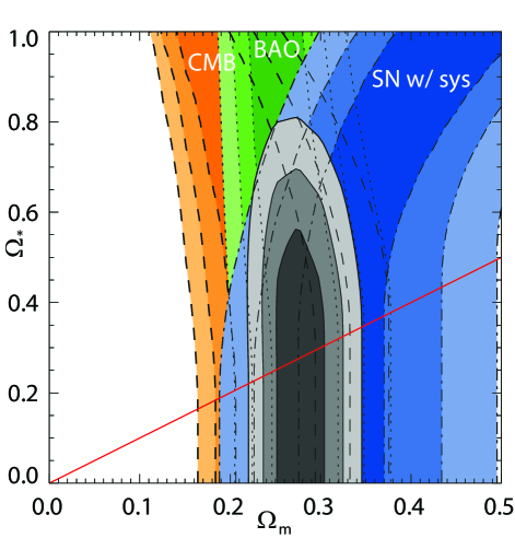
Figure 6: The vacuum metamorphosis model involves a phase transition in gravitational laws due to quantum effects. Where the quantum field inducing the gravitational deviation has no additional zeropoint energy, i.e. cosmological constant, then $\Omega_{\star}=1$, and the data gives discordant results. As the model approaches the $\Omega_{\star}=\Omega_{m}$ line of pure cosmological constant plus matter without a phase transition in the past, the data provide an increasingly good fit. (Below the line, the transition takes place further into the future, with no effect on the data likelihood.)

8 Geometric Dark Energy

According to the Equivalence Principle, acceleration is manifest in the curvature of spacetime, so it is interesting to consider geometric dark energy, the idea that the acceleration arises from some property of the spacetime geometry. One example of this involves the holographic principle of quantum field theory as applied to cosmology. This limits the number of modes available to the vacuum energy and so could have an impact on the cosmological constant problem (Bousso, 2002). The basic idea is that there is a spacelike, two dimensional surface on which all the field information is holographically encoded, and the covariant entropy bound relates the area of this surface to the maximum mode energy allowed (UV cutoff). The vacuum energy density resulting from summing over modes ends up being proportional to the area, or inverse square of the characteristic length scale. However, what is perhaps the natural surface to choose, the causal event horizon, does not lead to an energy density with accelerating properties.

Many of the attempts in the literature to overcome this have grown increasingly distant from the original concept of holography, though they often retain the name. It is important to realize that, dimensionally, any energy density, including the vacuum energy density, has $\rho\sim L^{-2}$, so merely choosing some length $L$ does not imply any connection to quantum holography. We therefore do not consider these models but turn instead to the spacetime curvature.

8.1 Ricci dark energy ${\rm R_{low}}$

A different approach involves the spacetime curvature directly, as measured through the Ricci scalar. This is similar in motivation to the vacuum metamorphosis model of §7. Here we consider it purely geometrically, with the key physical quantity being the reduced scalar spacetime curvature, in terms of the Ricci scalar and Hubble parameter, as in the model of Linder (2004),

$$\mathcal{R}\equiv\frac{R}{12H^{2}}=r_{0}+r_{1}(1-a).$$ (13)

This quantity directly involves the acceleration. Moreover, we can treat it purely kinematically, as in the last equality above, assuming no field equations or dynamics. Of course, any functional form contains an implicit dynamics (see, e.g., Linder (2008b)), but we have chosen effectively a Taylor expansion in the scale factor $a$, valid for any dynamics for small deviations $1-a$ from the present, i.e. the low redshift or low scalar curvature regime.

At high redshift, as $1-a$ is no longer small, we match it onto an asymptotic matter dominated behavior for $a<a_{t}=1-(1-4r_{0})/(4r_{1})$. Solving for the Hubble parameter,

$$H^{2}/H_{0}^{2} = a^{4(r_{0}+r_{1}-1)}\,e^{4r_{1}(1-a)},\quad a>a_{t}$$ (14)

$$H^{2}/H_{0}^{2} = \Omega_{m}\,a^{-3},\quad a<a_{t}\,.$$ (15)

The matching condition determines

$$\Omega_{m}=\left(\frac{4r_{0}+4r_{1}-1}{4r_{1}}\right)^{4r_{0}+4r_{1}-1}\,e^{1-4r_{0}},$$ (16)

so there is only one parameter independent of the matter density.

Note also that we can define an effective dark energy as that part of the Hubble parameter deviating from the usual matter behavior, with equation of state generally given by

$$w(a)=\frac{1-4\mathcal{R}}{3}\,\left[1-\Omega_{m}\,e^{-\int_{a}^{1}(da/a)(1-4\mathcal{R})}\right]^{-1}\,.$$ (17)

For the particular form of Eq. (13) we have

$$w_{0}\to\frac{1-4r_{0}}{3(1-\Omega_{m})}\,.$$ (18)

This model has one EOS parameter in addition to the matter density. We can therefore explore constraints either in the general kinematic plane $r_{0}$-$r_{1}$, or view them in the $\Omega_{m}$-$w_{0}$ plane. Figure 7 shows both.

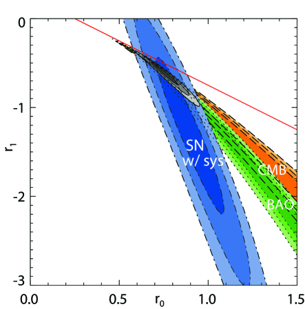
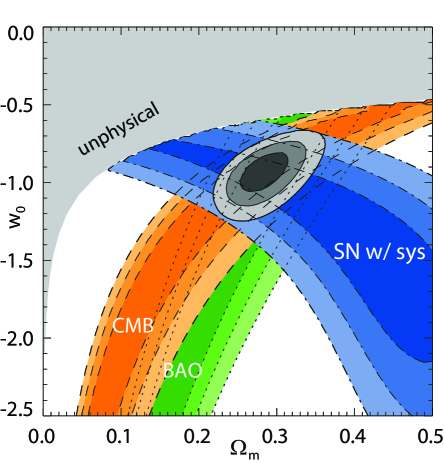
Figure 7: Geometric dark energy in the ${\rm R_{low}}$ model describes the acceleration directly through the reduced Ricci scalar, or spacetime curvature. This can be viewed in a kinematic sense, in the $r_{0}$-$r_{1}$ plane, or in a dark energy sense in the $\Omega_{m}$-$w_{0}$ plane. The data favor $w_{0}=-1$ but this is not $\Lambda$, instead representing distinct physics. For $r_{0}+r_{1}>1/4$, above the diagonal line, early matter domination is violated, and the CMB and BAO likelihoods avoid this region, as seen in the left panel; the matter density also cannot then be uniquely defined so the equivalent region is excluded from the right panel.

Good complementarity, as well as concordance, exists among the probes in the $r_{0}$-$r_{1}$ plane. One obtains an excellent fit with $(r_{0},r_{1})=(0.81,-0.72)$. The value of $\mathcal{R}$ today, $r_{0}$, approaches unity, the deSitter value. Recall that $\mathcal{R}=1/4$ corresponds to matter domination, and $\mathcal{R}=1/2$ to the division between decelerating and accelerating expansion, so this kinematic approach clearly indicates the current acceleration of the universe.

An interesting point to note is that $\Lambda{\rm CDM}$ is not a subset of this ansatz, i.e. the physics is distinct. No values of $r_{0}$ and $r_{1}$ give a $\Lambda{\rm CDM}$ cosmology. However, the Hubble diagram for the best fit agrees with that for $\Lambda{\rm CDM}$ to within 0.006 mag out to $z=2$ and 0.3% in the reduced distance to CMB last scattering. This is especially interesting as this geometric dark energy model is almost purely kinematic. The agreement appears in the $\Omega_{m}$-$w_{0}$ plane as contours tightly concentrated around $w_{0}=-1$, despite there being no actual scalar field or cosmological constant. Again we note the excellent complementarity between the individual probes, even in this very different model.

8.2 Ricci dark energy ${\rm R_{high}}$

Rather than expanding the spacetime curvature around the present value we can also consider the deviation from a high redshift matter dominated era. That is, we start with a standard early universe and ask how the data favors acceleration coming about. In this second geometric dark energy model (call it ${\rm R_{high}}$ for high redshift or large values of scalar curvature), the value of $\mathcal{R}$ evolves from $1/4$ at high redshift. From the definition of $\mathcal{R}$, it must behave asymptotically as

$$\mathcal{R}=\frac{1}{4}\,\left[1-3w_{\infty}\frac{\delta H^{2}}{H^{2}}\right]\approx\frac{1}{4}\,[1+4\alpha\,a^{-3w_{\infty}}],$$ (19)

where $\delta H^{2}=(H^{2}/H_{0}^{2})-\Omega_{m}\,(1+z)^{3}$ is the deviation from matter dominated behavior, and $w_{\infty}$ is the associated, effective equation of state at high redshift, approximated as asymptotically constant.

Next we extend this behavior to a form that takes the reduced scalar curvature to a constant in the far future (as it must if the EOS of the dominant component goes to an asymptotic value):

$$\mathcal{R}=\frac{1}{4}+\frac{\alpha\,a^{-3w_{\infty}}}{1+\beta\,a^{-3w_{\infty}}}.$$ (20)

So today $\mathcal{R}=1/4+\alpha/(1+\beta)$ and in the future $\mathcal{R}=1/4+\alpha/\beta$. By requiring the correct form for the high redshift Hubble expansion, one can relate the parameters $\alpha$ and $\beta$ by

$$\alpha=(3\beta w_{\infty}/4)[\ln\Omega_{m}/\ln(1+\beta)]\,,$$ (21)

and finally

$$H^{2}/H_{0}^{2}=\Omega_{m}\,a^{-3}\,(1+\beta a^{-3w_{\infty}})^{-\ln\Omega_{m}/\ln(1+\beta)}.$$ (22)

The ${\rm R_{high}}$ geometric dark energy model has two parameters $\beta$ and $w_{\infty}$, in addition to the matter density $\Omega_{m}$. This is the first such model we consider, and all remaining models also have two EOS parameters. Although current data cannot in general satisfactorily constrain two parameters, and so for all remaining models we do not show individual probe constraints, if the EOS phase space behavior of the model is sufficiently restrictive then reasonable joint constraints may result.

Figure 8 shows the joint likelihoods in the $\Omega_{m}$-$w_{\infty}$ and $\Omega_{m}$-$\beta$ planes, with the third parameter minimized over. We see that the data are consistent with the cosmological constant behavior $w_{\infty}=-1$ in the past (this is only a necessary, not sufficient condition for $\Lambda{\rm CDM}$), and indeed constrain the asymptotic high redshift behavior reasonably well, in particular to negative values of $w_{\infty}$. This indicates that the Ricci scalar curvature definitely prefers a nearly-standard early matter dominated era, i.e. the deviations faded away into the past. This has important implications as well for scalar-tensor theories that would modify the early expansion history; in particular, the data indicate that deviations in $\mathcal{R}$ must go approximately as $a^{3}$ (see Linder & Cahn (2007)) not as $a$ as sometimes assumed.

The parameter $\beta$ helps determine the rapidity of the Ricci scalar transition away from matter domination. This varies between $\beta=0$, giving a slow transition but one reaching a deceleration parameter $q=-\infty$ in the asymptotic future, and $\beta\gg 1$, giving a rapid deviation but with smaller magnitude. A cosmological constant behavior has $\beta\approx 3$, as discussed below.

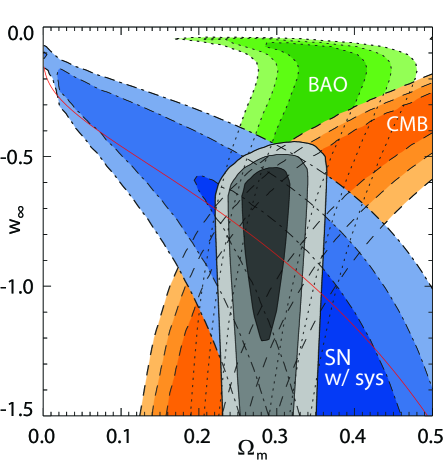
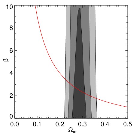
Figure 8: Geometric dark energy in the ${\rm R_{high}}$ model describes the acceleration directly through the reduced Ricci scalar curvature and deviations from early matter domination. The left panel shows the $\Omega_{m}$-$w_{\infty}$ plane, indicating the nature of the deviation ($w_{\infty}=0$ corresponds to no transition away from matter domination), and the right panel shows the $\Omega_{m}$-$\beta$ plane, indicating the rapidity and fate of the deviation. The curve in the left panel corresponds to whether the fate of the universe is de Sitter; we also show the individual probe constraints, fixing $\beta$ to the de Sitter value (not minimizing over $\beta$ as for the joint contour), to show that SN closely map the fate of the universe. In the right panel the curve is the cut through parameter space, fixing $w_{\infty}=-1$, corresponding to $\Lambda{\rm CDM}$.

Within the three dimensional parameter space, two subspaces are of special interest. One is where $w_{\infty}=-1$, a necessary condition for consistency with $\Lambda$, as mentioned. The other corresponds to a deSitter asymptotic future, defined by the line

$$\beta_{\rm deS}=\Omega_{m}^{w_{\infty}}-1.$$ (23)

Note that unlike the previous geometric model ${\rm R_{low}}$, the ${\rm R_{high}}$ model does include $\Lambda$ as the limit when both these conditions are satisfied, $w_{\infty}=-1$ and $\beta=\Omega_{m}^{-1}-1$. This relation for the $\Lambda$ limit is shown as a curve in the $\Omega_{m}$-$\beta$ plane. There is an overlap with the joint data likelihood, though one must be careful since the contours have been minimized over $w_{\infty}$.

Interestingly, we can actually use the data to test consistency with a de Sitter asymptotic future. This is shown by the curve in the $\Omega_{m}$-$w_{\infty}$ plane. We see that SN are the probe most sensitive to testing the fate of the universe, with the SN contour oriented similarly to the curve given by Eq. (23) that passes through the best fit. Thus the data are consistent with $w_{\infty}=-1$ and with a de Sitter fate separately, though some tension exists between satisfying them simultaneously. Thus, this geometric dark energy may be distinct from the cosmological constant.

9 PNGB Model

Returning to high energy physics models for dark energy, one of the key puzzles is how to prevent quantum corrections from adding a Planck energy scale cosmological constant or affecting the shape of the potential. This is referred to as the issue of technical naturalness. Pseudo-Nambu Goldstone boson (PNGB) models are technically natural, due to a shift symmetry, and so can be considered strongly physically motivated (perhaps even more so than $\Lambda$). See Frieman (1995) for an early cosmological analysis of PNGB as dark energy and more recent work by Dutta & Sorbo (2007); Abrahamse et al. (2008).

The potential for the PNGB model is

$$V(\phi)=V_{\star}\,[1+\cos(\phi/f)],$$ (24)

with $V_{\star}$ setting the magnitude, $f$ the symmetry energy scale or steepness of the potential, and $\phi_{i}$ is the initial value of the field when it thaws from the high redshift, high Hubble drag, frozen state. These three parameters determine, and can be thought of as roughly analogous to, the dark energy density, the time variation of the equation of state, and the value of the equation of state. The dynamics of this class of models is sometimes approximated by the simple form

$$w(a)=-1+(1+w_{0})a^{F},$$ (25)

with $F$ roughly inversely related to the symmetry energy scale $f$, but we employ the exact numerical solutions of the field evolution equation.

PNGB models are an example of thawing dark energy, where the field departs recently from its high redshift cosmological constant behavior, evolving toward a less negative equation of state. Since the EOS only deviates recently from $w=-1$, the precision in measuring $w_{0}$ is more important than the precision in measuring an averaged or pivot EOS value. SN data provide the tightest constraint on $w_{0}$. In the future the field oscillates around its minimum with zero potential and ceases to accelerate the expansion, acting instead like nonrelativistic matter.

Figure 9 illustrates the constraints in both the particle physics and cosmological parameters. The symmetry energy scale could provide a key clue for revealing the fundamental physics behind dark energy, and it is interesting to note that these astrophysical observations essentially probe the Planck scale. For values of $f$ below unity (the reduced Planck scale), the potential is steeper, causing greater evolution away from the cosmological constant state. However, the field may be frozen until recently and then quickly proceed down the steep slope, allowing values of $w_{0}$ far from $-1$ but looking in an average or constant $w$ sense like $\langle w\rangle\approx-1$. Small values of $\phi_{i}/f$ have the field set initially ever more finely near the top of the potential; starting from such a flat region the field rolls very little and $w$ stays near $-1$ even today. In the limit $\phi_{i}/f=0$ the field stays at the maximum, looking exactly like a cosmological constant. The two effects of the steepness and initial position mean that the cosmological parameter likelihood can accommodate both $w_{0}\approx-1$ and $w_{0}$ approaching 0 as consistent with current data. However, to agree with data and $1+w_{0}\sim 1$ requires $f\ll 1$ and fine tuning – e.g. for $f=0.1$ one must balance the field to within one part in a thousand of the top. Thus in the left panel there exists an invisibly narrow tail extending along the y-axis to $f=0$. In the right panel, we show how taking more natural values $f\gtrsim 0.5$ removes the more extreme values of $w_{0}$ caused by the unnatural fine tuning.

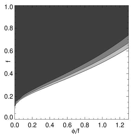
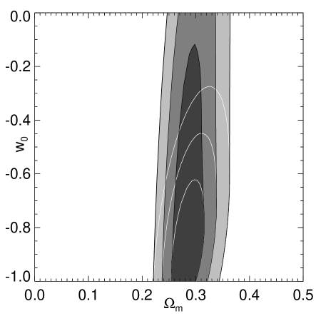
Figure 9: Left panel: PNGB model dynamics involves a competition between the steepness of the potential, given by the symmetry energy scale $f$, and the initial field position $\phi_{i}/f$. If the potential is very steep, $f\ll 1$, the field will roll so rapidly to the potential minimum that the dark energy density never becomes significant, unless $\phi_{i}/f$ is fine tuned very near zero. For natural energy scale values near the Planck scale, $f\approx 1$, a wide variety of $\phi_{i}/f$ are viable. Right panel: The field spends a long period frozen, acting as a cosmological constant before thawing and evolving to a present EOS $w_{0}$. For steep potentials with $f\ll 1$, the thawing can be rapid and result in evolution to $w_{0}$ far from $-1$, yet still be consistent with data. The solid confidence level contours in the $w_{0}$-$\Omega_{m}$ plane show PNGB results for energy scales $f\geq 0.1$, while the white outline contours consider only PNGB models with more natural energy scales $f\geq 0.5$; the latter favors models closer to the cosmological constant behavior.

10 Algebraic Thawing Model

While PNGB models involve a pseudoscalar thawing field, we can also consider scalar fields with thawing behavior. Any such fields that are neither fine tuned nor have overly steep potentials must initially depart from the cosmological constant behavior along a specific track in the EOS phase space, characterized by a form of slow roll behavior in the matter dominated era. (See Caldwell & Linder (2005); Linder (2006); Scherrer & Sen (2008); Cahn et al. (2008).) Here we adopt the algebraic thawing model of Linder (2008a), specifically designed to incorporate this physical behavior:

$$1+w = (1+w_{0})\,a^{p}\,\left(\frac{1+b}{1+ba^{-3}}\right)^{1-p/3}$$ (26)

$$H^{2}/H_{0}^{2} = \Omega_{m}\,a^{-3}+(1-\Omega_{m})\,\exp\left[\frac{3(1+w_{0})}{\alpha p}\left\{1-(1-\alpha+\alpha a^{3})^{p/3}\right\}\right],$$ (27)

where $\alpha=1/(1+b)$ and $b=0.3$ is a fixed constant not a parameter. The two parameters are $w_{0}$ and $p$ and this form fulfills the physical dynamics condition not only to leading but also next-to-leading order (Cahn et al., 2008).

The physical behavior of a minimally coupled scalar field evolving from a matter dominated era would tend to have $p\in[0,3]$. Since we want to test whether the data points to such a thawing model, we consider values of $p$ outside this range. Results are shown in Figure 10.

For $p<0$, the field has already evolved to its least negative value of $w$ and returned toward the cosmological constant. The more negative $p$ is, the less negative (closer to 0) the extreme value of $w$ is, so these models can be more tightly constrained as $p$ gets more strongly negative. As $p$ gets more positive, the field takes longer to thaw, increasing its similarity to the cosmological constant until recently, when it rapidly evolves to $w_{0}$. Such models will be very difficult to distinguish from $\Lambda$. If we restrict consideration to the physically expected range $p\in[0,3]$, this implies $w_{0}<-0.57$ at 95% confidence in these thawing models, so considerable dynamics remains allowed under current data. This estimation is consistent with the two specific thawing models already treated, the doomsday and PNGB cases.

The goodness of fit to the data is the best of all models considered here, even taking into account the number of fit parameters. This may indicate that we should be sure to include a cosmological probe sensitive to $w_{0}$ (not necessarily the pivot EOS $w_{p}$) and to recent time variation $w_{a}$, such as SN, in our quest to understand the nature of dark energy.

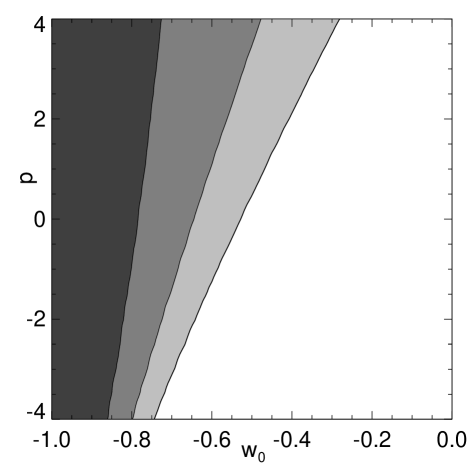
Figure 10: Algebraic thawing model incorporates the expected physical behavior of a thawing scalar field rolling slowly from a matter dominated era. Such a model is a fairly generic parametrization for this class of physics when $p\in[0,3]$, and has a strong goodness of fit.

11 Early Dark Energy

The other major class of dark energy behavior is that of freezing models, which start out dynamical and approach the cosmological constant in their evolution. The tracking subclass is interesting from the point of view again of fundamental physics motivation: they can ameliorate the fine tuning problem for the amplitude of the dark energy density by having an attractor behavior in their dynamics, drawing from a large basin of attraction in initial conditions (Zlatev et al., 1999). Such models generically can have nontrivial amounts of dark energy at high redshift; particularly interesting are scaling models, or tracers, where the dark energy has a fixed fraction of the energy density of the dominant component. These can be motivated by dilatation symmetry in particle physics and string theory (Wetterich, 1988).

As a specific model of such early dark energy we adopt that of Doran & Robbers (2006), with

$$\Omega_{\rm DE}(a)=\frac{1-\Omega_{m}-\Omega_{e}\,(1-a^{-3w_{0}})}{1-\Omega_{m}+\Omega_{m}a^{3w_{0}}}+\Omega_{e}\,(1-a^{-3w_{0}})$$ (28)

for the dark energy density as a function of scale factor $a=1/(1+z)$. Here $\Omega_{\rm DE}=1-\Omega_{m}$ is the present dark energy density, $\Omega_{e}$ is the asymptotic early dark energy density, and $w_{0}$ is the present dark energy EOS. In addition to the matter density the two parameters are $\Omega_{e}$ and $w_{0}$.

The Hubble parameter is given by $H^{2}/H_{0}^{2}=\Omega_{m}\,a^{-3}/[1-\Omega_{\rm DE}(a)]$. The standard formula for the EOS, $w=-1/(3[1-\Omega_{\rm DE}(a)])\,d\ln\Omega_{\rm DE}(a)/d\ln a$, does not particularly simplify in this model. Note that the dark energy density does not act to accelerate expansion at early times, and in fact $w\to 0$. However, although the energy density scales like matter at high redshift, it does not appreciably clump and so slows growth of matter density perturbations. We will see this effect is crucial in constraining early dark energy.

Figure 11 shows the constraints in the $\Omega_{m}$-$\Omega_{e}$ and $\Omega_{e}$-$w_{0}$ planes. Considerable early dark energy density appears to be allowed, but this is only because we used purely geometric information, i.e. distances and the acoustic peak scale. The high redshift Hubble parameter for a scaling solution is multiplied by a factor $1/\sqrt{1-\Omega_{e}}$ relative to the case without early dark energy (see Doran et al. (2007a)). This means that the sound horizon is shifted according to $s\sim\sqrt{1-\Omega_{e}}$, but a geometric degeneracy exists whereby the acoustic peak angular scale can be preserved by changing the value of the matter density $\Omega_{m}$ (see Linder & Robbers (2008) for a detailed treatment). This degeneracy is clear in the left panel.

However, as mentioned, the growth of perturbations is strongly affected by the unclustered early dark energy. This suppresses growth at early times, leading to a lower mass amplitude $\sigma_{8}$ today. To explore the influence of growth constraints, we investigate adding a growth prior of 10% to the data, i.e. we require the total linear growth (or $\sigma_{8}$) to lie within 10% of the concordance model. The innermost, white contour of the left panel of Fig. 11 shows the constraint with the growth prior. In the right panel we zoom in, and show $\Omega_{e}$ vs. $w_{0}$, seeing that the degeneracy is effectively broken. The amount of early dark energy is limited to $\Omega_{e}<0.038$ at 95% cl. Similar conclusions were found in a detailed treatment by Doran et al. (2007b).

We find a convenient fitting formula is that for an early dark energy model the total linear growth to the present is suppressed by

$$\frac{\Delta g_{0}}{g_{0}}\approx\left(\frac{\Omega_{e}}{0.01}\right)\times 5.1\%,$$ (29)

relative to a model with $\Omega_{e}=0$ but all other parameters fixed. Thus appreciable amounts of early dark energy have significant effects on matter perturbations, and we might expect nonlinear growth to be even more sensitive (e.g. see Bartelmann et al. (2006)).

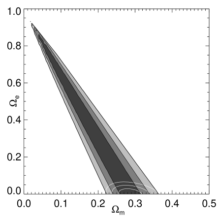
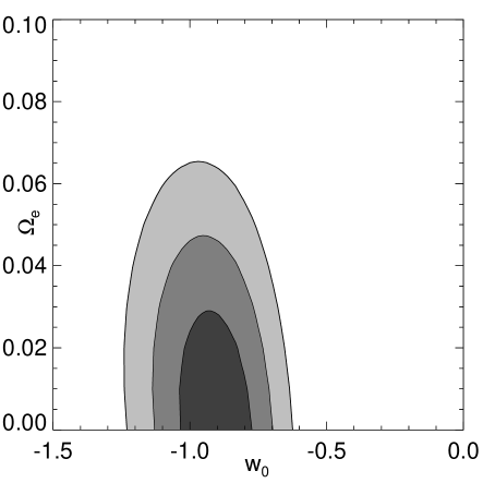
Figure 11: Early dark energy represents an example of a freezing model with interesting particle physics motivations. The left panel shows the constraints on $\Omega_{e}$ and $\Omega_{m}$ from purely geometric data, as used throughout this article. The degeneracy evident in the contours leaves the acoustic scales unchanged, but hides the shift in the sound horizon caused by early dark energy, leading to possible misinterpretation of the correct cosmological model. The degeneracy can be broken by adding growth information, here a 10% prior on total linear growth (or $\sigma_{8}$), as shown by the white outline contours. This tightly restricts the early dark energy density to contribute no more than a few percent. The right panel shows the $\Omega_{e}$-$w_{0}$ constraints including the growth prior.

12 Growing Neutrino Model

While freezing or scaling models such as the early dark energy model just considered are interesting from the physics perspective, they generically have difficulty in evolving naturally to sufficiently negative EOS by the present. The growing neutrino model of Amendola et al. (2007); Wetterich (2007) solves this by coupling the scalar field to massive neutrinos, forcing the scalar field to a near cosmological constant behavior when the neutrinos go nonrelativistic. This is an intriguing model that solves the coincidence problem through cosmological selection (the time when neutrinos become nonrelativistic) rather than tuning the Lagrangian.

The combined dark sector (cosmon scalar field plus mass-running neutrinos) energy density is

$$\Omega_{\rm ds}(a) = \frac{\Omega_{\rm ds}a^{3}+2\Omega_{\nu}(a^{3/2}-a^{3})}{1-\Omega_{\rm ds}(1-a^{3})+2\Omega_{\nu}(a^{3/2}-a^{3})},\qquad a>a_{t}$$ (30)

$$\Omega_{\rm ds}(a) = \Omega_{e},\qquad\qquad\qquad\qquad\qquad a<a_{t}\,,$$ (31)

where $\Omega_{\rm ds}=1-\Omega_{m}$ is the present dark sector energy density. The Hubble parameter can be found by $H^{2}/H_{0}^{2}=\Omega_{m}a^{-3}/[1-\Omega_{\rm ds}(a)]$ as usual. The two free dark parameters are the neutrino mass or density $\Omega_{\nu}=m_{\nu}(z=0)/(30.8h^{2}\,{\rm eV})$ and the early dark energy density $\Omega_{e}$. The transition scale factor $a_{t}$ is determined by intersection of the two behaviors given for $\Omega_{\rm ds}(a)$.

The equation of state is

$$w=-1+\frac{\Omega_{\nu}a^{-3/2}}{\Omega_{\rm ds}+2\Omega_{\nu}(a^{-3/2}-1)},\qquad a>a_{t}$$ (32)

with $w=0$ before the transition, i.e. a return to the standard early dark energy model. One can therefore translate $\Omega_{\nu}$ or $m_{\nu}(z=0)$ into $w_{0}=-1+\Omega_{\nu}/\Omega_{\rm ds}=-1+\Omega_{\nu}/(1-\Omega_{m})$.

Figure 12 shows the constraints in the $m_{\nu}(z=0)$-$\Omega_{e}$ plane. As in the previous early dark energy model, the geometric degeneracy is clear. Again, when we add growth information in the form of a 10% prior on the total linear growth (or the mass variance $\sigma_{8}$), the constraints tighten considerably, as shown in the right panel. The 95% confidence level limit on the neutrino mass from this current cosmological data is then $2.1\,(h/0.7)^{2}$ eV ($1.2$ if only statistical uncertainties are taken into account). These limits are comparable to astrophysical constraints from similar types of data applied to standard, constant mass neutrinos (Goobar et al., 2006; Tegmark et al., 2006). Note that because the neutrino mass grows due to the coupling, the value today can actually be larger than that at, say, $z\approx 3$ where Lyman alpha forest constraints apply (Seljak et al., 2006).

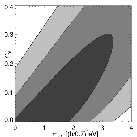
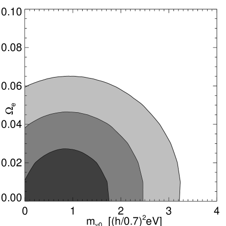
Figure 12: Growing neutrino model, coupling a dark energy scalar field to massive neutrinos, can solve the coincidence problem. The left panel shows the constraints from purely geometric data, while the right panel (note the different vertical scale) adds a 10% prior on total linear growth (also see Fig. 11). The neutrino mass today becomes tightly constrained to an interesting range, and comparison with laboratory limits could lead to evidence of varying neutrino mass.

13 Conclusion

We have considered a wide variety of dark energy physics quite different from the cosmological constant. These include a diversity of physical origins for the acceleration of the expansion: from dynamical scalar fields to dark energy that will eventually cause deceleration and collapse, to gravitational modifications arising from extra dimensions or from quantum phase transitions, to geometric or kinematic parametrization of the acceleration, to dark energy that may have influenced the early universe and that may have its magnitude set by the neutrino mass. The comparison to $\Lambda{\rm CDM}$ and constant $w$ cases covers 5 one-parameter and 5 two-parameter dark energy equation of state models. (Linder & Huterer (2005) detail how even next generation data will not generically be able to tightly constrain more than two such parameters.)

Two key results to emphasize are that current data 1) are consistent with $\Lambda$, and 2) are also consistent with a diversity of other models and theories, even when we restrict consideration to those with at least modest physical motivation or justification. As explicitly shown by the mirage model, any inclination toward declaring $\Lambda$ the answer based on consideration of a constant $w$ has an overly restricted view. The need for next generation observations with far greater accuracy, and the development of precision growth probes, such as weak gravitational lensing, is clear. All major classes of physics to explain the nature of dark energy are still in play.

However there are already quite hopeful signs of imminent progress in understanding the nature of dark energy. For example, for the braneworld model tight control of systematics would decrease the goodness of fit to $\Delta\chi^{2}=+15$, even allowing for spatial curvature, diminishing its likelihood by a factor 2000 naïvely, effectively ruling out the model. For the doomsday model, improving errors by 30% extends our “safety margin” against cosmic collapse by 10 billion years – a nonnegligible amount! Every improvement in uncertainties pushes the limits on the neutrino mass within the growing neutrino model closer toward other astrophysical constraints – plus this model essentially guarantees a deviation from $w=-1$ of $0.1\,(m_{\nu 0}/{\rm eV})$, excitingly tractable. Terrestrial neutrino oscillation bounds already provide within this model that $1+w>0.005$.

As points of interest, we note that the model with noticeably positive $\Delta\chi^{2}$ relative to $\Lambda$, and hence disfavored, is completely distinct from the cosmological constant, i.e. the braneworld model has no limit within its parameter spaces equivalent to $\Lambda$. This does not say that no such model could fit the data – the $R_{\rm low}$ model is also distinct from $\Lambda$ but fits as well as many models. Certainly many successful models under current data do look in some averaged sense like a vacuum energy but this does not necessarily point to static dark energy. Two serious motivations to continue looking for deviations are that physicists have failed for 90 years to explain the magnitude required for a cosmological constant, and that the previous known occurrence of cosmic acceleration – inflation – evidently involved a dynamical field not a cosmological constant.

To guide further exploration of the possible physics, we highlight those models which do better than $\Lambda$: the geometric dark energy and algebraic thawing approaches. One of the sole models where adding a degree of freedom is justified (albeit modestly) by the resulting reduction in $\chi^{2}$ is the ${\rm R_{high}}$ model directly studying deviations of the spacetime curvature from the matter dominated behavior. This has one more parameter than the constant $w$ EOS approach, but improves in $\chi^{2}$ by 1. In addition, it has a built-in test for the asymptotic de Sitter fate of the future expansion. We recommend that this model be considered a model of interest for future fits. The other model improving by at least one unit of $\chi^{2}$ is the algebraic thawing model, performing better than the other thawing models, with a general parametrization explicitly incorporating the physical conditions imposed by matter domination on the scalar field dynamics.

The diversity of models also illustrates some properties of the cosmological probes beyond the familiar territory of vanilla $\Lambda{\rm CDM}$. For example, for the algebraic thawing and other such evolutionary models, the premium is on precision of $w_{0}$ and $w_{a}$ much more than the averaged or pivot EOS value $w_{p}$. Not all models possess the wonderful three-fold complementarity of the probes seen in the constant $w$ case; for many of the examples BAO and CMB carry much the same information as each other. However, we clearly see that for every model SN play a valuable role, complementary to CMB/BAO, and often carries the most important physical information: such as on the doomsday time or the de Sitter fate of the universe or the Planck scale nature of the PNGB symmetry breaking.

The diversity of physical motivations and interpretations of acceptable models highlights the issue of assumptions, or priors, on how the dark energy should behave. For example, in the $R_{\rm low}$ model should priors be flat in $r_{0}$, $r_{1}$ or in $\Omega_{m}$, $w_{0}$; in the PNGB model should they be flat in $f$, $\phi_{i}/f$ or in $\Omega_{m}$, $w_{0}$, etc.? Lacking clear physical understanding of the appropriate priors restricts the physical meaning of any Bayesian evidence one might calculate to employ model selection; the $\chi^{2}$ goodness of fit used here does not run into these complications that can obscure physical interpretation.

We can use our diversity of models for an important consistency test of our understanding of the data. If there would be systematic trends in the data which do not directly project into the $\Lambda{\rm CDM}$ parameter space (i.e. look like a shift in those parameters), then one might expect that one of the dozen models considered might exhibit a significantly better fit. The fact that we do not observe this can be viewed as evidence that the data considered here is not flawed by significant hidden systematic uncertainties. The data utilize the Union08 compilation of uniformly analyzed and crosscalibrated Type Ia supernovae data, constituting the world’s published set, with systematics treated and characterized through blinded controls. The data are publicly available at http://supernova.lbl.gov/Union, and will be supplemented as further SN data sets become published; the site contains high resolution figures for this paper as well.

However, to distinguish deeply among the possible physics behind dark energy requires major advances in several cosmological probes, enabling strong sensitivity to the time variation of the equation of state. This is especially true for those models that are now or were in the past close to the cosmological constant behavior. We are getting our first glimpses looking beyond $\Lambda$, but await keen improvements in vision before we can say we understand the new physics governing our universe.

References

- Abrahamse et al. (2008) A. Abrahamse, A. Albrecht, M. Barnard, B. Bozek 2008, Phys. Rev. D 77, 103504 [arXiv:0712.2879]
- Amendola et al. (2007) L. Amendola, M. Baldi, C. Wetterich, arXiv:0706.3064
- Bartelmann et al. (2006) M. Bartelmann, M. Doran, C. Wetterich, A&A 454, 27 (2006) [arXiv:astro-ph/0507257]
- Bousso (2002) R. Bousso 2002, Rev. Mod. Phys. 74, 825 [arXiv:hep-th/0203101]
- Cahn et al. (2008) R.N. Cahn, R. de Putter, E.V. Linder, arXiv:0807.
- Caldwell & Linder (2005) R.R. Caldwell & E.V. Linder 2005, Phys. Rev. Lett. 95, 141301 [arXiv:astro-ph/0505494]
- Caldwell et al. (2006) R.R. Caldwell, W. Komp, L. Parker, D.A.T. Vanzella 2006, Phys. Rev. D 73, 023513 [arXiv:astro-ph/0507622]
- Davis et al. (2007) T.M. Davis et al. 2007, ApJ 666, 716 [arXiv:astro-ph/0701510]
- Deffayet et al. (2002) C. Deffayet, G. Dvali, G. Gabadadze 2002, Phys. Rev. D 65, 044023 [arXiv:astro-ph/0105068]
- Dick et al. (2006) J. Dick, L. Knox, M. Chu 2006, JCAP 0607, 001 [arXiv:astro-ph/0603247]
- Dimopoulos (2003) S. Dimopoulos & S. Thomas 2003, Phys. Lett. B 573, 13 [arXiv:hep-th/0307004]
- Doran & Robbers (2006) M. Doran & G. Robbers 2006, JCAP 0606, 026 [arXiv:astro-ph/0601544]
- Doran et al. (2007a) M. Doran, S. Stern, E. Thommes 2007a, JCAP 0704, 015 [arXiv:astro-ph/0609075]
- Doran et al. (2007b) M. Doran, G. Robbers, C. Wetterich 2007b, Phys. Rev. D 75, 023003 [arXiv:astro-ph/0609814]
- Dutta & Sorbo (2007) K. Dutta & L. Sorbo 2007, Phys. Rev. D 75, 063514 [arXiv:astro-ph/0612457]
- Dvali et al. (2000) G. Dvali, G. Gabadadze, M. Porrati 2000, Phys. Lett. B 485, 208 [arXiv:hep-th/0005016]
- Eisenstein et al. (2005) D.J. Eisenstein et al. 2005, ApJ 633, 560 [arXiv:astro-ph/0501171]
- Frieman (1995) J.A. Frieman, C.T. Hill, A. Stebbins, I. Waga 1995, Phys. Rev. Lett. 75, 2077 [arXiv:astro-ph/9505060]
- Goobar et al. (2006) A. Goobar, S. Hannestad, E. Mörtsell, H. Tu 2006, JCAP 0606, 019 [arXiv:astro-ph/0602155]
- Kallosh et al. (2003) R. Kallosh, J. Kratochvil, A. Linde, E.V. Linder, M. Shmakova 2003, JCAP 0310, 015 [arXiv:astro-ph/0307185]
-
Komatsu et al. (2008)
E. Komatsu et al. 2008, arXiv:0803.0547 ;
WMAP website http://lambda.gsfc.nasa.gov/product/map/dr3/parameters.cfm - Kowalski et al. (2008) M. Kowalski et al. (Supernova Cosmology Project) 2008, ApJ in press [arXiv:0804.4142]
- Linde (1986) A. Linde 1987, in Three Hundred Years of Gravitation, ed. S W Hawking & W Israel (Cambridge: Cambridge U. Press), p. 604
- Linder (2004) E.V. Linder 2004, Phys. Rev. D 70, 023511 [arXiv:astro-ph/0402503]
- Linder & Huterer (2005) E.V. Linder & D. Huterer 2005, Phys. Rev. D 72, 043509 [arXiv:astro-ph/0505330]
- Linder (2006) E.V. Linder 2006, Phys. Rev. D 73, 063010 [arXiv:astro-ph/0601052]
- Linder & Cahn (2007) E.V. Linder & R.N. Cahn 2007, Astropart. Phys. 28, 481 [arXiv:astro-ph/0701317]
- Linder (2007) E.V. Linder 2007, arXiv:0708.0024
- Linder & Robbers (2008) E.V. Linder & G. Robbers 2008, JCAP 0806, 004 [arXiv:0803.2877]
- Linder (2008a) E.V. Linder 2008a, Gen. Rel. Grav. 40, 329 [arXiv:0704.2064]
- Linder (2008b) E.V. Linder 2008b, Rep. Prog. Phys. 71, 056901 [arXiv:0801.2968]
- Parker & Raval (2000) L. Parker & A. Raval 2000, Phys. Rev. D 62, 083503 [arXiv:gr-qc/0003103]
- Perlmutter et al. (1999) S. Perlmutter et al. 1999, ApJ 517 565 [arXiv:astro-ph/9812133]
- Riess et al. (1998) A.G. Riess et al. 1998, AJ 116, 1009 [arXiv:astro-ph/9805201]
- Rydbeck et al. (2007) S. Rydbeck, M. Fairbairn, A. Goobar 2007, JCAP 0705, 003 [arXiv:astro-ph/0701495]
- Sakharov (1968) A. Sakharov 1968, Sov. Phys. Dokl. 12, 1040 [Gen. Rel. Grav. 32, 365 (2000)]
- Scherrer & Sen (2008) R.J. Scherrer & A.A. Sen 2008, Phys. Rev. D 77, 083515 [arXiv:0712.3450]
- Seljak et al. (2006) U. Seljak, A. Slosar, P. McDonald 2006, JCAP 0610, 014 [arXiv:astro-ph/0604335]
- Tegmark et al. (2006) M. Tegmark et al. 2006, Phys. Rev. D 74, 123507 [arXiv:astro-ph/0608632]
- Weinberg (2008) S. Weinberg 2008, Cosmology (Oxford U. Press)
- Wetterich (1988) C. Wetterich 1988, Nucl. Phys. B 302, 668
- Wetterich (2007) C. Wetterich 2007, Phys. Lett. B 655, 201 [arXiv:0706.4427]
- Zlatev et al. (1999) I. Zlatev, L. Wang, P.J. Steinhardt 1999, Phys. Rev. Lett. 82, 896 [arXiv:astro-ph/9807002]