X-ray observations of the galaxy cluster PKS 0745-191: To the virial radius, and beyond

Abstract

We measure X-ray emission from the outskirts of the cluster of galaxies PKS 0745-191 with Suzaku, determining radial profiles of density, temperature, entropy, gas fraction, and mass. These measurements extend beyond the virial radius for the first time, providing new information about cluster assembly and the diffuse intracluster medium out to $\sim 1.5r_{200}\,(r_{200}\simeq 1.7{\rm\thinspace Mpc}\simeq 15^{\prime})$. The temperature is found to decrease by roughly 70 per cent from $0.3-1r_{200}$. We also see a flattening of the entropy profile near the virial radius and consider the implications this has for the assumption of hydrostatic equilibrium when deriving mass estimates. We place these observations in the context of simulations and analytical models to develop a better understanding of non-gravitational physics in the outskirts of the cluster.

1 Introduction

The outskirts of galaxy clusters present an opportunity to study the formation of large scale structure as it happens. Beyond the core where non-gravitational processes such as cooling flows and feedback from active galactic nuclei can dominate activity, clusters are expected to be more relaxed and to follow self-similar scaling relations (Kaiser, 1986). The virial radius can be thought of as a border between regions of equilibration and infall, so merger activity from accreting material may play an important role in the outer dynamics.

As the largest virialized systems in the universe, clusters of galaxies can be useful in constraining cosmological models. The position of clusters at the high end of the mass spectrum and their evolution from the initial density perturbations makes them sensitive probes of the scale of these fluctuations, $\sigma_{8}$, and the density of matter in the universe, $\Omega_{\rm m}$ (White et al., 1993; Eke et al., 1996). Additionally, the evolution with redshift of cluster properties such as the gas mass fraction can be used to study other portions of the cosmic energy density budget (e.g., Allen et al., 2008). For a review of the cosmological importance of galaxy clusters, see Voit (2005).

To understand cluster properties, it is important that the relationships between observables and derived quantities are well-calibrated. A common example is that temperature and density profiles can be measured from X-ray spectra and used to determine a cluster’s mass under the assumptions of spherical symmetry and hydrostatic equililbrium between the gas pressure and gravitational potential. Though numerical simulations predict a decline in temperature towards the virial radius (e.g., Evrard et al., 1996; Frenk et al., 1999; Loken et al., 2002), observations at smaller radii have produced inconsistent results. Some analyses have found declining profiles (e.g., Markevitch et al., 1998; De Grandi & Molendi, 2002; Vikhlinin et al., 2005; Pratt et al., 2007), while others have seen a scattering of slopes consistent with flat or even increasing profiles (e.g., Irwin et al., 1999; Zhang et al., 2004; Arnaud et al., 2005). These studies typically do not measure the temperature profiles much further out than half the virial radius, even with Chandra and XMM. Different methods of estimating the virial radius, using either scaling relations or direct determination from the mass profile, make comparisons difficult, but very few measurements have been made of cluster gas temperatures out to the virial radius (e.g., Solovyeva et al., 2007; Reiprich et al., 2008), and to our knowledge none have been reported beyond it.

Until recently, X-ray detectors have been unable to measure the temperature of the intracluster medium (ICM) out to the virial radius due to its low surface brightness in the outskirts relative to background noise. Typically a mass profile such as that of Navarro, Frenk & White (1997, NFW) is used to extrapolate mass estimates to distances greater than those observed. One aim of our work is to measure properties of the ICM out to the virial radius in order to check the reliability of such extrapolations. For our purposes, we equate the virial radius with $r_{200}$, the radius within which the mean total density is 200 times the critical density of the universe at the redshift of the cluster.

The low orbit of Suzaku places it within Earth’s magnetopause, giving it a significantly lower and more stable particle background compared to Chandra and XMM-Newton. Reiprich et al. (2008) have recently leveraged this ability for low surface brightness observations in the outskirts of A2204, measuring the temperature nearly to $r_{200}$. Other cluster observations with Suzaku have demonstrated its capacity for temperature and abundance measurements (e.g., Sato et al., 2007), providing an outline for some of the methods used here.

In this work, we present Suzaku observations of PKS 0745-191, a relaxed, cool core cluster that is the brightest in X-rays beyond $z=0.1$ (Fabian et al., 1985; Edge et al., 1990; Allen et al., 1996). Previous measurements have found a mean gas temperature in the range of $6.4-8.5{\rm\thinspace keV}$, depending on the models used and regions studied (Chen, Ikebe & Böhringer, 2003, and references therein). Allen et al. (1996) find good agreement between the central mass from X-rays and that determined from a strongly lensed arc, but the results of Chen et al. (2003) disagree, finding a factor of 2 smaller mass from XMM data (see also Snowden et al., 2008, for a reanalysis of the XMM data). We describe our observations in the next section, followed by details of the spectral analysis in Section 3, and the resulting profiles in Section 4. In Section 5 we place our findings in the context of other cluster studies, and we conclude the paper in Section 6. For distance scales, we use the cosmological parameters $H_{0}=70{\rm\thinspace km\thinspace s^{-1}}{\rm\thinspace Mpc}^{-1}$ and $\Omega_{\rm m}=1-\Omega_{\Lambda}=0.3$, giving an angular scale of $113{\rm\thinspace kpc}$ per arcminute at the cluster’s redshift, $z=0.1028$. The plotted and quoted error ranges are $1\sigma$ statistical uncertainties except where otherwise stated.

2 Observations and Data Reduction

Suzaku observations of PKS 0745-191 were taken between 2007 May 11-14 in five separate fields of roughly $32{\rm\thinspace ks}$ each. Details of these pointings are listed in Table 1. The central pointing is aimed toward the peak of the cluster emission and the others are positioned adjacently, with  4’ overlap at each chip edge, as in Fig. 1. We use only data from the X-ray Imaging Spectrometer (XIS: Koyama et al., 2007). We exclude the back-illuminated detector, XIS1, despite its higher sensitivity at low energies, because it also has a significantly higher particle background level than the two front-illuminated sensors, XIS0 and XIS3, which have similar responses. There is an offset between the measured temperatures of the BI and FI chips, and we discuss this contribution to our systematic uncertainties in Section 4.3. We simultaneously analyze data from the two FI sensors to effectively double the exposure time while keeping the noise low. Observations were taken in normal clocking and editing modes with spaced-row charge injection on, and the data have been processed with the energy scale calibration of v2.1.6.16. The data preparation described below was carried out using xselect 2.4.1 and ftools version 6.5.1 from HEASARC, with instrumental parameters from caldb updated 2008 September 5. Updates to the calibration parameters released during the preparation of this paper do not affect the results beyond the statistical uncertainties.

We performed the standard screening of events files to remove time intervals during satellite manoeuvres, telemetry saturation, and passage through the South Atlantic Anomaly, as well as elevation angles less than $5\degr$ and $20\degr$ from the nighttime and daytime Earth. The light curve for the remaining time intervals is stable, showing no sign of flaring or excess particle background. We exclude the corners of the detectors where ⁵⁵Fe calibration sources lie, and obvious point sources seen in Suzaku or XMM images were excised with circular regions of radius $2.5^{\prime}$ to remove more than 99 per cent of the flux spread by the PSF. Detector response matrices and effective area functions are constructed with xisrmfgen and xissimarfgen (Ishisaki et al., 2007), respectively. The latter tool generates the spectral response for a given sky brightness, accounting for the known issue of contamination on the optical blocking filter. Uncertainties in this contamination should not affect our results significantly, as we do not consider energies below $1{\rm\thinspace keV}$. Vignetting effects will be different for cluster and background emission components, so we use a uniform surface brightness out to a radius of $20^{\prime}$ when modeling the background emission and input a $\beta$-model surface brightness profile using the parameters of Chen et al. (2003) for the auxiliary response file applied to the cluster emission model. We find that modifying the parameters of the surface brightness profile used to determine the “effective area” with xissimarfgen does not significantly impact the output. Thus, we do not expect an unresolved central cusp or uncertainties from the outward extrapolation of the surface brightness profile to influence our results.

Table 1: Observational parameters of the five pointings

Obs. ID	Position	Exposure (ks)	RA	Dec (J2000)
802062010	Center	32.0	116.8852	-19.2901
802062020	NW	32.2	116.6543	-19.2063
802062030	NE	30.8	116.9737	-19.0727
802062040	SE	32.9	117.1155	-19.3739
802062050	SW	33.4	116.7966	-19.5079

Figure 1: Exposure-corrected mosaic of PKS 0745-191, smoothed with a Gaussian of radius 1’. Background subtraction and vignetting correction have been omitted, and calibration regions and point sources have not yet been excised. Ring radii are 2.5’, 6’, 9.5’, 13.5’, 18.5’, and 24’.

2.1 Background Subtraction and Modelling

Accounting for background emission is critical when observing regions of low surface brightness, and it consists of multiple components. We subtract the non X-ray background (NXB) of charged particles and gamma rays with xisnxbgen (Tawa et al., 2008), which models the trend of these events from night Earth data, weighted by the magnetic cutoff rigidity. The X-ray background consists of solar wind charge exchange, thermal emission mainly from the hot local bubble and the Galactic halo, and the cosmic background (CXB) due to unresolved point sources. Charge exchange contaminates the low energy spectrum with emission lines that can vary on a time-scale of 10 minutes (Fujimoto et al., 2007), while the diffuse thermal emission and CXB are expected to be more stable and easily modeled. At the low Galactic latitude of this source $(b=3\degr)$, the soft thermal background could vary significantly with position. We opt to exclude the high energy end of the spectrum where the NXB component dominates with several emission lines, and to also ignore the low energy end where charge exchange and local thermal emission muddle the data, leaving the $1-5{\rm\thinspace keV}$ band for consideration. Since the central regions have temperatures higher than the upper limit of the energy band used, we test that they are consistent with temperatures measured in a $1-8{\rm\thinspace keV}$ band. Systematic uncertainties due to particle background subtraction at high energies and Galactic and other low energy background components are discussed in Section 4.3. We opt for the narrower energy range to optimize the signal to noise for whole cluster.

Since cluster emission fills the observed field, we cannot use detector regions from these pointings to subtract the remaining background. Instead, we analyze Suzaku data from the Lockman Hole (observation ID 102018010) taken only 8 days prior to the start of our observations. Despite the large difference in absorbing column density measured from H i maps (${N_{\rm H}}=5.7\times 10^{19}{\rm\thinspace cm^{-3}}$ for the Lockman Hole versus $4.2\times 10^{21}{\rm\thinspace cm^{-3}}$ for PKS 0745-191; Kalberla et al., 2005), ROSAT observations (Snowden et al., 1997) detect similar background levels from $1-2{\rm\thinspace keV}$ at the two positions. We find that the Lockman Hole data from $0.5-8{\rm\thinspace keV}$ is well-modeled by a power law of photon index 1.4, absorbed by the column density measured by the H i maps, added to an unabsorbed mekal thermal plasma model (Mewe et al., 1985; Mewe et al., 1986; Liedahl et al., 1995) at $0.1{\rm\thinspace keV}$ with solar metallicity using the relative abundances of Anders & Grevesse (1989), allowing only the normalizations to vary. The best fitting normalizations in the $1-5{\rm\thinspace keV}$ range are $7.26\times 10^{-4}{\rm\thinspace photons\thinspace keV^{-1}\thinspace cm^{-2}\thinspace s^{-1}}$ at $1{\rm\thinspace keV}$ for the CXB and $0.78{\rm\thinspace cm^{-5}\thinspace arcmin^{-2}}$ for the soft thermal component. We do not find an improvement in the fit with another low-temperature component, as is often used (e.g., Vikhlinin et al., 2005). We note that in the $1-5{\rm\thinspace keV}$ band used here, the fit is not even particularly sensitive to the normalization of the remaining soft thermal component, but we include it as an empirical description of the background model to be applied to the PKS 0745-191 data. We attempted to fit the outermost regions of the cluster observations with a similar model and an added low-temperature ($\sim 0.25{\rm\thinspace keV}$) Galactic component. The normalizations required are much higher than for the Lockman Hole and would be inconsistent with the ROSAT observations for this source. The fit to the outer regions of PKS 0745-191 is improved with a higher temperature component ($\gtrsim 1.5{\rm\thinspace keV}$), indicative of cluster emission covering the entire field.

3 Spectral Analysis

Spectra were extracted in annular regions of radii $0^{\prime}-2.5^{\prime},2.5^{\prime}-6^{\prime},6^{\prime}-9.5^{\prime},9.5^{\prime}-13.5^{\prime},13.5^{\prime}-18.5^{\prime}$, and $>18.5^{\prime}$, with the outermost region reaching to nearly $24^{\prime}$. For each annulus we define an effective radius that is approximately an emission-weighted mean (McLaughlin, 1999), $r=[0.5(r_{\rm in}^{3/2}+r_{\rm out}^{3/2})]^{2/3}$. These regions are centered at right ascension and declination 07:47:31.325, -19:17:39.95 (J2000), which is coincident with the cD galaxy and both the peak and centroid of X-ray emission. Due to the low count rates in some channels, we use the Cash (1979) C statistic.

We used xspec v12.5.0 to simultaneously fit models of the spectra, with data from each pointing grouped by annulus unless specified otherwise. We first subtract the NXB spectra from identical regions on the detector, scaled by the relative exposure time of the night Earth observations. Next, we model the local thermal emission and CXB components, fixed to the best-fitting values from the Lockman Hole observations. Finally, we model the remaining emission, that from the cluster, with another mekal component at the cluster’s redshift, $z=0.1028$. We fix the column density absorbing the cluster and CXB components to the best-fitting value at the center, ${N_{\rm H}}=3.6\times 10^{21}{\rm\thinspace cm^{-3}}$, which is lower than the H i measurement but consistent with the value from XMM’s EPN (Chen et al., 2003). We allow the metallicity to vary in the center but fix it to $0.3{\rm\thinspace Z_{\odot}}$ at larger radii. Of the remaining parameters, only the temperature and normalization of the thermal ICM component are allowed to vary.

The broad point-spread function (PSF) of Suzaku, with a half-power diameter of $\sim 2^{\prime}$, will cause some emission from each annulus on the sky to be distributed into others on the detector. We correct for this effect following the method of Sato et al. (2007), who importantly show that Suzaku’s PSF is nearly energy-independent. We use a circularly symmetric $\beta$-model with the best-fitting parameters of Chen et al. (2003), consistent with the surface brightness profile observed here, and a monochromatic energy of $1.5{\rm\thinspace keV}$ to generate a photon list that is propagated with a ray-tracing simulator (xissim) through the detector optics. For each annulus on the sky, we use the ratio of flux landing in the corresponding detector annulus to the flux in each other annulus to calculate cross-annuli normalization factors. In the spectral model, we add a thermal component from each annulus to every other annulus with the temperature tied to the original region and the normalization scaled by these factors. The relative contributions to each annulus from other annuli, as derived from these PSF correction factors and the best fitting normalizations, are given in Table 2. The model was fitted simultaneously over all annuli and resulted in an excellent fit; the C statistic, though not a direct measure of goodness of fit, was 65413 using 98640 bins and 98627 degrees of freedom. The spectra and models are shown in Figs. 2 and 3. We note that the individual spectra are fitted simultaneously, and are only combined by annular regions in these figures for visual clarity.

	0’-2.5’	2.5’-6’	6’-9.5’	9.5’-13.5’	13.5’-18.5’	18.5’-24’
0’-2.5’	89.9	19.3	2.6	0.4	$<0.05$	0.1
2.5’-6’	9.7	66.8	5.7	0.6	0.1	0.1
6’-9.5’	0.3	13.1	84.4	7.8	0.6	0.1
9.5’-13.5’	0.1	0.5	6.5	78.5	7.3	0.8
13.5’-18.5’	$<0.05$	0.1	0.5	11.9	84.1	10.9
18.5’-24’	$<0.05$	0.1	0.3	0.7	7.8	88.1

Table 2: Relative flux contributions due to PSF spreading. Values correspond to the fraction of flux measured in the detector region (columns) originating from the cluster region (rows), i.e., of the flux measured in the outermost annulus, we expect $88.1\%$ to come from the corresponding region in the sky, and only $0.1\%$ to have originated in the central projected region.

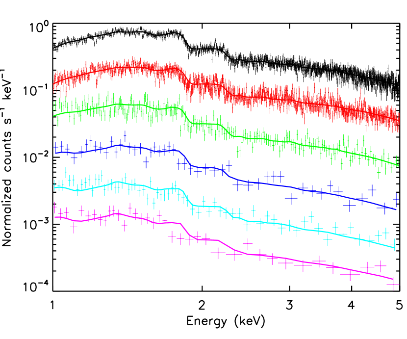
Figure 2: Data and spectral fits including PSF-correction for each annular region, illustrating the softening of the spectra with increasing radius. The regions plotted are $0^{\prime}-2.5^{\prime}$ (black), $2.5^{\prime}-6^{\prime}$ (red), $6^{\prime}-9.5^{\prime}$ (green), $9.5^{\prime}-13.5^{\prime}$ (blue), $13.5^{\prime}-18.5^{\prime}$ (cyan), and $>18.5^{\prime}$ (magenta). Data have been rebinned to a minimum significance of $5\sigma$ for each point, and each spectrum has been arbitrarily renormalized for visual clarity.

Figure 3: Same as Fig. 2, but with residuals to show the quality of the spectral fits, and with the Lockman Hole background spectrum included for comparison. Count levels have not been renormalized and we note that the regions have different areas and exposure times. Dotted and dashed curves represent the background (CXB+thermal) and cluster emission models, respectively.

4 Results

4.1 Temperature, density, and entropy profiles

Temperature and density profiles are the primary data products of X-ray observations of clusters, from which other properties including entropy, mass, and gas fraction profiles can be derived. We obtain the density from the normalization of the best-fitting thermal plasma model which is proportional to the emission measure, $\int{n_{\rm e}n_{\rm H}\,dV}$, where $n_{\rm e}\approx 1.2n_{\rm H}$ for typical abundances. We use the simpifying assumption of constant density within each annulus, and estimate the volume as that of the intersection between cylindical and spherical shells with shared inner and outer radii, $V=(4\pi/3)(r_{\rm out}^{2}-r_{\rm in}^{2})^{3/2}$, scaled by the fraction of the projected annulus observed. With the density and temperature determined, we can calculate the entropy profile, $K=kT/n_{\rm e}^{2/3}$. Each of these profiles is shown in Fig. 4.

Figure 4: Projected temperature, density, and entropy profiles. The vertical dashed line shows our estimate of $r_{200}$, derived in Section 4.2.

The cool core, though blurred by the wide PSF, is seen as a decrease in temperature near the center. The more novel result is the clearly-observed decline in temperature in the outskirts of the cluster. Excluding the core, this decline can be fit with a power law $T(r)=T_{0}r^{\alpha_{T}}$ with index $\alpha_{T}=-0.94\pm 0.06$. The gas density profile can similarly be fit with a power law, excluding the central region again for uniformity, with index $\alpha_{n}=-2.23\pm 0.01$. If we assume a polytropic distribution for an ideal gas, $P\propto n_{\rm H}kT\propto n_{\rm H}^{\Gamma}$, then we find $\Gamma=1+(\alpha_{T}/\alpha_{n})=1.42\pm 0.03$. This value is higher than that found for cooling flow clusters determined by e.g., De Grandi & Molendi (2002), who measured $\Gamma\simeq 1.2$ in the radial range $0.2r_{180}<r\lesssim 0.6r_{180}$.

Gas with high entropy rises, so the radial entropy profile is expected to increase. Puzzlingly, the entropy profile we observe rises from the center and then appears to level off beyond $\sim 10^{\prime}$, putting it on the border of convective instability. We will discuss possible explanations for this behavior in later sections.

4.2 Mass profiles

To derive a mass profile, we assume that the gas properties are spherically symmetric and that the cluster is in hydrostatic equilibrium. Balancing the thermal pressure gradient against the gravitational potential, we obtain an expression for the total gravitating mass in terms of temperature and density:

$$M(<r)=\frac{-kr^{2}}{G\mu m_{\rm H}n_{\rm H}}\left(T\frac{dn_{\rm H}}{dr}+n_{\rm H}\frac{dT}{dr}\right).$$ (1)

We assume that the total density distribution can be described by an NFW profile,

$$\rho(r)=\frac{\rho_{0}}{r/r_{\rm s}\left(1+(r/r_{\rm s})\right)^{2}},$$ (2)

where $\rho_{0}$ is a density normalization and $r_{\rm s}$ is a scale radius related to the cluster’s concentration, $c_{200}\equiv r_{200}/r_{\rm s}$.

Following an approach similar to that of Schmidt & Allen (2007), we use an NFW model and the observed gas density distribution to predict a temperature in each annulus, beginning with the outermost bin. Density gradients are taken linearly between the radial bins, which reduces the correlation in uncertainties between non-adjacent data points that are created with other interpolations such as cubic splines, as some authors use (see Voigt & Fabian, 2006, for a discussion). This approach could be improved with more radial bins, but the wide PSF of Suzaku and the low count rate in the cluster outskirts limit us from using thinner annular regions. To ensure that the outermost temperature value is robustly estimated, we take the median outer value of the profiles that best fit 100 Monte Carlo realizations of the observed temperature profile, normally distributed within its error bars. The model temperature profiles are similar if we begin at the innermost region, so the result is not particularly sensitive to the boundary values. Iterating over a range of NFW parameters, we select the mass model that produces the temperatures that best fit the observed profile.

In order to resolve the region within the NFW scale radius, we supplement the Suzaku data with an archival $20{\rm\thinspace ks}$ Chandra observation (ID 2427) taken with the ACIS-S detector in VFAINT mode. These data were reduced following the description of O’Dea et al. (2008), with spectra extracted in circular annuli and deprojected using the method of Sanders & Fabian (2007). After using the outermost Chandra annulus to subtract contaminating flux from inner regions it is omitted from further analysis since it may contain external cluster emission, leaving six regions to replace the innermost Suzaku bin, where the temperature and density is in reasonable agreement with the Chandra data. We use Chandra data for its sharper PSF, but the XMM temperature profile in Snowden et al. (2008) is also consistent at the smaller radii of that observation.

The model temperature profile, shown in Fig. 5, does not fit the data very well over all annuli, and the best fit to the observed temperatures ($\chi^{2}\approx 39$ for 7 degrees of freedom) is obtained after ignoring the outermost Suzaku bin which is beyond the virial radius where the assumption of hydrostatic equilibirium is expected to fail, and the Chandra regions in the cool core within $\sim 70{\rm\thinspace kpc}$ of the center where the gas is likely to be multiply-phased. The main deviation in our data from this acceptable temperature fit arises from the $2.5^{\prime}-6^{\prime}$ Suzaku annulus. Possible explanations include a PSF-correction that could be too large, a cross-calibration issue between Chandra and Suzaku, or even non-gravitational heating in that region.

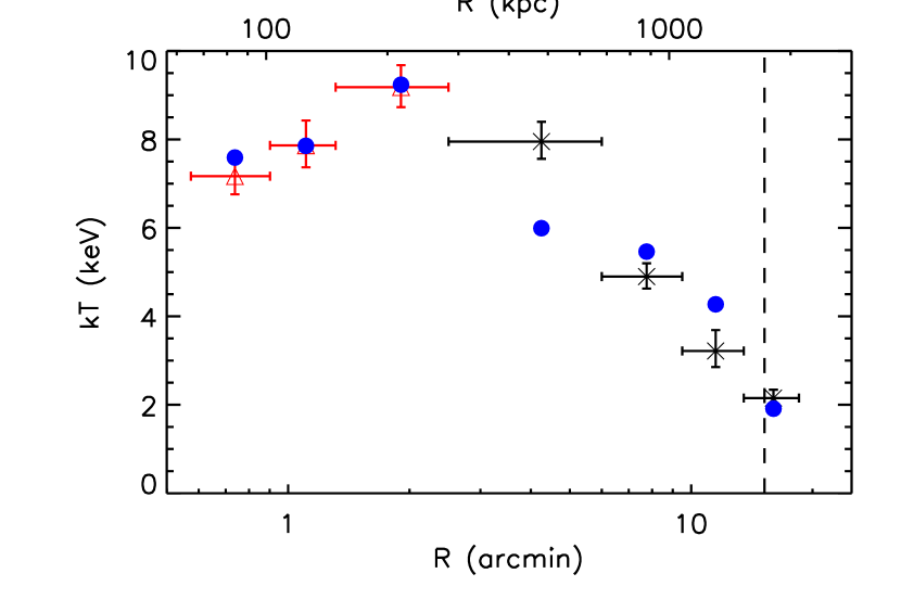
Figure 5: Chandra (red triangles) and Suzaku (black crosses) temperature values used in mass fitting analysis, along with matching temperatures for best fitting NFW profile (blue circles).

The resulting mass profile has best-fitting NFW parameters of $c_{200}=7.5^{+1.1}_{-0.9}$ and $r_{\rm s}=230^{+40}_{-40}{\rm\thinspace kpc}$, producing a virial radius $r_{200}=c_{200}r_{\rm s}=1.72\pm 0.06{\rm\thinspace Mpc}$, or $15.2^{\prime}$ and mass $M_{200}=200\rho_{c}(z)(4\pi/3)(r_{200})^{3}=6.4\pm 0.6\times 10^{14}{\rm\thinspace M_{\odot}}$ . We estimate the total uncertainty on the virial mass, including systematics, of $30\%$, which is described further in the next section. We compare these values with previous determinations in Table 3 and plot the mass profile in Fig. 6, along with the cumulative gas mass profile obtained from the power-law fit to the Suzaku gas density profile.

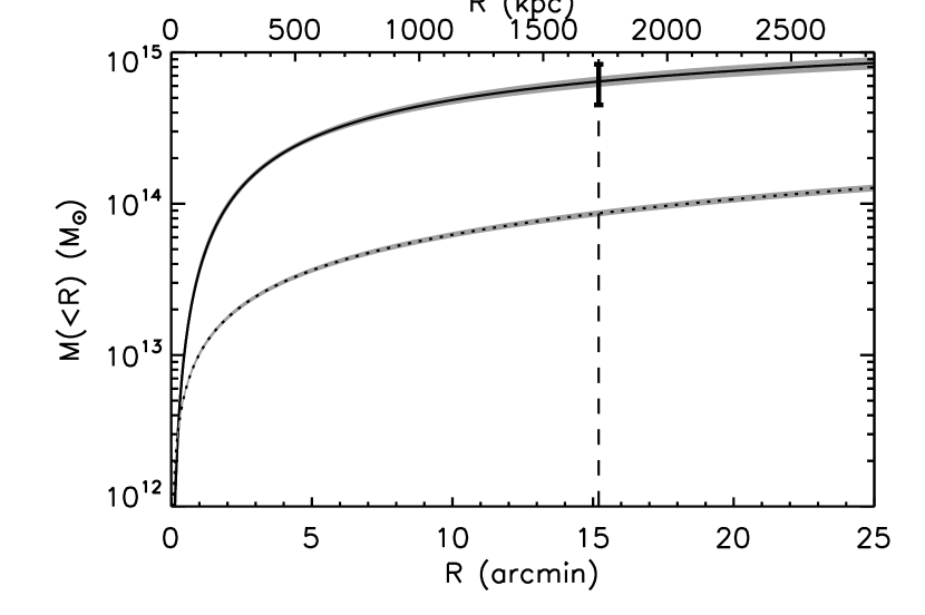
Figure 6: Cumulative profiles of gas mass (dotted lower curve) and total gravitational mass (solid upper curve) with $1\sigma$ statistical error ranges in gray. The single error bar shows the $30\%$ systematic uncertainty on $M_{200}$ and the vertical dashed line shows our estimate of $r_{200}$, derived in Section 4.2.

$c_{200}$	$M_{200}(10^{14}{\rm\thinspace M_{\odot}})$	Reference
$3.83^{+0.52}_{-0.27}$	$18.6^{+3.5}_{-4.0}$	Allen et al. (2003)
$5.12^{+0.40}_{-0.40}$	$10.0^{+1.2}_{-1.2}$	Pointecouteau et al. (2005)
$5.46^{+3.22}_{-2.88}$	$9.7^{+52.2}_{-8.5}$	Voigt & Fabian (2006)
$5.86^{+1.56}_{-1.07}$	$11.82^{+4.70}_{-3.55}$	Schmidt & Allen (2007)
$7.5^{+1.1}_{-0.9}$	$6.4^{+0.6}_{-0.6}$	This work

Table 3: Concentration and virial mass determinations for PKS 0745-191, compiled by Comerford & Natarajan (2007) with values for this work added.

The NFW concentration is higher than previous estimates, and the virial mass we determine is lower, due in part to the smaller virial radius found in this work. Reiprich & Böhringer (2002), who used an isothermal fit to ROSAT and ASCA data and found a value of $1.95\pm 0.03{\rm\thinspace Mpc}$ updated to the cosmological parameters we adopt. Schmidt & Allen (2007) found an even larger value for the virial radius, fitting an NFW profile to Chandra data in the central region to obtain $r_{200}\approx 2.2{\rm\thinspace Mpc}$. One issue with past NFW fits used to calculate the virial radius is that the data often do not extend even to the NFW scale radius, let alone the virial radius.

We can compare our mass profile with the projected mass determined from a strong lensing arc of radius $34.5{\rm\thinspace kpc}$ seen with Hubble imagery by Allen et al. (1996). Updating their mass estimate for the circular lens model to account for the current cosmological parameters, we expect a mass of $6.4\times 10^{12}{\rm\thinspace M_{\odot}}$ projected within a cylinder along the line of sight of the center of the cluster with a radius of the lensing arc, which is consistent with the statistical and systematic uncertainties of our best-fitting NFW model when integrating the mass in the cylinder out to $r_{200}$. We note that this includes an extrapolation of our profile into the core region where we have excluded data from our fit because of nonthermal processes. While it is reassuring to see this reasonable agreement between separate mass estimates, we caution that comparisons of this type of wide-field X-ray analysis with strong lensing data only involve a small fraction of the total cluster mass. Weak lensing analyses, which can provide mass projections over a much broader area, will provide important comparisons for virial mass estimates.

In Fig. 7, we plot the gas fraction profile, defined as the fraction of mass within a given radius composed of X-ray emitting gas. The gas fraction appears to rise slightly at the outer radii, consistent with the profile observed for PKS 0745-191 in ROSAT data by Allen et al. (1996). The values of the $f_{\rm gas}$ profile in the outskirts of this cluster are similar to recent measurements of the mean cosmic baryon fraction (Komatsu et al., 2008).

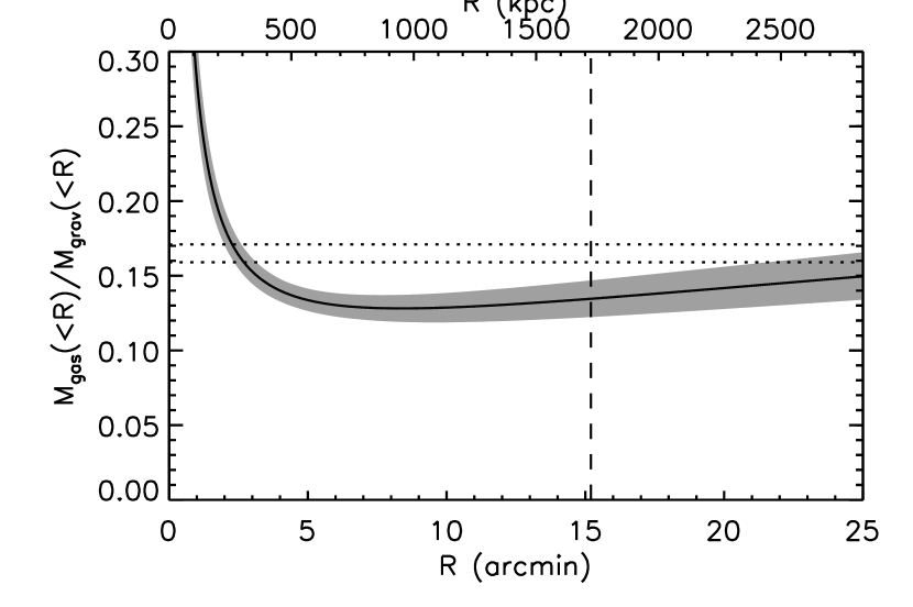
Figure 7: Gas fraction profile for PKS 0745-191, the ratio of the dotted to solid curves in Fig. 6, with $1\sigma$ statistical error range in gray. Dotted lines show the $1\sigma$ range around the value of $\Omega_{\rm b}/\Omega_{\rm m}$ from Komatsu et al. (2008). The vertical dashed line shows our estimate of $r_{200}$, derived in Section 4.2.

4.3 Uncertainties

Radius	kT	Stat.	No PSF	NXB	CXB	Gal.	${N_{\rm H}}$	Z
(’)	(${\rm\thinspace keV}$)			$\pm 3\%$	$\pm 10\%$	$\pm 50\%$	$\pm 10\%$	$0.2-0.4{\rm\thinspace Z_{\odot}}$
0–2.5	6.92	${}^{+0.12}_{-0.12}$	$+0.08$	$<0.005$	$<0.005$	$<0.005$	$0.68$	$<0.005$
2.5–6.0	7.85	${}^{+0.45}_{-0.39}$	$-0.82$	$<0.005$	$<0.005$	$0.01$	$0.90$	$0.02$
6.0–9.5	4.90	${}^{+0.30}_{-0.27}$	$-0.01$	$0.02$	$0.04$	$0.03$	$0.41$	$0.05$
9.5–13.5	3.22	${}^{+0.47}_{-0.36}$	$-0.05$	$0.14$	$0.14$	$0.06$	$0.28$	$0.07$
13.5–18.5	2.15	${}^{+0.19}_{-0.18}$	$+0.09$	$0.06$	$0.17$	$0.06$	$0.15$	$0.11$
$>18.5$	2.07	${}^{+0.25}_{-0.23}$	$+0.02$	$0.10$	$0.21$	$0.06$	$0.13$	$0.12$

Table 4: Estimated uncertainties in the radial temperature profile due to removing PSF-corrections or changing normalizations of background components and spectral model parameters within the ranges given. Each parameter is varied independently and we present only the maximum of the upward and downward temperature shifts (in ${\rm\thinspace keV}$) for clarity. Best-fitting PSF-corrected temperatures and their statistical uncertainties are included for comparison.

A number of systematic uncertainties could add contributions to our error budget beyond the statistical ranges plotted. We summarize our estimates of several of these systematic uncertainties to the temperature profile, including the effects of PSF-correction and renormalization of background components, in Table 4. The changes due to the PSF-correction are mostly small, with the main effect being a $\sim 12$ per cent increase in temperature in the second innermost annulus after accounting for emission from the cool gas in the core that has scattered outward. There is a significant uncertainty in the temperature of the central region because Suzaku’s PSF blurs the steep gradient of the cool core. As Reiprich et al. (2008) points out, the approach to PSF-corrections described in the previous section does not fully account for this blurring within the central region, however our method provides a reasonable approximation to the corrections needed.

To ensure that the background models used do not significantly impact the results, we vary the normalizations of these components and measure the deviations produced in temperature. The uncertainty in the NXB is $\sim 3$ per cent (Tawa et al., 2008), and from an analysis of ROSAT data by Carrera, Fabian & Barcons (1997), we estimate that the cosmic variance due to point source clustering in the CXB is $\sim 10$ per cent over this field of view. We also test the effect of metallicity from $0.2-0.4{\rm\thinspace Z_{\odot}}$ in the outer annuli and a range of $\pm 10$ percent in the column density. Each of these variations results in a change in temperature of $\lesssim 10$ per cent for all annuli, and the individual systematic uncertainties are smaller than the Poisson uncertainties for all but the column density’s effect on the central regions where the count rate is high. Finally, the normalization of the local thermal component, which could vary the most across the cluster field of view because of the low Galactic latitude, actually has a very small effect on temperature fits above $1{\rm\thinspace keV}$.

Without spectral deprojection, the data from each annulus will be contaminated by emission from regions at larger radii. But because the density profile falls so steeply and the thermal bremsstrahlung emission scales as the square of the density, the only noticeable effect is in the cluster core (e.g., Fig. 3 of Sanders & Fabian, 2007). This region is well within our innermost radial bin, so we do not expect significant errors due to the lack of deprojection of the Suzaku data.

As an additional check on the reliability of our temperature and density profiles, we compare the values from Suzaku with the Chandra observations used in the mass estimate. The high spatial resolution of Chandra allows for our central region to be divided into several annuli, with the average temperature in agreement with the Suzaku value. As shown in Fig. 8, the density profiles are also reasonably consistent between the two observatories, with a slightly steepening slope at the larger radii seen by Suzaku.

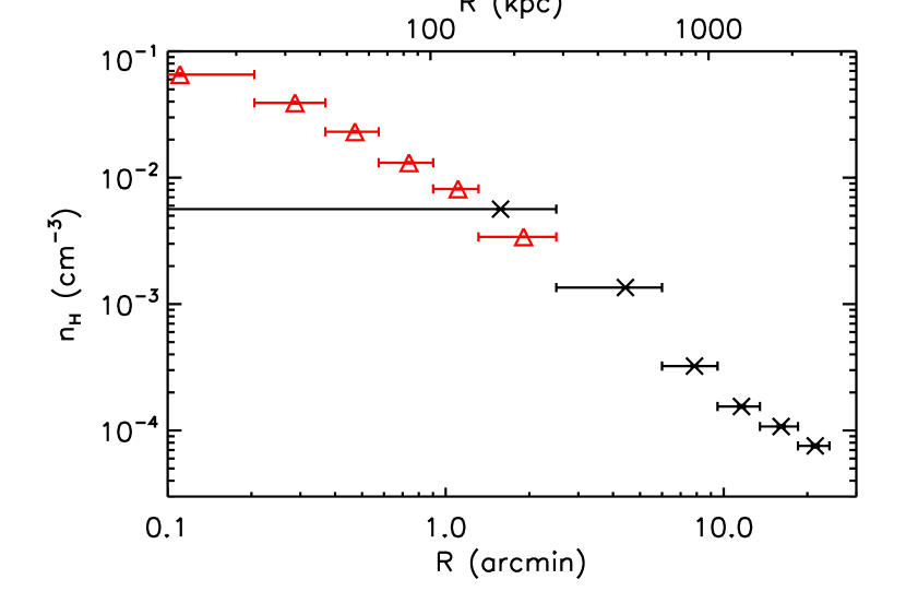
Figure 8: Comparison between Chandra (red triangles) and Suzaku (black crosses) density profiles. Error bars are smaller than the plot symbols.

We can check the assumption of spherical symmetry used when deriving the mass profile, seeing if the emission is at least circularly symmetric by considering the projected profiles in each of the pointings separately. Fig. 9 shows the temperature, density, and entropy profiles for each pointing. Here we do not include PSF-corrections in order to keep each set of observations independent. The uncertainties are larger when splitting up the data, but the results from the separate pointings broadly overlap, and no single direction is consistently above or below the average temperature or density for every annulus. Scatter that is larger than the statistical uncertainties could be attributed to remaining point sources or minor asymmetry in the cluster.

The entropy seen in the outermost radial bin of the NW pointing is significantly lower than nearby regions, mainly due to the temperature drop seen there. However, scatter between pointings or individual outliers are unable to explain the observed flattening of the entropy profile in the summed annuli. We plot a power law rising as $r^{1.1}$ to compare with the entropy profile predicted by analytical models of accretion shock heating and seen in some observations as well as numerical simulations (Tozzi & Norman, 2001; Ponman et al., 2003; Voit et al., 2005). A small number of objects in the sample of Ponman et al. (2003) have entropy curves that do not rise with radius. The observed and expected profiles agree at small radii, rising out of the core, but there is a clear entropy deficit in the outskirts of the cluster, perhaps indicative of infalling gas which is not dynamically stable. Our background model would have to be off by an order of magnitude, or the column density changed by a factor of 2, to increase the entropy in the outskirts to the predicted values.

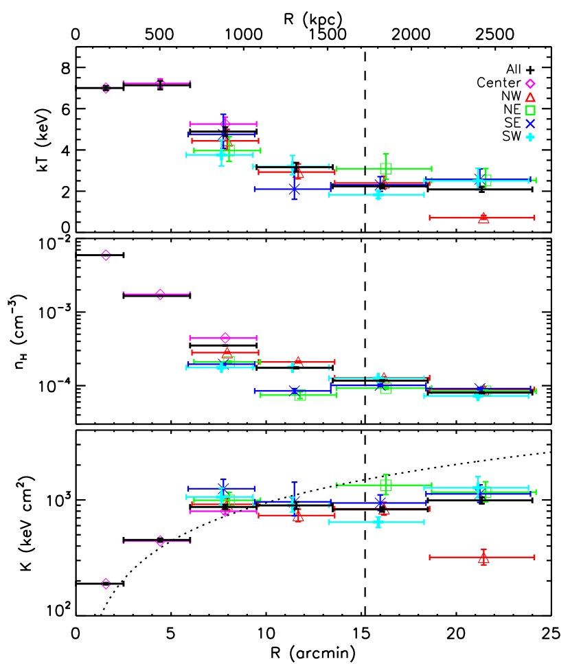
Figure 9: Comparison of temperature, density, and entropy profiles in each direction. The temperature in the NE direction is not well-constrained from $9.5^{\prime}-13.5^{\prime}$ due to a large amount of area excluded because of point sources, so the temperature and entropy points are not plotted in this region. Slight offsets are added to bin radii for clarity. The dotted curve in the bottom panel shows $K\propto r^{1.1}$. The vertical dashed line shows our estimate of $r_{200}$, derived in Section 4.2.

For the estimates of the virial radius and mass, the method of fitting an NFW model to our temperature profile is an additional source of uncertainty. We have excluded the inner and outer regions where the assumption of hydrostatic equilibrium is likely to break down, but several variations of the temperature profile with these points included or excluded produce values for $r_{200}$ consistent to $\sim 10$ per cent. Similar values are also obtained when using only the Suzaku data, which has a large uncertainty in the central temperature due to PSF-blurring. The wide radial span of this data set provides significantly tighter constraints on the NFW parameters than could be obtained with the Chandra data alone, as shown in Fig. 10. Data from the cluster core are still excluded in the contours plotted, though they might be used in a typical analysis. In either case with only Chandra data, the NFW scale radius is not well-constrained since the data do not extend out that far, and the resulting estimate for $r_{200}$, and thus $M_{200}$, would be significantly larger than the values we obtain. We can also include the systematic uncertainties in the temperature profile within this process of fitting over NFW parameter space. Even with differences of $0.5-1{\rm\thinspace keV}$ between the FI and BI sensors which have similarly shaped but offset temperature profiles, changes in the best fitting value of $R_{200}$ are of order $10\%$, giving a systematic uncertainty of $30\%$ for the determination of $M_{200}$.

We can also estimate the cluster mass independently of any model parametrization by plugging our density and temperature profiles directly into Equation 1 and calculating gradients from the finite difference quotients of adjacent points. At large radii, the cumulative mass estimate using this method actually decreases, indicating that the hydrostatic assumption fails, and the uncertainties are large because spatial gradients are taken between points separated by the wide thickness of annular bins. However, at the virial radius near $15^{\prime}$, the mass estimate agrees with that derived from the NFW model to within $\sim 30$ per cent.

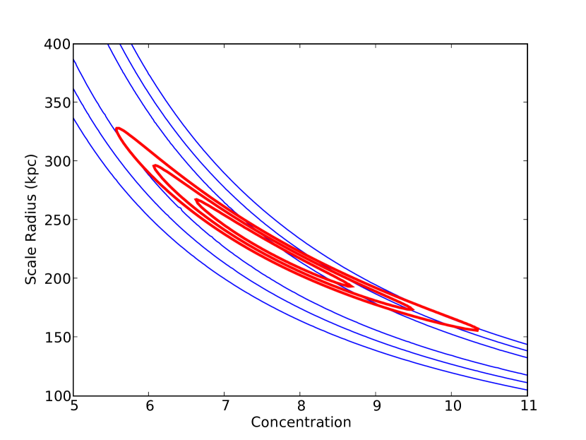
Figure 10: Likelihood contours for the concentration and scale radius parameters of the NFW fits, drawn at $\Delta\chi^{2}=2.30$, 6.17, and 11.80, corresponding to the $1\sigma$, $2\sigma$, and $3\sigma$ confidence intervals, respectively. Thick red contours show the constraints from the combination of Chandra and Suzaku data, excluding the cluster core and the outermost annulus which is beyond the virial radius. Thin blue contours show the constraints without the Suzaku data for comparison.

5 Discussion

These are the first well-constrained measurements of the gas temperature profile beyond $r_{200}$ for a rich and relaxed cluster, which we can now compare with model predictions and simulations. We see that there is a clear decline in temperature between $0.3-1.5r_{200}$, consistent with recent observational trends at growing radii (Vikhlinin et al., 2005; Pratt et al., 2007; Reiprich et al., 2008) and suggesting that conduction does not play a significant role on typical cluster time-scales. Roncarelli et al. (2006) measured the magnitude of the temperature drop in hydrodynamical simulations, finding a 40 per cent decline from $0.3-1r_{\rm 200}$, the same size found in the analytical treatment of Ostriker, Bode & Babul (2005). The drop observed in PKS 0745-191 over this radial range is closer to 70 per cent, but the general shapes of the profiles are similar.

The observed entropy profile deviates from expectations near the virial radius. Tozzi & Norman (2001) describe the effects on entropy of the accretion phases, including adiabatic infall, shock heating, and adiabatic compression followed by cooling within the halo. Interestingly, we see evidence for an accretion shock beyond the virial radius in one direction (NW pointing in Fig. 9), suggestive of cool material falling inward along a filament. The change in entropy in the outer annulus of this region is not seen in the other directions, though the values there are still lower than would be expected from the typical increase of $K\propto r^{1.1}$.

The sharper decline in temperature than predicted and the flattening of the entropy profile in the outskirts suggest a need for nonthermal pressure support in order to maintain dynamic stability. The numerical simulations of Eke, Navarro & Frenk (1998) show a significant rise in the ratio of bulk kinetic energy to thermal energy beginning within the virial radius. Merger activity increases the turbulent pressure, and even though PKS 0745-191 appears relaxed morphologically, it should still be accreting matter in the outskirts. We note that the infall time-scale, $t_{\rm f}\sim(r^{3}/GM)^{1/2}$, is of order $1{\rm\thinspace Gyr}$ at the virial radius, and the time-scale set by the speed of sound, $t_{\rm s}\sim(r^{2}m_{\rm H}/\Gamma kT)^{1/2}$, is several times larger.

Neumann (2005), studying the summed profiles of 14 nearby Abell clusters beyond $r_{200}$, argues that the ICM at large radii may not be in hydrostatic equilibrium, and that cool gas not seen in X-rays could increasingly dominate the baryon content in the outskirts. Afshordi et al. (2007) stacked WMAP observations of a large sample of massive clusters and found a deficit in thermal energy in the outskirts from the Sunyaev-Zel’dovich profile, also arguing for cool phase of the ICM. It is not well understood how these different phases would mix, and complicated gas physics would likely result. The assumption of hydrostatic equilibrium fails beyond the virial radius, as seen by the poorer temperature fits from mass modeling when the outermost temperature value is included. It is not obvious to what extent the ICM within the virial radius is not in equilibrium, but the entropy and temperature profiles suggest that nonthermal physics may be important in the outskirts of this cluster.

In Fig. 11, we plot the observed temperature profile against two models. The first is the expected temperature if the gas content traced the NFW distribution of dark matter, with a Keplerian velocity profile, i.e., $T(r)\propto v(r)^{2}\propto M(<r)/r$. The second and more realistic case is for the projected X-ray temperature of gas arranged polytropically and in hydrostatic equilibrium with an NFW gravitational potential, as derived by Suto, Sasaki & Makino (1998). The outer temperatures we have observed are lower than those expected for reasonable values of the model parameters. Additionally, we can fit the observed temperature profile using a simple parametrization

$$T(r)=T_{1}\left(\frac{r}{r_{s}}\right)^{\alpha}\left(1+\frac{r}{r_{s}}\right)^{\beta}\rm keV$$ (3)

with best-fitting parameters $T_{1}=135$, $\alpha=2.4$, $\beta=-4.1$, where $r_{\rm s}$ is the scale radius from the best-fitting NFW profile. We note that the normalization is related to the value of the temperature at this radius, $T_{1}=T(r_{\rm s})/2^{\beta}$.

A possible explanation for the deficit of thermal energy seen at large radii is that infalling matter has retained some of its kinetic energy in bulk motion. If there is increasing pressure support from bulk motion, turbulence, or other nonthermal processes in the outer regions of the cluster, then the gravitational potential and thus total mass would be incorrectly estimated when assuming hydrostatic equilibrium. This effect would depend on the changes in both the temperature and its gradient, making estimation of the true mass difficult.

Alternatively, the peak temperature, seen in the second-innermost annulus, could be inflated due to nonthermal processes such as shock heating during infall. AGN heating is thought to play an important role in cool core clusters, and some excess energy could also heat the gas beyond the core. More observations are needed of this cluster and others to determine how well the self-similar scaling relations, which depend on the dominance of gravitational process in creating equilibrium, apply out to the virial radius.

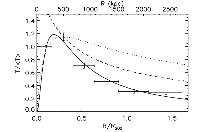
Figure 11: Suzaku temperature profile, normalized by the emission-weighted mean and compared with model profiles. The solid curve shows the parametrization of Equation 3, also rescaled by the emission-weighted mean temperature that we observe. The dotted curve shows the temperature for gas tracing an NFW distribution, while the dashed curve shows a polytropic profile in hydrostatic equilibrium with an NFW potential. Both models are normalized to match the maximum observed temperature.

The gas fraction we obtain is more consistent with previous results. At $r_{200}$, $f_{\rm gas}=0.13$, lower than that found with XMM (Chen et al., 2003), but similar to the ROSAT value of Allen et al. (1996). The trend of $f_{\rm gas}$ rising with radius is also seen in other clusters and in simulations (e.g., Vikhlinin et al., 2006; Eke et al., 1998), since the gas density distribution is less centrally concentrated than that for collisionless dark matter. The outermost measured value of $f_{\rm gas}$ is consistent with the mean cosmic baryon ratio derived from WMAP data and other cosmological observations, $\Omega_{\rm b}/\Omega_{\rm m}=0.165\pm 0.006$ (Komatsu et al., 2008).

6 Summary

We have presented the first measurements of the gas beyond the virial radius from a rich and apparently relaxed galaxy cluster. The temperature profile shows a significant decline at outer radii, while the entropy profile levels off. The spatially resolved temperature and density measurements out to and beyond the virial radius produce improved constraints on the mass and gas fraction profiles, though the observed temperature profile does show deviations from that expected from cluster gas in hydrostatic equilibrium with an NFW mass profile.

Observations of the outskirts of clusters offer a direct probe of their assembly history. The apparent shock front in one direction makes it clear that this cluster is still accreting material, likely along a filament. Evidence for nonthermal pressure support suggests that bulk motions from merger activity could be making a significant contribution to the gas energy in the outskirts of this cluster.

PKS 0745-191 is an ideal candidate for such observations, given its distance and luminosity. The angular size fits reasonably within a few pointings and the count rate is high enough for good spectral statistics. The low and well-constrained background levels of Suzaku are crucial for low surface brightness measurements like those presented here and by Reiprich et al. (2008). We expect that as the number of cluster observations in the Suzaku archive increases, these types of analyses will be able to probe the self-similarity of the outskirts of clusters. More studies at the virial radius, including X-ray observations, gravitational lensing, the SZ effect, and numerical simulations, will provide a better understanding of the regime where hydrostatic equilibrium breaks down and clusters are still being assembled.

References

- Afshordi et al. (2007) Afshordi N., Lin Y.-T., Nagai D., Sanderson A. J. R., 2007, MNRAS, 378, 293
- Allen et al. (1996) Allen S. W., Fabian A. C., Kneib J. P., 1996, MNRAS, 279, 615
- Allen et al. (2008) Allen S. W., Rapetti D. A., Schmidt R. W., Ebeling H., Morris R. G., Fabian A. C., 2008, MNRAS, 383, 879
- Allen et al. (2003) Allen S. W., Schmidt R. W., Fabian A. C., Ebeling H., 2003, MNRAS, 342, 287
- Anders & Grevesse (1989) Anders E., Grevesse N., 1989, Geochim. Cosmochim. Acta, 53, 197
- Arnaud et al. (2005) Arnaud M., Pointecouteau E., Pratt G. W., 2005, A&A, 441, 893
- Carrera et al. (1997) Carrera F. J., Fabian A. C., Barcons X., 1997, MNRAS, 285, 820
- Cash (1979) Cash W., 1979, ApJ, 228, 939
- Chen et al. (2003) Chen Y., Ikebe Y., Böhringer H., 2003, A&A, 407, 41
- Comerford & Natarajan (2007) Comerford J. M., Natarajan P., 2007, MNRAS, 379, 190
- De Grandi & Molendi (2002) De Grandi S., Molendi S., 2002, ApJ, 567, 163
- Edge et al. (1990) Edge A. C., Stewart G. C., Fabian A. C., Arnaud K. A., 1990, MNRAS, 245, 559
- Eke et al. (1996) Eke V. R., Cole S., Frenk C. S., 1996, MNRAS, 282, 263
- Eke et al. (1998) Eke V. R., Navarro J. F., Frenk C. S., 1998, ApJ, 503, 569
- Evrard et al. (1996) Evrard A. E., Metzler C. A., Navarro J. F., 1996, ApJ, 469, 494
- Fabian et al. (1985) Fabian A. C., et al., 1985, MNRAS, 216, 923
- Frenk et al. (1999) Frenk C. S., et al., 1999, ApJ, 525, 554
- Fujimoto et al. (2007) Fujimoto R., et al., 2007, PASJ, 59, 133
- Irwin et al. (1999) Irwin J. A., Bregman J. N., Evrard A. E., 1999, ApJ, 519, 518
- Ishisaki et al. (2007) Ishisaki Y., et al., 2007, PASJ, 59, 113
- Kaiser (1986) Kaiser N., 1986, MNRAS, 222, 323
- Kalberla et al. (2005) Kalberla P. M. W., Burton W. B., Hartmann D., Arnal E. M., Bajaja E., Morras R., Pöppel W. G. L., 2005, A&A, 440, 775
- Komatsu et al. (2008) Komatsu E., et al., 2008, preprint (arxiv:0803.0547)
- Koyama et al. (2007) Koyama K., et al., 2007, PASJ, 59, 23
- Liedahl et al. (1995) Liedahl D. A., Osterheld A. L., Goldstein W. H., 1995, ApJ, 438, L115
- Loken et al. (2002) Loken C., Norman M. L., Nelson E., Burns J., Bryan G. L., Motl P., 2002, ApJ, 579, 571
- Markevitch et al. (1998) Markevitch M., Forman W. R., Sarazin C. L., Vikhlinin A., 1998, ApJ, 503, 77
- McLaughlin (1999) McLaughlin D. E., 1999, AJ, 117, 2398
- Mewe et al. (1985) Mewe R., Gronenschild E. H. B. M., van den Oord G. H. J., 1985, A&AS, 62, 197
- Mewe et al. (1986) Mewe R., Lemen J. R., van den Oord G. H. J., 1986, A&AS, 65, 511
- Navarro et al. (1997) Navarro J. F., Frenk C. S., White S. D. M., 1997, ApJ, 490, 493
- Neumann (2005) Neumann D. M., 2005, A&A, 439, 465
- O’Dea et al. (2008) O’Dea C. P., et al., 2008, ApJ, 681, 1035
- Ostriker et al. (2005) Ostriker J. P., Bode P., Babul A., 2005, ApJ, 634, 964