Polariton lasing in a multilevel quantum dot
strongly coupled to a single photon mode

Abstract

We present an approximate analytic expression for the photoluminescence spectral function of a model polariton system, which describes a quantum dot, with a finite number of fermionic levels, strongly interacting with the lowest photon mode of a pillar microcavity. Energy eigenvalues and wavefunctions of the electron-hole-photon system are obtained by numerically diagonalizing the Hamiltonian. Pumping and photon losses through the cavity mirrors are described with a master equation, which is solved in order to determine the stationary density matrix. The photon first-order correlation function, from which the spectral function is found, is computed with the help of the Quantum Regression Theorem. The spectral function qualitatively describes the polariton lasing regime in the model, corresponding to pumping rates two orders of magnitude lower than those needed for ordinary (photon) lasing. The second-order coherence functions for the photon and the electron-hole subsystems are computed as functions of the pumping rate.

I Introduction

Excitonic polaritons are quasiparticles made up from strongly coupled electron-hole pairs and photonspolaritons1 ; polaritons2 . They are experimentally realized in semiconductor optical microcavities with embedded quantum wells. The small volume of the microcavity, high reflectivity of its walls, and quasiresonance condition between the confined-photon and excitonic energies guarantee the strong coupling regime.

At very-low excitation rates, in mean only a single quasiparticle lives inside the cavity. With increasing excitation power, however, an abrupt increase of ground-state occupation takes place due to the quasibosonic statistics of the polaritons. A threshold behaviour of the photoluminescence is observed. This behaviour has been interpreted as Bose-Einstein condensation of polaritons Yamamoto ; LeSiDang or as a dynamical effect (polariton lasing)JBloch . The latter position is motivated by the experimental demonstration that thermalization mechanisms are not effective.

In the present paper, we start from the idea of the polariton laser Imamoglu , where pumping provides a reservoir from which the low-lying polariton states are populated. Unlike common lasers, no population inversion is required and the active medium (the excitons) is strongly interacting with the cavity photons, forming the quasibosonic polaritons.

The theoretical description of polaritons faces the difficulties inherent to a many-particle strongly-interacting system working under a non-equilibrium pumping regime. Our strategy to tackle this problem is based upon two simplifications. First, we consider a finite system PhysE35(2006)99 ; nuestraPRL ; distortedGibbs , that is a single photon mode, and a finite number of single-particle states (ten) for electrons and holes. Then, the electron-hole-photon many-particle Hamiltonian is numerically diagonalized in order to find the energies and wavefunctions of the system. We stress that both Coulomb and electron-hole-photon interactions are treated exactly in our scheme. Second, we compute the stationary density matrix from a master equation which accounts for photon losses through the cavity mirrors and pumping. The master equation is solved in a truncated set of many-particle states. Notice that these simplifications preserve the main ingredients of the problem: the existence of fermionic and bosonic degrees of freedom, the strong coupling between them, the existence of a finite number of single-particle states for fermions (around $10^{4}$ in Ref. [JBloch, ], 10 in our model) participating in the conformation of polaritons, a stationary state reached when pumping and losses are equilibrated, etc.

Strictly speaking, our model describes a quantum dot supporting a few excitonic states and strongly interacting with the lowest photon mode of a thin micropillar. It covers an intermediate region between the two-level dot Tejedor1 ; Tejedor2 ; Tejedor3 and the infinite system (well) previos . It is simple enough to allow exact diagonalization but, at the same time, complex enough to capture many of the properties of the infinite system.

The plan of the paper is as follows. In Sec. II, the model is described in details. In the next section, we briefly sketch the algorithm for the numerical diagonalization of the Hamiltonian, and show a few results for the energy spectrum and matrix elements of operators. In Sec. IV, we present the master equation for the density matrix and show typical occupations of many-polariton levels for low, intermediate, and relatively strong pumping rates. In Sec. V, the way of obtaining the exact photoluminescence (PL) spectral function, and the approximations leading to the simplified expression used in the paper are clarified. From this expression, we compute the intensity, position and linewidth of the main PL peak as functions of the pumping rate. Sec. VI is devoted to second-order coherence functions. Finally, in the last section, we summarize the main results of the paper.

II The model polariton system

As mentioned in the preceding section, we study a finite polariton system. A GaAs micropillar with radius of about one micron or lower is considered, in such a way that the lowest photon mode is well separated from the higher modes mp , and we can assume that a single photon mode is coupled to the lowest electron-hole states. The active medium inside the cavity is described by a finite number of harmonic-oscillator states for electrons and holes, as shown in Fig. 1. The number of single-particle states (ten) is dictated only by practical reasons: the dimension of the many-particle Hilbert space grows exponentially with the number of states. This finite system could be a good model for a quantum dot inside a thin micropillar, and even could be used to obtain the qualitative behaviour of quantum well-based micropillars.

The interaction Hamiltonian includes electron-electron, hole-hole, and electron-hole Coulomb interactions as well as electron-hole-photon coupling, the latter in the rotating-wave approximation HK :

$$H = \sum_{i}\left\{T^{(e)}_{i}e^{\dagger}_{i}e_{i}+T^{(h)}_{i}h^{\dagger}_{i}h_{i}\right\}$$ (1)

$$+ \frac{\beta}{2}\sum_{ijrs}\langle i,j||r,s\rangle~{}e^{\dagger}_{i}e^{\dagger}_{j}e_{s}e_{r}+\frac{\beta}{2}\sum_{ijrs}\langle i,j||r,s\rangle~{}h^{\dagger}_{i}h^{\dagger}_{j}h_{s}h_{r}$$

$$- \beta\sum_{ijrs}\langle i,j||r,s\rangle~{}e^{\dagger}_{i}h^{\dagger}_{j}h_{s}e_{r}+(E_{gap}+\Delta)~{}a^{\dagger}a$$

$$+ g\sum_{i}\left\{a^{\dagger}h_{\bar{i}}e_{i}+ae^{\dagger}_{i}h^{\dagger}_{\bar{i}}\right\}.$$

The effective band gap, $E_{gap}$, is taken as 1500 meV for GaAs. $\Delta$ is the detuning of the photon mode with respect to $E_{gap}$. The harmonic oscillator energies are much smaller than $E_{gap}$. We will neglect them in the single-particle energies of electrons and holes, and will write: $T_{i}^{(h)}=0$, $T_{i}^{(e)}=E_{gap}$. $g$ is the electron-hole-photon coupling strength. Notice that we are including only spin-up electrons, spin-down holes and one “circular” polarization of photons in Eq. (1). A model with the two photon polarizations, which, however, would dramatically increase the dimension of the Hilbert space, would make possible the study of interesting features such as the spontaneous build-up of coherence between “left-handed” and “right-handed” polaritons Kavokin . $\beta$ is the strength of Coulomb interactions, and $\langle i,j||r,s\rangle$ – the dimensionless matrix elements among harmonic oscillator states.

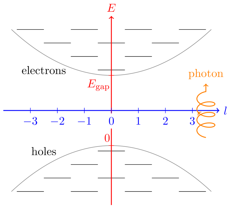
Figure 1: (Color online) Schematic representation of the harmonic oscillator states for electrons and holes in the model.

The oscillator states are labeled by two quantum numbers: the number of zeroes in the radial wave function, $k$, and the angular momentum projection along the cavity axis, $l$. The hole state, $\bar{i}$, in Eq. (1) is the conjugate of the electron state $i$, that is, has the same $k$, but the momentum is $-l$. This means that the photon interacts only with electron-hole pairs with zero angular momentum. As a consequence, the total angular momentum of the electron-hole system:

$$L=\sum_{i}\left(l_{i}^{(e)}+l_{i}^{(h)}\right),$$ (2)

is a conserved magnitude. In addition, the Hamiltonian, Eq. (1), preserves the polariton number:

$$N_{pol}=N_{pairs}+N_{ph}=\frac{1}{2}\sum_{i}\left(e_{i}^{\dagger}e_{i}+h_{i}^{\dagger}h_{i}\right)+a^{\dagger}a.$$ (3)

We notice the similarity between ours and a finite Dicke model Dicke . The infinite Dicke model has been used to describe polaritons in microcavities Littlewood . The main difference with our approach is the following. In the Dicke model of polaritons, we first solve for the excitons and retain only the ground state. Multiexcitonic states are not considered. This, may be, is a good approximation for far-appart, small (not supporting multiexcitons) quantum dots in a microcavity.

Figure 2: Polariton states with $N_{pol}=1$.

Many-particle states with fixed $N_{pol}$ and $L$ are constructed in the next section. We give here a preview in order to compare with the traditional picture of non-interacting polaritons. We take for the parameters the values, $g=3$ meV, and $\beta=2$ meV. The latter is a reasonable value for GaAs, leading to an exciton binding energy of a few meVs. The high value of $g$ is, however, not intended to be realistic. It is chosen in order to illustrate the interesting regime, not studied so far, where photon-pair coupling and Coulomb interactions are comparable. In Fig 2 we show all of the states with $N_{pol}=1$ in the model. We joined with a dashed line the lowest states in each $L$ tower (the yrast states) in order to conform the lower polariton (LP) branch. The upper polariton (UP) states, on the other hand, can be identified from the photoluminescence (PL) emission. We indicated in Fig. 2 the UP state in the $L=0$ sector. Notice that, because of the strong electron-hole-photon coupling constant, the UP state is pushed up to high energies in our model. In between LP and UP states there is a set of “dark” polariton states. They play an important role in the dynamics because they can not decay through photon emission. Let us stress that, our high-$g$ regime could be of interest in other contexts, where ultra-high light-matter couplings have been reported Aji .

We shall see in Sec. IV that photon losses in the cavity and incoherent pumping can be modeled by two terms in the master equation for the density matrix. We will not include relaxation mechanisms inducing transitions between states in the same $N_{pol}$ sector (acoustical phonons). As a result, the total angular momentum is conserved even when pumping and losses are taken into account. We will solve the dynamics in the $L=0$ tower, which will allow us to compute the PL emission along the pillar symmetry axis.

Finally, let us comment about the truncation of the basis of single-particle states in Fig. 1. For small quantum dots, this is a natural assumption. In thin micropillars, the number of states strongly coupled to the lowest photon mode is large, but finite. In Ref. JBloch, , for example, it should be around $10^{4}$. In this sense, our model may be thought of as a scaled version of a micropillar. At larger excitation energies the electron-hole states behave incoherently and act as a reservoir for the lower polariton states. We partially take account of these higher excited states in our model of incoherent pumping (Sec. IV). Coulomb interactions between polariton states and the reservoir, which is an additional source of decoherence, will be, however, neglected.

III Exact diagonalization results for the isolated system

For given $N_{pol}$ and $L$, we diagonalize the Hamiltonian in a basis constructed from Slater determinants for electrons and holes and Fock states of photons. The wave functions are looked for as linear combinations:

$$|I\rangle=\sum C_{S_{e},S_{h},n}|S_{e},S_{h},n\rangle.$$ (4)

where $S_{e}$ and $S_{h}$ are Slater determinants for electrons and holes with the same number of particles, $N_{pairs}$, and the number of photons is $n=N_{pol}-N_{pairs}$. When $N_{pol}=0$ there is only one state, the vacuum. When $N_{pol}=1$ there are 17 states with $L=0$. One of them is the state with one photon (no pairs), and the remaining 16 states correspond to matter excitations (no photons), that is, all possible combinations of one electron and one hole states with total angular momentum equal to zero. On the other hand, there are 256 states with $N_{pol}=2$, 1746 states with $N_{pol}=3$, etc. As $N_{pol}$ increases, the number of eigenstates of $H$ rises, reaching around 18000 for $N_{pol}\geq 10$. We use Lanczos algorithms Lanczos to obtain the energies and wavefunctions of the lowest states in each sector.

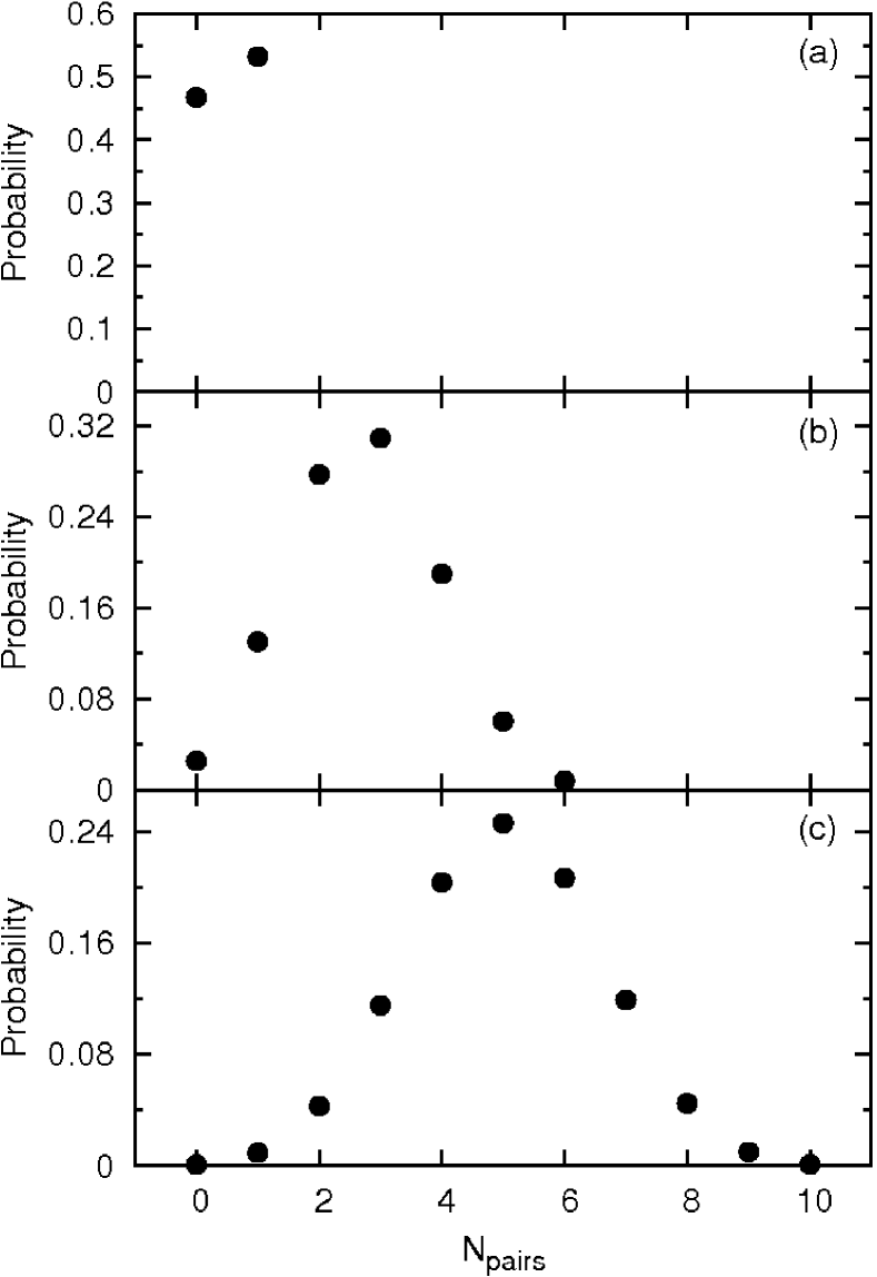
Figure 3: Weights of the sectors with given $N_{pairs}$ in the ground state wave functions. Case (a) corresponds to $L=0$ and $N_{pol}=1$, case (b) to $N_{pol}=6$, and case (c) to $N_{pol}=600$.

We give in Fig. 3 a schematic representation of the ground state wave functions with quantum number $L=0$, and polariton numbers $N_{pol}=1$ (case (a)), $N_{pol}=6$ (case (b)), and $N_{pol}=600$ (case (c)). The detuning parameter is fixed to $\Delta=-3$ meV. This value corresponds to quasi resonance. Indeed, in the $N_{pol}=6$ case, the distribution is peaked around $N_{pairs}=3$, whereas in the large-$N_{pol}$ limit it is peaked around $N_{pairs}=5$, that is the mean occupation of fermionic levels is near 1/2. Notice that the mean number of photons is around 595 in the latter case.

In Fig. 4 (a) the many-particle effects on polariton (photon) emission are made evident. We plotted the energy difference $E_{gs}(N_{pol})-E_{gs}(N_{pol}-1)-E_{gap}$ as a function of $N_{pol}$. A persistent blueshift towards the photon energy (equal to $\Delta$) is noticed as $N_{pol}$ is increased.

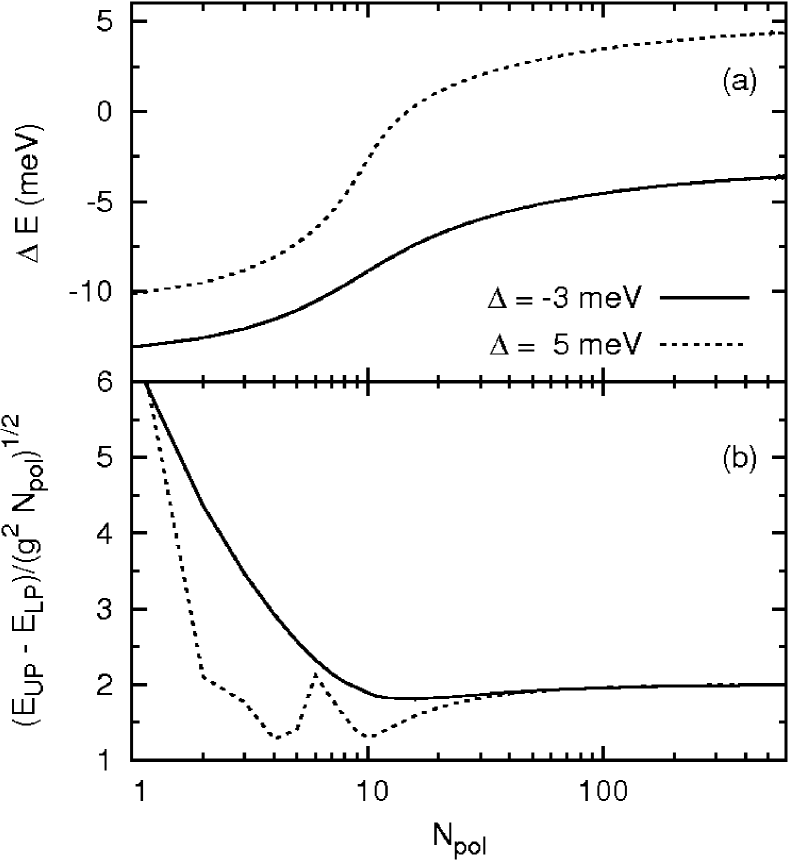
Figure 4: (a) Energy shift of photon emission from the ground state as a function of $N_{pol}$. That is, $\Delta E=E_{gs}(N_{pol})-E_{gs}(N_{pol}-1)-E_{gap}$. (b) Scaling in the $E_{UP}-E_{LP}$ energy difference.

On the other hand, in Fig. 4 (b) the energy difference $E_{UP}-E_{LP}$ is plotted as a function of $N_{pol}$. For large $N_{pol}$ numbers, this difference behaves like $2\sqrt{g^{2}N_{pol}}$.

The obtained wave functions may be used to compute matrix elements of operators. As it will be seen in the next section, the most important matrix elements related to photon emission and losses are $\langle F|a|I\rangle$, where the many-polariton states $F$ and $I$ are such that $N_{pol}(F)=N_{pol}(I)-1$. We show in Fig. 5 (a) the matrix elements squared $|\langle F|a|I\rangle|^{2}$ for transitions from $N_{pol}=2$ states to the one-polariton ground state. A Lorentzian with $\Gamma=0.1$ meV is used to smear out the transitions. The analogs of UP and LP states are also clearly distinguished here and in any $N_{pol}$ sector. The transfer of population from the UP state with $N_{pol}$ polaritons to the LP state with $N_{pol}-1$ polaritons will be a key ingredient in the dynamics, as will become clear in the next section.

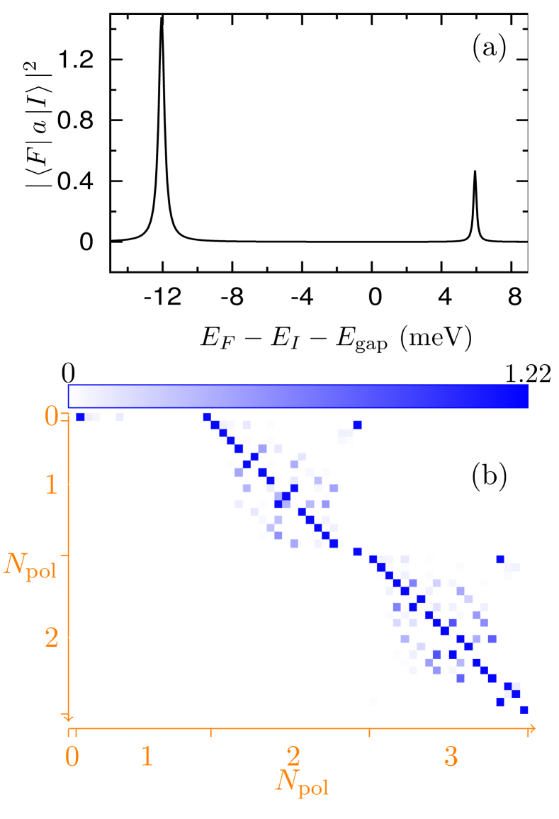
Figure 5: (Color online) (a) The matrix elements $|\langle F|a|I\rangle|^{2}$ for transitions from $N_{pol}=2$ states to the one-polariton ground state. A Lorentzian with $\Gamma=0.1$ meV is used to smear out the transitions. (b) The matrix $|\langle F|a|I\rangle|$ in the low-$N_{pol}$ sectors.

In Fig. 5 (b) we draw the absolute value of the matrix elements $|\langle F|a|I\rangle|$ in the low-$N_{pol}$ sectors. When $N_{pol}>1$, only the lowest 20 states are used to construct the matrix. Notice that the analogs of LP and UP states are always included among these 20 states. We computed the matrix elements for $N_{pol}\leq 600$ (a matrix of dimension around 12000) and stored them in a file. A second file contains the energy eigenvalues. They are the input files for the dynamics, discussed in the next section.

IV Master equation description of pumping and losses

The actual polariton system is not isolated. Photons escape mainly through the cavity mirrors. The spontaneous pair decay through leaky modes of the cavity is much less important Tejedor1 , and will be neglected. In order to maintain a mean number of polaritons in the cavity, the system should be continuously pumped. As mentioned before, pumping comes from excited pair states decoupled from the photon field, which may decay through emission of optical phonons, for example. We will, however, neglect the effects of Coulomb interactions with the excited pair states on the relaxation of the polariton states, and also neglect relaxation due to the emission of acoustical phonons by the polariton states, prevented by the bottleneck effect bottleneck , that is selection rules for energy and momentum of the transitions which can not be simultaneously satisfied. These two effects, i.e. relaxation due to Coulomb interactions or to phonons, could be included in a latter stage, but in the present paper they will not be considered. This means that the density matrix of the polariton system should be determined from a dynamical equation.

We will use a quantum dissipative master equation libroOC ; Tejedor1 in order to describe photon losses and pumping:

$$\frac{{\rm d}\rho}{{\rm d}t} = -\frac{i}{\hbar}[H,\rho]+\frac{\kappa}{2}(2a\rho a^{\dagger}-a^{\dagger}a\rho-\rho a^{\dagger}a)$$ (5)

$$+ \frac{P}{2}\sum_{I,J}(2\sigma_{IJ}^{\dagger}\rho\sigma_{IJ}-\sigma_{IJ}\sigma_{IJ}^{\dagger}\rho-\rho\sigma_{IJ}\sigma_{IJ}^{\dagger}),$$

The parameter $\kappa$ accounts for photon losses through the cavity mirrors ($\hbar\kappa\approx E_{gap}/Q$, where $Q$ is the cavity quality factor). In our calculations, we take $\kappa=0.1$ ps^-1. Notice that $\kappa<<g/\hbar$, thus our model system works under the strong light-matter coupling regime. On the other hand, the parameter $P$ is a pumping rate. We will use a sort of homogeneous pumping, with equal probabilities for all states. To this end, we introduce lowering and rising operators, $\sigma_{IJ}|I\rangle=|J\rangle$, $\sigma_{IJ}^{\dagger}|J\rangle=|I\rangle$, where $N_{pol}(I)=N_{pol}(J)+1$. As we are employing a finite number of states (20) in each sector with given $N_{pol}>1$, total pumping probabilities are finite. The absence of phonon thermalization is also the reason why $L=0$ states are decoupled from other states with $L\neq 0$. Thus, we will solve Eqs. (5) in the most relevant $L=0$ sector. In addition, we will focus on the stationary solutions of Eqs. (6), that is, the l.h.s. of these equations equal to zero.

The number of variables in Eqs. (5) may be estimated as follows. In each sector with $N_{pol}>1$ there are 20 occupations, $\rho_{II}$, and $20\times 19=380$ coherences, $\rho_{FI}$, with $F\neq I$. That is, 400 variables per sector. If we include sectors with $0\leq N_{pol}<N_{pol}^{(max)}$, the total number of variables is $400N_{pol}^{(max)}-2$. When $N_{pol}^{(max)}=10$, for example, the system has 3998 equations.

We solve the resulting linear system of equations for the stationary density matrix with $N_{pol}^{(max)}=10$, and found the remarkable fact that the coherences are three order of magnitude lower than the occupations, that is the density matrix is approximately diagonal in the energy representation distortedGibbs . For example, for the set of parameters $\Delta=-3$ meV, $P=0.01$ ps^-1, we get: $\sum_{I\neq J}|\rho_{IJ}|/\sum_{I}\rho_{II}=7\times 10^{-4}$.

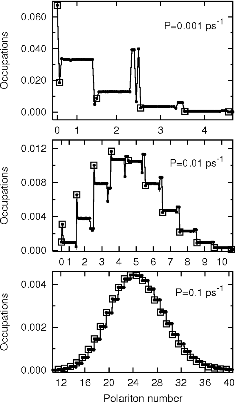
Figure 6: Occupations at three different pumping rates: low (upper panel), intermediate (polariton laser, central panel), and high pumping (lower panel). The detuning parameter is $\Delta=-3$ meV.

In what follows, in order to extend the analysis up to relatively high polariton numbers ($N_{pol}^{(max)}=600$), we will neglect the coherences. The number of variables reduces to $20N_{pol}^{(max)}-2$. For the occupations in the stationary limit, Eqs. (5) take the explicit form:

$$0 = \kappa\sum_{J}|\langle I|a|J\rangle|^{2}\rho_{JJ}-\kappa\rho_{II}\sum_{J}|\langle J|a|I\rangle|^{2}$$ (6)

$$+ P\sum_{N_{pol}(J)=N_{pol}(I)-1}\rho_{JJ}-P\rho_{II}N_{up}(I),$$

where $N_{up}(I)$ counts the number of states with polariton number $N_{pol}(I)+1$. We have $N_{up}(1)=17$, $N_{up}(I)=20$ for $1\leq N_{pol}(I)<N_{pol}^{(max)}$ and, finally, $N_{up}(I)=0$ for $N_{pol}(I)=N_{pol}^{(max)}$.

The set of homogeneous linear equations (6) should be complemented with the constraint,

$$\sum_{I}\rho_{II}=1,$$ (7)

which corresponds to the conservation of probability.

We show in Fig. 6 three regimes of pumping: low, intermediate, and large pumping rates, clearly differentiated by the patterns of occupations. In that figure, the $y$-axis corresponds to the occupations $\rho_{II}$, whereas in the $x$-axis the states are arranged in increasing order of the polariton number, $N_{pol}$. Recall that the first state is the vacuum with $N_{pol}=0$, then we have 17 states with $N_{pol}=1$, then 20 states with $N_{pol}=2$, etc. The ground state in each sector with fixed $N_{pol}$ is indicated by a square.

At low pumping rates, the mean polariton number, defined as $\langle N_{pol}\rangle=\sum_{I}\rho_{II}N_{pol}(I)$, is $\langle N_{pol}\rangle\approx 1$. The state with the highest occupation is the vacumm. The ground-state occupations in sectors with $N_{pol}>1$ are depressed. On the other hand, in the situation represented in the central panel of Fig. 6, $\langle N_{pol}\rangle$ is around four. The ground state occupations in sectors with $N_{pol}<\langle N_{pol}\rangle$ are enhanced with respect to the other states in the same sector. This is a kind of stimulated occupation of ground states. Finally, for large pumping rates the occupation in each sector with fixed $N_{pol}$ is nearly uniform. In the example shown in the lower panel of Fig. 6, $\langle N_{pol}\rangle$ is around 24. A broad bell of occupied states ranging from $N_{pol}\approx 12$ to around 40 is observed.

Once computed the stationary density matrix, one can estimate the photoluminescence response in the stationary state.

V The photoluminescence spectral function

In order to obtain the photoluminescence spectral function, $S(\omega)$, we follow the lines sketched in paper [Tejedor1, ]. $S(\omega)$ is defined in terms of the first-order correlation function of photons:

$$S(\omega)=\frac{1}{\pi}{\rm Re}\int_{0}^{\infty}{\rm d}\tau\exp(-i\omega\tau)\langle a^{\dagger}(t+\tau)a(t)\rangle.$$ (8)

This function is to be computed with the help of the Quantum Regression Theorem libroOC , which states that if we write:

$$\langle a^{\dagger}(t+\tau)a(t)\rangle=\sum_{I,J}\langle J|a^{\dagger}|I\rangle~{}g_{a,IJ},$$ (9)

the auxiliary operator:

$$g_{a,IJ}=\langle|J\rangle\langle I|(t+\tau)~{}a(t)\rangle,$$ (10)

satisfies with respect to $\tau$ the same master equation as the matrix elements $\rho_{IJ}$, with initial conditions:

$$\left.g_{a,IJ}\right|_{\tau=0}=\sum_{K}\langle I|a|K\rangle~{}\rho_{KJ}(t).$$ (11)

In the stationary limit, $t\to\infty$, we get $\rho_{KJ}(t)=\rho_{JJ}^{(\infty)}\delta_{KJ}$, and $g_{a,IJ}(\tau\to 0)=\langle I|a|J\rangle~{}\rho_{JJ}^{(\infty)}$. These initial conditions dictate that $g_{a,IJ}$ behaves in the same way as the “vertical” coherences, that is, $N_{pol}(I)=N_{pol}(J)-1$. Recall the equation for the vertical coherences, which may be obtained from Eq. (5):

$$\frac{\rm d}{{\rm d}\tau}g_{a,IJ} = (i\omega_{IJ}-\Gamma_{IJ})g_{a,IJ}$$ (12)

$$+ \kappa\sum_{K,M}\langle I|a|M\rangle g_{a,MK}\langle K|a^{\dagger}|J\rangle$$

$$- \frac{\kappa}{2}\sum_{K\neq I,M}\langle I|a^{\dagger}|M\rangle\langle M|a|K\rangle g_{a,KJ}$$

$$- \frac{\kappa}{2}\sum_{K,M\neq J}g_{a,IM}\langle M|a^{\dagger}|K\rangle\langle K|a|J\rangle,$$

where $\omega_{IJ}=(E_{J}-E_{I})/\hbar$, and

$$\Gamma_{IJ} = \frac{\kappa}{2}\sum_{K}\left\{\right|\langle K|a|I\rangle|^{2}+|\langle K|a|J\rangle|^{2}\}$$ (13)

$$+ \frac{P}{2}\{N_{up}(I)+N_{up}(J)\}.$$

The general solution of Eq. (12) is

$$g_{a,IJ}=\sum_{n}C_{n}e^{\lambda_{n}\tau}X_{IJ}^{(n)},$$ (14)

where $\lambda_{n}$ and $X_{IJ}^{(n)}$ are, respectively, the eigenvalues and eigenvectors of matrix $B_{IJ,MK}$, defined by the r.h.s. of Eq. (12), that is

$$\sum_{M,K}B_{IJ,MK}X_{MK}^{(n)}=\lambda_{n}X_{IJ}^{(n)}.$$ (15)

The coefficients $C_{n}$ are determined from the initial conditions:

$$\sum_{n}C_{n}X_{IJ}^{(n)}=\langle I|a|J\rangle\rho_{JJ}^{(\infty)}.$$ (16)

The explicit expression for $S(\omega)$ is the following:

$$S(\omega)=-\frac{1}{\pi}\sum_{I,J}\sum_{n}\frac{D^{(r)}_{IJ,n}\lambda_{n}^{(r)}+D^{(i)}_{IJ,n}(\lambda_{n}^{(i)}-\omega)}{(\lambda_{n}^{(r)})^{2}+(\lambda_{n}^{(i)}-\omega)^{2}}.$$ (17)

Where $D_{IJ,n}=\langle J|a^{\dagger}|I\rangle C_{n}X_{IJ}^{(n)}$, and the supraindexes $r$ and $i$ refer, respectively, to the real and imaginary parts of the magnitudes. The dimension of the matrix problems given by Eqs. (15) and (16) is $17+20\times 17+20\times 20\times(N_{pol}^{(max)}-2)$. When $N_{pol}^{(max)}=10$, for example, the dimension is 3557.

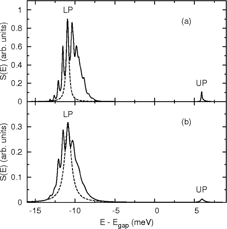
Figure 7: (a) PL spectral function computed from the exact expression, Eq. (17). (b) The spectral function computed from the approximate expression, Eq. (19). The detuning is $\Delta=-3$ meV, and the pumping rate, $P=0.006$ ps^-1.

We notice that there is an approximate expression for $S(\omega)$ which is based on the fact that $E_{J}-E_{I}\approx E_{gap}\approx 1500$ meV (for GaAs), whereas $\hbar\kappa$ and $\hbar P$ are smaller than 1 meV. In a first approximation, we take only the diagonal terms in Eq. (12), arriving to the following expression for the correlation function:

$$\left.\langle a^{\dagger}(t+\tau)a(t)\rangle\right|_{t\to\infty}$$

$$\approx\sum_{I,J}|\langle I|a|J\rangle|^{2}~{}\rho_{JJ}^{(\infty)}\exp(i\omega_{IJ}-\Gamma_{IJ})\tau,$$ (18)

from which it follows that

$$S(\omega)\approx\frac{1}{\pi}\sum_{I,J}\frac{|\langle I|a|J\rangle|^{2}\rho_{JJ}^{(\infty)}\Gamma_{IJ}}{\Gamma_{IJ}^{2}+(\omega_{IJ}-\omega)^{2}}.$$ (19)

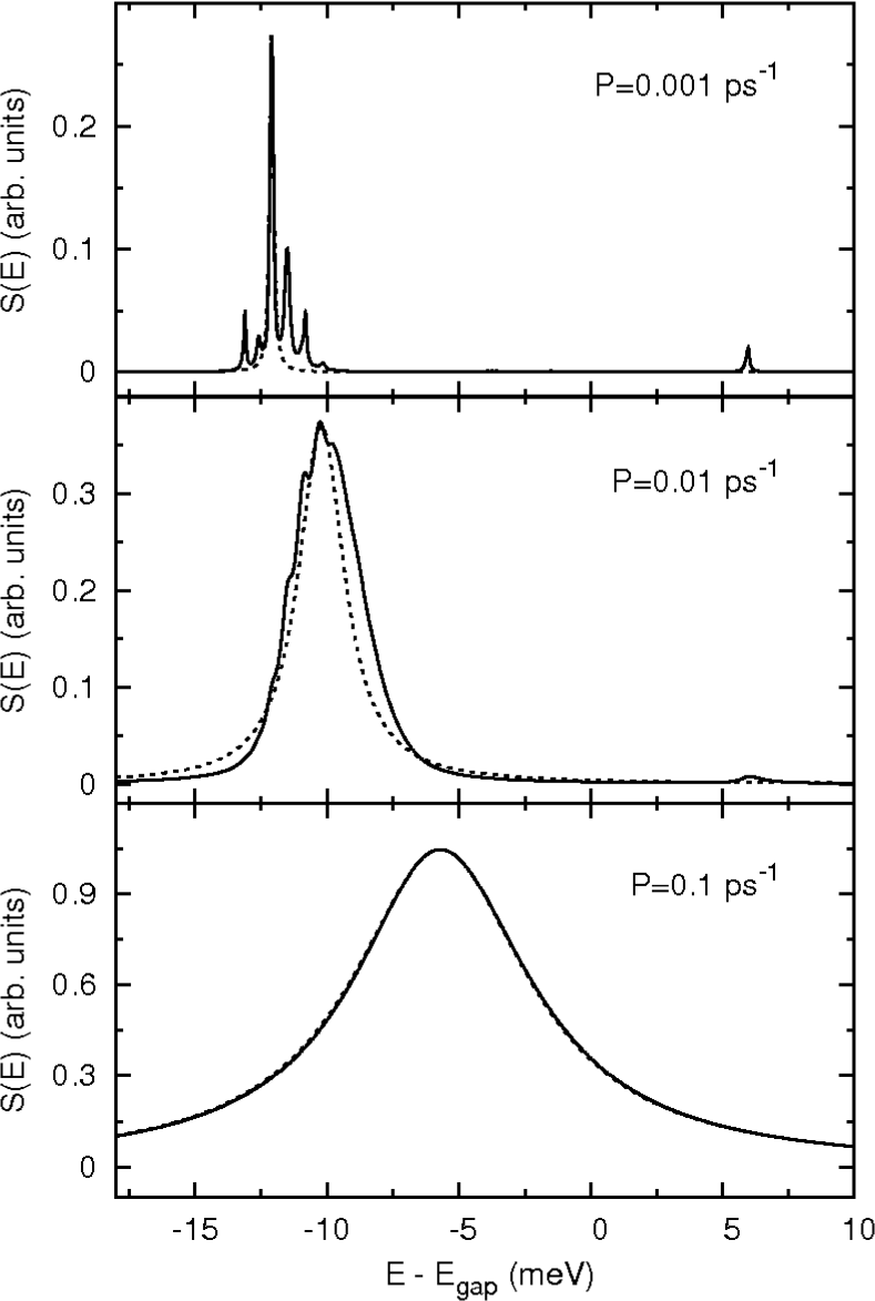
Figure 8: $S(E)$ and the Lorentzian fit (dashed line) to the LP peak for the three cases of Fig. 6.

The main advantage of expression (19) is the simplicity. The luminescence from state $J$ depends on the probability, $\rho_{JJ}$, that the state is occupied, and on the matrix elements $\langle I|a|J\rangle$ for emission of a photon. The widths $\Gamma_{IJ}$ have contributions from losses and pumping, the latter is also a source of decoherence.

Figure 9: Integrated intensity, position and linewidth of the lower polariton peak, coming from Eq. (19), as functions of the pumping rate. $\Delta=-3$ meV. For the additional lines in the center and bottom panels see explanation in the main text.

The nondiagonal terms in Eq. (12) can only slightly modify the position of resonances, given by $\omega_{IJ}$. They have a more appreciable effect on the widths. In Fig. 7, a comparison is made between the exact, Eq. (17), and approximate, Eq. (19), spectral functions. The parameters are such that the mean number of polaritons is $\langle N_{pol}\rangle=3.4$. The lower energy emission has contributions from different peaks. We notice, by the way, that multimode emission in the polariton lasing regime, which is a manifestation of its non-equilibrium nature, has been nicely demonstrated recently multimode . The strongest peak, which we take as the definition of the LP, is more sharper in the exact scheme. We will, nevertheless, use expression (19) in order to obtain the behaviour of the PL even for very strong pumping rates ($\langle N_{pol}\rangle\approx 500$), where an effective weak coupling regime is established.

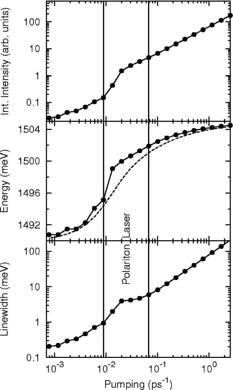
Figure 10: Same as Fig 9 for $\Delta=+5$ meV.

We fit the lower polariton peak to a Lorentzian (dashed line), from which the integrated intensity, peak position, and effective linewidth are extracted. In Fig. 8, we show $S(E)$ and the corresponding Lorentzian fit for the three cases illustrated in Fig. 6. The main characteristics of the polariton emission are apparent in the figure. That is, a blueshift of the emission, and an increase of the linewidth as the pumping rate is increased.

The upper panel of Fig. 9 shows the integrated intensity as a function of $P$ for a detuning $\Delta=-3$ meV. A threshold (change in the slope) at $P\approx 3\times 10^{-3}$ ps^-1 is observed, corresponding to stimulated ground-state occupations when the number of polaritons exceeds one. This is the “polariton laser” regime. At this threshold value, the peak position (center panel) begins a continuous blueshift towards the bare photon energy (1500-3=1497 meV), and the linewidth (bottom panel) starts increasing. In the “polariton laser” regime there is an interval where the linewidth saturates, and even decreases. This is better seen in the additional line (empty squares), computed from the exact equations, Eqs. (15-17). The decrease of the linewidth corresponds to maximum coherence, as will become evident below.

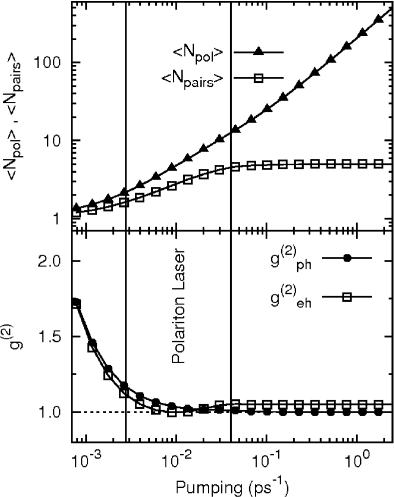
Figure 11: Upper panel: Mean number of polaritons and electron-hole pairs as a function of $P$. Lower panel: The second-order coherence functions at zero time delay for photons and electron-hole pairs. The detuning parameter is $\Delta=-3$ meV.

We draw an additional curve (dashed line) in Fig. 9, center panel, which refers to ground-state to ground-state transitions. This curve is constructed in the following way. For a given $P$, we find $\langle N_{pol}\rangle$. Then, the energy of the transition from the ground state of the system with polariton number equal to $\langle N_{pol}\rangle$ to the ground state of the system with polariton number equal to $\langle N_{pol}\rangle-1$ is found from Fig. 4(a). Comparison with this curve shows that the excited states, and states with polariton number higher than the mean value determine the position of the LP peak.

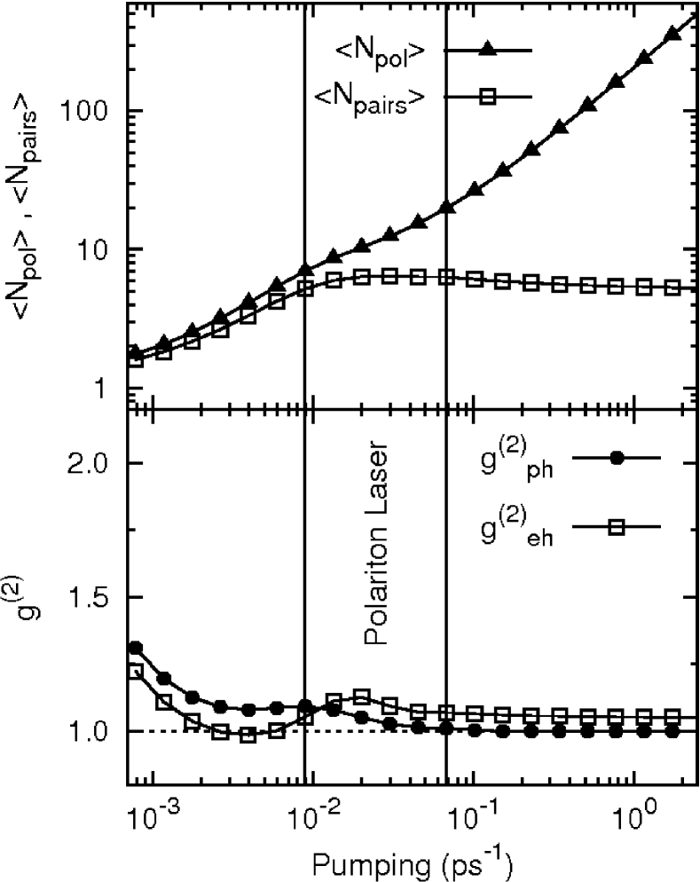
Figure 12: Same as Fig. 11 for $\Delta=+5$ meV.

The right border of the polariton laser regime is conventionally set to $P\approx 4\times 10^{-2}$ ps^-1 in this figure. It is characterized by a second change of slope in the intensity curve, and a renewed increase of linewidth. Let us notice that, in this quasiresonant case, the mean occupation of fermionic levels becomes near one half in the border, a fact that could be appreciated below. For strong pumping rates, we observe a tendency to saturation in the position of the peak (towards the photon energy), which indicates the emergence of a new regime characterized by an effective, weak photon-matter interaction.

In Fig. 10, we show results for positive detuning, $\Delta=+5$ meV, where the electron-hole contents of the wave functions are higher. At this level, they look very similar to those reported in Fig. 9. We can approximately fix the limits of the polariton laser regime as $9\times 10^{-3}<P<6\times 10^{-2}$ ps^-1. However, as it will become clear in the next section, the mean number of pairs is close to 5 near threshold, leading to a mean occupation of fermionic levels, $\langle N_{pairs}\rangle/10$, close to 1/2. This example shows that polariton lasing is not in antagonism with population inversion. Or, to set it in a different way, population inversion in these systems is not synonym of effectively weak pair-photon coupling. These results could be related to the small number of available states for fermions or the chosen values of the system parameters, but anyway they illustrate aspects of principle.

VI Second-order coherence functions

In Figs. 11 and 12, we show the mean number of polaritons, $\langle N_{pol}\rangle$, the mean number of pairs, $\langle N_{pairs}\rangle$, and the coherence properties of the photon and matter subsystems in the quasi-resonant and in the positive detuning case, respectively. We define the second-order coherence functions for photons and electron-hole pairs in terms of the one- and two-point correlation functions at zero time delay:

$$g^{(2)}_{ph}=\frac{\langle a^{\dagger}a^{\dagger}aa\rangle}{\langle a^{\dagger}a\rangle^{2}},$$ (20)

$$g^{(2)}_{eh}=\frac{\langle D^{\dagger}D^{\dagger}DD\rangle}{\langle D^{\dagger}D\rangle^{2}},$$ (21)

where $a$ is the photon annihilation operator, and $D=\sum_{i}h_{\bar{i}}e_{i}$ is the interband dipole operator.

The coherence functions evolve from values larger than two at low pumping rates to values near one (Poisson statistics, perfectly coherent state) immediately after the threshold. Notice that the electron-hole subsystem reaches coherence more rapidly than photons ($g^{(2)}_{eh}<g^{(2)}_{ph}$) possibly because of Coulomb interactions. For large values of $P$, we get $g^{(2)}_{eh}>g^{(2)}_{ph}\approx 1$. Notice also that, in the resonant case, there is a pumping rate for which both $g^{(2)}_{eh}$ and $g^{(2)}_{ph}$ are approximately equal to one. This is the point of maximum coherence, and corresponds to a minimum of the linewidth.

In the positive detuning case, the minimum of the linewidth is reached at the point where $g^{(2)}_{eh}$ has a local maximum. For low pumping rates, $\langle N_{pol}\rangle$ and $\langle N_{pairs}\rangle$ are very similar. They start differing precisely at the polariton lasing threshold, where the population of fermions is inverted.

VII Conclusions

In conclusion, we have computed the stationary density matrix, the photoluminescence spectral function, and the second-order coherence functions in a model polariton system describing a multi-level quantum dot strongly interacting with the lowest photon mode of a microcavity. The main features of polariton lasing, i.e. blueshift of the emission peak and increase of the linewidth as the pumping rate is rised, are reproduced by the model. Unexpected properties, such as the coexistence of polariton lasing and population inversion for positive detuning, are also manifested.

Our polariton model with a finite number of degrees of freedom, could be positioned in between the two-level system, studied in Ref. Tejedor1, , and the infinite degrees of freedom systems considered, for example, in Refs. previos, . Our model is simple enough to be numerically diagonalized but, at the same time, complex enough to capture many of the features of the infinite system. In this sense, our results could be qualitatively compared with the experiment reported in Ref. JBloch, , although the values of our model parameters are completely unrealistic.

Finally, we should stress that we are aware of the limitations of our model. We understand, for example, that $g^{(2)}$ does not rise further in the regime of strong pumping because the model does not include higher fermionic levels, which should become populated in this regime, that interact with the lowest polariton states, partially destroying coherence.

- (1) A. Kavokin and G. Malpuech, Cavity Polaritons (Elsevier, Amsterdam, 2003)
- (2) Y. Yamamoto, F. Tassone, H. Cao, Semiconductor Cavity Quantum Electrodynamics (Springer, New-York, 2000).
- (3) Hui Deng, D. Press, S. Gotzinger, G.S. Solomon, R. Hey, K.H. Ploog, and Y. Yamamoto, Phys. Rev. Lett. 97, 146402 (2006).
- (4) J. Kasprzak, M. Richard, S. Kundermann, A. Baas, P. Jeambrun, J.M.J. Keeling, F.M. Marchetti, M.H. Szymanska, R. Andre, J.L. Staehli, V. Savona, P.B. Littlewood, B. Deveaud, and LeSi Dang, Nature 443, 409 (2006).
- (5) D. Bajoni, P. Senellart, E. Wertz, I. Sagnes, A. Miard, A. Lemaitre, and J. Bloch, Phys. Rev. Lett. 100, 047401 (2008).
- (6) A. Imamoglu, R.J. Ram, S. Pau, and Y. Yamamoto, Phys. Rev. A 53, 4250 (1996).
- (7) H. Vinck, B.A. Rodriguez and A. Gonzalez, Physica E 35, 99 (2006).
- (8) H. Vinck-Posada, B.A. Rodriguez, P.S.S. Guimaraes, A. Cabo, and A. Gonzalez, Phys. Rev. Lett. 98, 167405 (2007).
- (9) C.A. Vera, A. Cabo, and A. Gonzalez, Phys. Rev. Lett. 102, 126404 (2009).
- (10) J.I. Perea, D. Porras, and C. Tejedor, Phys. Rev. B 70, 115304 (2004).
- (11) F.P. Laussy, E. del Valle, and C. Tejedor, Phys. Rev. Lett. 101, 083601 (2008).
- (12) J.I. Perea and C. Tejedor, Phys. Rev. B 72, 035303 (2005).
- (13) See, for example, P.R. Eastham, arxiv:0803.2997; Paolo Schwendimann and Antonio Quattropani, Phys. Rev. B 77, 085317 (2008); M. H. Szymanska, J. Keeling, P. B. Littlewood, Phys. Rev. B 75, 195331 (2007); T. D. Doan, Huy Thien Cao, D. B. Thoai, and H. Haug, Phys. Rev. B 74, 115316 (2006); M.H. Szymanska, J. Keeling, and P.B. Littlewood, Phys. Rev. Lett. 96, 230602 (2006); Fabrice P. Laussy, G. Malpuech, A. Kavokin, and P. Bigenwald, Phys. Rev. Lett. 93 (2004) 016402; D. Porras and C. Tejedor, Phys. Rev. B 67, 161310 (2003); D.M. Whittaker, Phys. Rev. Lett. 80, 4791 (1998).
- (14) J.M. Gerard, D. Barrier, J.Y. Marzin, R. Kuszelewicz, L. Manin, E. Costard, V. Thierry-Mieg, and T. Rivera, Appl. Phys. Lett. 69, 4 (1996).
- (15) H. Haug and S.W. Koch, Quantum theory of the optical and electronic properties of semiconductors (World Scientific, Singapore, 1990).
- (16) J. Kasprzak, R. Andre, Le Si Dang, I.A. Shelykh, A.V. Kavokin, Y.G. Rubo, K.V. Kavokin, and G. Malpuech, Phys. Rev. B 75, 045326 (2007).
- (17) R.H. Dicke, Phys. Rev. 93, 99 (1954).
- (18) P.R. Eastham and P.B. Littlewood, Phys. Rev. B 64, 235101 (2001).
- (19) Aji A. Anappara, S. De Liberato, A. Tredicucci, C. Ciuti, G. Biasol, L. Sorba, and F. Beltram, arXiv:0808.3720.
- (20) J.K. Cullum and R.A. Willoughby, Lanczos algorithms for large symmetric eigenvalue computations (Birkhauser, Boston, 1985).
- (21) F. Tassone, C. Piermarocchi, V. Savona, A. Quattropani, and P. Schwendimann, Phys. Rev. B 56 (1997) 7554; A.I. Tartakovskii, M. Emam-Ismail, R.M. Stevenson, M.S. Skolnick, V.N. Astratov, D.M. Whittaker, J.J. Baumberg, and J.S. Roberts, Phys. Rev. B 62 (2000) R2283; F. Tassone and Y. Yamamoto, Phys. Rev. B 59 (1999) 10830; T.D. Doan, H.T. Cao, D.B. Tran Thoai, and H. Haug, Phys. Rev. B 72 (2005) 085301.
- (22) M.O. Scully and S. Subairy, Quantum Optics (Cambridge University Press, Cambridge, 2001).
- (23) D.N. Krizhanovskii, K.G. Lagoudakis, M. Wouters, B. Pietka, R.A. Bradley, K. Guda, D.M. Whittaker, M.S. Skolnick, B. Deveaud-Pledran, M. Richard, R. Andre, and LeSi Dang, arXiv:0903.1570.