Total forces in the diffusion Monte Carlo method with nonlocal pseudopotentials

Abstract

We report exact expressions for atomic forces in the diffusion Monte Carlo (DMC) method when using nonlocal pseudopotentials. We present approximate schemes for estimating these expressions in both mixed and pure DMC calculations, including the pseudopotential Pulay term and the Pulay nodal term. Harmonic vibrational frequencies and equilibrium bond lengths are derived from the DMC forces and compared with those obtained from DMC potential energy curves. Results for four small molecules show that the equilibrium bond lengths obtained from our best force and energy calculations differ by less than 0.002 Å.

I Introduction

The diffusion Monte Carlo (DMC) method is the most accurate approach available for calculating total ground-state energies of large many-electron systems (Foulkes et al., 2001). Energy derivatives, and in particular atomic forces, are of great importance as they may be used to relax atomic structures and perform molecular dynamics simulations. It has, however, proven difficult to develop accurate and efficient ways of calculating atomic forces within the DMC method.

The DMC method involves using the imaginary-time Schrödinger equation to project away excited states of a many-electron wavefunction so that the ground-state wavefunction $\Phi$ remains. The fermionic symmetry is maintained by the fixed-node approximation (Anderson, 1976) which constrains the nodal surface of $\Phi$ (the hypersurface on which $\Phi$ is zero) to equal that of an antisymmetric trial wavefunction $\Psi_{\mathrm{T}}$. The standard DMC algorithm generates the “mixed” probability distribution $\Psi_{\mathrm{T}}\Phi$ which can be used to calculate unbiased expectation values (apart from the fixed-node error) of operators that commute with the Hamiltonian, $\hat{H}$. If, however, an operator does not commute with $\hat{H}$, the “pure” probability distribution $\Phi\Phi$ is required which can be generated within the DMC method using, for example, the future-walking algorithm (Barnett et al., 1991).

Within the Born-Oppenheimer approximation the atomic positions are treated as parameters rather than dynamical variables, and the total atomic force is defined as the negative energy gradient with respect to the atomic position. In the mixed and pure DMC methods, the total force estimators are constructed by taking the gradient of the (mixed and pure) DMC energy. As in other electronic structure methods, these estimators consist of contributions from the Hellmann-Feynman (HFT) force (Hellmann, 1937; Feynman, 1939) and from additional Pulay terms (Pulay, 1969; Badinski et al., 2008) which must be included to obtain unbiased estimates of the forces. Although the estimators for the HFT force have similar forms in the mixed and pure DMC methods, there are significant differences between the Pulay terms. The mixed DMC Pulay term involves the derivative of the unknown DMC wavefunction $\Phi$, which cannot be calculated straightforwardly. Reynolds et al. (Reynolds et al., 1986a, b) suggested using the derivative of $\Psi_{\mathrm{T}}$ instead and obtained a practical, although approximate, scheme for estimating the mixed DMC Pulay term. The pure DMC Pulay term involves an integral over the nodal surface (Schautz and Flad, 1999) which cannot be calculated in a standard DMC calculation. A practical but approximate scheme for estimating this nodal surface term has recently been developed (Badinski et al., 2008).

Although mixed DMC total forces have been investigated in studies of small molecules (Assaraf and Caffarel, 1999, 2000; Casalegno et al., 2003), the pure DMC nodal surface term (Chiesa et al., 2005; Badinski and Needs, 2007) has not been calculated for real systems. In a recent study of a model system without electron-electron interactions, however, the nodal term was found to be important (Badinski et al., 2008). Also, no previous study has directly compared the performance of the mixed and pure DMC forces for real systems.

It is well-known that the HFT estimator has an infinite variance when the bare Coulomb potential is used to describe the electron-nucleus interaction. Different routes have been proposed to address this problem. Assaraf et al. (Assaraf and Caffarel, 1999, 2000, 2003) added a term to the HFT force which has a zero mean value but greatly reduces the variance of the estimator. Chiesa et al. (Chiesa et al., 2005) developed a method to filter out the part of the electron density that gives rise to the infinite variance. Using soft pseudopotentials also eliminates the infinite variance problem (Badinski and Needs, 2007), and this method is used in the current work.

Pseudopotentials not only resolve the infinite variance issue when calculating forces, they also remove the chemically inert core electrons and their rapid spatial variations from the problem. This greatly reduces the computational cost of a DMC calculation which scales with the atomic number, $Z$, as $Z^{5.5}$. (Ceperley, 1986; Ma et al., 2005) However, the use of pseudopotentials introduces additional Pulay-like terms in the HFT force estimator (Badinski and Needs, 2007) which have been neglected in previous calculations. In this work we have included these pseudopotential Pulay terms.

We investigate the accuracy of the mixed and pure DMC force estimates for the H₂, SiH, GeH and SiH₄ molecules. Bond lengths and harmonic vibrational frequencies are obtained from the forces and are compared with those obtained from DMC energy calculations. These results are used to both evaluate the importance of the different Pulay terms and to compare the performance of the mixed and pure DMC force estimators.

This paper is organized as follows. In Sec. 2 we give exact and approximate expressions for the forces under different pseudopotential localization schemes. In Sec. 3 we describe our DMC calculations and in Sec. 4 we present and discuss the molecular bond lengths and vibrational frequencies obtained. We draw our conclusions in Sec. 5.

II Forces in the diffusion Monte Carlo method

We write the valence Hamiltonian for a many-electron system as

$$\hat{H}=\hat{H}_{\mathrm{loc}}+\hat{W},$$ (1)

where $\hat{H}_{\mathrm{loc}}$ consists of the kinetic energy, the Coulomb interaction between the electrons and the local pseudopotential, and $\hat{W}$ is the nonlocal pseudopotential operator. Two different pseudopotential localization approximation (PLA) schemes have been introduced to evaluate the nonlocal action of $\hat{W}$ on the DMC wavefunction, $\Phi$. In these schemes $\hat{H}$ is replaced by an effective Hamiltonian (Hurley and Christiansen, 1986; Casula, 2006),

$$\hat{H}_{A} = \hat{H}_{\mathrm{loc}}+\frac{\hat{W}\Psi_{\mathrm{T}}}{\Psi_{\mathrm{T}}},$$ (2)

$$\hat{H}_{B} = \hat{H}_{\mathrm{loc}}+\frac{\hat{W}^{+}\Psi_{\mathrm{T}}}{\Psi_{\mathrm{T}}}+\hat{W}^{-}.$$ (3)

The nonlocal pseudopotential operator $\hat{W}^{+}$ corresponds to all positive matrix elements $\left<\mathbf{r}^{\prime}\right|\hat{W}^{+}\left|\mathbf{r}^{\prime}\right>$, and $\hat{W}^{-}$ corresponds to all negative matrix elements (Casula, 2006), where $\mathbf{r}$ is the 3$N$-dimensional position vector for the $N$ electron system and $N$ is the total number of electrons. Following Ref. (Badinski and Needs, 2007), these two approximations are referred to as the full-PLA (FPLA) and semi-PLA (SPLA) when using $\hat{H}_{A}$ or $\hat{H}_{B}$, respectively. The corresponding fixed-node DMC ground-state wavefunctions are denoted by $\Phi_{A}$ and $\Phi_{B}$.

The DMC energy can be written in the form

$$E_{\mathrm{D}}=\frac{{\displaystyle{\int}\Phi\hat{H}\Psi\mathrm{d}V}}{{\displaystyle{\int}\Phi\Psi\mathrm{d}V}},$$ (4)

which includes the mixed DMC ($\Psi=\Psi_{\mathrm{T}}$) and pure DMC ($\Psi=\Phi)$ estimates of the energy. In all later expressions, $\Phi$ stands for either $\Phi_{A}$ or $\Phi_{B}$, and $\hat{H}$ for either $\hat{H}_{A}$ or $\hat{H}_{B}$. Although the mixed and pure estimates of $E_{\mathrm{D}}$ in Eq. (4) are equivalent for a given localization approximation, $E_{\mathrm{D}}$ may differ under the two localization schemes.

We now consider a general parameter $\lambda$, e.g., a nuclear coordinate, which is used to vary the Hamiltonian, and upon which both the nodal surface (via $\Psi_{\mathrm{T}}$) and the DMC wavefunction $\Phi$ depend. Taking the derivative of the DMC energy with respect to $\lambda$ gives

$$\frac{\mathrm{d}E_{\mathrm{D}}}{\mathrm{d}\lambda} = \frac{{\displaystyle{\int}\left[\Phi\hat{H}^{\prime}\Psi+\Phi\left(\hat{H}-E_{\mathrm{D}}\right)\Psi^{\prime}\right]\mathrm{d}V}}{{\displaystyle{\int}\Phi\Psi\,\mathrm{d}V}}$$ (5)

$$+\frac{{\displaystyle{\int}\left[\Phi^{\prime}\left(\hat{H}-E_{\mathrm{D}}\right)\Psi\right]\mathrm{d}V}}{{\displaystyle{\int}\Phi\Psi\,\mathrm{d}V}},$$

for both the mixed and pure DMC methods. We use the notation $\alpha^{\prime}=\frac{\mathrm{d}\alpha}{\mathrm{d}\lambda}$ where $\alpha$ can be a function or an operator. The first term in Eq. (5) is the HFT force (Hellmann, 1937; Feynman, 1939) and the others are Pulay terms (Pulay, 1969).

II.1 Mixed DMC forces

The total force in the mixed DMC method, $F_{\mathrm{mix}}^{\mathrm{tot}}$, is obtained by setting $\Psi=\Psi_{\mathrm{T}}$ in Eq. (5). After some rearrangements, we arrive at

$$F_{\mathrm{mix}}^{\mathrm{tot}}=F_{\mathrm{mix}}^{\mathrm{HFT}}+F_{\mathrm{mix}}^{\mathrm{P}}+F_{\mathrm{mix}}^{\mathrm{V}}+F_{\mathrm{mix}}^{\mathrm{N}},$$ (6)

with

$$F_{\mathrm{mix}}^{\mathrm{HFT}} = -\frac{{\displaystyle{\int}\Phi\Psi_{\mathrm{T}}\left(\frac{\hat{W}^{\prime}\Psi_{\mathrm{T}}}{\Psi_{\mathrm{T}}}\right)\mathrm{d}V}}{{\displaystyle{\int}\Phi\Psi_{\mathrm{T}}\,\mathrm{d}V}}-\frac{{\displaystyle{\int}\Phi\Psi_{\mathrm{T}}V_{\mathrm{loc}}^{\prime}\mathrm{d}V}}{{\displaystyle{\int}\Phi\Psi_{\mathrm{T}}\,\mathrm{d}V}}$$ (7)

$$+Z_{\alpha}\sum_{\beta\,(\beta\neq\alpha)}Z_{\beta}\frac{\mathbf{R}_{\alpha}-\mathbf{R}_{\beta}}{|\mathbf{R}_{\alpha}-\mathbf{R}_{\beta}|^{3}}$$

$$F_{\mathrm{mix}}^{\mathrm{P}} = -\frac{{\displaystyle{\int}\Phi\Psi_{\mathrm{T}}\left[\frac{\hat{W}\Psi_{\mathrm{T}}^{\prime}}{\Psi_{\mathrm{T}}}-\left(\frac{\hat{W}\Psi_{\mathrm{T}}}{\Psi_{\mathrm{T}}}\right)\frac{\Psi_{\mathrm{T}}^{\prime}}{\Psi_{\mathrm{T}}}\right]\mathrm{d}V}}{{\displaystyle{\int}\Phi\Psi_{\mathrm{T}}\,\mathrm{d}V}}$$ (8)

$$F_{\mathrm{mix}}^{\mathrm{V}} = -\frac{{\displaystyle{\int}\Phi\Psi_{\mathrm{T}}\left[\frac{\Phi^{\prime}}{\Phi}\frac{\left(\hat{H}-E_{\mathrm{D}}\right)\Psi_{\mathrm{T}}}{\Psi_{\mathrm{T}}}\right]\mathrm{d}V}}{{\displaystyle{\int}\Phi\Psi_{\mathrm{T}}\,\mathrm{d}V}}$$ (9)

$$F_{\mathrm{mix}}^{\mathrm{N}} = -\frac{{\displaystyle{\int}\Phi\Psi_{\mathrm{T}}\left[\frac{\left(\hat{H}-E_{\mathrm{D}}\right)\Psi_{\mathrm{T}}^{\prime}}{\Psi_{\mathrm{T}}}\right]\mathrm{d}V}}{{\displaystyle{\int}\Phi\Psi_{\mathrm{T}}\,\mathrm{d}V}}.$$ (10)

$F_{\mathrm{mix}}^{\mathrm{HFT}}$ is the mixed DMC HFT force and the other expressions are Pulay terms. The HFT force in Eq. (7) contains two contributions from the pseudopotential, one from its local part $V_{\mathrm{loc}}$ and one from its nonlocal part $\hat{W}$, and a third contribution from the nucleus-nucleus interaction. In this nucleus-nucleus interaction term, $\mathbf{R}_{\alpha}$ represents the $3$-dimensional position vector of the $\alpha$th nucleus, and $Z_{\alpha}$ is the associated charge. The three Pulay terms in Eqs. (8)-(10) are identified as follows: $F_{\mathrm{mix}}^{\mathrm{P}}$ results from the PLA and is therefore called the pseudopotential Pulay term, $F_{\mathrm{mix}}^{\mathrm{V}}$ is the volume term, and $F_{\mathrm{mix}}^{\mathrm{N}}$ is called the mixed DMC nodal term since it can be written as an integral over the nodal surface (Badinski et al., 2008). Note that all terms in Eqs. (7)-(10) take the same form under both localization schemes, the only difference is the distribution ($\Psi_{\mathrm{T}}\Phi_{A}$ or $\Psi_{\mathrm{T}}\Phi_{B}$) used to evaluate the expectation values. A simple way to understand this is to note that $\hat{H}$ always acts on the trial wavefunction $\Psi_{\mathrm{T}}$ and $\hat{H}_{A}\Psi_{\mathrm{T}}=\hat{H}_{B}\Psi_{\mathrm{T}}$.

In mixed DMC simulations, it is straightforward to evaluate the contributions to the force except for the volume term $F_{\mathrm{mix}}^{\mathrm{V}}$, because it depends on the derivative of the DMC wavefunction, $\Phi^{\prime}$. Since it is unclear how to evaluate $\Phi^{\prime}$ in mixed DMC calculations, we use the Reynolds’ approximation (Reynolds et al., 1986a, b),

$$\frac{\Phi^{\prime}}{\Phi}\simeq\frac{\Psi_{\mathrm{T}}^{\prime}}{\Psi_{\mathrm{T}}},$$ (11)

which is exact on the nodal surface (see Eqs. (4) and (16) of Ref. (Badinski et al., 2008)) but introduces an error of first order in ($\Psi_{\mathrm{T}}-\Phi$) away from the nodal surface.

II.2 Pure DMC forces

The total force in the pure DMC method, $F_{\mathrm{pure}}^{\mathrm{tot}}$, is obtained by setting $\Psi=\Phi$ in Eq. (5). After some manipulations, we obtain

$$F_{\mathrm{pure}}^{\mathrm{tot}}=F_{\mathrm{pure}}^{\mathrm{HFT}}+F_{\mathrm{pure}}^{\mathrm{P}}+F_{\mathrm{pure}}^{\mathrm{N}},$$ (12)

with

$$F_{\mathrm{pure}}^{\mathrm{HFT}} = \left\{\begin{array}[]{c}-\frac{{\displaystyle{\int}\Phi_{A}\Phi_{A}\left(\frac{\hat{W}^{\prime}\Psi_{\mathrm{T}}}{\Psi_{\mathrm{T}}}\right)\mathrm{d}V}}{{\displaystyle{\int}\Phi_{\mathrm{A}}\Phi_{\mathrm{A}}\,\mathrm{d}V}}\\ -\frac{{\displaystyle{\int}\Phi_{B}\Phi_{B}\left(\frac{(\hat{W}^{+})^{\prime}\Psi_{\mathrm{T}}}{\Psi_{\mathrm{T}}}+\frac{(\hat{W}^{-})^{\prime}\Phi_{\mathrm{B}}}{\Phi_{\mathrm{B}}}\right)\mathrm{d}V}}{{\displaystyle{\int}\Phi_{B}\Phi_{B}\,\mathrm{d}V}}\end{array}\right\}$$ (16)

$$-\frac{{\displaystyle{\int}\Phi\Phi V^{\prime}_{\mathrm{loc}}\mathrm{d}V}}{{\displaystyle{\int}\Phi\Phi\,\mathrm{d}V}}+Z_{\alpha}\sum_{\beta\,(\alpha\neq\beta)}Z_{\beta}\frac{\mathbf{R}_{\alpha}-\mathbf{R}_{\beta}}{|\mathbf{R}_{\alpha}-\mathbf{R}_{\beta}|^{3}}$$

$$F_{\mathrm{pure}}^{\mathrm{P}} = \left\{\begin{array}[]{c}-\frac{{\displaystyle{\int}\Phi_{A}\Phi_{A}\left[\frac{\hat{W}\Psi_{\mathrm{T}}^{\prime}}{\Psi_{\mathrm{T}}}-\left(\frac{\hat{W}\Psi_{\mathrm{T}}}{\Psi_{\mathrm{T}}}\right)\frac{\Psi_{\mathrm{T}}^{\prime}}{\Psi_{\mathrm{T}}}\right]\mathrm{d}V}}{{\displaystyle{\int}\Phi_{A}\Phi_{A}\,\mathrm{d}V}}\\ -\frac{{\displaystyle{\int}\Phi_{B}\Phi_{B}\left[\frac{\hat{W}^{+}\Psi_{\mathrm{T}}^{\prime}}{\Psi_{\mathrm{T}}}-\left(\frac{\hat{W}^{+}\Psi_{\mathrm{T}}}{\Psi_{\mathrm{T}}}\right)\frac{\Psi_{\mathrm{T}}^{\prime}}{\Psi_{\mathrm{T}}}\right]\mathrm{d}V}}{{\displaystyle{\int}\Phi_{B}\Phi_{B}\,\mathrm{d}V}}\end{array}\right.$$ (19)

$$F_{\mathrm{pure}}^{\mathrm{N}} = \frac{1}{2}\frac{{\displaystyle{\int}_{\Gamma}|\nabla_{\mathbf{r}}\Phi|\Phi^{\prime}\,\mathrm{d}S}}{{\displaystyle{\int}\Phi\Phi\mathrm{d}V}}.$$ (20)

$F_{\mathrm{pure}}^{\mathrm{HFT}}$ is the pure DMC HFT force, $F_{\mathrm{pure}}^{\mathrm{P}}$ is the pure DMC pseudopotential Pulay term, and the pure DMC nodal term $F_{\mathrm{pure}}^{\mathrm{N}}$ is an integral over the nodal surface $\Gamma$ (defined by $\Psi_{\mathrm{T}}=0$). Where terms appear in braces, the upper one refers to the FPLA and the lower to the SPLA. The form of the nodal term in Eq. (20) is independent of the localization scheme. The nodal term involves the gradient $\nabla_{\mathbf{r}}\Phi$ evaluated at the nodal surface $\Gamma$. Ref. (Badinski et al., 2008) shows that this gradient is defined as its limit when approaching the nodal surface from within a nodal pocket (where $\Phi$ is nonzero). The derivation of the nodal term from Eq. (5) can be found in Refs. (Schautz and Flad, 1999; Badinski et al., 2008).

Although the HFT force $F_{\mathrm{pure}}^{\mathrm{HFT}}$ under the FPLA can be calculated in the pure DMC method, it is not straightforward to evaluate the action of the nonlocal operator $(\hat{W}^{-})^{\prime}$ on the unknown DMC wavefunction $\Phi_{B}$ in $F_{\mathrm{pure}}^{\mathrm{HFT}}$ under the SPLA scheme. Therefore, the following localization approximation,

$$\frac{(\hat{W}^{-})^{\prime}\Phi_{B}}{\Phi_{B}}\simeq\frac{(\hat{W}^{-})^{\prime}\Psi_{\mathrm{T}}}{\Psi_{\mathrm{T}}},$$ (21)

is used in the evaluation of $F_{\mathrm{pure}}^{\mathrm{HFT}}$ under the SPLA scheme which introduces an error of first order in $(\Psi_{\mathrm{T}}-\Phi)$.

Another complication arises with the pure DMC nodal term $F_{\mathrm{pure}}^{\mathrm{N}}$ in Eq. (20) because it involves the evaluation of an integral over the nodal surface. It is unclear how to evaluate such an integral in a standard DMC simulation. The following relationship suggested in Ref. (Badinski et al., 2008),

$$F_{\mathrm{pure}}^{\mathrm{N}}=2\,F_{\mathrm{mix}}^{\mathrm{N}}+\mathcal{O}[(\Psi_{\mathrm{T}}-\Phi)^{2}],$$ (22)

allows the approximate evaluation of $F_{\mathrm{pure}}^{\mathrm{N}}$ as twice its mixed DMC counterpart while introducing an error of second order in $(\Psi_{\mathrm{T}}-\Phi)$. $F_{\mathrm{mix}}^{\mathrm{N}}$ may be evaluated in a standard DMC simulation using the volume integral representation of Eq. (10). Equation (22) is an application of the standard extrapolation technique (Foulkes et al., 2001), as in this case the variational estimate of the nodal term is zero (Badinski et al., 2008).

It is worth stating that the pseudopotential Pulay terms in both mixed and pure DMC simulations vanish when $\Psi_{\mathrm{T}}$ equals $\Phi$, which follows by inspection. Also, the mixed and pure DMC nodal terms vanish when the nodal surface of $\Psi_{\mathrm{T}}$ is exact. The proof of this statement is analogous to the one presented in Appendix C of Ref. (Badinski et al., 2008).

II.3 Total versus partial derivatives

Since the atomic force equals the negative total derivative of the DMC energy with respect to a nucleus position $\lambda$, all previous expressions involve total derivatives, in particular $\Psi_{\mathrm{T}}^{\prime}$. Calculating the total derivatives involves knowledge of how the wavefunction changes with $\lambda$. In the variational Monte Carlo (VMC) method, all parameters $\{c_{i}\}$ that describe the wavefunction $\Psi_{\mathrm{T}}$ can in principle be uniquely specified, e.g., by minimizing the variational energy. The specification of all $\{c_{i}\}$ parameters does not, however, uniquely determine the derivative of $\Psi_{\mathrm{T}}$ with respect to $\lambda$. In standard quantum chemistry methods, the derivatives of the $c_{i}$ with respect to $\lambda$ are typically obtained by second-order perturbation theory (Takada et al., 2004; Per, 2005). Unfortunately, such an approach is not straightforward in VMC and DMC methods.

In this work, we follow a different route and approximate all total derivatives by their partial derivatives, which introduces an error of first order in $(\Psi_{\mathrm{T}}-\Phi)$. We expect, however, this approximation to be rather accurate for the following reason: taking the total derivative of the DMC energy with respect to $\lambda$ gives

$$\frac{dE_{\mathrm{D}}}{d\lambda}=\frac{\partial E_{\mathrm{D}}}{\partial\lambda}+\sum_{i}\frac{\partial E_{\mathrm{D}}}{\partial c_{i}}\frac{dc_{i}}{d\lambda},$$ (23)

where the $c_{i}$ are the parameters in $\Psi_{\mathrm{T}}$ and the Hamiltonian. The sum in Eq. (23) stems from the implicit dependencies of the parameters $c_{i}$ on $\lambda$. This sum is neglected when all total derivatives are replaced with partial derivatives in all previous force expressions. Since the DMC energy is approximately minimized with respect to the $c_{i}$, we expect that the parameters $c_{i}$ have little effect on the DMC energy, i.e., $\frac{\partial E_{\mathrm{D}}}{\partial c_{i}}$ is small. Therefore, neglecting the sum in Eq. (23), or equivalently replacing all total derivatives with partials in our previous expressions, is expected to be a good approximation.

III Details of QMC calculations

	BL ($\mathrm{\AA}$)	Basis	$E_{\mathrm{HF}}$(Ha)	$E_{\mathrm{VMC}}$(Ha)	$E_{\mathrm{DMC}}$(Ha)	$E_{\mathrm{C}}$
H2	0.740	large	-1.13367	-1.17399(1)	-1.17452(1)	98.7 %
SiH	1.520	large	-4.26235	-4.36967(4)	-4.37719(2)	93.4 %
GeH	1.600	large	-4.24392	-4.34377(1)	-4.35143(2)	92.9 %
SiH4	1.480	large	-6.08924	-6.27247(3)	-6.27927(7)	96.4 %
SiH	1.520	small	-4.24689	-4.36563(6)	-4.37611(2)	91.9 %
GeH	1.600	small	-4.23275	-4.34156(2)	-4.34928(2)	93.4 %

Table 1: Hartree-Fock (HF), VMC and DMC energies (Ha) for four molecules. The first column specifies the bond length (BL) used, the second column gives the basis set, and the last column states the percentage of the DMC correlation energy retrieved within the VMC method, $E_{\mathrm{C}}$, as a measure of the accuracy of the Jastrow factor as defined in Ref. (Badinski and Needs, 2007). The error bars in $E_{\mathrm{C}}$ are smaller than 0.1 %.

We use a trial wavefunction of the standard single-determinant Slater-Jastrow(Foulkes et al., 2001) form. The orbitals forming the Slater-determinants are obtained from Hartree-Fock calculations using the gamess-us (Schmidt et al., 1993) code with atomic-centered Gaussian basis sets. For all molecules, we use a basis set of sextuple-$\zeta$ quality (without $f$ and $g$ functions but with four additional diffuse $p$ and $d$ functions). To study the influence of the basis set we also use a smaller Gaussian basis set for the SiH and GeH molecules with only five $s$ and two $p$-functions so that the trial wavefunctions $\Psi_{\mathrm{T}}$ and the nodal surface are less accurate. We refer to these two basis sets as large and small.

Table 1 shows that, when using the small instead of the large basis set, the DMC total energies increase by 1.01(3) mHa and 2.15(3) mHa for the SiH and GeH molecules, respectively.

We use Jastrow factors consisting of electron-electron, electron-nucleus, and electron-electron-nucleus terms, which are expanded in natural power series (Drummond et al., 2005). The wavefunction for H₂ has 87 variable parameters, while those for the other molecules have 157. The parameters in the Jastrow factors are optimized by first minimizing the variance of the local energy (Drummond and Needs, 2005), and subsequently minimizing the energy (Toulouse and Umrigar, 2007; Brown et al., 2007) while keeping the cutoff parameters of the Jastrow factor fixed (Drummond et al., 2005). We use Dirac-Fock averaged relativistic effective pseudopotentials (Trail and Needs, 2005a, b) which can be obtained online ($\tt{www.tcm.phy.cam.ac.uk/{\sim}mdt26/casino2\_pseudopotentials.html}$, ). The future-walking method (Barnett et al., 1991) is used to sample the pure estimates and all DMC calculations are performed using the casino code (Needs et al., 2008) version 2.1.

We use the analytic expressions derived in Ref. (Badinski and Needs, 2007) for evaluating the HFT force. The Pulay terms may also be evaluated using analytic expressions, but to make the code more easily adaptable to other trial wavefunction forms we use a finite-difference approach. This introduces an error which is linear in the infinitesimal nuclear displacement, $\Delta$. We find that $\Delta\approx 10^{-7}$ Å minimizes the resulting error in the Pulay terms which is about seven orders of magnitude smaller than the estimated values of the total forces.

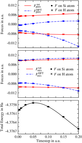
Figure 1: (Color online) Investigation of the timestep behaviour of DMC forces (a.u.) and DMC energies (Ha) for the SiH molecule when using the small basis set. Upper graph: the pure DMC forces $F_{\mathrm{pure}}^{\mathrm{tot}}$ and $F_{\mathrm{pure}}^{\mathrm{HFT}}$ as a function of the DMC timestep, circles indicate forces on the Si atom and crosses indicate forces on the H atom. A quadratic form is fitted to these forces. The standard errors of these forces are indicated unless they are smaller than the line width of the fitted functions. Middle graph: the same information as the upper graph for mixed DMC calculations. Lower graph: the DMC energy as a function of timestep for comparison, a cubic form is fitted to the energies.

DMC calculations suffer from systematic errors arising from the short-time approximation to the Green’s function, which we have carefully investigated. We find that the forces calculated with DMC timesteps of 0.01 and 0.005 a.u. agree with forces obtained from extrapolations to zero timestep within one standard error of less than 0.0005 a.u. Figure 1 shows such an investigation for the SiH molecule using the small basis set where the forces acting on the Si and H atoms are plotted as a function of timestep. We therefore use a timestep of 0.005 a.u. for all our DMC calculations, to avoid the necessity for repeated extrapolation to zero timestep. It is worth noting that, for the systems studied here, the timestep errors in the HFT and Pulay forces tend to cancel one another. This can be seen for the SiH molecule in Figure 1 when comparing the solid lines (total forces) with the dashed lines (HFT forces).

Figure 2: Dependence of the future-walking pure DMC HFT force estimates (a.u.) on the future-walking projection time (a.u.). Upper right graph: the HFT force on the Si atom for the SiH molecule as calculated within the mixed DMC and future-walking pure DMC method for different bond lengths using the small basis set. A Morse potential is fitted to these forces. Upper left graph: future-walking pure DMC forces calculated for different bond lengths plotted against the future-walking projection time. The mixed DMC force corresponds to zero future-walking projection time. Lower graphs: the same information as the upper graphs for the large basis set. When using the small or large basis set, we see that the future-walking projection time of 10 a.u. is long enough to obtain accurate pure DMC estimates.

For the future-walking pure DMC estimates to be accurate, an infinite future-walking projection time is in principle required. However, we found a projection time of 10 a.u. to be sufficient in our calculations as no significant changes in the estimates were found when using longer projection times. For example, Figure 2 shows the convergence of the pure HFT forces with respect to the projection time for the SiH molecule and both basis sets.

Form	Basis	$a^{E}$	$a_{\mathrm{mix}}^{F_{\mathrm{tot}}}$	$a_{\mathrm{pure}}^{F\mathrm{{}_{tot}}}$	$\omega^{E}$	$\omega_{\mathrm{mix}}^{F_{\mathrm{tot}}}$	$\omega_{\mathrm{pure}}^{F_{\mathrm{tot}}}$
P(3/2)	small	1.5242(7)	1.5138(1)	1.5259(8)	2000(18)	2096(4)	2050(14)
P(4/3)	small	1.5238(7)	1.5138(1)	1.5261(7)	1983(55)	2095(5)	2018(28)
Morse	small	1.5242(6)	1.5141(1)	1.5259(6)	1992(12)	2084(2)	2045(11)
P(3/2)	large	1.5195(8)	1.5105(2)	1.5175(11)	2069(18)	2089(4)	2061(18)
P(4/3)	large	1.5194(8)	1.5107(2)	1.5177(11)	2104(56)	2078(6)	2046(38)
Morse	large	1.5195(7)	1.5107(1)	1.5173(9)	2049(13)	2080(2)	2052(11)
Expt.		1.520	1.520	1.520	2042	2042	2042

Table 2: Bond lengths, $a$ ($\mathrm{\AA}$), and harmonic vibrational frequencies, $\omega$ (cm^-1), for the SiH molecule derived from different functional forms previously fitted to the DMC energies and forces. Three fitting forms are used as indicated in the first column, P(3/2) indicates that a cubic polynomial is fitted to the energies and a quadratic one to the forces, and similarly for P(4/3), and Morse indicates that a Morse potential is fitted to the energy and its derivative to the forces. The results are compared with the experimental values taken from Ref. (National Institute of Standards and Technology, $\tt{www.nist.gov}$, ).

To determine the equilibrium bond lengths, we calculate the forces at 0 %, $\pm$1.5 %, $\pm$3 %, and $\pm$4.5 % around the experimental bond lengths. We then fit the derivative of the Morse potential (Morse, 1929) with three free parameters to our force data and locate the zero-force geometry and the harmonic vibrational frequency. For all molecules, we compare results derived from the Morse potential with those obtained from quadratic and cubic fitting forms. We find that the influence of the different fitting forms on the derived bond lengths and frequencies is much less than one standard error except for a few cases when the forces are obtained from the mixed DMC total force estimator. There, the statistical error is much reduced and the influence of the fitting form on the derived bond lengths and frequencies is sometimes as large as two standard errors. Table 2, for example, presents results obtained from the different fitting forms as calculated for the SiH molecule with both basis sets. It is not obvious which fitting form is best suited to describe our fitted data. However, the Morse potential gives the smallest statistical error bars for all derived bond lengths and frequencies, which suggests that the Morse potential may indeed give the best description of our data. We also obtain bond lengths and frequencies from a Morse potential fitted to the calculated DMC energies.

The statistical error bars in the calculated bond lengths and frequencies are determined using a statistical method. For convenience, the DMC forces and energies evaluated at the seven different bond lengths are called a set of data. For each set of data, statistical noise is added where the noise is obtained from a Gaussian distribution with a variance specified by one standard error of the DMC force and energy estimates. 10⁵ different sets of data are generated in this manner and a Morse potential is fitted to these sets. The bond lengths and frequencies are obtained for all sets, they are averaged, and their statistical error bars are determined. Throughout this work, we use the convention that one standard error corresponds to a one-sigma confidence interval.

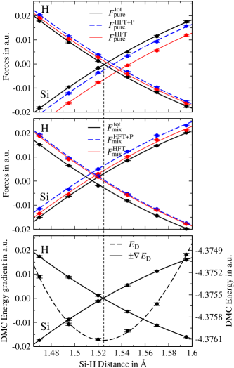
Figure 3: (Color online) Upper graph: three different estimates of the pure DMC forces, $F_{\mathrm{pure}}^{\mathrm{HFT}}$, $F_{\mathrm{pure}}^{\mathrm{HFT+P}}$ and $F_{\mathrm{pure}}^{\mathrm{tot}}$, for the Si and H atoms of the SiH molecule evaluated at different bond lengths. These estimates are defined in Eqs. (12)-(22) and are calculated with the small basis set. The Morse potential is fitted to the forces. Middle graph: the same information as for the upper graph with the three estimates, $F_{\mathrm{mix}}^{\mathrm{HFT}}$, $F_{\mathrm{mix}}^{\mathrm{HFT+P}}$ and $F_{\mathrm{mix}}^{\mathrm{tot}}$, calculated within the mixed DMC method. These estimates are defined in Eqs. (6)-(11). Lower graph: the DMC energy at different bond lengths, a Morse potential fitted to the DMC energies and the derivative of the Morse potential corresponding to the forces on the Si and H atoms. To guide the reader, the dotted vertical line corresponds to the zero-force geometry obtained from the fitted DMC energy curve.

For the SiH molecule, Figure 3 shows different DMC force estimates defined in Eqs. (6)-(22) and evaluated at different bond lengths. For reference, this figure also shows the DMC energies which are simultaneously calculated with the forces. A Morse potential fitted to the energies is also plotted together with its gradient. The dotted vertical line indicates the zero-force geometry obtained from the DMC energy curve. This figure shows that the geometry obtained from the minimum of the potential energy curve agrees well with the zero-force geometry obtained from the pure DMC total force estimates.

Since we investigate molecules containing H atoms and a heavier atom, one could obtain equilibrium bond lengths and vibrational frequencies from the forces on the H atoms alone. However, to test the force estimators on heavier atoms directly, we report bond lengths and frequencies obtained using both the zero-force condition on the H atom and on the heavier atoms. For SiH₄, the estimates of the forces on the Si atom should be zero by symmetry and this condition is satisfied within a standard error of less than 0.001 a.u. Also, the symmetries of the H₂ and SiH₄ molecules imply that the force on each H atom should have the same magnitude. Since we found this to hold within statistical errors, we average symmetry-related components to further reduce the statistical error bar.

IV Results

IV.1 Definitions

We define the errors in quantities such as bond lengths and frequencies as the differences between the values obtained from the forces and from the energies,

$$\Delta y_{\mathrm{method}}^{F}=y_{\mathrm{method}}^{F}-y^{E},$$ (24)

where $y$ is the bond length $a$ or vibrational frequency $\omega$, and the “method” can be mixed or pure DMC. $E$ indicates the DMC energy and $F$ stands for the different force estimators: HFT (the HFT estimator), HFT+P (with the pseudopotential Pulay estimator) and $F_{\mathrm{tot}}$, in the mixed DMC method as defined in Eqs. (6)-(11), and in the pure DMC method as defined in Eqs. (12)-(22).

In mixed DMC calculations, the error $\Delta y$ may arise from the Reynolds’ approximation of Eq. (11) and from replacing all total derivatives with partial derivatives. Both approximations introduce an error of first order in $(\Psi_{\mathrm{T}}-\Phi)$. In pure DMC calculations, the error $\Delta y$ may arise from the approximate nodal term in Eq. (22) and from replacing the total with partial derivatives. The latter approximation introduces an error of first order in ($\Psi_{\mathrm{T}}-\Phi$), whereas the approximate form of the nodal term introduces an error of second order.

IV.2 Bond lengths

	$a_{\mathrm{expt}}$	$a^{E}$	$a_{\mathrm{mix}}^{F^{\mathrm{tot}}}(1)$	$a_{\mathrm{pure}}^{F^{\mathrm{tot}}}(1)$	$a_{\mathrm{mix}}^{F^{\mathrm{tot}}}(2)$	$a_{\mathrm{pure}}^{F^{\mathrm{tot}}}(2)$
H2	0.741	0.7416(2)	0.74090(3)	0.7411(2)
SiH	1.520	1.5195(7)	1.5123(1)	1.5179(8)	1.5107(1)	1.5173(9)
GeH	1.589	1.6012(8)	1.5913(1)	1.5993(9)	1.5901(1)	1.5992(10)
SiH4	1.480	1.4740(4)	1.46970(9)	1.4728(10)

Table 3: Equilibrium bond lengths ($\mathrm{\AA}$) for four molecules calculated from mixed and pure DMC forces on each atom. The first column gives the experimental bond lengths from Ref. (National Institute of Standards and Technology, $\tt{www.nist.gov}$, ), the second column shows values obtained from the DMC energy curves, and the other columns give bond lengths obtained from the zero-force condition for the mixed and pure DMC total force estimators as defined in Eqs. (6) and (12). We specify bond lengths obtained from forces on the H atoms by (1) and on the non-H atoms by (2).

	Basis	$a^{E}$	$\,\,\,\Delta a_{\mathrm{mix}}^{\mathrm{HFT}}(1)$	$\,\,\,\Delta a_{\mathrm{mix}}^{\mathrm{HFT+P}}(1)$	$\,\,\,\Delta a_{\mathrm{mix}}^{F_{\mathrm{tot}}}(1)$	$\,\,\,\Delta a_{\mathrm{pure}}^{\mathrm{HFT}}(1)$	$\,\,\,\Delta a_{\mathrm{pure}}^{\mathrm{HFT+P}}(1)$	$\,\,\,\Delta a_{\mathrm{pure}}^{F_{\mathrm{tot}}}(1)$
H2	large	0.7416(2)	-0.0057(2)	-0.0057(2)	-0.0007(2)	-0.0002(2)	-0.0003(2)	-0.0004(3)
SiH	large	1.5195(7)	-0.0098(8)	-0.0091(8)	-0.0072(7)	-0.0006(10)	0.0007(10)	-0.0016(11)
GeH	large	1.6012(8)	-0.0138(9)	-0.0141(9)	-0.0099(8)	-0.0012(11)	-0.0018(11)	-0.0019(12)
SiH4	large	1.4740(4)	-0.0055(6)	-0.0056(6)	-0.0043(4)	-0.0005(8)	-0.0007(8)	-0.0012(11)
SiH	small	1.5242(6)	0.0006(7)	0.0023(7)	-0.0091(6)	0.0052(8)	0.0086(8)	0.0004(9)
GeH	small	1.5991(7)	-0.0059(7)	-0.0058(7)	-0.0060(7)	0.0024(10)	0.0028(10)	-0.0010(11)
	Basis	$a^{E}$	$\,\,\,\Delta a_{\mathrm{mix}}^{\mathrm{HFT}}(2)$	$\,\,\,\Delta a_{\mathrm{mix}}^{\mathrm{HFT+P}}(2)$	$\,\,\,\Delta a_{\mathrm{mix}}^{F_{\mathrm{tot}}}(2)$	$\,\,\,\Delta a_{\mathrm{pure}}^{\mathrm{HFT}}(2)$	$\,\,\,\Delta a_{\mathrm{pure}}^{\mathrm{HFT+P}}(2)$	$\,\,\,\Delta a_{\mathrm{pure}}^{F_{\mathrm{tot}}}(2)$
SiH	large	1.5195(7)	-0.0283(8)	-0.0279(8)	-0.0088(8)	-0.0032(10)	-0.0023(10)	-0.0022(11)
GeH	large	1.6012(8)	-0.0208(10)	-0.0200(10)	-0.0111(8)	-0.0044(12)	-0.0026(12)	-0.0020(13)
SiH	small	1.5242(6)	-0.0142(7)	-0.0207(7)	-0.0101(7)	0.0233(8)	0.0090(8)	0.0016(9)
GeH	small	1.5991(7)	-0.0220(8)	-0.0206(8)	-0.0085(7)	-0.0027(10)	0.0001(10)	-0.0023(12)

Table 4: Differences $\Delta a$ in the equilibrium bond lengths ($\mathrm{\AA}$) derived from the DMC forces and from the DMC energies. $\Delta a$ is defined by Eq. (24). The first column specifies the basis set used, the second column gives bond lengths obtained from the DMC energy curves, and the other columns give bond lengths obtained from the zero-force condition for the three different estimators, $F^{\mathrm{HFT}}$, $F^{\mathrm{HFT+P}}$, and $F^{\mathrm{tot}}$, in the mixed and pure DMC methods, defined in Eqs. (6)-(22). We specify bond lengths obtained from forces on the H atoms by (1) and on the non-H atoms by (2).

Table 3 presents equilibrium bond lengths calculated with the mixed and pure DMC total force estimators for four molecules using the FPLA. Table 4 gives further details of the different contributions to the total forces and presents the difference, $\Delta a$, of the bond lengths derived from the forces and from the energies, as defined in Eq. (24).

We begin by discussing pure DMC results with the large basis set. The HFT estimates $F_{\mathrm{pure}}^{\mathrm{HFT}}$ from forces on the H atoms give very accurate bond lengths (upper part of Table 4). As shown in the third last column of Table 4, the errors $\Delta a_{\mathrm{pure}}^{\mathrm{HFT}}(1)$ in the bond lengths derived from the forces on the H atoms are not much larger than one standard error of 0.001 Å. The bond lengths from the HFT forces calculated on the non-H atoms (lower part of Table 4) are not as accurate. Adding the pseudopotential Pulay term to the HFT forces, $F_{\mathrm{pure}}^{\mathrm{HFT+P}}$, has a very small effect on the bond lengths derived from the forces on the H atoms, as shown in the penultimate column of Table 4. For forces acting on the non-H atoms, however, adding the pseudopotential Pulay term improves the bond lengths slightly. The nodal terms are very small and do not significantly change the bond lengths obtained in the large basis set pure DMC calculations. The error bars on $\Delta a_{\mathrm{pure}}^{F_{\mathrm{tot}}}$ are dominated by the contribution from the HFT force, so that including the pseudopotential Pulay and nodal terms does not increase the noise much.

Table 4 shows that both the pseudopotential Pulay and nodal terms become more important for SiH and GeH when using the small basis set. The bond lengths from the HFT forces on both the H and Si atoms are significantly worse than for the large basis set. However, when the pseudopotential Pulay and nodal terms are included the bond lengths are not significantly worse than for the large basis set.

When comparing the mixed and pure DMC total force estimates, we find from Table 3 that the statistical errors in all bond lengths obtained from the mixed DMC forces are about a factor ten smaller. This is because the pure DMC estimator used here does not satisfy a zero-variance condition. The absolute deviation in all bond lengths derived from the mixed DMC total forces and from the energies is on average 0.0076(2) Å. In a similar comparison, the pure DMC total forces give bond lengths with a much smaller absolute average deviation of 0.0015(4) Å. Although adding the Pulay terms to the mixed DMC HFT force may improve the bond lengths by up to 17 standard errors in our results, all pure DMC forces (with and without Pulay terms) generally give more accurate bond lengths than the best mixed DMC total force estimates. This difference in accuracy can be understood by recalling that the error introduced in the mixed DMC force estimates is of first order in ($\Psi_{\mathrm{T}}-\Phi$) whereas the error in the pure DMC force estimates is only of second order. The additional first order error from replacing the total derivatives by partial derivatives appears to be small.

The differences between the DMC bond lengths (from either the DMC energy or the pure DMC forces) and experimental data in Table 3 are somewhat larger than the difference between the bond lengths from the DMC energies and forces. This difference is largest for GeH (0.010(1)-0.012(1) Å), followed by SiH₄ (0.006(0)-0.007(1) Å) and SiH (0.001(1)-0.003(1) Å) and is negligible for H₂. These bond length deviations from experiment must largely arise from a combination of the fixed-node approximation, the FPLA scheme, which slightly alters the pure DMC ground-state distribution, and the pseudopotentials. The fixed-node approximation could be improved by using more accurate trial wavefunctions. It is more difficult to develop better pseudopotentials, although including core-polarization potentials on the Si and Ge atoms may also improve the results (Shirley and Martin, 1993; Lee and Needs, 2003; Maezono et al., 2003).

IV.3 Vibrational Frequencies

	$\omega_{\mathrm{expt}}$	$\omega^{E}$	$\omega_{\mathrm{mix}}^{F_{\mathrm{tot}}}(1)$	$\omega_{\mathrm{pure}}^{F_{\mathrm{tot}}}(1)$	$\omega_{\mathrm{mix}}^{F_{\mathrm{tot}}}(2)$	$\omega_{\mathrm{pure}}^{F_{\mathrm{tot}}}(2)$
H2	4401	4420(16)	4441(2)	4403(15)
SiH	2042	2049(14)	2075(2)	2041(11)	2080(2)	2052(12)
GeH	1908(35)	1907(14)	1944(1)	1909(12)	1949(2)	1904(13)
SiH4	2187	2288(11)	2324(2)	2299(29)

Table 5: Harmonic vibrational frequencies (cm^-1) calculated within the mixed and pure DMC methods. The abbreviations are analogous to those in Table 3.

	Basis	$\omega^{E}$	$\Delta\omega_{\mathrm{mix}}^{\mathrm{HFT}}(1)$	$\Delta\omega_{\mathrm{mix}}^{\mathrm{HFT+P}}(1)$	$\Delta\omega_{\mathrm{mix}}^{F_{\mathrm{tot}}}(1)$	$\Delta\omega_{\mathrm{pure}}^{\mathrm{HFT}}(1)$	$\Delta\omega_{\mathrm{pure}}^{\mathrm{HFT+P}}(1)$	$\Delta\omega_{\mathrm{pure}}^{F_{\mathrm{tot}}}(1)$
H2	large	4420(16)	128(18)	128(18)	21(16)	-10(19)	-10(19)	-16(22)
SiH	large	2049(14)	68(15)	70(15)	26(13)	-10(16)	-7(16)	-7(18)
GeH	large	1907(14)	87(15)	89(15)	37(14)	1(16)	4(16)	2(18)
SiH4	large	2288(11)	71(16)	74(15)	36(11)	25(23)	30(23)	11(31)
SiH	small	1992(12)	71(13)	72(13)	81(12)	16(14)	19(15)	46(16)
GeH	small	1905(10)	74(11)	74(11)	29(10)	-25(13)	-25(13)	0(15)
	Basis	$\omega^{E}$	$\Delta\omega_{\mathrm{mix}}^{\mathrm{HFT}}(2)$	$\Delta a_{\mathrm{mix}}^{\mathrm{HFT+P}}(2)$	$\Delta a_{\mathrm{mix}}^{F_{\mathrm{tot}}}(2)$	$\Delta a_{\mathrm{pure}}^{\mathrm{HFT}}(2)$	$\Delta a_{\mathrm{pure}}^{\mathrm{HFT+P}}(2)$	$\Delta a_{\mathrm{pure}}^{F_{\mathrm{tot}}}(2)$
SiH	large	2049(14)	103(16)	100(17)	31(14)	14(16)	1(17)	3(18)
GeH	large	1907(14)	73(16)	68(16)	41(14)	2(17)	-10(17)	-4(19)
SiH	small	1992(12)	104(13)	129(13)	92(12)	-23(17)	27(15)	53(16)
GeH	small	1905(10)	86(12)	85(12)	38(10)	23(14)	17(14)	20(16)

Table 6: Difference $\Delta\omega$ in the harmonic vibrational frequencies (cm^-1) derived from the DMC forces and energies. The difference $\Delta\omega$ is defined by Eq. (24). The abbreviations are analogous to those in Table 4.

Table 5 presents harmonic vibrational frequencies calculated with the mixed and pure DMC total force estimators. Table 6 gives details of the different contributions to the total forces and presents the differences, $\Delta\omega$, of the frequencies derived from the forces and from the energies, as defined in Eq. (24).

Table 6 shows that for all pure DMC force estimators the difference in the vibrational frequencies derived from the forces and the energies is comparable to or less than one standard error of about $20\,\mathrm{cm}^{-1}$ with the exception of SiH. The effect of the pseudopotential Pulay and nodal terms on the pure DMC frequencies is small. This may also be seen qualitatively in Figure 3, where adding the Pulay terms mostly shifts the forces at different bond lengths by similar amounts.

As in the discussion of bond lengths, we find that the mixed DMC total forces give less accurate frequencies than the pure DMC forces. The absolute difference between frequencies derived from the mixed DMC total forces and from the energies is on average 43(4) cm^-1 compared to 16(6) cm^-1 when the frequencies are derived from pure DMC total forces. Although adding the Pulay terms to the mixed DMC HFT force may improve the frequencies by up to ten standard errors in our results, all pure DMC force estimates (with and without Pulay terms) still give more accurate frequencies than the best mixed DMC total force estimates.

IV.4 Comparison of the FPLA and SPLA schemes

	PLA	$a^{E}$	$\Delta a_{\mathrm{mix}}^{\mathrm{HFT}}(1)$	$\Delta a_{\mathrm{mix}}^{\mathrm{HFT+P}}(1)$	$\Delta a_{\mathrm{mix}}^{F_{\mathrm{tot}}}(1)$	$\Delta a_{\mathrm{pure}}^{\mathrm{HFT}}(1)$	$\Delta a_{\mathrm{pure}}^{\mathrm{HFT+P}}(1)$	$\Delta a_{\mathrm{pure}}^{F_{\mathrm{tot}}}(1)$
SiH	FPLA	1.5195(7)	-0.0098(8)	-0.0091(8)	-0.0072(7)	-0.0006(10)	0.0007(10)	-0.0016(11)
	SPLA	1.5210(8)	-0.0113(9)	-0.0110(9)	-0.0086(8)	-0.0024(10)	-0.0019(10)	-0.0034(11)
GeH	FPLA	1.6012(8)	-0.0138(9)	-0.0141(9)	-0.0099(8)	-0.0012(11)	-0.0018(11)	-0.0019(12)
	SPLA	1.5995(9)	-0.0129(10)	-0.0128(10)	-0.0073(9)	-0.0004(11)	-0.0004(11)	-0.0039(13)
	PLA	$a^{E}$	$\Delta a_{\mathrm{mix}}^{\mathrm{HFT}}(2)$	$\Delta a_{\mathrm{mix}}^{\mathrm{HFT+P}}(2)$	$\Delta a_{\mathrm{mix}}^{F_{\mathrm{tot}}}(2)$	$\Delta a_{\mathrm{pure}}^{\mathrm{HFT}}(2)$	$\Delta a_{\mathrm{pure}}^{\mathrm{HFT+P}}(2)$	$\Delta a_{\mathrm{pure}}^{F_{\mathrm{tot}}}(2)$
SiH	FPLA	1.5195(7)	-0.0283(8)	-0.0279(8)	-0.0088(8)	-0.0032(10)	-0.0023(10)	-0.0022(11)
	SPLA	1.5210(8)	-0.0303(9)	-0.0289(9)	-0.0098(8)	-0.0055(10)	-0.0026(10)	-0.0034(12)
GeH	FPLA	1.6012(8)	-0.0208(10)	-0.0200(10)	-0.0111(8)	-0.0044(12)	-0.0026(12)	-0.0020(13)
	SPLA	1.5995(9)	-0.0157(10)	-0.0148(10)	-0.0084(9)	-0.0060(12)	-0.0042(12)	-0.0033(15)

Table 7: Difference $\Delta a$ in the equilibrium bond lengths ($\mathrm{\AA}$) derived from the DMC forces and energies for SiH and GeH. The FPLA and SPLA localization approximations are used as indicated in the first column. All other abbreviations are the same as in Table 4.

	PLA	$\omega^{E}$	$\Delta\omega_{\mathrm{mix}}^{\mathrm{HFT}}(1)$	$\Delta\omega_{\mathrm{mix}}^{\mathrm{HFT+P}}(1)$	$\Delta\omega_{\mathrm{mix}}^{F_{\mathrm{tot}}}(1)$	$\Delta\omega_{\mathrm{pure}}^{\mathrm{HFT}}(1)$	$\Delta\omega_{\mathrm{pure}}^{\mathrm{HFT+P}}(1)$	$\Delta\omega_{\mathrm{pure}}^{F_{\mathrm{tot}}}(1)$
SiH	FPLA	2049(14)	68(15)	70(15)	26(13)	-10(16)	-7(16)	-7(18)
	SPLA	2050(12)	73(14)	73(13)	24(12)	13(15)	11(15)	6(18)
GeH	FPLA	1907(14)	87(15)	89(15)	37(14)	1(16)	4(16)	2(18)
	SPLA	1915(13)	33(14)	33(14)	20(13)	-19(15)	-19(15)	20(18)
	PLA	$\omega^{E}$	$\Delta\omega_{\mathrm{mix}}^{\mathrm{HFT}}(2)$	$\Delta a_{\mathrm{mix}}^{\mathrm{HFT+P}}(2)$	$\Delta a_{\mathrm{mix}}^{F_{\mathrm{tot}}}(2)$	$\Delta a_{\mathrm{pure}}^{\mathrm{HFT}}(2)$	$\Delta a_{\mathrm{pure}}^{\mathrm{HFT+P}}(2)$	$\Delta a_{\mathrm{pure}}^{F_{\mathrm{tot}}}(2)$
SiH	FPLA	2049(14)	103(16)	100(17)	31(14)	14(16)	1(17)	3(18)
	SPLA	2050(12)	95(16)	89(15)	28(12)	19(15)	6(16)	2(19)
GeH	FPLA	1907(14)	73(16)	68(16)	41(14)	2(17)	-10(17)	-4(19)
	SPLA	1915(13)	25(15)	25(15)	24(13)	3(17)	-3(16)	2(20)

Table 8: Difference $\Delta\omega$ in the harmonic vibrational frequencies (cm^-1) derived from the DMC forces and from the DMC energies for SiH and GeH. The FPLA and SPLA localization approximations are used as indicated in the first column. All other abbreviations are the same as in Table 4.

The FPLA and SPLA schemes are compared when calculating forces for the SiH and GeH molecules. Since the schemes generate different ground-state wavefunctions, expectation values may also differ between the two schemes. Additionally, we also use slightly different approximations in the force estimators under the FPLA and SPLA schemes. The calculated bond lengths and vibrational frequencies are presented in Tables 7 and 8. When bond lengths and frequencies are derived from any of the three pure DMC force estimates, the results between the two localization schemes agree within or close to one standard error of about 0.0015 Å for the bond lengths and about 20 cm^-1 for the frequencies. When the results are instead derived from the mixed DMC forces, we find that the difference can be as large as three standard errors.

V Conclusion

We have presented exact expressions for the total atomic forces within mixed and pure diffusion Monte Carlo (DMC) calculations using nonlocal pseudopotentials and reported approximations for estimating them. These expressions include the pseudopotential Pulay term(Badinski and Needs, 2007) and the Pulay nodal term(Badinski et al., 2008).

We obtained harmonic vibrational frequencies and equilibrium bond lengths from the calculated forces for four small molecules. The calculations were performed with single-determinant Slater-Jastrow trial wavefunctions using the mixed DMC and future-walking (Barnett et al., 1991) pure DMC methods. In the pure DMC calculations we found that the contributions to the force from the Pulay nodal term and the pseudopotential Pulay term were comparable to or less than the statistical error in the total force, when the trial wavefunction and the nodal surface were sufficiently accurate. In these cases, neglecting the nodal and pseudopotential Pulay terms could have been justified. However, when the trial wavefunctions were less accurate, both Pulay terms became important and including them significantly improved the pure DMC forces. All bond lengths and vibrational frequencies derived from the pure DMC total forces agreed with those obtained from the DMC energies within or close to one standard error. This showed that the error from replacing total with partial derivatives in the pure DMC force estimators is very small, and that the additional error from approximating the pure DMC nodal term is well behaved.

The deviations of the bond lengths and frequencies obtained from the mixed DMC total forces and from the energies were generally much larger than in the pure DMC calculations. This was explained by the less accurate approximations in the mixed DMC force estimates which introduce errors of first order in $(\Psi_{\mathrm{T}}-\Phi)$. For a specified quality of trial wavefunction we therefore concluded that pure DMC forces were more accurate than mixed DMC ones. We also investigated both the FPLA and SPLA schemes for treating the nonlocal pseudopotential operator and found very similar results.

A brief review of previous attempts to calculate forces within the DMC method and a discussion of the performance of various quantum chemistry methods in estimating bond lengths and vibrational frequencies for several molecules was presented in Ref. (Badinski and Needs, 2007). The deviation between our results and experimental data is comparable to or better than results obtained by other accurate quantum chemistry methods, and is generally considerably better than in density functional methods. Our work has demonstrated that accurate atomic forces can be calculated with pseudopotentials and the DMC method.

Acknowledgements

We are grateful to John Trail for helpful discussions. This work was supported by the Engineering and Physical Sciences Research Council (EPSRC) of the United Kingdom. Computing resources were provided by the University of Cambridge High Performance Computing Service (HPCS).

References

- Foulkes et al. (2001) W. M. C. Foulkes, L. Mitas, R. J. Needs, and G. Rajagopal, Rev. Mod. Phys. 73, 33 (2001).
- Anderson (1976) J. B. Anderson, J. Chem. Phys. 65, 4121 (1976).
- Barnett et al. (1991) R. N. Barnett, P. J. Reynolds, and W. A. Lester, Jr., J. Comp. Phys. 96, 258 (1991).
- Hellmann (1937) H. Hellmann, Einführung in die Quantenchemie (Franz Deuticke, 1937).
- Feynman (1939) R. P. Feynman, Phys. Rev. 56, 340 (1939).
- Pulay (1969) P. Pulay, Mol. Phys. 17, 197 (1969).
- Badinski et al. (2008) A. Badinski, P. D. Haynes, and R. J. Needs, Phys. Rev. B 77, 085111 (2008).
- Reynolds et al. (1986a) P. J. Reynolds, R. N. Barnett, B. L. Hammond, and W. A. Lester, Jr., J. Stat. Phys. 43, 1017 (1986a).
- Reynolds et al. (1986b) P. J. Reynolds, R. N. Barnett, B. L. Hammond, R. M. Grimes, and W. A. Lester, Jr., Int. J. Quant. Chem. 29, 589 (1986b).
- Schautz and Flad (1999) F. Schautz and H.-J. Flad, J. Chem. Phys. 110, 11700 (1999).
- Assaraf and Caffarel (1999) R. Assaraf and M. Caffarel, Phys. Rev. Lett. 83, 4682 (1999).
- Assaraf and Caffarel (2000) R. Assaraf and M. Caffarel, J. Chem. Phys. 113, 4028 (2000).
- Casalegno et al. (2003) M. Casalegno, M. Mella, and A. M. Rappe, J. Chem. Phys. 118, 7193 (2003).
- Chiesa et al. (2005) S. Chiesa, D. M. Ceperley, and S. Zhang, Phys. Rev. Lett. 94, 036404 (2005).
- Badinski and Needs (2007) A. Badinski and R. J. Needs, Phys. Rev. E 76, 036707 (2007).
- Assaraf and Caffarel (2003) R. Assaraf and M. Caffarel, J. Chem. Phys. 119, 10536 (2003).
- Ceperley (1986) D. M. Ceperley, J. Stat. Phys. 43, 815 (1986).
- Ma et al. (2005) A. Ma, N. D. Drummond, M. D. Towler, and R. J. Needs, Phys. Rev. E 71, 066704 (2005).
- Hurley and Christiansen (1986) M. M. Hurley and P. A. Christiansen, J. Chem. Phys. 86, 1069 (1986).
- Casula (2006) M. Casula, Phys. Rev. B 74, 161102(R) (2006).
- Takada et al. (2004) T. Takada, M. Dupuis, and H. F. King, J. Comp. Chem. 4, 234 (2004).
- Per (2005) M. C. Per, PhD Thesis: Perturbation Theory in First-Principles Electronic Structure Calculations (University of Newcastle, 2005).
- Schmidt et al. (1993) M. W. Schmidt, K. K. Baldridge, and J. A. Boatz, J. Comput. Chem. 14, 1347 (1993).
- Drummond et al. (2005) N. D. Drummond, M. D. Towler, and R. J. Needs, Phys. Rev. B 70, 235119 (2004).
- Drummond and Needs (2005) N. D. Drummond and R. J. Needs, Phys. Rev. B 72, 085124 (2005).
- Toulouse and Umrigar (2007) J. Toulouse and C. J. Umrigar, J. Chem. Phys. 126, 084102 (2007).
- Brown et al. (2007) M. D. Brown, J. R. Trail, P. López Ríos, and R. J. Needs, J. Chem. Phys. 126, 224110 (2007).
- Trail and Needs (2005a) J. R. Trail and R. J. Needs, J. Chem. Phys. 122, 174109 (2005a).
- Trail and Needs (2005b) J. R. Trail and R. J. Needs, J. Chem. Phys. 122, 014112 (2005b).
- (30) (2008).
- Needs et al. (2008) R. J. Needs, M. D. Towler, N. D. Drummond, and P. López Ríos, casino2.1 User’s Manual (University of Cambridge, Cambridge, 2008).
- (32) National Institute of Standards and Technology, (2008).
- Morse (1929) P. M. Morse, Phys. Rev 34, 57 (1929).
- Shirley and Martin (1993) E. L. Shirley and R. M. Martin, Phys. Rev. B 47, 15413 (1993).
- Lee and Needs (2003) Y. Lee and R. J. Needs, Phys. Rev. B 67, 035121 (2003).
- Maezono et al. (2003) R. Maezono, M. D. Towler, Y. Lee, and R. J. Needs, Phys. Rev. B 68, 165103 (2003).