TTP08-26
Two-loop QED hadronic corrections to Bhabha scattering
Johann H. Kühn111jk@particle.uni-karlsruhe.de and Sandro Uccirati222uccirati@particle.uni-karlsruhe.de
Institut für Theoretische Teilchenphysik,
Universität Karlsruhe, 76128 Karlsruhe, Germany
Theoretical predictions for Bhabha scattering at the two-loop level require the inclusion of hadronic vacuum polarization in the photon propagator. We present predictions for the contributions from reducible amplitudes which are proportional to the vacuum polarization and from irreducible ones where the vacuum polarization appears in a loop representing vertex or box diagrams. The second case can be treated by using dispersion relations with a weight function proportional to the -ratio as measured in electron-positron annihilation into hadrons and kernels that can be calculated perturbatively. We present simple analytical forms for the kernels and, using two convenient parametrizations for the function , numerical results for the quantities of interest. As a cross check we evaluate the corresponding corrections resulting from light and heavy lepton loops and we find perfect agreement with previous calculations. For the hadronic correction our result are in good agreement with a previous evaluation.
Key words: Bhabha scattering, hadronic corrections, two-loop calculation.
PACS Classification: 12.20.Ds, 13.10.+q, 13.40,-f
1 Introduction
Electron-positron colliders, with their potential for precise and specific measurements of cross sections, have been and are being operated from the very low energy region around the pion threshold up to more than 200 GeV and may, in the future, reach up to energies of one or perhaps even several TeV. To determine the luminosity, one necessarily uses a reaction, whose cross section can be well measured and furthermore calculated with sufficient precision. Reactions which involve only leptons in the final state, like electron-positron annihilation into muon pairs or elastic electron-positron (Bhabha-)scattering are ideally suited for this purpose. In particular Bhabha scattering, with its relatively large cross section, has always been the standard luminosity monitor reaction. Precise theory predictions are, therefore, mandatory and, in view of recent interest in precise measurements with high counting rates, must be pushed to two-loop order.
Various ingredients are necessary in this connection. A major step has been made in [1] where the photonic two-loop virtual corrections plus the corresponding soft real radiation has been evaluated for the case of interest , using earlier results for the completely massless case [2] and exploiting the relation between the soft and collinear singularities for these two limiting cases. These results were confirmed in [3], where in addition also the contributions from muon loops (again in the limit ) were calculated. These muon-loop contributions, in the same high-energy limit were also evaluated in [4], the corresponding results for arbitrary mass of the internal lepton were presented in [5]. The electron loop corrections involving the exact dependence were computed in [6], while further efforts towards the full electron mass depedence at two-loop level can be found in [7].
All these contributions can be calculated strictly within Quantum Electrodynamics (we do not consider electroweak corrections that are relevant for high energies). However, in two loop approximation contributions from virtual hadrons come into play. From general considerations it is obvious that, generally speaking, their magnitude is comparable to or larger than those from virtual muons. It is well known [8] that these virtual hadronic contributions can be evaluated through dispersion relations, folding the absorptive part of the hadronic vacuum polarization, the -ratio measured in electron-positron annihilation, with a kernel that can be calculated perturbatively, in the present case in a one-loop calculation. This approach has been adopted in [9], where the kernel for the box diagram has been calculated for non-vanishing electron mass and the limit has been considered only subsequently. A more compact form for this kernel can be obtained by using directly the well known results for the (direct plus crossed) box with one photon and one massive vector boson, the - box, contributing to Bhabha scattering at high energies. Since it is well known that in this case the electron mass can be safely set to zero from the beginning , the calculation becomes significantly simpler. Vertex corrections with a hadronic insertion have been evaluated with this technique long time ago and it is only this box contribution, that was not yet available since long.
As stated above, results for the hadronic contributions have been presented in [9]. In view of the fact, that we are using a somewhat different approach and furthermore, to provide an independent cross check the results of our calculation will be presented in some detail. To allow for an easier comparison with [9], we shall use the same parametrization [10] for the -ratio. In addition we shall compare the results to the ones derived from a second parametrization [11] that includes more recent data and these latter ones should be considered as our definite predictions.
The paper will be organized as follows: In chapter 2 we present the general analysis and classify the various reducible and irreducible contributions. In chapter 3 we give the details of the calculation, the explicit forms of the kernels and identify the contributions from real radiation needed to render the results infrared finite. In this connection it is convenient to split the virtual (plus soft real) corrections into different building blocks that will be described in more detail in this chapter. The handling of the dispersion integrals with their poles is described in chapter 4. Of specific interest is the high energy limit, with , and in an region where the - ratio has approached an approximately constant value. In this limit and in analogy with the treatment on the form factor in [12] a particularly simple form can be derived where the information about hadron physics can be encoded into three “moments” of the ratio. Using this method and evaluating the moments for a lepton, e.g. the muon or the tau-lepton, the results from [3] are easily recovered. In chapter 5 we present the numerical results for the two parametrizations. We give the results for the building blocks, vacuum polarization, vertex and boxes, and the complete corrections, split into the various contributions and discuss their physical relevance. The final Chapter 6 contains a brief summary and our conclusions.
2 General analysis
It is well known that contribution from the hadronic vacuum polarization can be directly evaluated by convoluting an appropriately chosen kernel with the familiar -ratio () measured in electron-positron annihilation [8]. An arbitrary amplitude involving the hadronic vacuum polarization is obtained, by definition, from the original one by replacing the photon propagator as follows:
| (1) |
The renormalized vacuum polarization function is obtained from its absorptive part (essentially the -ratio) by the subtracted dispersion relation:
| (2) |
and has a cut for , with the threshold for hadron production at . The term in Eq.(1) does not contribute and the photon propagator is effectively replaced as follows:
| (3) |
If is fixed by the external kinematics, applying the correction is equivalent to multiplication of the previous amplitude by . In higher orders, summing the one-particle reducible terms only, this corresponds to the replacement of the photon propagator by the dressed one:
| (4) |
However, if stands for a loop momentum, it is convenient to exchange the order of integration and evaluate in a first step the loop integral with a ficticious massive vector boson of mass , and to convolute subsequently this amplitude with the -ratio, i.e. with . In [12] this has been done for the Dirac form factor, assuming massless external fermions, and special emphasis has been put on the investigation of the limit, where the momentum transfer is far larger than . A similar approach will be useful for the present case. We will, in a first step, investigate the generic case valid for arbitrary . The weight functions needed to obtain the three building blocks, namely the vacuum polarization function (Fig. 1a), the correction to the vertex function (Fig. 1b) and the amplitude arising from the box diagrams (Fig. 1c), can be taken from the literature.
The complete hadron induced corrections are conveniently split into thre classes:
-
1)
Tree level diagrams, with two vacuum polarization insertions proportional to or where originates from virtual hadrons, muons or electrons (Fig. 2).
Figure 2: Tree level diagrams with vacuum polarization insertion These corrections to the amplitudes are proportional to , or (reducible quadratic -terms) and are directly obtained from the Born amplitude.
-
2)
Corrections which involve one-loop purely photonic corrections in combination with a dressed photon propagator in the or channel (Fig. 3).
Figure 3: One-loop photonic diagrams in combination with a dressed photon propagator These are proportional to or (reducible linear -terms) and are directly obtained from the one-loop corrections to the Bhabha scattering. They can again be separated into amplitudes resulting from one-loop vertex and box corrections, respectively. Both are rendered infrared finite by adding soft real photon emission with . In both cases this leads to a logarithmic -dependence.
The photon vertex correction involves a collinear electron-mass singularity, which leads to the only dependence relevant for our investigation.
Also the -box amplitude, after interference with - or -channel dressed photon exchange, leads to a logarithmic dependence on . The electron mass, however, may safely be set to zero.
-
3)
As a third class we have to consider the irreducible two-loop contributions, i.e. amplitudes with dressed photon propagator in a loop (Fig. 4).
Figure 4: Irreducible two-loop diagrams The dressed propagator may be located either in a vertex or in a box, which will interfere with the two Born amplitudes from - and -channel exchange. Irreducible vertex corrections are infrared finite and may be safely set to zero. They are easily obtained from the Born amplitude by replacing the appropriate vertex by or as defined below. The box amplitudes are again infrared divergent and must be made finite by combining with soft real radiation.
Let us emphasize that contributions from lepton loops follow the same classification111With the exception of the two-loop vacuum polarization (Fig. 6) whose absorptive part is in the hadronic case, by definition, part of the -ratio.. The simple form of the result in the high energy limit, , will allow for a convenient cross check of our calculation.
In addition to these corrections with virtual photons, one has to compute the corresponding emission of real photons (Fig. 5) to compensate the infrared divergencies.
3 Details of the computation
In this section we discuss these contributions in details. In all equations containing products of Feynman diagrams,the sum over the spins of the outgoing particles and the average over the spins of the incoming particles is implicit, as well as the conservation of the external momenta. In these formulas, the coefficient comes from the integration of the phase-space of the outgoing electron and positron.
3.1 Vacuum polarization insertion
The Born cross section is obtained from the combination of - and -channel exchange:
| (5) |
Replacing the photon propagator in the - and -channel by the dressed one, one obtains:
| (6) |
with and
| (7) |
Expanding up to order , one easily recovers the Born contribution and the reducible one- and two-loop corrections:
| (8) | |||||
Using for light leptons ( and )
| (9) |
the well known electron/muon induced one- and two-loop reducible contributions are easily recovered. In the present context the two-loop terms involving hadrons arise from terms proportional to and , with different combinations of real and imaginary parts.
3.2 Reducible diagrams
Contributions from one-loop photonic amplitudes, interfering with amplitudes with the dressed photon propagator in the s- or t-channel are infrared divergent and must be combined with real radiation. For the amplitudes involving vertex corrections with have:
| (10) | |||||
| (11) | |||||
| (12) | |||||
The sum of these three contributions from s-channel, t-channel and their interference gives the differential cross section:
| (13) | |||||
where is the photon mass used as IR regulator. We have also introduced
| (14) |
Just like for the one-loop corrections, a logarithmic dependence on from collinear singularities remains. It is interesting to notice the presence of an infrared divergent term proportional to surviving after the inclusion of the real soft photon emission. Remembering that these contributions can be easily obtained from the calculation it is clear that the result is easily recovered by the substitution of and by 1.
A similar discussion applies to the photonic box diagrams, interfering with amplitudes with the dressed photon propagator in the - or -channel:
| (15) | |||||
| (16) | |||||
| (17) | |||||
The differential cross section is then given by:
where we have introduced
| (19) |
In this case the electron mass can be safely set to zero. Also in this case a logarithm of survives and cancels exactly the one generated by the vertex reducible corrections, rendering the total cross section infrared finite.
3.3 Irreducible diagrams
Let us move to the third group consisting of the two irreducible contributions. The vertex correction has been discussed in detail in [12] and can be cast into the following form:
| (20) |
with
| (21) |
The contribution to the cross section can be cast into a form closely related to the Born cross section.
| (22) |
| (23) |
As stated above, has been set to zero and the result is obviously infrared finite.
Finally for the irreducible two-loop box contributions the kernels can again be directly taken from the literature [13]. The part of the kernel, which corresponds to the infrared divergent piece will be canceled by the proper combination of real soft radiation amplitudes which are also proportional to , specifically:
| (24) | |||||
| (25) | |||||
| (26) | |||||
In total we find:
| (27) | |||||
where
| (28) |
and
| (29) |
The part proportional to has been displayed separately and, as stated before, is proportional to or . As discussed in the introduction, the functions and , corresponding to the box diagram with a massive and a massless vector boson, can be directly read off from the literature [13].
For the two-loop hadronic contributions to cross section we find (without the trivial vacuum polarization)
| (30) | |||||
4 Evaluation of the dispersion integrals
In Eq.(30), the total cross section is written in terms of the building blocks , and defined in Eq.(2), Eq.(20) and Eq.(29) respectively. In the hadronic case, given a suitable parametrization of , these dispersion integrals have to be integrated numerically. Therefore, before attempting the evaluation of the cross section, all sources of numerical instability must be cured.
The expression for in Eq.(2) is very simple, but reveals the presence of a pole of the integrand at . The simplest way to get rid of it is to add and subtract in the integrand for (-channel). After the useful change of variable , we get:
| (31) |
The integral for given in Eq.(20) does not show any pole in the integration domain and is directly accessible to a numerical evaluation. However, its convergence in the high energy integration region can be improved introducing the asymptotic, approximately constant value of the -ratio. To this purpose, let us recall the results from [12] for the vertex , which can be rewritten in the form:
| (32) |
The first one of these integrals can be solved exactly:
| (33) | |||||
where , and the second integral converges well in the large momentum region.
A similar approach can be adopted for integrating the kernel from the box diagram defined in Eq.(29). The function has a good high energy behaviour, but has a pole (for ) in and can be treated in the same way as :
| (34) |
The first integral in the expression for is then given by:
| (35) |
where
| (36) | |||||
In the last expression we have introduced , , . On the other hand, can be computed following the same procedure used for :
| (37) |
where for the first integral we have:
| (38) | |||||
4.1 High energy limit
In the high energy limit, i.e. for and far larger than the energy above which approaches (sufficiently rapidly) , the building blocks , and can be expressed in terms of the moments defined through:
| (39) |
The large behaviour of the vacuum polarization is then given by:
| (40) |
and takes the following form:
| (41) |
Similarly, the building block , in the high energy limit is given by:
| (42) |
where
| (43) | |||||
In the last equations we have introduced:
| (44) |
4.2 The leptonic contribution
With these ingredients the two-loop result induced by massive and light leptons is easily recovered.
| (45) |
All ingredients are obtained from the corresponding expressions for the hadronic case using the -ratio:
| (46) |
Numerical evaluations for the muon and -lepton will be presented below. In the high energy limit we will use the moments [12]:
| (47) |
The integral over can then be analytically evaluated, giving for the building blocks:
| (48) | |||||
where , , and were defined in Eq.(44). In the previous formula the prescription is implicit in the squared lepton mass () and gives the rule to extract the proper imaginary part of the logarithms. For electron loops the vertex correction differs by a constant [14]:
| (49) |
the remaining corrections are identical.
In order to obtain the total leptonic corrections, the contributions of the one- and two-loop vacuum polarization function have to be added:
| (50) |
The second term can be obtained from Eq.(2) with the substitution , while last term can be computed taking from the literature the expression for the leptonic contribution to the two-loop vacuum polarization function (Fig. 6):
where in the high-energy limit222For general the result can be found in [15]
| (51) |
Comparing our analytical result with [3], we find perfect agreement.
5 Numerical analysis
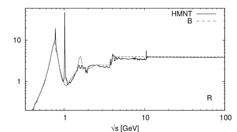
To arrive at a numerical result we adopt the following parametrizations for : For the comparison with earlier work [9] we take the function provided by H.Burkhardt [10]. This parametrization (denoted by B) is simple and efficient for the integration, however, it includes only data more than 20 years old. A newer parametrization (denoted by HMNT) is based on the most recent and accurate data and will be used for most of our detailed predictions. The two parametrizations for are shown in Fig. 7.
The contributions from narrow resonances are incorporated using:
| (52) |
For the parametrization HMNT we take , , , and as narrow resonances with the parameters listed in Table 1, thus replacing their rapidly varying cross section governed by a narrow Breit-Wigner shape with an easy to be integrated delta function.
| (GeV) | 3.096916(11) | 3.686093(34) | 9.46030(26) | 10.02326(31) | 10.3552(5) |
|---|---|---|---|---|---|
| (keV) | 5.55(14) | 2.48(6) | 1.340(18) | 0.612(11) | 0.443(8) |
| 0.957785 | 0.95554 | 0.932069 | 0.93099 | 0.930811 |
Parametrization B uses slightly different values and includes in addition , , , , , , , and as narrow resonances and we adopt the parameter values listed in the code [10]. For later use we also give the results for the moments , , and based on parametrization B:
| (53) |
|
|
|
|
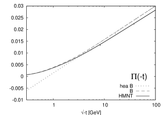
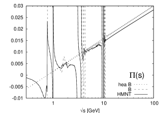
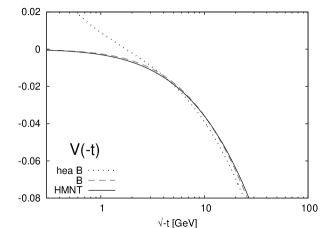
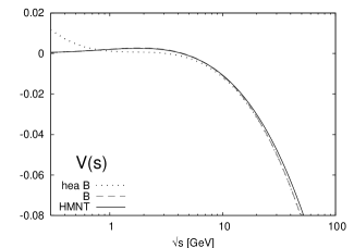
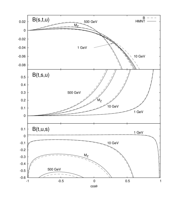
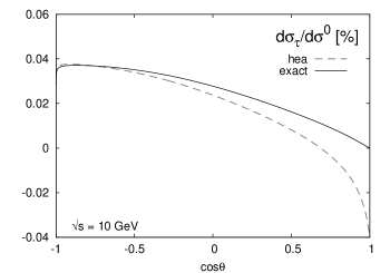
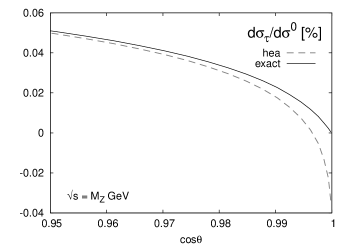
The results for the vacuum polarization and the vertex correction for space-like and time-like are shown in Fig. 8 as functions of . We display the predictions based on both parametrization B (dashed) and HMNT (solid). For comparison we also show the behaviour in the high energy approximation (dotted) of eq.(40-41), for parametrization B only. As expected from the comparison in Fig. 7, the difference between the two parametrization leads to differences in and of less than 10% which are unimportant for the two-loop analysis (the present uncertainty for HMNT amounts to typically one to two percent). For and the high energy approximation starts to deviate significantly from the full result for energies below 3 GeV, while for the resonant behaviour cannot be reproduced by this approximation. The corresponding results for the functions , which govern the behaviour of the irreducible box contribution are shown in Fig. 9 for a set of representative energies as functions of the scattering angle . The result for is obtained from through the substitution .
As expected, the predictions for , and based on the two paratrizations B and HMNT are always quite close, hence the following discussion will be based on HMNT only.
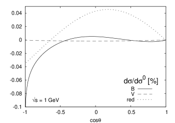
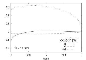
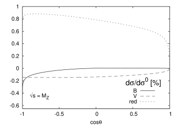
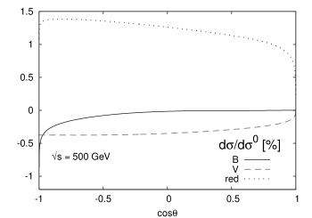
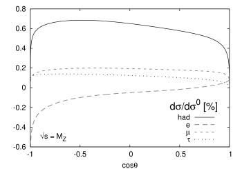
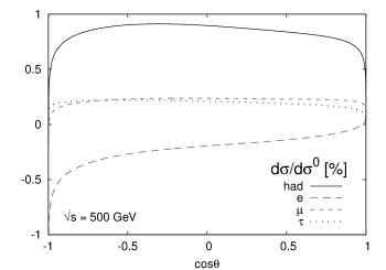
The corrections for the differential distributions are shown in Fig. 10 for four characteristic energies, normalized relative to the Born prediction333We do not present the two-loop vacuum polarization insertions of Eq.(8) which are best combined with the one-loop and Born contribution in the resummed form of Eq.(6). It is clear that must be known with a relative precision of about one percent, if one aims at luminosity determination with an error significantly below one per mille.. They are separated into those from reducible diagrams (), irreducible vertex () and box () diagrams444Here and below the infrared-sensitive contributions proportional to are set to zero.. In most of the cases the reducible ones are significantly larger than the irreducible ones, a consequence of their enhancement by the large logarithm .
|
|
|
|
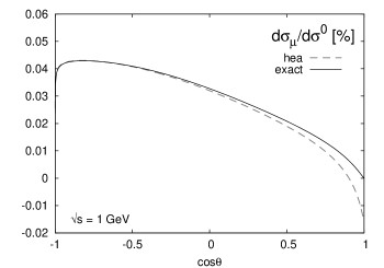
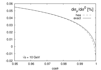
In Fig. 11 we display the corresponding contributions from muons (solid line) and leptons (dashed line), which can be evaluated similar to the hadronic ones. It is interesting to observe that the high energy approximation (hea) for the muon case, , (dotted) fails quite badly for small angles at GeV, a fact that could be anticipated already from Fig. 8, which shows the pour quality of this approximation for GeV in the hadronic case. For high energies, the quality of the approximation should be sufficient for all practical purposes (Fig. 11).
|
|
|
|
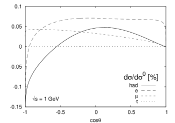
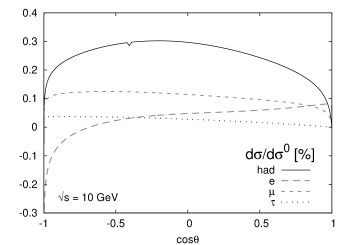
The relative corrections from hadron and lepton (, , ) loops are compared in Fig. 12. A markedly different energy and angular dependence is observed for the four contributions. Individually and in the sum, they significantly exceed the level of one per mille necessary to achieve the corresponding precision of the luminosity measurements. However, as discussed before, the reducible terms dominate and the irreducible hadronic terms are typically below one per mille. For precise comparisons the numerical results are also listed in Table 2 for a selected set of energies and angles. For small angles the box contribution remains tiny, often around or below of the Born cross section, and the result is dominated by the reducible correction which is typically a factor to larger and is trivially obtained from existing one-loop results, Eq.(13)-(3.2).
To illustrate the relative importance of reducible and irreducible contributions, the results for the irreducible box and the sum are listed in Table 3. The relative contribution of is evidently tiny. The results for are also compared with those from [9]. For the hadronic case they are in good agreement, although sometimes deviating in the last of the digits listed in [9]. For the leptons perfect agreement is observed.
|
|
|
|
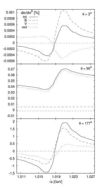
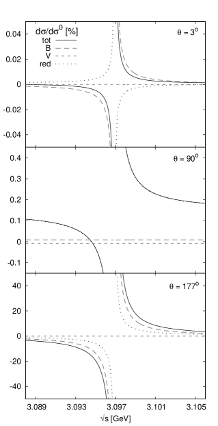
In general, the corrections exhibit a fairly smooth energy dependence. However, the situation changes for energies close to narrow resonances. This is exemplified in Fig. 13 for two cases: around the and around the resonances for three fixed angles: , and . The interference of the continuum amplitude with a Breit-Wigner enhanced correction is clearly visible. At (), irreducible box and the reducible corrections are of comparable size and opposite (equal) sign, at the reducible ones dominate. The vertex corrections are always small. Formally for the case of the , treated as narrow resonance, the correction even diverges, and it is still extremely large if the natural width of is introduced. In practice, however, the cross section has to folded with the energy spread of order MeV. In this case the singular amplitude with its asymmetric behaviour around is damped and thus remains a small correction. From these considerations, it is clear that a precise parametrization of is required in regions of rapidly varying cross section, if one aims at a precise prediction of the corrections in this region.
| GeV | GeV | |||||
| GeV | ||||||
| GeV | GeV | GeV | |||
| had | |||||
| GeV | GeV | GeV | |||
| had | |||||
The implementation of these results in a Monte Carlo generator is straightforward and their modular structure should lead to an efficient program. The reducible contribution can be obtained from the one-loop corrections simply modifying the photon propagators outside the loop according to:
| (54) |
and adding the terms proportional to multiplied by the imaginary part of the one-loop result. The irreducible vertex corrections can be directly combined with the Born cross section. All these are one-dimensional functions that can be tabulated once for ever. The irreducible box contribution is decomposedinto terms proportional to and plus a remainder characterized by the functions , , and . These are obtained through efficient and precise integration routines555available upon request from the authors..
|
|
6 Conclusions
Using published one-loop results, a compact formula has been derived which, in combination with dispersion relations and the by now well-measured R-ratio, can be used to evaluate the hadronic contributions to Bhabha scattering. The same approach is applicable for leptonic contributions, in particular from muons and -leptons. The method and result are valid in the limit for arbitrary and arbitrary . Comparing with [9], our numerical results are in perfect agreement for massive leptons, with arbitrary, while for hadronic contributions we observe small numerical differences. In the high energy limit the integrals can be evaluated in analytic form and the results have been compared with those for lepton loops that can be found in the literature. We find that overall size of the corrections, their sign and their angular dependence differ significantly between hadron, muon, -lepton and electron contributions. The size of the hadronic corrections varies from a fractional up to several permille. However, these are dominated by the reducible ones, with the irreducible box and vertex terms being typically below one permille. The modular structure of the results allows for a simple implementation into any Monte Carlo generator. For such an implementation, the corrections from virtual plus soft real photon radiation must be complemented by hard real radiation. This part is evidently straightforward, since it involves tree-level diagrams only, with the photon propagator dressed by hadronic vacuum polarization.
Acknowledgments
We would like to thank H. Burkhardt and T. Teubner for providing us with the parametrizations for the function and A. Penin and T. Teubner for helpful comments. Work supplied by BMBF contract 05HT4VKAI3.
References
- [1] A. A. Penin, Phys. Rev. Lett. 95 (2005) 010408 [arXiv:hep-ph/0501120], Nucl. Phys. B 734 (2006) 185 [arXiv:hep-ph/0508127].
- [2] Z. Bern, L. J. Dixon and A. Ghinculov, Phys. Rev. D 63 (2001) 053007 [arXiv:hep-ph/0010075].
- [3] T. Becher and K. Melnikov, JHEP 0706 (2007) 084 [arXiv:0704.3582 [hep-ph]].
-
[4]
M. Czakon, J. Gluza and T. Riemann,
Nucl. Phys. B 751 (2006) 1
[arXiv:hep-ph/0604101];
S. Actis, M. Czakon, J. Gluza and T. Riemann, Nucl. Phys. B 786 (2007) 26 [arXiv:0704.2400 [hep-ph]]. - [5] R. Bonciani, A. Ferroglia and A. A. Penin, JHEP 0802 (2008) 080 [arXiv:0802.2215 [hep-ph]], Phys. Rev. Lett. 100 (2008) 131601 [arXiv:0710.4775 [hep-ph]].
-
[6]
R. Bonciani, P. Mastrolia and E. Remiddi,
Nucl. Phys. B 661 (2003) 289
[Erratum-ibid. B 702 (2004) 359]
[arXiv:hep-ph/0301170],
Nucl. Phys. B 676 (2004) 399
[arXiv:hep-ph/0307295].
Nucl. Phys. B 690 (2004) 138
[arXiv:hep-ph/0311145];
R. Bonciani, A. Ferroglia, P. Mastrolia, E. Remiddi and J. J. van der Bij, Nucl. Phys. B 681 (2004) 261 [Erratum-ibid. B 702 (2004) 364] [arXiv:hep-ph/0310333]; Nucl. Phys. B 701 (2004) 121 [arXiv:hep-ph/0405275]. Nucl. Phys. B 716 (2005) 280 [arXiv:hep-ph/0411321]. -
[7]
M. Czakon, J. Gluza and T. Riemann,
Phys. Rev. D 71 (2005) 073009
[arXiv:hep-ph/0412164];
R. Bonciani and A. Ferroglia, Phys. Rev. D 72 (2005) 056004 [arXiv:hep-ph/0507047]. - [8] N. Cabibbo and R. Gatto, Phys. Rev. 124 (1961) 1577.
- [9] S. Actis, M. Czakon, J. Gluza and T. Riemann, Phys. Rev. Lett. 100 (2008) 131602 [arXiv:0711.3847 [hep-ph]]; S. Actis, J. Gluza and T. Riemann, arXiv:0807.0174 [hep-ph].
- [10] H. Burkhardt, TASSO-NOTE-192 and privat comunications.
-
[11]
Private communications, routine based on the data compilation of:
K. Hagiwara, A. D. Martin, D. Nomura and T. Teubner, Phys. Lett. B 649 (2007) 173 [arXiv:hep-ph/0611102], Phys. Rev. D 69 (2004) 093003 [arXiv:hep-ph/0312250]. - [12] B. A. Kniehl, M. Krawczyk, J. H. Kühn and R. G. Stuart, Phys. Lett. B 209 (1988) 337.
-
[13]
R. W. Brown, R. Decker and E. A. Paschos,
Phys. Rev. Lett. 52 (1984) 1192;
M. Bohm, A. Denner, T. Sack, W. Beenakker, F. A. Berends and H. Kuijf, Nucl. Phys. B 304 (1988) 463. - [14] G. J. H. Burgers, Phys. Lett. B 164 (1985) 167.
-
[15]
A. O. G. Källen and A. Sabry,
Kong. Dan. Vid. Sel. Mat. Fys. Med. 29N17 (1955) 1;
K. G. Chetyrkin, J. H. Kühn and M. Steinhauser, Nucl. Phys. B 482 (1996) 213 [arXiv:hep-ph/9606230] and references therein