HOW MUCH CAN WE LEARN FROM SN1987A EVENTS?
Or: An Analysis with a Two-Component Model for the Antineutrino Signal

Abstract

We analyze the data of Kamiokande-II, IMB, Baksan using a parameterized description of the antineutrino emission, that includes an initial phase of intense luminosity. The luminosity curve, the average energy of $\bar{\nu}_{e}$ and the astrophysical parameters of the model, derived by fitting the observed events (energies, times and angles) are in reasonable agreement with the generic expectations of the delayed scenario for the explosion.

INFN, Laboratori Nazionali del Gran Sasso, Assergi (AQ), Italy
E-mail: vissani@lngs.infn.it

and

INFN, Laboratori Nazionali del Gran Sasso, Assergi (AQ), Italy
L’Aquila University, Coppito (AQ), Italy
E-mail: giulia.pagliaroli@lngs.infn.it

1 Introduction

We begin with a rapid historical excursus, with emphasis on the issues that are relevant for data analysis.

• Colgate & White 1966^?) propose the paradigm for the explanation of the core collapse supernovae, where neutrinos are the key agents.

• Nadyozhin 1978^?) concludes a detailed calculation that demonstrates an initial phase of intense neutrino luminosity.

• Bethe & Wilson 1985^?) suggest that the energy deposition on a scale of half a second can re-energize the stalled shock wave.

• 1987: Kamiokande-II^?), IMB^?), Baksan^?) and LSD^?) observe several events in correlation with SN1987A.

• Several authors–e.g., Bahcall 1989^?)–remark that non-LSD data generically meet the expectations. Then the main interest shifts on the relevance of oscillations.

• Lamb & Loredo 2002^?) (LL) discuss whether SN1987A data indicate specific imprints of the delayed scenario such as the initial phase of intense luminosity.

• Imshennik & Ryazhskaya 2004^?) suggest a 2 stage scenario with essential role of rotation and possible explanation of LSD events detected 4.5 hours earlier.

Next we summarize the present status: although there is mounting evidence that the delayed scenario is correct, a conclusive proof is still missing; while most people is convinced that SN1987A neutrinos confirmed the general picture of the explosion, there are annoying doubts on whether SN1987A was a standard object or not; while we continue sharpening our theoretical tools, we hope intensely in a Galactic supernova event to progress in our understanding.

In short, one should be aware that until the theoretical picture will be definitively assessed, the interpretation of the results from SN1987A will continue to contain elements of uncertainty. But if we want to test the expectations, we are forced to answer the question: What are the generic expectations for the delayed scenario? We summarize the features that are relevant for our analysis:

• In conventional detectors (scintillators and water Cherenkov) the main detection reaction is the inverse-beta decay of electron antineutrinos on free protons (IBD): $\bar{\nu}_{e}p\to ne^{+}$.

  

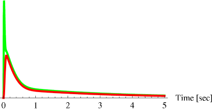
  Figure 1: Sketch of $\nu_{e}$ and $\bar{\nu}_{e}$ (higher and lower) luminosity curves. The excess of $\nu_{e}$ in the first 50 ms (‘neutronization’ phase) gives a small contribution to the total number of observable events.

• The main part of the emission happens in two stages as shown in Fig. 1. 10-20% of the energy is radiated in an early phase, here called accretion, that should last about half-a-second; 80-90% of the energy is radiated later, during the phase of neutron star cooling, namely in a quiet thermal phase.

• The main reactions for energy radiation during accretion are $e^{-}p\to n\nu_{e}$ and $e^{+}n\to p\bar{\nu}_{e}$, the second being the inverse of IBD. The presence around the nascent neutron star of an abundant amount of $e^{+}e^{-}$ plasma ensures a large flux of $\nu_{e}$ and $\bar{\nu}_{e}$, that are key ingredients to revive the stalled shock wave. [See Janka^?) for a review.]

• During the cooling phase, neutrinos of all species ($\nu_{e},\nu_{\mu},\nu_{\tau},\bar{\nu}_{e},\bar{\nu}_{\mu},\bar{\nu}_{\tau}$) are radiated with similar luminosities; this feature is occasionally called ‘equipartition’.

In this talk, based on a work in collaboration with M.L. Costantini and A. Ianni^?), we present an analysis of SN1987A data along these lines. We will compare two models for neutrino emission, namely the conventional one, when the neutrino emission is described by a ‘one-component’ (cooling) model, and a ‘two-component’ (cooling+accretion) model which resembles more closely the expectations of the delayed scenario. Preliminary results have been documented in^?,?,?,?); see also^?), in particular Sect. 3.2 there.

2 Analysis of SN1987A Observation with One-Component Model

2.1 The Conventional Model for $\bar{\nu}_{e}$ Emission (=Exponential Cooling)

This is the model adopted in most of the quantitative analyses of SN1987A events (the notable exception, to be discussed later, being the work of LL^?)). The thermal emission of the neutron star is parameterized by a black body model with a steadily decreasing temperature:

$$\left\{\begin{array}[]{l}\displaystyle\frac{dN_{c}}{dt\;dE}=\frac{R_{c}^{2}}{2\pi}\cdot\frac{E^{2}}{1+\exp[E/T_{c}(t)]}\\[8.61108pt] \mbox{with }T_{c}(t)=T_{c}\cdot\exp[-t/(4\tau_{c})]\end{array}\right.$$ (1)

where the suffix $c$ means ‘cooling’ and where we use for convenience the natural units $\hbar=c=k_{B}=1$. The 3 parameters of the model are:

1. the neutrinosphere radius $R_{c}$ that describes the intensity of the emission;

2. the initial temperature $T_{c}$ that fixes the average energy of $\bar{\nu}_{e}$;

3. the luminosity time scale $\tau_{c}$ that quantifies the duration of the process.

An isotropic emission from $D=50$ kpc is assumed so that the flux is simply $\Phi_{c}=1/(4\pi D^{2})\times dN_{c}/dEdt$. For obvious reasons, this model for the antineutrino emission is called ‘exponential cooling’.

2.2 Procedure of Analysis

Next we describe the procedure of analysis we adopted. It is significantly more complex than the usually followed procedures (though we verified a posteriori none of these technical improvements leads to qualitative changes in the conclusion) and elaborates on the results obtained by LL^?):
a) Since the absolute times of Kamiokande-II and Baksan are not measured precisely, and the time between the first neutrino and the first event in IMB is unknown, we use only the relative times of the events ($t_{1}=0$ for any detector).
b) Since the duration of the signal is not known a priori, we consider the data in a unified time window of 30 s.
c) We account for the measured background (Kamiokande-II and Baksan), dead-times and angular-bias (IMB).
d) We account for the error in the energy measurement in all detectors. More details of the analysis are described in Appendices A and B.
The expected number of signal events obtained from the differential rate

$$\frac{dN}{dtdE_{e}d\cos\theta}=N_{p}\frac{d\sigma_{\bar{\nu}_{e}p}}{d\cos\theta}(E_{\nu},\cos\theta)\Phi_{\bar{\nu}_{e}}(t,E_{\nu})\xi_{d}(\cos\theta)\eta_{d}(E_{e})\frac{dE_{\nu}}{dE_{e}},$$ (2)

that requires to know the number of protons in the detector, the interaction (IBD) cross section, the $\bar{\nu}_{e}$ flux, the angular bias, the detection efficiency and the Jacobian.

2.3 Results

A straightforward fit yields the following values of the three astrophysical parameters

$$R_{c}=26\mbox{ km},\ T_{c}=4.5\mbox{ MeV},\ \tau_{c}=3.9\mbox{ s}\$$ (3)

while the best fit of the offset times are zero, due to the fact that the signal is bounded to decrease with time. Our best fit is very close to the value in Bahcall book.^?)

The difference with LL is mostly due to their treatment of efficiency–not of background, inclusion of angles, or better cross section. Indeed, LL include efficiency in the exponential of $e^{\!-\!\sum\mu_{j}(\rm with)}\prod\mu_{i}(\rm w/o)$, we include it in both terms. A formal justification of our procedure is given in Appendix A.

2.4 Should We Stop Here?

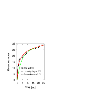
Figure 2: Temporal distribution of the events; the end of the first second is marked by a dashed line.

At this point we face the question: should we be content of the generic agreement with the expectation and stop the analysis here? One could presume that Bahcall would have answered “yes”. Indeed, in his book,^?) the analysis of SN1987A data is introduced by the statement:

Unfortunately, a “minimum” model has proven adequate to describe the sparse amount of data.

The study of the ‘exponential cooling’ model is then commented with the sentence:

The success of this simplified “standard” model suggests that it will be difficult to use the neutrino events observed from SN1987A to establish more detailed models.

We wish to note that “difficult” does not mean “impossible” and, remaining aware of this authoritative opinion, we would like to continue the discussion begun by Lamb & Loredo: whether it is worthwhile to go beyond the exponential cooling model.

Actually, observations offer us some motivation to proceed. In fact, there is a hint of an increased luminosity in the first second. This is evident from Fig. 2, where we show the temporal distribution of the observed events, from^?) (see also^?)). For comparison, we show also two time distributions, comprising also 7 background events (the expectations is 5.6 in Kamiokande-II and 1 in Baksan). In the lower one, all 22 signal events belong to the cooling component. In the upper one, only 13 signal events belong to cooling; the remaining 9 belong to the accretion component. In the figure it is indicated the GOF of these two hypotheses, evaluated with a Smirnov-Cramèr-Von Mises test.

3 Analysis of SN1987A Observation with Two-Component Model

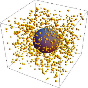
$$\ \ \ \ \ \ \ \ \ \ \ \ \ \ \ \ \ \ \ \ \ \ \ \ \ \ \ \ \ \ \ \ \ \ \ \ \ \ \ \ \begin{array}[]{l}\mbox{\tt Thermal $e^{+}$'s react}\\[-3.44444pt] \mbox{\tt on target neutrons}\\[0.0pt] \ \ \ \displaystyle N_{n}(t)=\frac{Y_{n}\ M_{a}(t)}{m_{n}}\\[-0.86108pt] \mbox{\tt yielding many $\bar{\nu}_{e}$'s.}\end{array}$$

Figure 3: The yellow (gray) centers surrounding the NS (dark gray) represent pictorially the individual reactions $e^{-}p\to n\nu_{e}$ and $e^{+}n\to p\bar{\nu}_{e}$ occurring during accretion.

3.1 How to Describe the Initial Emission (=Accretion)

The initial emission is dominated by the quasi-transparent accreting region: on top of the previous black body emission, we simply need to model the radiation of $\bar{\nu}_{e}$ from $e^{+}n\to p\bar{\nu}_{e}$. Quite directly, we use:

$$\frac{dN_{a}}{dtdE}=\frac{1}{\pi^{2}}N_{n}(t)\sigma_{e^{+}n}(E_{\nu})\frac{E_{e}^{2}}{1+\exp[E_{e}/T_{a}(t)]}$$ (4)

The conceptual scheme is represented pictorially in Fig. 3, where the second astrophysical parameter $M_{a}$ (the accreting mass) besides the temperature of the positron plasma, is introduced. The assumed description of how $T_{a}$ and $M_{a}$ evolve in time is given in Appendix B, but it should be not a surprise that this description brings in a third parameter, $\tau_{a}$, the duration of the process of accretion. We compare in the next page our description of $\bar{\nu}_{e}$ emission with the one suggested by Lamb and Loredo.

The energy spectrum of our model, for selected values of the astrophysical parameters, is given in Fig. 4 (from^?)). The spectrum is ‘pinched’ and for the selected values of the astrophysical parameters it has a ‘pinching’ factor of about $\sim 4$ (note that the ‘pinching’ is an output, not an input).

Figure 4: Continuous curve: $\bar{\nu}_{e}$ flux for $M_{a}=0.15\ M_{\odot}$ and $T_{a}=2.5$ MeV. Dotted curve: black body distribution with the same luminosity ($1.1\times 10^{53}$ erg/s) and average energy ($13$ MeV), namely, with parameters $R_{c}=82$ km and $T_{c}=4.1$ MeV.

3.2 Results

Following the same procedure adopted for the one-component model, we obtain the values of the astrophysical parameters:

Lamb & Loredo Model

The best fit point is^?):

$$\begin{array}[]{ccc}R_{c}=12\mbox{ km},&T_{c}=5.5\mbox{ MeV},&\tau_{c}=4.3\mbox{ s},\\ M_{a}={5.5\ M_{\odot}},&T_{a}={1.5\mbox{ MeV}},&\tau_{a}={0.7\mbox{ s}}.\end{array}$$ (5)

The big value of $M_{a}$ and the small value of $T_{a}$ are dictated by KII early events. The luminosities and average energies are given in Fig. 5. The sharp transition at $t\sim\tau_{a}$ does not look very appealing, when compared with the result of a typical simulation.^?)

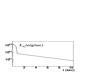
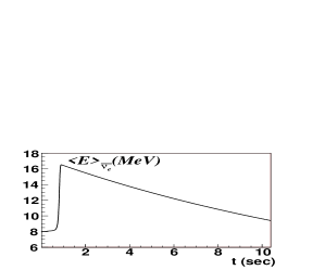
Figure 5: LL model: antineutrino luminosity and average energy in the best fit point.

Pagliaroli et al. Model

The best fit point is^?):

$$\begin{array}[]{ccc}R_{c}=16\mbox{ km},&T_{c}=4.6\mbox{ MeV},&\tau_{c}=4.7\mbox{ s},\\ M_{a}={0.2\ M_{\odot}},&T_{a}={2.4\mbox{ MeV}},&\tau_{a}={0.6\mbox{ s}}.\end{array}$$ (6)

Note that $M_{a}$ is much smaller and at the same time $T_{a}$ increased. The luminosity and average energy curves of Fig. 6 are much more regular and in much better agreement with the expectations.^?)

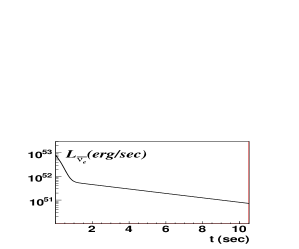
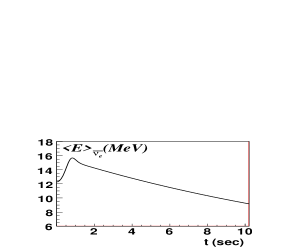
Figure 6: Pagliaroli et al. model: antineutrino luminosity and average energy in the best fit point.

One may ask: what are the main reasons of the different result? This is answered by Tab. 1 from^?), where we show the effect of the various modification on the best fit point and we indicate the improvement of the two-component models in comparison with the exponential cooling model. The two main differences of our model for antineutrino emission with the model due to LL are 1) that we assume a time dependent temperature $T_{a}$, that makes the average antineutrino energy continuous; 2) that, differently from LL, we postpone the occurrence of the cooling phase to the end of the accretion phase. In such a manner we have an approximately thermal spectrum at any time, as expected,^?) and we remove the bi-modality that characterizes the first second of emission in the LL model. It should be noted that these defects of the LL model have been noted already in Mirizzi and Raffelt^?).

Subsequent	$R_{c}$	$T_{c}$	$\tau_{c}$	$M_{a}$	$T_{a}$	$\tau_{a}$	Signif.
improvement	[km]	[MeV]	[s]	[$M_{\odot}$]	[MeV]	[s]	[%]
technical ($\approx$LL)	12	5.5	4.3	5.6	1.5	0.7	99.8
$T_{a}(t)$	14	5.0	4.8	0.8	1.8	0.7	98.9
time shift	14	4.9	4.7	0.1	2.4	0.6	98.0
oscillations	16	4.6	4.7	0.2	2.4	0.6	98.0

Table 1: Best-fit values of astrophysical parameters. Each line of this table is an incremental step toward the final improved parameterization. Last column shows the significance of the 2-component models in comparison (likelihood-ratio test, +3 d.o.f.) with the exponential cooling model.

The two-component models are better than the exponential cooling model. As a matter of fact, the LL-model would seem to fare better in describing the data, but it deviates more strongly from the expectations of the delayed scenario than our model. Indeed, the LL model has less difficulty to account for the large difference between the energies detected by Kamiokande-II and IMB in the first second, since it can ascribe these two datasets to two different but contemporaneous phases of emission. This bi-modality is forbidden by construction in our model.

3.3 Errors in the Pagliaroli et al. Model

The error on the astrophysical parameters can be determined from the data^?):

$$\begin{array}[]{ll}R_{c}=16^{+9}_{-5}\rm\ km,&M_{a}=0.22^{+0.68}_{-0.15}\ M_{\odot},\\ T_{c}=4.6^{+0.7}_{-0.6}\rm\ MeV,&T_{a}=2.4^{+0.6}_{-0.4}\rm\ MeV,\\ \tau_{c}=4.7^{+1.7}_{-1.2}\rm\ s,&\tau_{a}=0.55^{+0.58}_{-0.17}\rm\ s.\end{array}$$ (7)

We also show the values of the offset times:

$$t^{\mbox{\tiny off}}_{{\mbox{\tiny KII}}}=0.^{+0.07}\rm\ s,\ t^{\mbox{\tiny off}}_{\mbox{\tiny IMB}}=0.^{+0.76}\rm\ s,\ t^{\mbox{\tiny off}}_{{\mbox{\tiny BAK}}}=0.^{+0.23}\rm\ s.$$ (8)

We see that the limited statistics manifests itself in relatively large errors.

The marginal distributions for accretion parameters $M_{a}$ and $T_{a}$ of $\bar{\nu}_{e}$ and for cooling parameters $R_{c}$ and $T_{c}$ of $\bar{\nu}_{e}$ with the complete emission model are given in Ref.^?). Other solutions exist^?) at $M_{a}\sim M_{\odot}$. Here we discarded them, considering that in the delayed scenario, $M_{a}$ should be a fraction of the outer core mass $M_{oc}\approx 0.6\ M_{\odot}$.

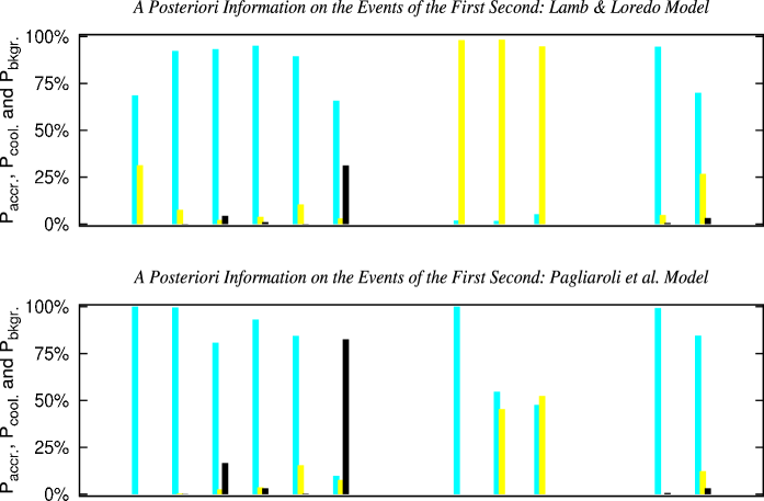
Figure 7: Events in the first second: 6 in KII, 3 in IMB, 2 in Baksan. First bar (light blue/gray), accretion probability; second bar (yellow/light gray), cooling probability; third bar (black), background probability.

3.4 Meaning of the Individual Events

Given a theoretical model for antineutrino emission, we can evaluate the meaning of each individual event. This is given in^?) in table form and also in Fig. 7 in graphical form for the 11 events detected in the first second and using the best fit models. We derive two principal conclusions:
$i)$ First, all 11 events are mostly due to signal and not to background, with the exception of the event number six of Kamiokande-II that is below the energy threshold of 7.5 MeV. The background probability of this event is larger in the model by Pagliaroli et al., due to the fact that it happened 0.686 s after the first one, namely, in the moment when the average energy of antineutrinos is maximal: see Fig. 6.
$ii)$ Second, we see from Fig. 7 that in the LL model, the 3 events of IMB are attributed to cooling, the 6 events of Kamiokande-II to accretion. This is a manifestation of the bi-modality of the LL model noted previously: the cooling and the accretion phases are assumed to be contemporaneous and with very different average energies. Thus the (low energy) events of Kamiokande-II are easily explained by accretion, the (high energy) ones of IMB by cooling. In the other model^?) the spectrum is not bi-modal by construction. Thus the 11 events are treated on equal footing and all of them (including IMB’s) have a high probability to be due to accretion.

Another manifestation of the bi-modality of the LL model is the great difference between the time integrated spectra of accretion and of cooling; see Fig. 2 of Ref.^?). This implies that the resulting total spectrum cannot described by a thermal distribution, even including a ‘pinching’ factor.

4 Conclusions

Our study confirms earlier results with the 1-component model. The refined treatment of background, cross section, description of the scattering angle, inclusion of Baksan data, etc. do not lead to important changes.

We confirm the results of Lamb & Loredo in particular the very strong evidence for accretion, when their 2-component model is adopted.

We discussed an improved 2-component model, where the average energy and luminosity curves are constrained to be continuous, cooling follows accretion, oscillations (not very important a posteriori) are included.

The best fit of $\tau_{a}$, $M_{a}$, etc. are close to expectations; the binding energy $2.2\times 10^{53}$ erg is lower than for the 1-component model; the evidence of accretion is not as strong as for the Lamb & Loredo model, but still important.

5 Acknowledgments

F.V. is very grateful to Milla Baldo-Ceolin for the very honorable invitation. We thank A. Ianni and M.L. Costantini for the stimulating collaboration, upon which this work is based.

Appendix A: Derivation of the Likelihood Function

We present here a derivation of the likelihood function that follows the one given in Appendix A of LL, but notations and conclusions are somewhat different. For a given model of the detector and of the antineutrino signal, we construct the likelihood:

$${\cal L}=\prod_{i=1}^{N}P_{i}\mbox{ where }P_{i}=\left\{\begin{array}[]{l}P(d=0)\mbox{ if no events are detected in the $i$-th bin}\\ P(d(x_{i}))\mbox{ if one event is detected in the $i$-th bin}\end{array}\right.$$ (A.1)

the $i$=th time-bin being located in

$$(i-1)\delta t\leq t<i\delta t$$ (A.2)

Of course, $d=0$ means that no event was detected in the given time bin. $d(x)$ means that one event was detected in the time-bin with coordinates (namely: energy, direction and position) generically denoted as $x$. The product is on the number of time bins, $N$, each one of size $\delta t$; $T=N\delta t$. The number of bins is much larger than the number of detected events, $N\gg N_{d}$. The two types of probability are calculated as follows:

$$\begin{array}[]{lcl}P(d=0)&\simeq&P(d=0,e^{+}=0,b=0)+\\ &&P(d=0,e^{+}=0,b=1)+\\ &&P(d=0,e^{+}=1,b=0)\\[4.30554pt] P(d(x))&\simeq&P(d(x),e^{+}=0,b=1)+\\ &&P(d(x),e^{+}=1,b=0)\end{array}$$ (A.3)

namely by considering the various cases, when the given time bin contains 0 or 1 events due to background, $b$, or due to positrons produced in the detector, $e^{+}$. This separation might appear cumbersome at first sight but it helps for comparing with Appendix A of LL. The notation $e^{+}=1$ ($b=1$) means that one positron (one background event) was in the detector in the given time bin, with some value of the the coordinates; similarly, $d=1$ means that one event was detected in the given time bin, with some value of the the coordinates.

Now we will expand the five terms in Eq. A.3 to order ${\cal O}(\delta t)$.

We begin with the simplest case when no event is present:

$$\begin{array}[]{l}P(d=0,e^{+}=0,b=0)=\\ P(d=0,e^{+}=0|b=0)\times P(b=0)=\\ P(d=0|e^{+}=0,b=0)\times P(e^{+}=0)\times P(b=0)=\\ 1\times\exp(-S_{+}(t)\delta t)\times\exp(-B\delta t)=\\ 1-\delta t(S_{+}(t)+B)\end{array}$$ (A.4)

where we introduced the positron production rate $S_{+}(t)$, the (time independent) background rate $B$ and assumed Poisson statistics for both processes.

The next two cases have one background event but no positron produced:

$$\begin{array}[]{l}P(d=0,e^{+}=0,b=1)\equiv 0\\[4.30554pt] P(d(x),e^{+}=0,b=1)\equiv\delta tB(x)\end{array}$$ (A.5)

This is basically a definition of what we mean by background: The background is a detected event that is not due to the signal. Note that we are not attempting to describe the nature of the background with this procedure, we are simply taking into account its existence. However, having assumed that the average background is independent from the time of observation, there is practical way to obtain $B(x)$; this can be measured by the experimental collaborations in the instants of time when the signal is absent.

The more complicate cases are the remaining two, when a positron is produced. Adopting the symbol $x_{+}$ for the coordinates of the positron, we get:

$$\begin{array}[]{l}P(d=0,e^{+}=1,b=0)=\\ \int dx_{+}P(d=0,e^{+}(x_{+}),b=0)=\\ \int dx_{+}P(d=0,e^{+}(x_{+})|b=0)\times P(b=0)=\\ \int dx_{+}P(d=0|e^{+}(x_{+}),b=0)\times P(e^{+}(x_{+}))\times P(b=0)=\\ \int dx_{+}(1-\eta(x_{+}))\times S_{+}(t,x_{+})\delta t\times 1=\\ \delta t(S_{+}(t)-\int dx_{+}\eta(x_{+})S_{+}(t,x_{+}))=\\ \delta t(S_{+}(t)-S(t))\end{array}$$ (A.6)

where we used $P(e^{+}(x_{+}))=S_{+}(t,x_{+})\delta t\ \exp(-S_{+}(t,x_{+})\delta t)$ and introduced the definition of detection efficiency, that agrees with the one of LL:

$$P(d=0|e^{+}(x_{+}),b=0)=1-\eta(x_{+})$$ (A.7)

The last term to evaluate is:

$$\begin{array}[]{l}P(d(x),e^{+}=1,b=0)=\\ \int dx_{+}P(d(x),e^{+}(x_{+}),b=0)=\\ \int dx_{+}P(d(x),e^{+}(x_{+})|b=0)\times P(b=0)=\\ \int dx_{+}P(d(x)|e^{+}(x_{+}),b=0)\times P(e^{+}(x_{+}))\times P(b=0)=\\ \int dx_{+}\rho(x,x_{+})\eta(x_{+})\times S_{+}(t,x_{+})\delta t\times 1=\\ \delta t\int dx_{+}\rho(x,x_{+})\eta(x_{+})S_{+}(t,x_{+}))=\\ \delta tS(t,x)\end{array}$$ (A.8)

where the last equality is simply the definition of $S(t,x)$.

We introduced the new function $\rho(x,y)$ according to:

$$P(d(x)|e^{+}(x_{+}),b=0)\equiv\rho(x,x_{+})\eta(x_{+})$$ (A.9)

The interpretation of this function is as follows. When we consider the probability that a positron is either detected or missed, we should get 1:

$$P(d=0|e^{+}(x_{+}),b=0)+P(d=1|e^{+}(x_{+}),b=0)=1$$ (A.10)

In formulae and with the definitions introduced above:

$$1-\eta(x_{+})+\int dx\rho(x,x_{+})\eta(x_{+})=1$$ (A.11)

that implies $\int dx\rho(x,x_{+})=1$. Thus, $\rho(x,x_{+})$ can be thought of as the probability that the event produced with coordinates $x_{+}$ and eventually detected, will be observed with coordinates $x$: $\rho(x,x_{+})\equiv P(d(x)|e^{+}(x_{+})\ ,\ e^{+}\mbox{ detected})$. This function is occasionally called ‘smearing’, since a positron with well-defined coordinates will be mapped by the detector response into a wide set of coordinates of the detected event. This concludes the calculation of the five terms in Eq. A.3.

Plugging the results of Eqs. A.4, A.5, A.6 and A.8 in Eq. A.3 we find that the expression of the probabilities in the given time bin at the order $\delta t$:

$$\begin{array}[]{ll}P(d=0)&=(1-\delta t(S_{+}(t)+B))+0+\delta t(S_{+}(t)-S(t))\simeq\\ &\simeq e^{-\delta t(B+S(t))}\\[4.30554pt] P(d(x))&=\delta t(B(x)+S(t,x))\simeq\\ &\simeq\delta t(B(x)+S(t,x))e^{-\delta t(B+S(t))}\end{array}$$ (A.12)

These can be introduced in the formula for the likelihood finding:

$${\cal L}=e^{-\int_{0}^{T}dt(B+S(t))}\prod_{i=1}^{N_{d}}\delta t(B(x_{i})+S(t_{i},x_{i}))$$ (A.13)

We can omit the multiplying, constant factors $\exp(-BT)$ and $(\delta t)^{N_{d}}$ without affecting the parameter estimations. We note finally that, owing to the definitions of $S(t)$ and $S(t,x)$, it is possible and occasionally convenient to define a detector-weighted interaction rate by including the efficiency $\eta(x_{+})$ in the positron production rate:

$$R(t,x_{+})\equiv S_{+}(t,x_{+})\eta(x_{+})$$ (A.14)

The likelihood becomes

$${\cal L}=\mbox{const.}\times e^{-\int_{0}^{T}dtdxR(t,x)}\prod_{i=1}^{N_{d}}(B(x_{i})+\int dx\rho(x_{i},x)R(t_{i},x))$$ (A.15)

Appendix B: Details of the Pagliaroli et al. Model

We estimate the theoretical parameters by the $\chi^{2}$:

$$\chi^{2}\equiv-2\sum_{d=k,i,b}\log({\cal L}_{d}),$$ (B.1)

where ${\cal L}_{d}$ is the likelihood of any detector ($k,i,b$ are shorthands for Kamiokande-II, IMB, Baksan). The likelihood of each of the 3 detectors is:

$$\begin{array}[]{l}{\cal L}_{d}=e^{-f_{d}\int\!\!R(t)dt}\times\prod^{N_{d}}_{i=1}e^{R(t_{i})\tau_{d}}\times\left[B(E_{i},\cos\theta_{i})+\int dE\rho(E,E_{i})R(t_{i},E,\cos\theta_{i})\right].\end{array}$$ (B.2)

Setting $f_{d}=1$ and $\tau_{d}=0$ (that is adequate for Kamiokande-II and Baksan) and noting that the IBD reaction is only weakly directional (that implies that the smearing on the angle can be in good approximation neglected) we see that this is equivalent to the likelihood discussed in detail just above.

The time dependent temperature is described as:

$$T_{a}(t)=T_{i}+(T_{f}-T_{i})\left(\frac{t}{\tau_{a}}\right)^{m}\!\!\mbox{ with }\left\{\begin{array}[]{l}T_{i}=T_{a}\\ T_{f}=0.6\ T_{c}\end{array}\right.$$ (B.3)

with $m=1-2$. The drop of the number of neutrons with time is:

$$N_{n}(t)=\frac{Y_{n}}{m_{n}}\times M_{a}\times\left(\frac{T_{a}}{T_{a}(t)}\right)^{6}\times\frac{j(t)}{1+t/0.5\mbox{ s}}$$ (B.4)

where $Y_{n}=0.6$ and

$$j(t)=\exp[-(t/\tau_{a})^{2}]$$ (B.5)

The time shift described as follows:

$$\Phi_{\bar{\nu}_{e}}(t)=\Phi_{a}(t)+(1-j(t))\times\Phi_{c}(t-\tau_{a})$$ (B.6)

Finally we give some details of the treatment of oscillations: For normal mass hierarchy (used in the calculation given in the main text) the survival probability and the observed $\bar{\nu}_{e}$ flux are:

$$\begin{array}[]{ll}P=U_{e1}^{2},\\[4.30554pt] \Phi_{\bar{\nu}_{e}}=P\ \Phi_{\bar{\nu}_{e}}^{0}+(1-P)\ \Phi_{\bar{\nu}_{\mu}}^{0},\\ \end{array}$$ (B.7)

For inverted mass hierarchy $\nu-\nu$ interaction introduces a swap between the $\bar{\nu}_{e}$ and $\bar{\nu}_{x}$ so that

$$\begin{array}[]{ll}P=U_{e1}^{2}P_{f}+U_{e3}^{2}(1-P_{f}),\\[4.30554pt] \Phi_{\bar{\nu}_{e}}=P\ \Phi_{\bar{\nu}_{\mu}}^{0}+(1-P)\ \Phi_{\bar{\nu}_{e}}^{0}.\\ \end{array}$$ (B.8)

The earth matter effect is described by the PREM model.

Appendix C: Discussion at the Workshop

We report the discussion at the Workshop after the talk was delivered. This discussion emphasizes certain important points and it is (at least in our view) useful, but since we were not able to reproduce the exact words used we apologize in advance (and take the full responsibility) for possible misunderstanding.

Q [P. Vogel]: Don’t angular distributions disagree with expectations? In particular, IMB’s? If you find the GOF is bad, you could doubt that such an analysis is legitimate.

A: The GOF of the angular distribution is discussed in our previous publication, PRD70:043006,2004. It is better than the conventional 5%, so the problem is not so severe as one may feel. Our re-evaluation of GOF and also the analysis uses the newly calculated cross section (PLB564:42-54,2003) and the published angular bias of IMB^?).
Again on IMB, there is an important point to note: the events of IMB cannot be elastic scattering events, because they are not so directional. And even being ready to consider something exotic taking place, it is hard to imagine a reaction that is forward peaked but too much, as needed to locate half of the events of IMB in the region where they are, $30^{\circ}<\theta<60^{\circ}$. All in all, the hypothesis that they are inverse beta decay events seems to be the most reasonable and conservative.
Other Authors explore the hypothesis that IMB analysis could be biased, e.g., Malgin in Nuovo Cim.C21:317-329,1998 (that incidentally also proposes interesting remarks on the time distribution of the events): this is not the case of our work on SN1987A events.

Q [V. Berezinsky]: The role of rotation is important and should be included in the analysis.

A: We tried to avoid linking our analysis to a specific model, and we kept the parameters free. These results could be used as follows: Suppose that a certain model with rotation produces an initial temperature of accretion $T_{a}$ much lower than the one of our best fit value; then, one could be entitled to conclude that this model with rotation is disfavored by the observations of SN1987A neutrino events.

Q [V. Matveev]: Could some events be due to neutrino interactions with iron?

A: Yes the most complete analysis should take into account all the interactions happening in the detectors. We tried to keep this analysis as simple as possible and this is the reason why we mainly focused on the parameterization of the most important flux, namely, the one of electron antineutrinos. As emphasized in the paper of Imshennik and Ryazhskaya^?), in order to assess the importance of the interactions with iron, we would need to describe the electron neutrino flux, too.

References

- [1] S. A. Colgate and R. H. White, “The Hydrodynamic Behavior of Supernovae Explosions,” Astrophys. J. 143 (1966) 626.
- [2] D. K. Nadyozhin, “The neutrino radiation for a hot neutron star formation and the envelope outburst problem,” Astrophys. Space Sci. 53 (1978) 131.
- [3] H. A. Bethe and J. R. Wilson, “Revival of a stalled supernova shock by neutrino heating,” Astrophys. J. 295 (1985) 14.
- [4] K. Hirata et al [Kamiokande-II Collaboration], “Observation of a Neutrino Burst from the Supernova SN1987A,” Phys. Rev. Lett. 58 (1987) 1490; K. S. Hirata et al. [Kamiokande-II Collaboration], “Observation in the Kamiokande-II Detector of the Neutrino Burst from Supernova SN 1987a,” Phys. Rev. D 38 (1988) 448; M. Koshiba, these Proceedings.
- [5] R. M. Bionta et al. [IMB Collaboration], “Observation of a Neutrino Burst in Coincidence with Supernova SN1987A in the Large Magellanic Cloud,” Phys. Rev. Lett. 58 (1987) 1494; C. B. Bratton et al. [IMB Collaboration], “Angular Distribution Of Events From SN1987A,” Phys. Rev. D 37 (1988) 3361.
- [6] E.N. Alekseev, L.N. Alekseeva, I.V. Krivosheina and V.I. Volchenko, “Detection of the neutrino signal from SN1987A in the LMC using the INR Baksan underground scintillation telescope,” Phys.Lett.B 205 (1988) 209.
- [7] M. Aglietta et al., “On the event observed in the Mont Blanc Underground Neutrino observatory during the occurrence of Supernova 1987a,” Europhys. Lett. 3 (1987) 1315.
- [8] J. N. Bahcall, chap. 15 of Neutrino astrophysics, Cambridge University Press, 1989.
- [9] T. J. Loredo and D. Q. Lamb, “Bayesian analysis of neutrinos observed from supernova SN 1987A,” Phys. Rev. D 65 (2002) 063002.
- [10] V. S. Imshennik and O. G. Ryazhskaya, “A rotating collapsar and possible interpretation of the LSD neutrino signal from SN 1987A,” Astron. Lett. 30 (2004) 14 [arXiv:astro-ph/0401613].
- [11] H.Th. Janka, “Conditions for Shock Revival by Neutrino Heating in Core-Collapse Supernovae,” A&A, 368 (2001) 527.
- [12] G. Pagliaroli, F. Vissani, M. L. Costantini and A. Ianni, “Improved Analysis of SN1987A Antineutrino Events,” preprint LNGS/TH-01/08.
- [13] F. Vissani, talk given at Symposium “20th anniversary of SN 1987A,” Moscow, Russia; with G. Pagliaroli, proceedings submitted to Astronomy Letters.
- [14] G. Pagliaroli, M. L. Costantini, A. Ianni and F. Vissani, “The first second of SN1987A neutrino emission,” arXiv:0705.4032 [astro-ph].
- [15] G. Pagliaroli, M. L. Costantini and F. Vissani, “Analysis of Neutrino Signals from SN1987A,” Proceedings of IFAE 2007, page 225, eds. G. Carlino, G. D’Ambrosio, L. Merola, P. Paolucci, G. Ricciardi, arXiv:0804.4598 [astro-ph].
- [16] F. Vissani, talk at XXVIII Encontro Nacional de Física de Partículas e Campos, Àguas de Lindóia, Brazil.
- [17] M. L. Costantini, A. Ianni, G. Pagliaroli and F. Vissani, JCAP 0705 (2007) 014 [arXiv:astro-ph/0608399].
- [18] See e.g., T. Totani, K. Sato, H.E. Dalhed, J.R. Wilson, “Future detection of a supernova neutrino burst and explosion mechanism,” Astrophys. J 496 (1998) 216 [arXiv:astro-ph/9710203] Fig.s 1,2 and 4; compare with A. Marek and H. T. Janka, “Delayed neutrino-driven supernova explosions aided by the standing accretion-shock instability,” arXiv:0708.3372 [astro-ph] Fig. 9.
- [19] The small deviations from a thermal spectrum have been discussed, e.g., in H.-T. Janka and W. Hillebrandt, Astron. & Astrophys. 224 (1989) 49 and more recently M.T. Keil, G.G. Raffelt and H.-T. Janka, “Monte Carlo study of supernova neutrino spectra formation,” Astrophys. J. 590 (2003) 971.
- [20] A. Mirizzi and G. G. Raffelt, “New analysis of the SN 1987A neutrinos with a flexible spectral shape,” Phys. Rev. D 72 (2005) 063001.