Extrasolar Giant Planets and X-ray Activity

Abstract

We have carried out a survey of X-ray emission from stars with giant planets, combining both archival and targeted surveys. Over 230 stars have been currently identified as possessing planets, and roughly a third of these have been detected in X-rays. We carry out detailed statistical analysis on a volume limited sample of main sequence star systems with detected planets, comparing subsamples of stars that have close-in planets with stars that have more distant planets. This analysis reveals strong evidence that stars with close-in giant planets are on average more X-ray active by a factor $\approx 4$ than those with planets that are more distant. This result persists for various sample selections. We find that even after accounting for observational sample bias, a significant residual difference still remains. This observational result is consistent with the hypothesis that giant planets in close proximity to the primary stars influences the stellar magnetic activity.

1 Introduction

After centuries of ignorance on planetary systems beyond our own, we are now in an era when stars are being routinely identified as possessing planets. Since the discovery by Mayor & Queloz (1995) of a Jupiter-type planet (mass $0.44~{}M_{J}$) orbiting close in to the G2 star 51 Peg ($0.05$ AU), almost three hundred new Extrasolar Giant Planets (EGPs) have been found.

One of the surprising results so far have been the detection of planets with orbital radii, ${a_{P}}$, much smaller than seen in the Solar System, with values as low as ${a_{P}}\approx$0.03 AU. At such small separations, it is likely that these giant planets will have measurable tidal ($\propto{a_{P}}^{-3}$) or magnetic ($\propto{a_{P}}^{-2}$ for large ${a_{P}}$) effects on the primary stars (Cuntz, Saar, & Musielak 2000; Saar, Cuntz, Shkolnik 2004). Both these effects increase non-linearly for small values of ${a_{P}}$, leading to potentially dramatic disruptions of the stellar environment for stars with close-in giant planets. How these disruptions affect coronal activity remains an open question. It is possible that activity will be enhanced because of the magnetic interactions between star and planet. Tidal bulges will also have an effect on the stability and energetics of the chromosphere. Hitherto, analyses of variables that control stellar activity levels for single stars have focused on rotation rate, mass, age, evolutionary state, and to some extent metallicity, as factors determining coronal activity. Now we are presented with another possibility, viz., the existence of close-in EGPs may also be a controlling parameter. It is well known that binary stars with close stellar companions are generally more active than single stars (see e.g., Pye et al. 1994). Stars with close-in EGPs may be of the same type, though it is unclear whether similar mechanisms of activity enhancements hold at both extremes of this family.

A preliminary search for planet-induced stellar activity enhancement was carried out by Bastian, Dulk & Leblanc (2000) in the radio and by Saar & Cuntz (2001) in the optical. But due to insufficient sensitivity, neither study succeeded in uncovering clear evidence for this phenomenon. However, a sensitive search for activity (Shkolnik et al. 2003; see also Cuntz & Shkolnik 2002) detected enhanced stellar emission in the Ca II HK lines from the chromosphere of HD 179949, in phase with the orbit of its close-in giant planet ($P_{\rm orb}=3.09$ days, $M\sin i=0.93M_{J}$, ${a_{P}}=0.045$ AU). The enhancement is clearly planet-related because it is not in phase with the stellar rotation rate $P_{\rm rot}=8-9$ days (Tinney et al. 2001). Because the Ca II HK enhancement is seen only on the hemisphere facing the planet, a magnetic interaction is preferred over a tidal one. Since a unipolar inductor model (viz., the Io–Jupiter interaction; Zarka et al. 2001) does not fit the data as well (Saar et al. 2004), this appears to be the first observational evidence for an exoplanetary magnetosphere. These observations also provide an opportunity to probe the high-energy particle environment near EGPs since the interaction strength depends on the magnitudes of the stellar and planetary magnetic fields $B_{*}$ and $B_{P}$ (Saar et al. 2004). Note however that these emissions appear to be not phase locked, as is expected if the stellar magnetic fields are varying (McIvor, Jardine, & Holzwarth 2006; Cranmer & Saar 2006).

The peak strength of the HK emission flux enhancement found is $\approx$4% (Shkolnik et al. 2004). Such low-level enhancements are difficult to detect and study in any detail. However, if the emission scales like other manifestations of stellar activity, coronal enhancements should be much larger: e.g., Ayres et al. (1995) found surface fluxes $F_{X}/F_{bol}\propto(F_{\rm C\,IV}/F_{bol})^{3}$. Follow-up observations of HD 179949 in X-rays (Chandra/ACIS; Saar et al. 2006) show significant spectral and temporal variability phased to the planetary orbit, but there is some residual ambiguity due to the poorly constrained stellar rotational period ($P_{\rm rot}\approx 7-10$ d) – some fraction of the variation may be due to changes in the underlying stellar activity.

This picture has been reinforced by recent observations of similar activity on $\upsilon$ And and a confirmation of the activity synchronization on HD 179949 (Shkolnik et al. 2008). There are also indications of the influence of a planet on stellar activity in $\tau$ Boo and HD 189733, though the results are inconclusive. The newer observations also show that the possible influence of the giant planet on stellar activity is complex, intermittent, and prone to phase shifts (Saar et al. 2006, Shkolnik et al. 2008, Lanza 2008).

In §2, we detail the X-ray data available for stars with giant plants. In §3, we carry out statistical searches for trends in the data as a function of ${a_{P}}$, and show evidence of a significant deviation between extremal subsamples. In these analyses, we take into account the large numbers of censored data (that is, undetected stars) and properly include their effect. We discuss these results in §4 with careful attention to the biases in the sample. We summarize our results in §5.

2 Data

To date, over 230 star systems have been identified as possessing planets; various methods such as spectroscopically detecting the wobble due to planetary orbits in radial velocity measurements (e.g., Butler et al. 1996) and detecting photometric dips in the light curve due to disk transit (e.g., Konacki et al. 2003,2004) have been used in these identifications. For the sake of simplicity and homogeneity (see §4.1), we shall use for our sample only those stars which have had planets discovered or verified using the spectroscopic method. These stars are listed in Table 2. In this list, we do not include those stars in which low-mass stellar or brown-dwarf companions have been detected using the above methods. We have searched for X-ray counterparts of these stars in archival data from ASCA, EXOSAT, Einstein, ROSAT, XMM-Newton, and Chandra missions. Using the HEASARC Browse, we find matches in the ASCA Medium Sensitivity Survey (ascagis; Ueda et al. 2001), the EXOSAT results (sc_cma_view; White & Peacock 1988), the Einstein 2-$\sigma$ catalog (twosigma; Moran et al. 1996), the Einstein/IPC source catalog (einstein2e; Harris et al. 1994), the ROSAT/HRI complete results archive (roshritotal; Voges et al. 2001), the Brera Multi-scale Wavelet ROSAT/HRI catalog (bmwhricat; Panzera et al. 2003), the ROSAT/PSPC complete results archive (rospspctotal; Voges et al. 2001), the WGACAT (wgacat; White, Giommi, & Angelini 1994), the ROSAT All-Sky Survey (RASS) Bright Sources catalog (rassbsc; Voges et al. 1996), the RASS Faint Sources catalog (rassfsc; Voges et al. 1999), the RASS A-K Dwarfs/Subgiants catalog (rassdwarf; Hünsch, Schmitt, & Voges 1998), and the XMM Serendipitous Source catalog (xmmssc; Pye et al. 2006). No matches have been found in the ChaMP database (Kim et al. 2004), and with the exception of $\epsilon$ Eri, none of these stars have been observed with Chandra.

Table 1: Stars with Giant Planets

Name	Spectral	$m_{V}$	$d$	${a_{P}}$	X-ray Flux	$\log_{10}{L_{X}}$	comments
	Type		[pc]	[AU]	[$10^{-13}$ ergs cm-2 s-1]	[ergs s-1]
HD 41004 B	M2	6.67	43.0	0.018	11.6 $\pm$ 1.55	$29.41\pm 0.06$	[138] P
OGLE-TR-56	G	6.20	1500	0.023	$<1.79$	$<30.26$	[57] P
TrES-3	G	5.52	292.	0.023	$<0.646$	$<29.82$	[91] P
OGLE-TR-113	K	20.15	1500	0.023	$<1.80$	$<30.45$	[58] P
WASP-4	G7V	4.60	300.	0.023	$<0.646$	$<29.84$	[135] P
WASP-5	G4V	5.10	297.	0.027	$<0.646$	$<29.83$	[1] P
GJ 436	M2.5	5.49	10.2	0.029	1.17 $\pm$ 0.525	$27.16\pm 0.19$	[17] P
SWEEPS-11	F9	5.95	2000	0.030	64.9 $\pm$ 4.55	$33.49\pm 0.03$	[102] P
OGLE-TR-132	F	5.00	1500	0.031	$<1.78$	$<30.45$	[7] P
WASP-2	K1V	9.16	207.	0.031	$<0.646$	$<29.52$	[29] P
HD 189733	K1-K2	10.08	19.3	0.031	6.08 $\pm$ 0.183	$28.43\pm 0.01$	[9] P E H X
WASP-3	F7V	20.10	223.	0.032	$<0.646$	$<29.58$	[96] P
HD 212301	F8 V	13.60	52.7	0.036	$<2.13$	$<28.85$	[63] P
HD 63454	K4 V	12.57	35.8	0.036	0.655 $\pm$ 0.285	$28.00\pm 0.19$	[81] P
TrES-2	G0V	3.73	220.	0.037	$<1.46$	$<29.93$	[90] P
XO-2	K0V	6.70	149.	0.037	$<0.646$	$<29.23$	[10] P
HD 73256	G8/K0	13.00	36.5	0.037	2.15 $\pm$ 0.905	$28.53\pm 0.18$	[129] P
HAT-P-7	F3	10.68	320.	0.038	$<0.646$	$<29.90$	[93] P
WASP-1	F7V	9.36	499.	0.038	$<0.646$	$<30.28$	[29] P
HAT-P-3	K	11.40	140.	0.039	$<0.646$	$<29.18$	[124] P
HD 86081	F8V	3.23	91.0	0.039	$<1.46$	$<29.16$	[50] P
GJ 674	M2.5	10.42	4.54	0.039	13.9 $\pm$ 2.05	$27.53\pm 0.06$	[68] P N
TrES-1	K0V	10.56	157.	0.039	$<1.14$	$<29.53$	[105] P
HD 83443	K0 V	6.17	43.5	0.041	$<1.70$	$<28.59$	[76] P
HAT-P-5	K	10.17	340.	0.041	$<0.646$	$<29.95$	[3] P
Gl 581	M3	10.40	6.26	0.041/0.073/0.25	$<1.64$	$<26.89$	[6] P
HD 46375	K1 IV	8.71	33.4	0.041	0.212 $\pm$ 0.036	$27.45\pm 0.07$	[72] N
TW Hya	K8V	11.86	54.0	0.041	42.7 $\pm$ 0.147	$30.17\pm 0.00$	[115] N P A
OGLE-TR-10	G or K	11.20	1500	0.042	0.081 $\pm$ 0.047	$30.34\pm 0.25$	[8] N
HD 187123	G5	12.00	50.0	0.042	$<0.073$	$<27.34$	[13] N
HD 330075	G5	10.50	50.2	0.043	0.047 $\pm$ 0.032	$27.15\pm 0.30$	[75] N
HD 149026	G0 IV	10.50	78.9	0.043	$<1.15$	$<28.93$	[108] P
HD 2638	G5	8.42	53.7	0.044	$<0.987$	$<28.53$	[81] P
HAT-P-4	F	8.21	310.	0.045	$<0.646$	$<29.87$	[60] P
HD 209458	G0 V	7.47	47.0	0.045	0.039 $\pm$ 0.018	$27.02\pm 0.20$	[22] N
HD 179949	F8 V	8.06	27.0	0.045	4.68 $\pm$ 1.12	$28.61\pm 0.10$	[120] P
$\tau$ Boo	F7 V	5.80	15.0	0.046	25.1 $\pm$ 0.0886	$28.83\pm 0.00$	[12] N P E H A
HD 75289	G0 V	7.36	28.9	0.046	$<1.68$	$<28.23$	[125] P
BD-10 3166	G4 V	5.52	100.	0.046	3.14 $\pm$ 1.01	$29.58\pm 0.14$	[14] P
Lupus-TR-3	K1V	6.29	1780	0.046	$<0.646$	$<30.07$	[134] P
OGLE-TR-111	G8	8.02	1500	0.047	$<0.646$	$<29.69$	[105] P
HD 88133	G5 IV	7.00	74.5	0.047	$<1.08$	$<28.86$	[40] P
XO-3	F5V	8.74	260.	0.048	$<0.646$	$<29.72$	[49] P
XO-1	G1V	8.20	200.	0.049	$<0.646$	$<29.49$	[78] P
TrES-4	F	7.61	440.	0.049	$<1.50$	$<30.54$	[67] P
HD 76700	G6 V	8.80	59.7	0.049	$<2.20$	$<28.97$	[122] P
HD 102195	K0V	6.69	29.0	0.049	1.06 $\pm$ 0.423	$28.03\pm 0.17$	[45] P
OGLE-TR-182	G2	7.30	2618	0.051	$<1.76$	$<30.63$	[97] P
OGLE-TR-211	F4	7.57	2177	0.051	$<1.83$	$<31.28$	[117] P
HD 219828	G0IV	7.54	81.1	0.052	$<0.989$	$<28.89$	[79] P
51 Peg	G2 IV	7.30	14.7	0.052	0.247 $\pm$ 0.052	$26.80\pm 0.09$	[74] P
HAT-P-6	F	7.18	200.	0.052	$<0.646$	$<29.49$	[89] P
HD 149143	G0 IV	8.07	63.0	0.053	$<1.47$	$<28.84$	[39] P
SWEEPS-04	F5	6.42	2000	0.055	$<0.646$	$<29.61$	[102] P
HAT-P-1	G0V	4.70	139.	0.055	$<0.646$	$<29.17$	[68] P
HD 49674	G5 V	7.60	40.7	0.058	$<1.59$	$<28.50$	[16] P
$\upsilon$ And	F8 V	5.48	13.5	0.059/0.83/2.5	5.98 $\pm$ 0.920	$28.11\pm 0.07$	[12] P
HD 109749	G3 IV	8.33	59.0	0.064	$<1.73$	$<28.86$	[39] P
HD 168746	G5	7.44	43.1	0.065	$<1.55$	$<28.54$	[94] P
HAT-P-2	F8	7.51	135.	0.068	$<0.646$	$<29.15$	[68] P
HIP 14810	G5	8.05	52.9	0.069/0.41	$<1.82$	$<28.78$	[18] P
HD 118203	K0	7.57	88.6	0.070	$<1.81$	$<29.23$	[139] P
HD 68988	G0	8.45	58.0	0.071	$<1.77$	$<28.85$	[132] P
HD 162020	K2 V	6.45	31.3	0.072	12.3 $\pm$ 2.58	$29.16\pm 0.09$	[127] P
HD 285968	M2.5V	6.94	9.40	0.073	2.87 $\pm$ 0.889	$27.48\pm 0.13$	[33] P
HD 217107	G8 IV	7.25	37.0	0.073/4.4	0.203 $\pm$ 0.075	$27.52\pm 0.16$	[34] N
HD 185269	G0IV	5.70	47.0	0.077	$<2.17$	$<28.76$	[51] P
HD 69830	K0V	7.69	12.6	0.079/0.19/0.63	1.56 $\pm$ 0.535	$27.47\pm 0.15$	[66] P
HD 130322	K0 V	7.34	30.0	0.088	0.361 $\pm$ 0.050	$27.59\pm 0.06$	[125] N
HD 108147	F8/G0 V	5.38	38.6	0.104	0.356 $\pm$ 0.167	$27.80\pm 0.20$	[94] N
Gl 86	K1V	8.16	11.0	0.110	$<0.646$	$<26.97$	[98] P
HD 4308	G5 V	7.90	21.9	0.114	$<2.06$	$<28.07$	[130] P
55 Cnc	G8 V	7.03	13.4	0.115/0.24/5.8/0.038	0.493 $\pm$ 0.126	$27.02\pm 0.11$	[12] E
HD 27894	K2 V	6.74	42.4	0.122	$<4.51$	$<28.99$	[81] P
HD 99492	K2V	7.25	18.0	0.123	0.937 $\pm$ 0.374	$27.56\pm 0.17$	[71] P
HD 38529	G4 IV	7.27	42.4	0.129/3.7	4.96 $\pm$ 0.709	$29.03\pm 0.06$	[35] P
HD 195019	G3 IV-V	6.51	20.0	0.139	0.052 $\pm$ 0.020	$26.40\pm 0.17$	[34] N
HD 192263	K2 V	7.24	19.9	0.150	2.26 $\pm$ 1.06	$28.03\pm 0.20$	[103] P
HD 6434	G3 IV	5.15	40.3	0.150	$<3.10$	$<28.78$	[76] P
HD 102117	G6V	6.78	42.0	0.153	$<1.98$	$<28.62$	[65] P
HD 17156	G0	7.28	78.2	0.159	$<2.06$	$<29.18$	[46] P
HD 33283	G3V	9.18	86.0	0.168	$<1.99$	$<29.24$	[50] P
Gliese 876	M4 V	6.99	4.72	0.208/0.13/0.021	0.837 $\pm$ 0.165	$26.35\pm 0.09$	[30] P X
$\rho$ CrB	G0V or G2V	5.95	17.4	0.220	$<1.36$	$<27.69$	[12] P
HD 11964	G5	6.92	34.0	0.229/3.2	$<1.53$	$<28.32$	[18] P
HD 224693	G2IV	7.95	94.0	0.233	$<2.41$	$<29.41$	[50] P
HD 43691	G0IVV = 8.03	5.91	93.2	0.240	$<1.58$	$<29.21$	[46] P
HD 37605	K0V	8.22	42.9	0.250	$<2.67$	$<28.77$	[27] P
HD 107148	G5	7.74	51.3	0.269	$<0.547$	$<28.24$	[18] P
HD 117618	G2V	8.31	38.0	0.280	$<1.33$	$<28.36$	[123] P
HD 3651	K0 V	8.17	11.0	0.284	1.23 $\pm$ 0.232	$27.25\pm 0.08$	[38] H
HD 74156	G0	8.03	64.6	0.294/3.8/1.0	$<1.30$	$<28.81$	[84] P
HD 219449	K0 III	7.18	45.0	0.300	$<0.619$	$<28.18$	[80] P
HD 114762	F9V	7.98	39.5	0.300	0.376 $\pm$ 0.049	$27.85\pm 0.06$	[62] N
HD 168443	G5	6.25	37.9	0.300/2.9	$<1.56$	$<28.43$	[127] P
HD 101930	K1 V	7.86	30.5	0.302	$<1.94$	$<28.33$	[65] P
HD 121504	G2 V	6.68	44.4	0.320	$<1.41$	$<28.52$	[76] P
HD 178911 B	G5	7.22	46.7	0.320	1.66 $\pm$ 0.633	$28.64\pm 0.17$	[137] P
HD 16141	G5 IV	7.83	35.9	0.350	$<2.46$	$<28.58$	[72] P
HD 80606	G5	8.22	58.4	0.439	$<1.80$	$<28.86$	[82] P
HD 216770	K1 V	7.68	38.0	0.460	$<1.96$	$<28.53$	[76] P
HD 93083	K3 V	7.31	28.9	0.477	$<1.34$	$<28.13$	[65] P
70 Vir	G4 V	5.71	22.0	0.480	0.458 $\pm$ 0.134	$27.42\pm 0.13$	[69] H
GJ 3021	G6 V	7.70	17.6	0.490	28.3 $\pm$ 3.63	$29.02\pm 0.06$	[83] P N
HD 52265	G0 V	7.79	28.0	0.490	$<2.05$	$<28.28$	[14] P
HD 208487	G2V	6.45	45.0	0.490	$<4.35$	$<29.02$	[123] P
HD 37124	G4 V	6.91	33.0	0.530/3.2/1.6	$<1.70$	$<28.34$	[131] P
HD 231701	F8V	7.60	108.	0.556	$<2.10$	$<29.47$	[41] P
HD 155358	G0	6.40	42.7	0.628/1.2	$<1.69$	$<28.57$	[28] P
HD 73526	G6 V	5.06	99.0	0.660/1.0	$<1.56$	$<29.26$	[122] P
ksi Aql	G9IIIb	8.08	62.7	0.680	$<123.$	$<30.76$	[110] P
HD 75898	G0	6.41	80.6	0.737	$<1.35$	$<29.02$	[101] P
HD 8574	F8	9.01	44.2	0.760	$<3.75$	$<28.94$	[95] P
HD 134987	G5 V	7.38	25.0	0.780	$<1.31$	$<27.99$	[131] P
HD 104985	G9 III	7.48	102.	0.780	$<1.47$	$<29.26$	[107] P
HD 81688	K0III-IV	7.65	88.3	0.810	$<2.74$	$<29.41$	[110] P
HD 169830	F8 V	6.63	36.3	0.810/3.6	0.887 $\pm$ 0.053	$28.15\pm 0.03$	[76] P
HD 40979	F8 V	5.94	33.3	0.811	$<1.64$	$<28.34$	[36] P
HD 150706	G0	7.77	27.2	0.820	8.57 $\pm$ 0.714	$28.88\pm 0.04$	[126] P H
HD 202206	G6 V	6.80	46.3	0.830/2.5	$<1.61$	$<28.62$	[127] P
HD 12661	G6 V	6.03	37.2	0.830/2.6	$<1.10$	$<28.26$	[35] P
4 Uma	K1III	6.06	62.4	0.870	1.47 $\pm$ 0.101	$28.84\pm 0.03$	[31] H P
HD 89744	F7 V	8.10	40.0	0.890	0.597 $\pm$ 0.079	$28.06\pm 0.06$	[59] P
HR 810	G0V pecul.	6.18	15.5	0.910	19.1 $\pm$ 2.73	$28.74\pm 0.06$	[61] P
HD 59686	K2 III	4.21	92.0	0.911	$<1.86$	$<29.28$	[80] P
GJ 317	M3.5	8.04	9.17	0.950	$<3.20$	$<27.25$	[52] P
HD 92788	G5	7.83	32.8	0.970	$<0.963$	$<28.09$	[35] P
HD 142	G1 IV	7.70	20.6	0.980	$<3.13$	$<28.20$	[121] P
HD 156846	G0V	8.23	49.0	0.990	$<1.91$	$<28.74$	[119] P
HD 177830	K0	7.10	59.0	1.000	$<1.77$	$<28.87$	[131] P
ChaHa8	M6.5	8.58	160.	1.000	53.7 $\pm$ 2.02	$31.22\pm 0.02$	[48] A N P
HD 122430	K3III	8.99	135.	1.020	$<1.61$	$<29.54$	[111] P
HD 28185	G5	7.24	39.4	1.030	$<2.21$	$<28.61$	[104] P
HD 175541	G8IV	9.80	128.	1.030	$<2.95$	$<29.76$	[46] P
HD 100777	K0	4.44	52.8	1.030	$<0.504$	$<28.23$	[86] P
HD 142415	G1 V	9.42	34.2	1.050	2.88 $\pm$ 0.577	$28.61\pm 0.09$	[76] P
HD 108874	G5	7.81	68.5	1.051/2.7	$<0.603$	$<28.53$	[16] P
HD 4203	G5	9.97	77.5	1.090	0.629 $\pm$ 0.294	$28.66\pm 0.20$	[132] E
HD 128311	K0	8.41	16.6	1.099/1.8	10.2 $\pm$ 1.35	$28.52\pm 0.06$	[16] P H U
HD 33564	F6 V	9.00	21.0	1.100	1.30 $\pm$ 0.455	$27.84\pm 0.15$	[43] P
HD 210277	G0	8.05	21.3	1.100	$<1.32$	$<27.85$	[70] P
HD 99109	K0	5.10	60.5	1.105	$<0.548$	$<28.38$	[18] P
HD 192699	G8IV	5.80	67.0	1.160	$<4.36$	$<29.37$	[68] P
HD 210702	K1III	7.68	56.0	1.170	$<1.45$	$<28.73$	[68] P
HD 27442	K2 IV a	8.69	18.1	1.180	0.826 $\pm$ 0.304	$27.51\pm 0.16$	[15] P
HD 82943	G0	5.94	27.5	1.190/0.75	$<1.13$	$<28.01$	[76] P
HD 188015	G5IV	5.67	52.6	1.190	$<2.46$	$<28.91$	[71] P
HD 125612	G3V	6.73	52.8	1.200	$<1.48$	$<28.69$	[41] P
HD 114783	K0	8.65	22.0	1.200	$<0.861$	$<27.70$	[132] P
HD 154857	G5V	8.65	68.5	1.200	$<2.20$	$<29.09$	[77] P
HD 221287	F7 V	7.91	52.9	1.250	3.35 $\pm$ 1.25	$29.05\pm 0.16$	[68] P
HD 20367	G0	8.69	27.0	1.250	20.8 $\pm$ 0.165	$29.26\pm 0.00$	[126] N P
HD 147513	G3/G5V	7.79	12.9	1.260	51.5 $\pm$ 1.16	$29.01\pm 0.01$	[76] P X
HIP 75458	K2 III	6.54	31.5	1.275	0.228 $\pm$ 0.065	$27.43\pm 0.12$	[42] P
HD 4113	G5V	8.03	44.0	1.280	$<5.14$	$<29.08$	[119] P
HD 171028	G0	7.88	90.0	1.290	$<2.63$	$<29.41$	[106] P
HD 17092	K0III	7.84	109.	1.290	$<1.64$	$<29.37$	[88] P
HD 19994	F8 V	5.26	22.4	1.300	$<2.25$	$<28.13$	[76] P
HD 167042	K1III	8.10	50.0	1.300	$<1.73$	$<28.71$	[46] P
HD 41004 A	K1 V	7.22	42.5	1.310	11.6 $\pm$ 1.55	$29.40\pm 0.06$	[128] P
HD 222582	G5	6.86	42.0	1.350	$<0.773$	$<28.21$	[131] P
HD 20782	G2 V	6.30	36.0	1.360	$<1.68$	$<28.42$	[56] P
HD 65216	G5 V	8.05	34.3	1.370	$<0.646$	$<27.96$	[76] P
HD 160691	G3 IV-V	5.45	15.3	1.500/4.2/0.090/0.92	0.423 $\pm$ 0.061	$27.07\pm 0.06$	[15] P
HD 141937	G2/G3 V	1.15	33.5	1.520	$<1.38$	$<28.27$	[127] P
HD 183263	G2IV	9.40	53.0	1.520	$<3.71$	$<29.10$	[71] P
HD 47536	K1 III	7.72	121.	1.610/5.2	$<1.83$	$<29.51$	[112] P
HD 114386	K3 V	7.98	28.0	1.620	$<1.12$	$<28.02$	[76] P
HD 23079	F8/G0 V	8.00	34.8	1.650	$<3.86$	$<28.75$	[121] P
HD 4208	G5 V	8.21	33.9	1.670	$<1.51$	$<28.32$	[132] P
16 Cyg B	G2.5 V	5.95	21.4	1.680	$<1.46$	$<27.90$	[25] P
HD 62509	K0IIIb	8.70	10.3	1.690	0.687 $\pm$ 0.022	$26.94\pm 0.01$	[100] N P E A
V391 Peg	sdB	7.18	1400	1.700	$<1.55$	$<31.56$	[116] P
HD 5319	G5IV	7.48	100.	1.750	$<1.60$	$<29.28$	[101] P
HD 70573	G1-1.5V	8.08	45.7	1.760	2.57 $\pm$ 0.423	$28.81\pm 0.07$	[114] E P
OGLE-05-071L	M5	9.00	2900	1.800	1.05 $\pm$ 0.189	$32.03\pm 0.08$	[68] P
HD 13189	K2 II	7.61	185.	1.850	$<1.59$	$<29.81$	[47] P
HD 45350	G5 IV	6.36	49.0	1.920	$<1.60$	$<28.66$	[71] P
eps Tau	K0 III	8.04	45.0	1.930	0.615 $\pm$ 0.175	$28.17\pm 0.12$	[109] P
HD 11977	G8.5 III	8.13	66.5	1.930	$<2.83$	$<29.17$	[113] P
HD 81040	G2/G3	8.93	32.6	1.940	1.21 $\pm$ 0.508	$28.19\pm 0.18$	[118] P
HD 111232	G8V	7.72	29.0	1.970	$<2.18$	$<28.34$	[76] P
HD 132406	G0V	5.41	71.0	1.980	$<1.91$	$<29.06$	[46] P
HD 159868	G5V	6.54	52.7	2.000	$<2.11$	$<28.84$	[92] P
HD 213240	G4 IV	8.24	40.8	2.030	$<1.84$	$<28.56$	[104] P
Gamma Cephei	K2 V	7.11	11.8	2.044	0.550 $\pm$ 0.068	$26.96\pm 0.05$	[26] P
HD 187085	G0 V	8.74	45.0	2.050	$<2.14$	$<28.71$	[56] P
HD 16175	G0	8.06	59.8	2.070	$<1.58$	$<28.83$	[46] P
HD 190647	G5	7.01	54.2	2.070	$<2.01$	$<28.85$	[68] P
HD 114729	G3 V	5.74	35.0	2.080	$<1.24$	$<28.26$	[16] P
NGC 2423 3	KIII	7.10	766.	2.100	$<2.89$	$<31.31$	[64] P
OGLE-05-390L	M4	8.33	6500	2.100	$<0.646$	$<30.82$	[68] P
HD 10647	F8V	8.80	17.3	2.100	4.51 $\pm$ 0.260	$28.21\pm 0.02$	[128] P
HD 164922	K0V	7.57	21.9	2.110	$<1.54$	$<27.95$	[18] P
47 Uma	G0V	8.51	14.0	2.110/7.7	0.583 $\pm$ 0.050	$27.13\pm 0.04$	[11] N
HD 10697	G5 IV	3.31	32.6	2.130	1.30 $\pm$ 0.520	$28.22\pm 0.17$	[131] P
HD 2039	G2/G3 IV-V	5.40	89.8	2.190	$<2.68$	$<29.41$	[122] P
HD 170469	G5IV	17.40	65.0	2.240	$<677.$	$<30.87$	[41] P
OGLE-06-109L	K9	10.04	1490	2.300/4.6	$<0.646$	$<28.81$	[44] P
HD 136118	F9 V	7.40	52.3	2.300	$<1.71$	$<28.75$	[37] P
HD 190228	G5IV	23.00	66.1	2.310	$<2.52$	$<29.12$	[95] P
HD 11506	G0V	22.30	53.8	2.350	$<1.70$	$<28.77$	[41] P
Gj 849	M3.5	18.34	8.80	2.350	1.91 $\pm$ 0.486	$27.25\pm 0.11$	[19] E
HD 50554	F8	20.17	31.0	2.380	$<0.076$	$<26.94$	[95] N
NGC 4349 No 127	KIII	15.78	2176	2.380	$<0.646$	$<31.56$	[64] P
HD 23127	G2V	17.98	89.1	2.400	$<4.88$	$<29.67$	[92] P
HD 196050	G3 V	16.08	46.9	2.500	$<2.25$	$<28.77$	[76] P
18 Del	G6III	16.08	73.1	2.600	4.18 $\pm$ 0.836	$29.43\pm 0.09$	[110] P
HD 106252	G0	16.84	37.4	2.610	$<0.287$	$<27.68$	[95] P
HD 196885	F8V	14.80	33.0	2.630	$<1.83$	$<28.38$	[18] P
HD 216435	G0 V	16.56	33.3	2.700	1.08 $\pm$ 0.290	$28.16\pm 0.12$	[55] N
kappa CrB	K1IVa	21.20	31.1	2.700	$<1.29$	$<28.17$	[53] P
HD 216437	G4 IV-V	99.00	26.5	2.700	0.179 $\pm$ 0.055	$27.18\pm 0.13$	[76] N
HD 23596	F8	21.30	52.0	2.720	$<1.59$	$<28.71$	[95] P
14 Her	K0 V	17.40	18.1	2.770	$<0.528$	$<27.32$	[73] N
OGLE-05-169L	M0	18.80	2700	2.800	$<0.646$	$<28.47$	[68] P
HD 142022 A	K0 V	19.83	35.9	2.800	$<1.93$	$<28.47$	[32] P
HD 66428	G5	11.10	55.0	3.180	$<1.90$	$<28.84$	[18] P
HD 39091	G1 IV	4.50	20.5	3.290	0.423 $\pm$ 0.050	$27.33\pm 0.05$	[54] P
HD 70642	G5 IV-V	4.50	29.0	3.300	0.058 $\pm$ 0.019	$26.77\pm 0.14$	[21] N
$\epsilon$ Eri	K2 V	4.50	3.20	3.390	108. $\pm$ 0.360	$28.12\pm 0.00$	[20] N P E H X A U
HD 117207	G8VI/V	12.40	33.0	3.780	$<1.21$	$<28.20$	[71] P
HD 30177	G8 V	4.50	55.0	3.860	$<3.20$	$<29.06$	[122] P
HD 50499	G IV	4.50	47.3	3.860	$<3.70$	$<28.99$	[133] P
HD 190360	G6 IV	4.09	15.9	3.920/0.13	$<0.286$	$<26.94$	[85] N
HD 89307	G0V	4.09	33.0	4.150	$<0.883$	$<28.06$	[18] P
HD 72659	G0 V	11.79	51.4	4.160	$<1.92$	$<28.78$	[16] P
HD 154345	G8V	11.98	18.1	4.190	$<1.49$	$<27.76$	[68] P
SCR 1845	M8.5 V	10.64	3.85	4.500	3.20 $\pm$ 0.254	$26.75\pm 0.03$	[5] P
OGLE235-MOA53	K5	12.60	6025	5.100	$<0.646$	$<29.61$	[68] P
2M1207	M8	12.26	52.4	46.000	$<0.646$	$<25.91$	[23] P
GQ Lup	K7eV	11.30	140.	103.00	2.53 $\pm$ 0.397	$29.77\pm 0.07$	[87] P
AB Pic	K2 V	11.18	45.6	275.00	39.8 $\pm$ 1.69	$30.00\pm 0.02$	[24] P N E U
UScoCTIO 108	M7	9.80	145.	670.00	$<1.40$	$<29.55$	[2] P

References. — [1] Anderson et al. (2008); [2] Béjar et al. (2008); [3] Bakos et al. (2007); [4] Barge et al. (2007); [5] Biller et al. (2006); [6] Bonfils et al. (2005); [7] Bouchy et al. (2004); [8] Bouchy et al. (2005a); [9] Bouchy et al. (2005b); [10] Burke et al. (2007); [11] Butler & Marcy (1996); [12] Butler et al. (1997); [13] Butler et al. (1998); [14] Butler et al. (2000); [15] Butler et al. (2001); [16] Butler et al. (2003); [17] Butler et al. (2004); [18] Butler et al. (2006a); [19] Butler et al. (2006b); [20] Campbell, Walker, & Yang (1998); [21] Carter et al. (2003); [22] Charbonneau et al. (2000); [23] Chauvin et al. (2005a); [24] Chauvin et al. (2005b); [25] Cochran et al. (1997); [26] Cochran et al. (2002); [27] Cochran et al. (2004); [28] Cochran et al. (2007); [29] Collier-Cameron et al. (2007); [30] Delfosse et al. (1998); [31] Doellinger et al. (2007); [32] Eggenberger et al. (2006); [33] Endl et al. (2007); [34] Fischer et al. (1999); [35] Fischer et al. (2000); [36] Fischer et al. (2002a); [37] Fischer et al. (2002b); [38] Fischer et al. (2003); [39] Fischer et al. (2005); [40] Fischer et al. (2006); [41] Fischer et al. (2007); [42] Frink et al. (2002); [43] Galland et al. (2005); [44] Gaudi et al. (2008); [45] Ge et al. (2006); [46] Griessmeier et al. (2007); [47] Hatzes et al. (2005); [48] Joergens & Mueller (2007); [49] Johns-Krull et al. (2007); [50] Johnson et al. (2006a); [51] Johnson et al. (2006b); [52] Johnson et al. (2007a); [53] Johnson et al. (2007b); [54] Jones et al. (2001); [55] Jones et al. (2002); [56] Jones et al. (2006); [57] Konacki et al. (2003); [58] Konacki et al. (2004); [59] Korzennik et al. (2000); [60] Kovacs et al. (2007); [61] Kurster et al. (2000); [62] Latham et al. (1989); [63] Lo Curto et al. (2006); [64] Lovis & Mayor (2007); [65] Lovis et al. (2005); [66] Lovis et al. (2006); [67] Mandushev et al. (2007); [68] Marchi (2007); [69] Marcy & Butler (1996); [70] Marcy et al. (1999); [71] Marcy et al. (2005); [72] Marcy, Butler, & Vogt (2000); [73] Marcy, Cochran, & Mayor (2000); [74] Mayor & Queloz (1995); [75] Mayor et al. (2003a); [76] Mayor et al. (2003b); [77] McCarthy et al. (2004); [78] McCullough et al. (2006); [79] Melo et al. (2007); [80] Mitchell et al. (2003); [81] Moutou et al. (2005); [82] Naef et al. (2001a); [83] Naef et al. (2001b); [84] Naef et al. (2003a); [85] Naef et al. (2003b); [86] Naef et al. (2007); [87] Neuhäuser et al. (2005); [88] Niedzielski et al. (2008); [89] Noyes et al. (2007); [90] O’Donovan et al. (2006); [91] O’Donovan et al. (2007); [92] O’Toole et al. (2006); [93] Pal et al. (2008); [94] Pepe et al. (2002); [95] Perrier et al. (2003); [96] Pollaco et al. (2008); [97] Pont et al. (2007); [98] Queloz et al. (2000); [99] Rasio (1994); [100] Reffert et al. (2006); [101] Robinson et al. (2007); [102] Sahu et al. (2006); [103] Santos et al. (2000); [104] Santos et al. (2001); [105] Santos et al. (2006); [106] Santos et al. (2007); [107] Sato et al. (2003); [108] Sato et al. (2005); [109] Sato et al. (2007); [110] Sato et al. (2008); [111] Setiawan (2003); [112] Setiawan et al. (2003); [113] Setiawan et al. (2005); [114] Setiawan et al. (2007); [115] Setiawan et al. (2008); [116] Silvotti et al. (2007); [117] Southworth (2008); [118] Sozzetti et al. (2006); [119] Tamuz et al. (2007); [120] Tinney et al. (2000); [121] Tinney et al. (2001); [122] Tinney et al. (2002); [123] Tinney et al. (2005); [124] Torres et al. (2007); [125] Udry et al. (2000); [126] Udry et al. (2002a); [127] Udry et al. (2002b); [128] Udry et al. (2003a); [129] Udry et al. (2003b); [130] Udry et al. (2005); [131] Vogt et al. (2000); [132] Vogt et al. (2002); [133] Vogt et al. (2005); [134] Weldrake et al. (2008); [135] Wilson et al. (2008); [136] Wolszczan & Frail (1992); [137] Zucker et al. (2002); [138] Zucker et al. (2004); [139] da Silva et al. (2005).

We also carried out a targeted survey of some of the stars with planets using XMM-Newton (PI: V.Kashyap). The stars were chosen from the extreme ends of the distribution of ${a_{P}}$, to provide a contrast between stars with close-in planets and stars with distant planets (see §3.3). These stars are listed in Table 2. We used the XMM Science Analysis System (SAS v7.0.0; 20060628_1801) to reduce the data and obtained source counts within circular cells of radius $20^{\prime\prime}$ and a background estimated from nearby regions devoid of sources. In the cases where no excess X-ray emission above the background was detected at a significance of $\gtrsim 0.997$ (corresponding to a Gaussian-equivalent $3\sigma$ detection), count rate upper limits were calculated as described by Pease et al. (2006).

Table 2: XMM-Newton Data

Name	${a_{P}}$	ObsID/Revolution	Exposure [s]			Count rate [ct ks-1]
	[AU]		MOS-1	MOS-2	PN	MOS-1	MOS-2	PN
HD 46375	0.041	0304202501/1071	8215.9	8464.2	6123.0	$2.13\pm 0.77$	$<1.5$	$11.2\pm 1.9$
HD 187123	0.042	0304203301/1166	14586.7	15368.0	9382.7	$<1.25$	$<1.11$	$<3.25$
HD 330075	0.043	0304200401/1037	15309.5	15772.6	13400.2	$<0.8$	$<0.8$	$<1.7$
HD 217107	0.073	0304200801/0995	7536.3	7797.8	5497.1	$<1.1$	$<1.14$	$4.1\pm 1.5$
HD 130322	0.088	0304200901/1028	6295.6	6758.4	4208.7	$4.4\pm 1.1$	$4.14\pm 1.1$	$19\pm 2.7$
HD 190360	0.128	0304201101/0985	3078.0	3837.3	2573.9	$<9.76$	$<2.93$	$<13.9$
HD 195019	0.138	0304201001/1167	10327.4	10259.4	8211.5	$<1$	$<1$	$2.73\pm 1.2$
47 UMa	2.11	0304203401/1191	8564.7	7735.4	6131.2	$7.81\pm 1.1$	$8.1\pm 1.2$	$30.7\pm 2.6$
HD 50554	2.38	0304203201/1163	1125.7	1117.0	1098.1	$<6.3$	$<4.4$	$<7.9$
HD 216435	2.70	0304201501/1166	2045.0	2793.5	183.05	$12.8\pm 3.5$	$8.21\pm 2.4$	$84.4\pm 30.4$
HD 216437	2.70	0304201601/0979	4163.5	4396.5	2677.1	$<2.3$	$<2.15$	$9.4\pm 2.9$
14 Her	2.77	0304202301/1059	4565.7	4570.9	-	$<5.66$	$<7.83$	-
HD 70642	3.30	0304201301/1159	13509.7	13489.1	10763.8	$<0.9$	$<0.9$	$3.1\pm 0.99$
HD 33636	3.56	0304202701/1054	10807.2	10847.9	6825.0	$4.1\pm 0.84$	$4.2\pm 0.85$	$19.4\pm 2.1$

Overall, we find that 70 of the stars in the sample have been detected serendipitously or in pointed observations (Table 2). For those stars left undetected, we first determine an upper limit from the RASS data, by estimating the number of counts required for a $3\sigma$ detection (see Pease et al. 2006) given the observed count rate in the 0.1-2.4 keV band at the location of the source and the accumulated exposure time (in the all-sky maps from the survey; Snowden et al. 1997). If a pointed XMM-Newton observation exists, we use an upper limit derived from that observation. We further impose a limit of $\frac{L_{X}}{L_{bol}}<10^{-3}$ since stars do not exceed this limit on average (though such limits may be exceeded on occasion when a large flare occurs). For the detected stars, we compute a nominal counts-to-energy conversion factor, $cecf$ assuming a coronal source spectrum with similar temperature components of 2 and 5 MK and an absorption column of $10^{18}$ cm^-2. For XMM-Newton data, we computed the $cecf$ at a higher temperature (10 MK) to ensure that similar values of fluxes are obtained for sources detected with both the MOS and the pn detectors. Adopting a single value of $cecf$ for all coronal sources observed with a given detector introduces systematic errors of $\approx 30$%, comparable to the statistical errors present in the measurements, and significantly smaller than the intrinsic variability in the sources and other systematic errors present in the the X-ray luminosity functions; the dominant source of uncertainty in our results is sample variance, arising from the intrinsic variations in the X-ray luminosity functions. Using WebPIMMS  v3.4 and XSPEC v10, we estimate that the $cecf$ for

$$ASCA/{\rm GIS} = 3~{}\times~{}10^{-10}\,,$$

$$Einstein/{\rm IPC} = 1.8~{}\times~{}10^{-11}\,,$$

$$EXOSAT/{\rm LE} = 6.5~{}\times~{}10^{-10}\,,$$

$$ROSAT/{\rm HRI} = 2.8~{}\times~{}10^{-11}\,,~{}{\rm and}$$

$$ROSAT/{\rm PSPC} = 6.5~{}\times~{}10^{-12}~{}~{}{\rm ergs~{}cm^{-2}~{}ct^{-1}}$$

$$XMM/{\rm EPIC-pn} = 1.9~{}\times~{}10^{-12}~{}~{}{\rm ergs~{}cm^{-2}~{}ct^{-1}}$$

$$XMM/{\rm EPIC-MOS} = 8.4~{}\times~{}10^{-12}~{}~{}{\rm ergs~{}cm^{-2}~{}ct^{-1}}$$

in the 0.1-4.5 keV passband; in case a star has been detected multiple times with different instruments, the flux measurement with the best S/N is reported in column 8 of Table 2. Similarly, if observed multiple times but never detected, we report the lowest of the upper limits computed for that star.

3 Analysis

Here we carry out a series of statistical tests on the sample of stars with close-in EGPs that were first detected, or at least verified, using the radial-velocity method. We first analyze the sample as a whole (§3.1), then search for correlations with orbital radius ${a_{P}}$ (§3.2), and finally search for differences within extremal subsamples to increase the contrast of the signal (§3.3).

3.1 Sample Statistics

Of the $>$230 stars in our sample thus far identified as possessing EGPs, 70 are found to be X-ray emitters. If we exclude giants, we are left with a sample of 180 main sequence star systems with 46 X-ray detections. This is a smaller fraction of X-ray bright stars than is found for field stars in the solar neighborhood (e.g., Schmitt 1997 finds 95% of F stars and 83% of G stars within 13 pc are detected with ROSAT, while Maggio et al. 1997 find that $\approx$50% of G stars within 25 pc that were observed with Einstein are detected).

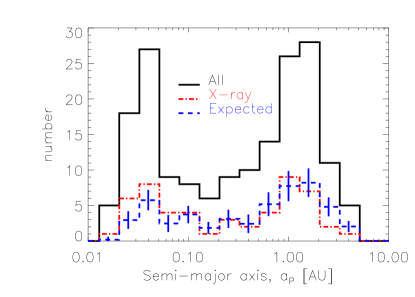
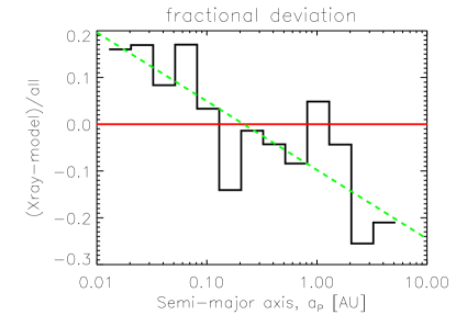
Figure 1: Distribution of observed and expected number of stars, as a function of the semi-major axis, ${a_{P}}$ of the closest planet. Left: The solid histogram represents the sample of main sequence stars among those listed in Table 2, while the dot-dashed histogram represents the subset of those stars which have been detected in X-rays. The dashed histogram with error-bars denoted by vertical line segments is the distribution generated by adopting known X-ray luminosity functions and carrying out Monte Carlo simulations for stars at the specific distances given in Table 2. Right: The histogram shows the fractional difference between the predicted and the actual number of X-ray detections in the sample. The solid horizontal line depicts the case of a perfect match, while the dashed line shows the best-fit linear fit to the residuals. This shows that there may exist a weak trend in the data towards a higher number of X-ray detections for stars that have close-in planets.

A direct comparison of these surveys with our star sample is however misleading; one must account for the intrinsic variations in X-ray luminosities and the inhomogeneous scatter in distances in our sample. To investigate this, we carry out a Monte Carlo simulation on our sample of stars, fixing each star at its given distance, but allowing their X-ray luminosities to vary. These luminosities are obtained by adopting the known X-ray luminosity functions (derived from statistically complete samples of nearby field stars using Einstein data; they thus include all the variations known to exist for coronal sources; cf. Kashyap et al. 1992). We generate 1000 realizations of X-ray fluxes at Earth using these luminosity functions for each star, and consider them to be detected in X-rays if the flux at Earth is $>2\times 10^{-13}$ ergs cm^-2 s^-1 (corresponding to the typical RASS sensitivity; Schmitt 1997). The resulting frequency distributions of imputed detections can then be compared to the observed frequency distribution of X-ray detections in our sample. This comparison is shown in Figure 1, where the frequency distributions of actual X-ray detections in our sample (dash-dotted line) and of simulated X-ray detections for a nominal set of field stars located at the same distances as the stars in our sample (dashed line, with error bars derived from averaging over the Monte Carlo realizations) are shown as a function of the planetary orbit size. Also shown are the fractional residuals between the actual and predicted number counts (solid histogram), which shows a weak trend towards a higher efficiency of detection for stars with close-in planets (dashed line; slope=$-0.1\pm 0.03$). A quantitative comparison between the two distributions yields a reduced $\chi^{2}$ of $\approx 1.8$, denoting that they are marginally statistically distinguishable.

A comparison of the X-ray luminosity distribution of the sample of stars with planets, compared to a nominally unbiased distribution from field stars is shown in Figure 2. The expected X-ray distributions are shown as the shaded region, and the actual luminosity distribution (derived as a Kaplan-Meier estimator; see e.g., Schmitt 1985, Feigelson & Nelson 1985) as the solid histogram. A formal Kolmogorov-Smirnoff test between the two shows that the null hypothesis that the data are drawn from the full sample cannot be ruled out. Most of the differences can be attributed to detections over a range of $L_{X}\sim 3\times 10^{27-28}$ ergs s^-1. While not definitive, this again suggests the need for a more sensitive analysis.

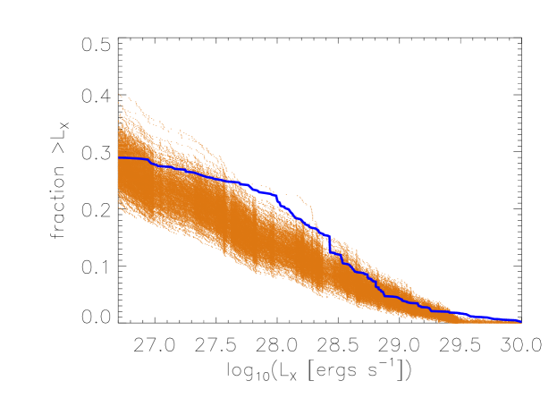
Figure 2: X-ray luminosity distribution function. The fraction of stars with a given luminosity $L_{X}$ is shown for both the main sequence sample from Table 2 (solid histogram) as well as for the expected distribution based on a model of the Galaxy (shaded region). The width of the shading represents the statistical error present, both in terms of the numbers of stars as well as the uncertainties inherent in the construction of the X-ray luminosity functions. The two cannot be statistically distinguished under a Kolmogorov-Smirnoff test.

3.2 Correlation with ${a_{P}}$

We show above (§3.1) that, taken as a whole, the set of main sequence stars with EGPs is similar in gross characteristics to, though not identical to, the field star sample. Given that, we next consider possible variations within our sample, to test whether the EGPs have any measurable effect on levels of X-ray emission. Because frequency distributions are heavily model dependent and are limited to integer values, they do not have sufficient statistical power to detect weak variations in the properties of the stars. We expect that the effect of EGPs will increase as the orbital distance decreases, and vice versa; we therefore check for direct correlations of various sample parameters with the orbital distance of the EGP.

We also note that the sample is not volume limited, and that this may introduce a number of complications into the analysis. We therefore consider an additional filter to obtain a subset of the main-sequence stars that are within 60 pc. The number distribution of these stars is uniform within this distance (see Figure 3), and this subsample comes closest to a statistically complete volume limited sample.

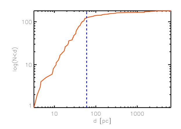
Figure 3: The distribution of the number of main-sequence star systems with distance. The cumulative number within a given distance is plotted as the solid curve. The vertical dashed line represents the distance limit of the statistically complete subsample at 60 pc, within which the star systems are uniformly distributed.

We expect a priori that tidal and magnetic effects due to close-in giant planets will manifest themselves as a trend in stellar activity as a function of the planetary orbit ${a_{P}}$. We have thus carried out detailed statistical analyses to measure correlations of the X-ray luminosity $L_{X}$ and the activity indicator $\frac{L_{X}}{L_{Bol}}$ with ${a_{P}}$. We have carried out these tests for the full sample of main-sequence star systems which have had planets detected via the Radial Velocity method, as well as for the subsample of stars which are known to be X-ray emitters, and for the subsample of stars which lie within 60 pc. If a given star has multiple planets detected, we choose the planet with the smallest semi-major axis as defining ${a_{P}}$. We compute both Pearson’s and Spearman’s Rank Correlation coefficients, and report the results in Table 3. The errors on Pearson’s coefficient are derived via bootstrapping by sampling with replacement. The significance of Spearman’s $\rho$ is denoted by the $p$-value, which measures the probability that the observed value of $\rho$ can be obtained as a chance fluctuation.

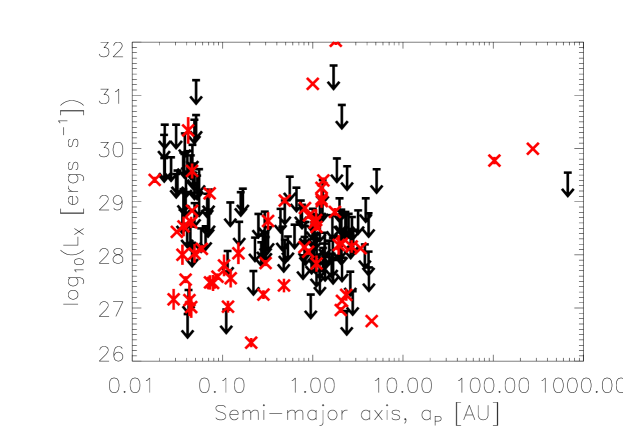
Figure 4: X-ray luminosities of the sample stars as a function of the orbital distance of the closest EGP. The downward arrows mark upper limits based on non-detections in RASS. The X-ray detections are marked with an ‘x’; the errors on the measured fluxes are denoted by vertical bars.

Table 3: Correlation of orbital semi-major axis ${a_{P}}$ with stellar parameters

Parameter	Dataset	Pearson’s Coefficient	Spearman’s $\rho$
$L_{X}$	Full sample	$-0.01\pm 0.06$	$-0.09\pm 0.05$
	X-ray detections	$-0.03\pm 0.1$	0.01 ($p=0.96$)
	volume limited	$0.02\pm 0.29$	-0.08 ($p=0.38$)
$\log_{10}\left(\frac{L_{X}}{L_{Bol}}\right)$	Full sample	$-0.04\pm 0.1$	$-0.09\pm 0.05$
	X-ray detections	$0.16\pm 0.09$	0.006 ($p=0.96$)
	volume limited	$0.26\pm 0.12$	-0.08 ($p=0.38$)
$d_{*}$	Full sample	$-0.19\pm 0.03$	-0.2 ($p=0.003$)
	X-ray detections	$-0.28\pm 0.1$	-0.07 ($p=0.6$)
	volume limited	$0.09\pm 0.06$	-0.07 ($p=0.5$)
$R_{*}$	Full sample	$-0.023\pm 0.045$	-0.05 ($p=0.47$)
	X-ray detections	$-0.05\pm 0.09$	0.10 ($p=0.48$)
	volume limited	$-0.05\pm 0.1$	0.17 ($p=0.06$)

We show the distribution of X-ray detections and upper limits for the full sample in Figure 4 as a function of ${a_{P}}$. No trend is visually discernible here in $L_{X}({a_{P}})$. Detailed correlation analysis (see Table 3) shows that there may be a slight negative correlation: for the full sample, Spearman’s Rank correlation coefficient is $\rho=-0.09\pm 0.05$ (the $1\sigma$ error bar on $\rho$ is computed via 10000 Monte Carlo simulations with the uncertainties in $L_{X}$ taken into account at each iteration). This is weakly significant, but the correlation becomes less significant when smaller samples are considered (for the X-ray detections, $\rho=0.01$, with $p=0.96$ even when uncertainties in $L_{X}$ are ignored, and for the volume limited sample, $\rho=-0.08$ with $p=0.38$). We also compute Pearson’s correlation coefficient, which uses the information of the actual values of the luminosities and not just their rank order, and thus produces statistically more powerful estimates. As before, we obtain error bars by carrying out Monte Carlo simulations that take into account the uncertainties in $L_{X}$; we adopt a Gaussian sampling function with $\sigma$ equal to the measured error for detected sources and a flat distribution in $\log{L_{X}}$ for undetected sources. We find that Pearson’s coefficient is $-0.01\pm 0.06$ for the full sample, $-0.03\pm 0.1$ for the X-ray detected sample, and $0.02\pm 0.3$ for the volume limited sample.

A similar weak correlation is found when the correlation of the activity indicator $\frac{L_{X}}{L_{Bol}}$ with ${a_{P}}$ is considered. For the set of all stars, Pearson’s coefficient is $-0.04\pm 0.11$ (Spearman’s $\rho=-0.25\pm 0.001$), for only X-ray detected stars, it is $0.16\pm 0.1$ (Spearman’s $\rho=0.01$; $p=0.96$), and for the volume limited sample, $0.26\pm 0.12$ (Spearman’s $\rho=-0.08$; $p=0.38$). We consider the activity indicator in greater detail below (see §4.1) in establishing the magnitude of the sample bias.

Since we do not expect that $L_{X}$ and ${a_{P}}$ are linearly related, and because the dynamic range is large, it is not surprising that the correlation tests are contradictory and inconclusive. A more sensitive analysis is therefore required, and we adopt a technique wherein the contrast in the data is maximized (see §3.3) by increasing the lever arm between extremal subsamples.

In addition to the X-ray luminosity $L_{X}$, we also consider the correlations of the stellar distance and stellar radius with ${a_{P}}$. We expect a negative correlation to exist with distance to the star, simply because it is easier to detect planets and activity around nearby stars. This is borne out by the correlation analysis: we find that Pearson’s coefficient is $-0.19\pm 0.03$ (Spearman’s $\rho=-0.21$, with $p=0.003$) for the entire sample, and for the X-ray detected sample alone, Pearson’s coefficient is $-0.28\pm 0.1$ (Spearman’s $\rho=-0.07$, $p=0.6$). For the volume limited sample, in contrast, we obtain a Pearson’s coefficient of $0.09\pm 0.06$ (Spearman’s $\rho=0.07$, $p=0.46$). Note that here we determine the errors via bootstrapping by sampling with replacement. We expect to find no correlation with stellar radius, and this expectation is borne out by the correlation analysis. For the full sample, Pearson’s coefficient is $-0.02\pm 0.04$ (Spearman’s $\rho=-0.05$, $p=0.47$); for the X-ray detected sample, $-0.05\pm 0.09$ ($\rho=0.1$, $p=0.48$); and for the volume limited sample, $-0.05\pm 0.1$ ($\rho=0.17$, $p=0.06$).

3.3 Extremal Subsamples

In order to clarify the variations in the X-ray activity statistically, we consider the extreme cases of stars with planets that are close to the primary (the “close-in” sample) and compare their luminosities with those of stars with planets at large distances (the “distant” sample). We choose these subsamples from the volume limited sample, i.e., main sequence star systems which are within 60 pc. This signal is obviously dependent on the contrast between the close-in and the distant samples, and in order to obtain the best contrast it is necessary to choose samples that are as far apart in their range of ${a_{P}}$ as possible and yet contain as large a sample of stars as possible. A comprehensive investigation of the best such separation is not feasible for this sample because of the large number of X-ray non-detections and the variety of tests that we carry out on the data. However, for our purposes it is sufficient to determine whether there exists subsamples which show the requisite contrast, at some separations, even if it is not necessarily the optimal one. (Note that we do consider below the effect of varying the sizes of the samples.) We therefore adopt an ad hoc separation based on the population distribution (Figure 1): we choose ${a_{P}}<0.15$ AU (corresponding to a dip in the frequency distribution of stars as a function of orbital distance ${a_{P}}$) for the close-in sample, which results in a sample size of 40 stars, 20 of which are detected in X-rays. By limiting the lower bound of the distant sample such that there is separation of an order of magnitude difference in ${a_{P}}$ between the limits of the two samples, we set for the distant sample, ${a_{P}}>1.5$ AU; 8 of 38 stars in this subsample are detected in X-rays. This range ${a_{P}}$ has the additional advantage that similar numbers of stars are found in each set. The mean X-ray luminosities for these two subsamples are found to be well separated, with the close-in sample being significantly X-ray brighter (see Figure 5). We comment on alternative choices further below (see §4.2) and explicitly show (Figure 6) that this specific choice does not affect our results.

Because of the large number of upper limits in the dataset, we cannot carry out simple hypothesis tests to verify whether these two samples are derived from the same parent distribution. Instead, we carry out Monte Carlo realizations of the sample as before (§3.2), using a Gaussian error distribution with measured errors for the detected stars and a flat uniform distribution in the log-scale for the undetected stars. We compute sample means for each set of realizations, and the distribution of these means allows us to determine whether the two samples are similar or different.

We find that the mean X-ray luminosity of the close-in sample is $<L_{X}({a_{P}}<0.15)>=10^{28.49\pm 0.09}$ ergs s^-1, and that of the distant sample is $<L_{X}({a_{P}}>1.5)>=10^{27.85\pm 0.18}$ ergs s^-1. The mean level of emission for the close-in sample is significantly greater than for the distant sample, and as shown in Figure 5, the two samples are found to be different at $>99$% confidence level.

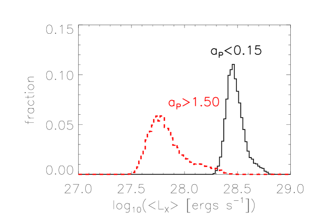
Figure 5: Mean $L_{X}$ for the extreme samples. The distribution of simulated means for the set of stars with the closest giant planet having semi-major axis ${a_{P}}<0.15$ AU is shown as the solid histogram, and its counterpart for stars that have giant planets with ${a_{P}}>1.5$ AU is shown as the dashed histogram. The overlap between the two distributions is $<1$%.

As discussed above, our choice of the limiting ${a_{P}}$ for the two subsamples is ad-hoc. We have therefore considered the effect on our result of of varying the subsample bounds of ${a_{P}}$. The mean $L_{X}$ for various subsamples is obtained using Monte Carlo simulations as above, for various ranges of ${a_{P}}$, and are shown in Figure 6. Two types of subsamples are considered: one that includes all stars with planetary orbital radii $<{a_{P}}_{close-in}$, from which the mean X-ray luminosity $<L_{X}({a_{P}}<{a_{P}}_{close-in})>$ is obtained (upper shaded curve), and another that includes all stars with orbital radii $>{a_{P}}_{distant}$, which results in $<L_{X}({a_{P}}>{a_{P}}_{distant})>$ (lower shaded curve). As can be seen, the sample that includes close-in planets is invariably more X-ray intense than the sample that includes distant planets for almost all possible choices of $<{a_{P}}_{close-in}$ and $>{a_{P}}_{distant}$. Note that these results do not change in any qualitative way if the dM stars (which contribute significantly to the high mean $L_{X}$ point at small ${a_{P}}$) are excluded from the sample.

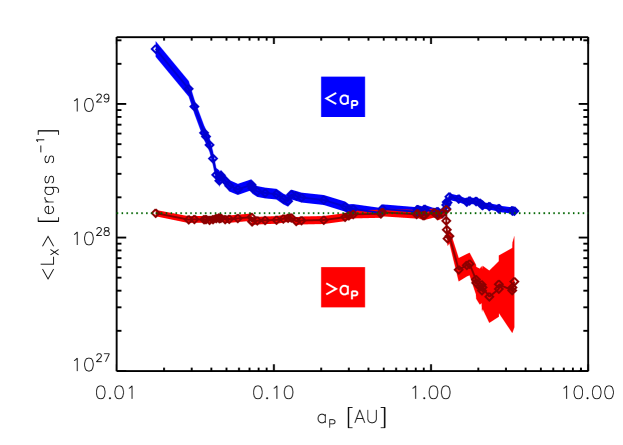
Figure 6: Comparison of mean $L_{X}$ for extremal subsamples. The width of the shading represents the $1\sigma$ statistical error on the mean $L_{X}$ derived via bootstrapping and Monte Carlo simulations (see text). The upper shaded region represents subsamples that include close-in planets, $<L_{X}({a_{P}}<{a_{P}}_{close-in})>$ and the lower shaded region, the subsamples that include distant planets $<L_{X}({a_{P}}>{a_{P}}_{distant})>$. The mean values in both cases are shown as thick dark lines marked with diamonds within the shaded regions. The distributions in Figure 5 correspond to vertical cuts across the shaded regions here, at ${a_{P}}_{close-in}=0.15$ (upper region, for $<L_{X}({a_{P}}<0.15)>$) and ${a_{P}}_{distant}=1.5$ (lower region, for $<L_{X}({a_{P}}>1.5)>$).

We caution that this observed difference in the mean $L_{X}$ between stars with close-in and distant planets cannot be entirely attributed to the effect of close-in EGPs; there are selection biases inherent in the sample that must be accounted for. By considering indirect sample ensemble properties, we argue below (see §4.1) that the bias inherent in our selected sample has a small effect. Based on physical grounds (see §§1,4.3), we expect that close-in giant planets could have a significant effect on the X-ray activity level of the primary, and the trend seen in the activity level as a function of the size of the planetary orbit (semi-major axis ${a_{P}}$) must in large part be due to the effect of the close-in giant planet.

4 Discussion

4.1 Sample Bias

The sample of candidate stars for which planet searches are conducted is subject to some subtle biases. Some of these biases have the effect of masking the signature of planet induced activity and are difficult to quantify since the planet detection processes are numerous, the programs are still incomplete, and the rates of false positives and false negatives are unknown. We may however determine the approximate extent of these biases by studying the ensemble properties of the sample of stars with detected planets. Here we describe these biases, and consider their effect on our ability to detect intrinsic trends in X-ray activity. Furthermore, because the set of EGPs is dominated by those identified with the radial velocity method, we shall limit our sample to those stars which have been verified to have planetary systems by this method, and will thus consider only those biases introduced by that method.

1. Spectral Homogeneity Most of the stars for which planets are searched for are solar like. This is advantageous to our study since the stars considered here are relatively homogeneous; therefore effects that arise due to changes in the convective turnover timescales leading to changes in the nature of the magnetic dynamo at the high- and low-mass ends of the coronal sequence, or due to the changing evolutionary states of the systems may generally be ignored. We further homogenize the sample by limiting it to main sequence stars within 60 pc (additional types of filtering to further homogenize the samples has no effect on our results; see §4.2).

   Because the sample of stars is homogeneous, we do not expect any correlations between the stellar radii $R_{*}$ and ${a_{P}}$ to be present, and indeed we find that the data are consistent with these expectations (Table 3). We have also carried out a full analysis of the extremal subsamples for various subsets of the full dataset (see Figure 10) and show that our results are robust to such selections. We thus conclude that in our sample there is no bias present due to stellar type or size effects.

2. Stellar Distance For a given planetary mass, the detectability of planets decreases as the distance of the planet from the star (${a_{P}}$) increases, since the radial velocity amplitude decreases. Since detectability in general decreases with distance to the star ($d_{*}$), we expect to find more stars with small ${a_{P}}$ at larger $d_{*}$. In the sample of stars with detected planets, we therefore expect that ${a_{P}}$ and $d_{*}$ are anti-correlated. Indeed, we find a slight negative correlation between ${a_{P}}$ and $d_{*}$, though it is weak (see Table 3). This bias exists simply as a result of the limitations of measurement statistics and is independent of any stellar activity effects. Thus, if we assume that X-ray properties of stars are independent of the distance limit, the only effect on the X-ray data will be to have a larger fraction of higher upper limits at smaller ${a_{P}}$ (due to the larger numbers of more distant stars). Thus, stellar distance should have no effect on the ensemble properties of the X-ray luminosities of stars from such a sample. In any case, we carry out most of our analysis with the volume limited sample, which is explicitly designed to remove any such effect.

3. Selecting for reduced activity The process of planet detection via the radial velocity method (RV; e.g., Butler, et al. 1996) is limited by the amount of intrinsic RV jitter that may be caused by stellar activity (Saar & Donahue 1997, Saar et al. 1998; see also Baluev 2008), and hence planets are preferentially detected when they are close-in, massive, and the primary star is not active.

   Because radial velocity signatures are hard to detect around active stars, there is a tendency to select candidate stars for planet search against activity. Thus, a priori there is an expectation that the sample of stars with detected planets would have lower activity levels than field stars of the same type. But as shown in §3.1, the X-ray emission from these stars is by and large consistent with field star emission levels. In any case, in order to avoid introducing accidental biases by comparing the sample of stars with EGPs to those without detected EGPs (note that a lack of detection does not preclude the existence of planets around the star – even if the star is part of the planet search program, there may be a planet that is less massive or more distant than the sensitivity that has been reached), we have chosen to compare the extrema of a single distribution, viz., the sample of stars known to possess giant planets. Thus any global selection effect that may exist in the sample towards lesser activity will apply equally to both subsamples and its effects are irrelevant for this study.

   Also note that in some types of planet detection methods, persistent stellar activity fixed to an active longitude can mimic the signature of a planet (Lanza et al. 2008). This results in false detections of planets at the stellar orbital period. However, this has an effect on photocentric methods and have no effect on radial velocity or transit methods currently in use.

4. Intra-sample trend in inhibition of activity If stellar activity inhibits planet detection, then it will inhibit it selectively. Planets at large ${a_{P}}$ are preferentially detected around stars with weak activity, since high activity may mask the RV signal of the distant planet. Thus, in a sample of stars selected based on the existence of planets, those stars with distant planets are presumptively less active. This bias thus produces the same signature in activity trends that we search for (see §3.3), and thus interferes with our study.

   How can this bias be quantified? Consider that the cause of the bias is the excess jitter in velocity induced by magnetic activity, which is related to the energy deposited in the corona, which in turn is tracked by the ratio of X-ray to bolometric luminosity $\frac{L_{X}}{L_{Bol}}$. This jitter serves to mask the RV signal, which is due to wobble from gravitational effects and is therefore inversely proportional to the orbital semi-major axis of the planet. Thus, the bias will manifest itself as a positive correlation between the formally independent parameters $\frac{L_{X}}{L_{Bol}}$ and $\frac{1}{{a_{P}}}$. Note that this correlation is not necessarily linear because it is dependent on the observation process, the cumulative observation time, etc. Any existing correlation also does not imply causality, and indeed the velocities that are generated by these two processes are quite different. Nevertheless, we expect that stars with large values of $\frac{L_{X}}{L_{Bol}}$ will primarily be present in our sample provided they are also accompanied by small values of ${a_{P}}$. Thus, a measurement of the correlation between these two variables serves as a measurement of the sample bias. For the sample of main sequence stars within 60 pc that have EGPs detected via the RV method, we find that

   $$\log_{10}\frac{L_{X}}{L_{Bol}}=(-5.65\pm 0.04)+(0.22\pm 0.05)\cdot\log_{10}\frac{1}{{a_{P}}}\,,$$ (2)

   where ${a_{P}}$ is in units of [AU]. Here the errors are derived via Monte Carlo bootstrapping on the X-ray flux measurement errors. Thus, we find that there does exist a weak, but statistically significant, correlation between $\frac{L_{X}}{L_{Bol}}$ and $\frac{1}{{a_{P}}}$. This trend is shown in Figure 7. Conservatively assuming that all of this correlation is attributable to the inherent bias, we can then estimate its effect on the observed activity trend. That is, for each of the stars in the close-in and distant samples (in §3.3), given ${a_{P}}$ and $L_{Bol}$ we can compute a predicted $L_{X}({a_{P}},L_{Bol})$ that can then be used in the place of the measured $L_{X}$ to carry out the same analysis. The result of this calculation is shown in Figure 8, which shows that the close-in and distant samples differ by $\approx{1}\sigma$, and account for only a factor of $\sim 2$ of the observed difference between the two samples. It is important to note that the magnitude of this bias will vary for every subsample, and that the magnitude and direction of the bias will be case specific.

   

   
   

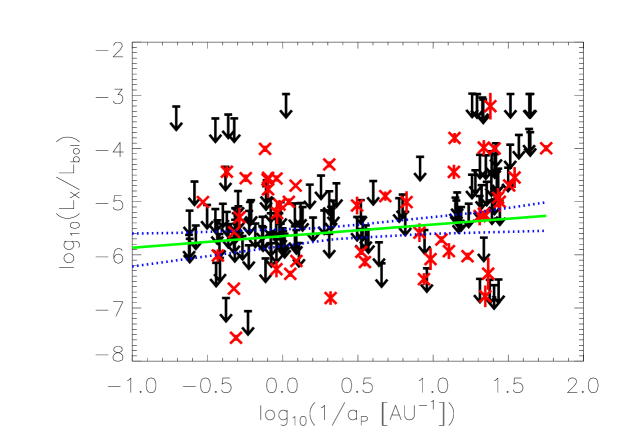
   Figure 7: The distribution of $\log\frac{L_{X}}{L_{Bol}}$ with $\log\frac{1}{{a_{P}}}$. The X-ray detections are marked with ‘x’s, with error bars denoted with vertical lines; the X-ray non-detections are shown with downward arrows. Also shown are the best-fit regression line (solid curve) and the envelope bound of the bootstrapped regression curves (dotted lines). Since more active stars have higher radial velocity jitter, we expect fewer planets to be detected around stars at high $\frac{L_{X}}{L_{Bol}}$ unless they also have high $\frac{1}{{a_{P}}}$; this correlation tracks an important sample bias (see text). This trend is removed from the rest of the analysis.

   

   
   

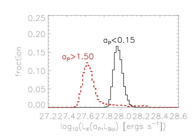
   Figure 8: Same as Figure 5, but using $L_{X}({a_{P}},L_{Bol})$ estimated from the regression analysis on $\frac{L_{X}}{L_{Bol}}$ with $\frac{1}{{a_{P}}}$ (Equation 2). The two distributions differ by $\approx{2}\sigma$.

   Note that $\frac{L_{X}}{L_{Bol}}$ is the preferred proxy for activity because it is surface area independent. However, because there are no $R_{*}$ biases in the sample, $L_{X}$ and $\frac{L_{X}}{L_{Bol}}$ are similarly correlated with ${a_{P}}$. Thus, a priori, we expect that accounting for the selective inhibition bias of Equation 2 in the ${a_{P}}$ vs $L_{X}$ dataset should result in a complete removal of any luminosity difference between the extremal samples, i.e., that $\frac{<L_{X}({\rm close-in}>}{<L_{X}{\rm distant}>}\approx 1$. That this is manifestly not so (Figure 9) is an indication that the differences in the distribution of $L_{X}$ for the extremal samples is systematic, and an inherent property of the observed sample.

   Furthermore, the bias measurement is conservative, i.e., we include some of the desired signal within the estimate of the bias, and thus we overestimate the magnitude of the bias. Because this bias is removed from the observed ratios of the mean luminosities, our results provide a conservative estimate of the true magnitude of the effect of planet-induced activity.

5. Intrinsic sample variance Other parameters known to affect the level of stellar activity are age, rotation, the Rossby number, metallicity, temporal variability, etc.

   Stellar ages are not known with sufficient accuracy for us to consider them here, and it is possible that there exists a trend where ${a_{P}}$ is correlated with stellar age. But note that such hidden variables do not affect the results derived here, and simply point to a more complex explanation of the connection between close-in planets and stellar activity.

   It is also as yet unclear what type of effect a massive Jupiter-type planet will have on these parameters. For instance, Rotational synchronization by tidal interactions may be thought to increase $v\sin{i}$ and thereby coronal activity for close-in EGPs compared to distant EGPs. However, not only is this as likely to spin-down a fast rotating star as to spin-up a slow-rotator, but also the timescales for the synchronization of the stellar rotation period with the planetary orbital period are very large to begin with, and increase as ${a_{P}}^{6}$ for distant planets (see e.g., Drake et al. 1998 and references therein), implying that most stars in the sample are not synchronized to the orbits of their close-in giant planets. We therefore conclude that both theoretical and observational prejudice points to evenly scattered values for these stellar parameters in our sample.

4.2 Activity Enhancement

We use the parameterization of the bias described above (see §4.1) to determine the residual signal, i.e., the magnitude of the excess X-ray activity in the close-in subsample compared to the distant subsample that can be attributed to the effect of EGPs. In order to simplify the calculation, we consider the ratio of the average luminosities of the close-in and distant subsamples calculated during the Monte Carlo simulation described above (see analysis in §3.3). The data from Figure 5 are shown as the solid histogram in Figure 9, and confirm that the close-in subsample is on average more X-ray luminous by a factor $4^{<7}_{>2.8}$, where the bounds on the number indicate the extent of the asymmetrical $1\sigma$-equivalent errors. After correcting for the sample bias (by dividing the original ratio by the ratio of the luminosities as predicted by Equation 2), we find that the bias-corrected luminosity ratio decreases, but is $>1$ at a significance of $0.95$. This constitutes a definite detection of activity enhancement, by a factor $2.3^{<4}_{>1.3}$ (dashed histogram in Figure 9). This remaining enhancement can be attributed to the effect of close-in giant planets on their parent stars. We therefore conclude that the close-in and distant samples indeed show differing X-ray activity levels and that a factor $\sim 2$ can be attributed to the effect of close-in EGPs. Note that the existence of this residual enhancement does not in itself allow us to conclude that there is a causal connection between the closeness of giant planets to their primary stars and the activity levels on those stars. However, in conjunction with the Ca II HK enhancements observed by Shkolnik et al. 2003), our results suggest that such a connection may be present.

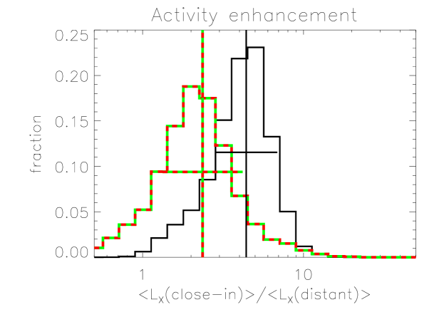
Figure 9: Distributions of $<L_{X}{\rm(close-in)}>/<L_{X}{\rm(distant)}>$. The distribution of the ratios of simulated $L_{X}$ for the close-in (${a_{P}}<0.15$ AU) and distant (${a_{P}}>1.5$ AU) samples is shown as the solid histogram. The same ratios, modified to account for the sample bias (see §4.1) are shown with dashed lines. The means and standard deviations of the two distributions are denoted with vertical and horizontal lines respectively (solid and dashed, for the two distributions). The data show that the two extremal samples differ by a factor $\approx{4}$ (between 2.8 to 7 times), and after sample bias is accounted for, by a factor $\approx{2}$ (between 1.3 and 4 times).

As a further check on the sensitivity of our analysis to the samples used, we compute the same ratio as in Figure 9 for a number of different subsamples. The resulting distributions of the ratios of mean luminosity for close-in versus distant subsamples are shown in Figure 10; in all cases the close-in subsamples have larger $<L_{X}>$ than the distant subsamples.

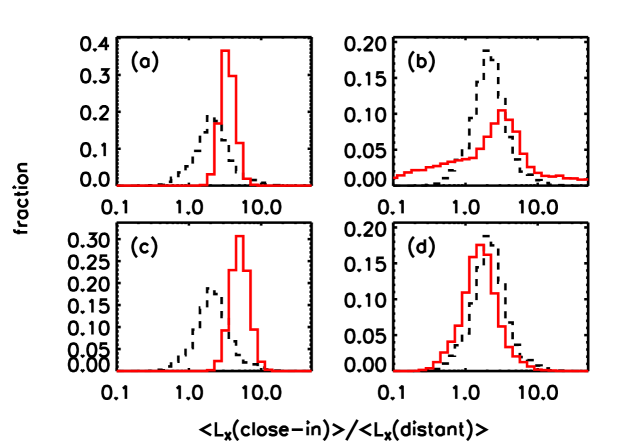
Figure 10: Effect of variations of sample composition on the distribution of $<L_{X}{\rm(close-in)}>/<L_{X}{\rm(distant)}>$. The ratios of $<L_{X}({a_{P}}<0.15)>/<L_{X}({a_{P}}>1.5)>$ are compared for different representative subsets of the full sample of stars with detected planets. In all plots, the baseline comparison from Figure 9, for the main-sequence sample within 60 pc, is shown as the dashed histogram. The solid histograms are: (a) all X-ray detections, (b) the full sample of all stars with EGPs detected via the RV method, (c) the nearby main-sequence sample excluding dM stars, and (d) the full sample as in (b), excluding giants. In all cases, the bias correction (see §4.1) is done separately for each sample. In all cases, the evidence is strong that stars with close-in giant planets are more active than those with distant planets.

Note that the above result is dependent on the bounds chosen for ${a_{P}}$ for both subsamples. Clearly, the contrast between the two extremal sets would be heightened if the range of ${a_{P}}$ defining the two subsamples is shrunk further, and vice versa. This must also be balanced by the decreased robustness of the result due to the consequent dearth of X-ray detections in the subsamples. A rigorous estimate of the “best” split between the close-in and the distant samples is not feasible because of the large number of stars that remain undetected in X-rays and the need to compute the bias factor (Equation 2) separately for each case. Nevertheless, as we have shown above (Figure 6) there exists a persistent difference in the mean luminosity between the close-in and distant subsamples, and it favors the suggestion that stars with close-in planets tend to be more active. The best way to improve this result is to obtain X-ray detections of more stars at the extreme ranges of ${a_{P}}$.

4.3 Dependence of the X-ray excess on ${a_{P}}$

For tidally interacting close binaries in a sample that included RS CVn stars, Schrijver & Zwaan (1991) found that the X-ray surface flux $F_{X}\propto\sqrt{a_{*}}$, where $a_{*}$ is the distance to the cooler component. Comparing the average X-ray luminosities for close-in and distant subsamples that we derive above (see §§3.3,4.2), after sample biases have been corrected for, we find that

$$<F_{X_{\rm corr}}>~{}~{}\propto~{}~{}<{a_{P}}>^{-0.35\pm 0.17}\,,$$ (3)

which is a smaller dependence than that found by Schrijver & Zwaan, but the large error bar prevents a definitive conclusion.

It is well known that binary stars are generally more X-ray active than single stars of the same type and rotation rate (see, e.g., Zaqarashvili, Javakishvili, & Belvedere 2002 and references therein). Numerous mechanisms have been proposed to account for this so-called “overactivity,” generally based on tidal and magnetic interactions. These studies were extended to the case of stars with EGPs and brown dwarfs by Cuntz et al. (2000). They suggested that the energy generation due to tidal interactions is proportional to the gravitational perturbation

$$\frac{\Delta g_{*}}{g_{*}}=\frac{M_{P}}{M_{*}}\frac{2R_{*}^{3}}{({a_{P}}-R_{*})^{3}}$$ (4a)

where $$M_{*} M_{P}$$ is the mass of the star and that of the EGP, and the height of the tidal bulge,

$$h_{tide} \propto \frac{\Delta g_{*}}{g_{*}}R_{*}$$ (4b)

$$\propto \frac{M_{P}}{M_{*}}R_{*}^{4}{a_{P}}^{-3}$$

$$\propto {a_{P}}^{-3}\,.$$

Saar et al. (2004) estimated the energy released via reconnection during an interaction of the planetary magnetosphere with the stellar magnetic field,

$$F_{int} \propto B_{*}B_{P}v_{rel}{a_{P}}^{-n}$$ (5)

$$\propto {a_{P}}^{-n}\,,$$

where $B_{*}$ and $B_{P}$ are the stellar and planetary magnetic fields, $v_{rel}$ is the relative velocity between them that produces the shear in the magnetic fields and leads to the reconnection. Here, $n=3$ very close to the star and $n=2$ farther away (in the “Parker spiral”). Thus, if the magnitude of the enhancement and the stellar magnetic field can be measured for these systems, then the planetary magnetic environment can be investigated.

Since our measurements are an ensemble average, i.e., they do not take into account variations in mass, magnetic fields, and relative velocities, we cannot directly verify the above models. Nevertheless, we can obtain a rough estimate for the variation of the “excess” luminosity with ${a_{P}}$ by assuming that

$$\delta{L_{X}}\propto{a_{P}}^{x}$$ (6)

where $\delta{L_{X}}$ is the difference between the actual luminosity and a luminosity unaffected by a close-in EGP. For the former, we use the values simulated during the Monte Carlo analysis of §3.3, and approximate the latter with the average $L_{X}$ derived for the distant sample. Fitting straight lines to $\log{\delta{L_{X}}}$ vs $\log{{a_{P}}}$, and accounting for the bias in the same manner as described above in §4.2, we find that $x\approx{-1}$. The error on this value is however very large ($\sim 100\%$). Therefore, we conclude that while the data are qualitatively consistent with the scenarios proposed by Cuntz et al. (2000), a reliable test of the theory is not feasible without more observations.

5 Summary

We have searched for X-ray emission from a sample of 230 stars with known giant planets with a view to characterizing the effect of the EGPs on the parent star. We first find that the overall sample of stars with known EGPs is similar in gross X-ray properties to field star samples (see §3.1), and thus provides a representative sample of X-ray stars. We carry out a careful search for statistical trends with various parameters (see §3.2) and find some evidence that the activity levels of stars with close-in giant planets is higher than for stars with planets located further out, though the correlations are contradictory and inconclusive. We then carry out a more powerful test by analyzing in detail two extremal subsamples (see §3.3) where we compare the X-ray emission from nearby (distance$<$60 pc) main-sequence stars with close-in EGPs against similar stars with much more distant EGPs. For the sake of definiteness, we choose a close-in sample where the orbital semi-major axis ${a_{P}}<0.15$ AU, and a distant sample where ${a_{P}}>1.5$ AU (reducing the separation between the samples increases the number of stars considered, but reduces the contrast between the samples). We verify that our adopte ranges of ${a_{P}}$ are not special by varying the limiting ranges of ${a_{P}}$ over which the subsamples are defined, and find that invariably the close-in samples have X-ray luminosities higher than that of the distant sample.

The above result must be understood in the context of selection biases in our sample of stars. In §4.1, we demonstrate that observational biases account for about half of the observed differences seen in the data. After these biases are accounted for, we find that the close-in sample is more active by a factor of $2_{>1.3}^{<4}$ on average. This result holds even when the full data are filtered with different selection criteria.

The robustness of the result is limited by the large number of systems yet to be detected in X-rays. New observations by Chandra or XMM-Newton would consequently improve the statistics and would constrain the magnitude of this effect with better precision. We note that a simple model of the X-ray emission enhancement suggests an interaction strength proportional to the product of the stellar and planetary magnetic fields, $B_{*}\,B_{P}$ at their point of interaction. This suggests that if $B_{*}$ is known or can be estimated, $B_{P}$ for exoplanets can potentially be studied. Since the point of interaction between $B_{P}$ and $B_{*}$ depends in part on the strength of the stellar wind, close-in wind properties can also potentially be probed by such observations.

References

- (1)
- (2) Anderson, D., et al., 2008, MNRAS, submitted
- (3) Ayres, T.R., Fleming, T.A., Simon, T., et al. 1995, ApJS, 96, 223
- (4) Bakos, G., Noyes, R., Kovácz, G., Latham, D., Sasselov, D., Torres, G., Fischer, D., Stefanik, R., Sato, B., Johnson, J., Pál, A., Marcy, G., Butler, P., Esquerdo, G., Stanek, K., Lázár, J., Papp, I., Sari, P., & Sipöcz, B., 2006, ApJ, accepted
- (5) Bakos, G., Shporer, A., Pal, A., Torres, G., Kovacs, G., Latham, D., Mazeh, T., Ofir, A., Noyes, R., Sasselov, D., Bouchy, F., Pont, F., Queloz, D., Udry, S., Esquerdo, G., Sipocz, B., Kovacs, G., & Lazar, J., 2007, ApJ, 671, L173
- (6) Baluev, R.V., 2008, arXiv:0712.3862, submitted to MNRAS
- (7) Barge, P., Baglin, A., Auvergne, M., & The CoRoT Team, 2007, in EXOPLANETS: Detection, Formation and Dynamics Proceedings, IAU Symposium 249
- (8) Bastian, T.S., Dulk, G.A., & Leblanc, Y., 2000, ApJ, 545, 1058
- (9) Biller, B., Kasper, M., Close, L., Brandner, W., & Kellner, S., 2006, ApJ, accepted
- (10) Bonfils, X., Forveille, T., Delfosse, X., Udry, S., Mayor, M., Perrier, C., Bouchy, F., Pepe, F., Queloz, D., & Bertaux, J.-L., 2005, A&A, 443, L15
- (11) Bouchy, F., Pont, F., Santos, N., Melo, C., Mayor, M., Queloz, D., & Udry, S., 2004, A&A, 421, L13
- (12) Bouchy, F., Pont, F., Melo, C., Santos, N.C., Mayor, M., Queloz, D., & Udry, S., 2005a, A&A, 431, 1105
- (13) Bouchy, F., Udry, S., Mayor, M., Moutou, C., Pont, F., Iribarne, N., da Silva, R., Llovaisky, S., Queloz, D., Santos, N.C., Segransan, D., & Zucker, S., 2005b, A&A, 444, L15
- (14) Burke, Ch., et al., 2007, ApJ, 671, 2115
- (15) Butler, P., Marcy, G., Vogt, S., Fischer, D., Henry, G., Laughlin, G., & Wright, J., 2003, ApJ, 582, 455
- (16) Butler, P., Tinney, C., Marcy, G., Jones, H., Penny, A., & Apps, K., 2001, ApJ, 555, 410
- (17) Butler, P., Vogt, S., Marcy, G., Fischer, D., Henry, G., & Apps, K., 2000, ApJ, 545, 504
- (18) Butler, P., Vogt, S., Marcy, G., Fischer, D., Wright, J., Henry, G., Laughlin, G., & Lissauer, J., 2004, ApJ, 617, 580L
- (19) Butler, P., Wright, J., Marcy, G., Fischer, D., Vogt, S., Tinney, Ch., Jones, H., Carter, B., & Penny, A., 2006a, ApJ, 646, 505
- (20) Butler, R.P., Johnson, J.A., Marcy, G.W., Wright, J.T., Vogt, S.S., & Fischer, D.A., 2006b, PASP, 118
- (21) Butler, R.P., Marcy, G.W., Vogt, S.S., & Apps, K., 1998, PASP, 110, 1389
- (22) Butler, R.P., Marcy, G.W., Williams, E., Hauser, H., & Shirts, P., 1997, ApJ, 474, L115
- (23) Butler, R.P., Marcy, G.W., Williams, E., McCarthy, C., Dosanjh, P., & Vogt, S.S., 1996, PASP, 108, 500
- (24) Butler, R.P., & Marcy, G.W., 1996, ApJ, 464, L153
- (25) Béjar, V.J.S., Zapatero Osorio, M.R., Pérez-Garrido, A., Álvarez, C., Martín, E.L., Rebolo, R., Villé-Pérez, I., & Díaz-Sánchez, A., 2008, ApJ, 673, L185
- (26) Campbell, B., Walker, G., & Yang, S., 1988, ApJ, 331, 902
- (27) Carter, B., Butler, P., Tinney, C., Jones, H., Marcy, G., Fischer, D., McCarthy, C., & Penny, A., 2003, ApJ, 593, L43
- (28) Charbonneau, D., Brown, T.M., Latham, D.W., Mayor, M., 2000, ApJ, 529, L45
- (29) Chauvin, G., Lagrange, A.-M., Dumas, C., Zuckerman, B., Mouillet, D., Song, I., Beuzit, J.-L., & Lowrance, P., 2005, A&A, 438, L25
- (30) Chauvin, G., Lagrange, A.-M., Dumas, C., Zuckerman, B., Mouillet, D., Song, I., Beuzit, J.-L., & Lowrance, P., 2005a, A&A, 438, L25
- (31) Chauvin, G., Lagrange, A.-M., Zuckerman, B., Dumas, C., Mouillet, D., Song, I., et, al., 2005, A&A, 438, L29
- (32) Chauvin, G., Lagrange, A.-M., Zuckerman, B., Dumas, C., Mouillet, D., Song, I., et, al., 2005b, A&A, 438, L29
- (33) Cochran, W., Endl, M., Wittenmyer, R., & Bean, J., 2007, ApJ, 665, 1407
- (34) Cochran, W., Endl, M., McArthur, B., Paulson, D., Smith, V., MacQueen, Ph., Tull, R., Good, J., Booth, J., Shetrone, M., Roman, B., Odewahn, S., Deglman, F., Graves, M., Soukup, M., & Villarred, Jr.,M., 2004, ApJ, 611, 133
- (35) Cochran, W., Hatzes, A., Butler, P., & Marcy, G., 1997, ApJ, 483, 457
- (36) Cochran, W., Hatzes, A., Endl, M., Paulson, D., Walker, G., Campbell, B., & Yang, S., 2002, BAAS, 34, 42.02
- (37) Collier-Cameron, A., Bouchy, F., Hebrard, G., Maxted, P., Pollaco, D., Pont, F., Skillen, I., Smalley, B., Street, R., West, R., Wilson, D., Aigrain, S., Christian, D., Clarkson, W., Enoch, B., Evans, A., Fitzsimmons, A., Gillon, M., Haswell, C., Hebb, L., Hellier, C., Hodgkin, S., Horne, K., Irwin, J., Kane, S., Keenan, F., Loeillet, B., Lister, T., Mayor, M., Moutou, C., Norton, A., Osborne, J., Parley, N., Queloz, D., Ryans, R., Triaud, A., Udry, S., & Wheatley, P. , 2007, MNRAS, 375, 971
- (38) Cranmer, S.R., & Saar, S.H., 2006, at the 14th Workshop on Cool Stars, Stellar System, and the Sun, Pasadena, Nov 6-10, #160
- (39) Cuntz, M., Saar, S.H., Musielak, Z.E. 2000, ApJ, 533, L151
- (40) Cuntz, M., & Shkolnik, E. 2002, Astron.Nachrichten, 323, 387
- (41) da Silva, R., Udry, S., Bouchy, F., Mayor, M., Moutou, C., Pont, F., Queloz, D., Santos, N., Segransan, D., & Zucker, S., 2005, A&A, 446, 717
- (42) Delfosse, X., Forveille, T., Mayor, M., Perrier, C., Naef, D., & Queloz, D., 1998, A&A, 338, L67
- (43) Desidera, S., Gratton, R., Endl, M., Barbieri, M., Claudi, R., Cosentino, R., Lucatello, S., Marzari, F., & Scuderi, S., 2003, A&A, 405, 207
- (44) Doellinger, M., Hatzes, A., Pasquini, L., Guenther, E., Hartmann, M., Girardi, L., & Esposito, M., 2007, A&A, 472, 649
- (45) Drake, S.A., Pravdo, S.H., Angelini, L., & Stern, R.A., 1998, AJ, 115, 2122
- (46) Eggenberger, A., Mayor, M., Naef, D., Pepe, F., Queloz, D., Santos, N., Udry, S., & Lovis, C., 2006, A&A, 447, 1159
- (47) Endl, M., Cochran, W., Wittenmyer, R., & Boss, A., 2007, ApJ, 673, 1165
- (48) Feigelson, E., & Nelson, P., 1985, ApJ, 293, 192
- (49) Fischer, D., Laughlin, G., Marcy, G., Butler, P., & Vogt, S., 2006, in “Tenth Anniversary of 51 Peg-b: Status and Prospect of hot Jupiter Studies.” Ed L. Arnold, F. Bouchy, & C. Moutou. Platypus Press
- (50) Fischer, D., Marcy G., Butler P., Sato B., Vogt S., Robinson, S., Laughlin G., Henry G., Driscoll P., Takeda G., Wright J., & Johnson J., 2007, ApJ, submitted
- (51) Fischer, D., Butler, P., Marcy, G., Vogt, S., & Henry, G., 2003, ApJ, 590, 1081
- (52) Fischer, D., Laughlin, G., Marcy, G., Butler, P., Vogt, S., Johnson, J., Henry, G., McCarthy, Ch., Ammons, M., Robinson, S., Strader, J., Valenti, J., McCullogh, P., Charbonneau, D., Haislip, J., Knutson, H., Reichart, D., McGee, P., Monard, B., Wright, J., Ida, S., Sato, B., & Minniti, D., 2005, ApJ, 637, 1094
- (53) Fischer, D., Marcy, G., Butler, P., Vogt, S., Frink, S., & Apps, K., 2000, ApJ, 551, 1107
- (54) Fischer, D., Marcy, G., Butler, P., Vogt, S., Henry, G., Pourbaix, D., Walp, B., Misch, A., & Wright, J., 2002a, ApJ, 586, 1394
- (55) Fischer, D., Marcy, G., Butler, P., Vogt, S., Walp, B., & Apps, K., 2002b, PASP, 114 529
- (56) Fischer, D.A., Marcy, G.W., Butler, R.P., Vogt, S.S., & Apps, K., 1999, PASP, 111, 50
- (57) Frink, S., Mitchell, D., Quirrenbach, A., Fischer, D., Marcy, G., & Butler, P., 2002, ApJ, 576, 478
- (58) Galland, F., Lagrange, A.-M., Udry, S., Chelli, A., Pepe, F., Beuzit, J.-L., & Mayor, M., 2005, A&A, 444, L21
- (59) Gaudi, S., Bennett, D., Udalski, A., Gould, A., Christie, G., et al., 2008, Science, 319, 927
- (60) Ge, J., van Eyken, J., Mahadevan, S., Dewitt, C., Kane, S., Cohen, R., van den Heuvel, A., Fleming, S., Guo, P., Henry, G., Schneider, D., Ramsey, L., Wittenmyer, R., Endl, M., Cochran, W., Ford, E., Martin, E., Israelian, G., Valenti, J., & Montes, D., 2006, ApJ, 648, 683
- (61) Griessmeier, J.-M., Zarka, P., & Spreeuw, H., 2007, A&A, 475, 359
- (62) Harris, D.E., Forman, W., Gioa, I.M., Hale, J.A., Harnden, F.R.,Jr., Jones, C., Karakashian, T., Maccacaro, T., McSweeney, J.D., Primini, F.A., Schwarz, J., Tananbaum, H.D., & Thurman, J., SAO HEAD CD-ROM Series I (Einstein), Nos 18-36
- (63) Hatzes, A., Günther, E., Endl, M., Cochran, W., Döllinger, M., & Bedalov, A., 2005, A&A, 437, 743
- (64) Hünsch, M., Schmitt, J.H.M.M., & Voges, W., 1998, A&AS, 132, 155
- (65) Joergens, V., & Mueller, A., 2007, ApJ, 666, L113
- (66) Johns-Krull, C., et al., 2007, ApJ, submitted
- (67) Johnson, J., Butler, P., Marcy, G., Fischer, D., Vogt, S., Wright, J., & Peek, C., 2007a, ApJ, accepted
- (68) Johnson, J., et al., 2007b, ApJ, 675, 784
- (69) Johnson, J.A., Marcy, G.W., Fischer, D.A., Henry, G.W., Wright, J.T., Isaacson, H., & McCarthy, C., 2006a, ApJ, 652, 1724
- (70) Johnson, J.A., Marcy, G.W., Fischer, D.A., Laughlin, G., Butler, R.P., Henry, G.W., Valenti, J.A., Ford, E.B., Vogt, S.S., & Wright, J.T., 2006b, ApJ, 647, 600
- (71) Jones, H., Butler, P., Tinney, C., Marcy, G., Penny, A., McCarthy, C., Carter, B., & Pourbaix, D., 2001, MNRAS, 333, 871
- (72) Jones, H., Butler, P., Tinney, C., Marcy, G., Penny, A., McCarthy, C., & Carter, B., 2002, MNRAS, 341, 948
- (73) Jones, H.R.A., Butler, R.P., Tinney, C.G., Marcy, G.W., Carter, B.D., Penny, A.J., McCarthy, C., & Bailey, J.B., 2006, MNRAS, 369, 249
- (74) Kashyap, V., Rosner, R., Micela, G., Sciortino, S., Vaiana, G.S., & Harnden, F.R., Jr., 1992, ApJ, 391, 684
- (75) Kim, D.-W., Cameron, R.A., Drake, J.J., Evans, N.R., Freeman, P., Gaetz, T.J., Ghosh, H., Green, P.J., Harnden, F.R.,Jr., Karovska, M., Kashyap, V., Maksym, P.W., Ratzlaff, P.W., Schlegel, E.M., Silverman, J.D., Tananbaum, H.D., Vikhlinin, A.A., Wilkes, B.J., & Grimes, J.P., 2004, ApJ, accepted
- (76) Konacki, M., 2005, Nature, 436, 220
- (77) Konacki, M., Torres, G., Jha, S., & Sasselov, D.D., 2003, Nature, 421, 507
- (78) Konacki, M., Torres, G., Sasselov, D., Pietrzynski, G., Udalski, A., Jha, S., Ruiz, M.-T., Gieren, W., & Minniti, D., 2004, ApJ, 609, L37
- (79) Korzennik, S., Brown, T., Fischer, D., Nisenson, P., & Noyes, R., 2000, ApJ, 533, L147
- (80) Kovacs, G., Bakos, G., Torres, G., Sozzetti, A., Latham, D., Noyes, R., Butler, P., Marcy, G., Fischer, D., Fernandez, J., Esquerdo, G., Sasselov, D., Stefanik, R., Pal, A., Lazar, J., & Sari, P., 2007, ApJ, 670, L41
- (81) Kurster, M., Endl, M., Els, S., Hatzes, A., Cochran, W., Dobereiner, S., & Dennerl, K., 2000, A&A, 353, L33
- (82) Lanza, A.F., 2008, arXiv:0805.3010
- (83) Lanza, A.F., De Martino, C., & Rodonò, M., 2008, New Astronomy, 13, 77
- (84) Latham, D.W., Stefanik, R.P., Mazeh, T., Mayor, M., & Burki, G., 1989, Nature, 339, 38
- (85) Lo Curto, G., Mayor, M., Clausen, J., Benz, W., Bouchy, F., Lovis, C., Moutou, C., Naef, D., Pepe, F., Queloz, D., Santos, N., Sivan, J.-P., Udry, S., Bonfils, X., Delfosse, X., Mordasini, C., Fouque, P., Olsen, E., & Pritchards, J., 2006, A&A, 451, 345
- (86) Lovis, C., Mayor, M., Pepe, F., Alibert, Y., Benz, W., Bouchy, F., Correia, A.C.M., Laskar, J., Mordasini, C., Queloz, D., Santos, N.C., Udry, S., Bertaux, J.-L., & Sivan, J.-P., 2006, Nature, 441, 305
- (87) Lovis, C., Mayor, M., Pepe, F., Queloz, D., Santos, N., Sosnowska, D., Udry, S., Benz, W., Bertaux, J.-L., Bouchy, F., Mordasini, C., & Sivan, J.-P., 2005, A&A, 437, 1121
- (88) Lovis, C., & Mayor, M., 2007, A&A, 472, 657
- (89) Mandushev, G., O’Donovan, F.T., Charbonneau, D., Torres, G., Latham, D.W., Bakos, G.A., Dunham, E.W., Sozzetti, A., Fernandez, J.M., Esquerdo, G.A., Everett, M.E., Brown, T.M., Rabus, M., Belmonte, J.A., & Hillenbrand, L.A., 2007, ApJ, 667
- (90) Marchi, S., 2007, ApJ, 666, 475
- (91) Marcy, G.W., Butler, R.P., Vogt, S.S., Fischer, D., & Liu, M., 1999, ApJ, 520, 239
- (92) Marcy, G.W., Butler, R.P., Vogt, S.S., Fischer, D.A., Henry, G.W., Laughlin, G., Wright, J.T., & Johnson, J.A., 2005, 619, 570
- (93) Marcy, G.W., Butler, R.P., & Vogt, S.S., 2000, ApJ, 536, L43
- (94) Marcy, G.W., Cochran, W.D., & Mayor, M., 2000, in “Protostars and Planets IV,” Ed. V.Mannings, A.P.Boss, & S.S.Russell (Tucson: Univ.Arizona Press), 1285
- (95) Marcy, G.W., & Butler, R.P., 1996, ApJ, 464, L147
- (96) Mayor, M., Pepe, F., Queloz, D., Bouchy, F., Rupprecht, G., Lo Curto, G.. Avila, G., Benz, W., Bertaux, J.-L., Bonfils, X., Dall, Th., Dekker, H., Delabre, B., Eckert, W., Fleury, M., Gilliotte, G., Gojak, D., Guzman, J., Kohler, D., Lizon, J.-L., Longinotti, A., Lovis, C., Migevand, D., Pasquini, L., Reyes, J., Sivan, J.-P., Sosnowska, D., Soto, R., Udry, S., Van Kesteren, A., Weber, L. & Weilenmann, U., 2003, Setting new standards with HARPS, in The ESO Messenger, 114, 20
- (97) Mayor, M., Pepe, F., Queloz, D., Bouchy, F., Rupprecht, G., Lo Curto, G.. Avila, G., Benz, W., Bertaux, J.-L., Bonfils, X., Dall, Th., Dekker, H., Delabre, B., Eckert, W., Fleury, M., Gilliotte, G., Gojak, D., Guzman, J., Kohler, D., Lizon, J.-L., Longinotti, A., Lovis, C., Migevand, D., Pasquini, L., Reyes, J., Sivan, J.-P., Sosnowska, D., Soto, R., Udry, S., Van Kesteren, A., Weber, L., & Weilenmann, U., 2003a, Setting new standards with HARPS, in The ESO Messenger, 114, 20
- (98) Mayor, M., Udry, S., Naef, D., Pepe, F., Queloz, D., Santos, N.C., & Burnet, M. 2003b, A&A, 415, 391
- (99) Mayor, M., & Queloz, D., 1995, Nature, 378, 355
- (100) McCarthy, C., Butler, P., Tinney, C., Jones, H., Marcy, G., Carter, B., Penny, A., & Fischer, D., 2004, ApJ, 617, 575
- (101) McCullough, P.R., Stys, J.E., Valenti, J.A., Johns-Krull, C.M., Janes, K.A., Heasley, J.N., Bye, B.A., Dodd, C., Fleming, S.W., Pinnick, A., Bissinger, R., Gary, B.L., Howell, P.J., & Vanmunster, T., 2006, ApJ, 648, 1228
- (102) McIvor, T., Jardine, M., & Holzwarth, V., 2006, MNRAS, 367, L1
- (103) Melo, C., Santos, N., Gieren, W., Pietrzynski, G., Ruiz, M., Sousa, S., Bouchy, F., Lovis, C., Mayor, M., Pepe, F., Queloz D., da Silva, R., & Udry, S., 2007, A&A, 467, 721
- (104) Mitchell, D., Frink, S., Quirrenbach, A., Fischer, D., Marcy, G., & Butler, P., 2003 BAAS, 35 Nr.5, 17.03
- (105) Moran, E.C., Helfand, D.J., Becker, R.H., & White, R.L., 1996, ApJ, 461, 127
- (106) Moutou, C., Mayor, M., Bouchy, F., Lovis, C., Pepe, F., Queloz, D., Santos, N., Sosnowska, D., Udry, S., Benz, W., Naef, D., Segransan, D., & Sivan, J.-P., 2005, A&A, 439, 367
- (107) Naef, D., Latham, D.W., Mayor, M., Mazeh, T., Beuzit, J.L., Drukier, G.A., Perrier-Bellet, C., Queloz, D., Sivan, J.P., Torres, G., Udry, S., & Zucker, S., 2001a, A&A, 375, L27
- (108) Naef, D., Mayor, M., Benz, W., Bouchy, F., Lo, Curto, G., Lovis, C., Moutou, C., Pepe, F., Queloz, D., Santos, N., & Udry, S., 2007, A&A, 470, 721
- (109) Naef, D., Mayor, M., Beuzit, J.L., C., Queloz, D., Sivan, J.P., & Udry, S., 2003a, A&A, accepted (astro-ph/0310261)
- (110) Naef, D., Mayor, M., Korzennik, S.G., Queloz, D., Udry, S., Nisenson, P., Noyes, R.W., Brown, T.M., Beuzit, J.L., Perrier, C., & Sivan, J.P., 2003b, A&A, accepted (astro-ph/0306586)
- (111) Naef, D., Mayor, M., Pepe, F., Queloz, D., Santos, N.C., Udry, S., & Burnet, M., 2001b, A&A 375, 205
- (112) Neuhäuser, R., Guenther, E., Wuchterl, G., Mugrauer, M., Bedalov, A., & Hauschildt, P., 2005, A&A, 345, L13
- (113) Niedzielski A., Konacki M., Wolszczan A., Nowak G., Maciewski G., Gelino C., Shao M., Shetrone M., & Ramsey L., 2008, ApJ, submitted
- (114) Noyes, R., Bakos, G., Torres, G., Pal, A., Kovacs, G., Latham, D., Fernandez, J., Fiscer, D., Butler, P., Marcy, G., Sipocz, B., Esquerdo, G., Kovacs, G., Sasselov, D., Sato, B., Stefanik, R., Holman, M., Lazar, J., Papp, I., & Sari, P., 2007, ApJ, 673
- (115) O’Donovan, F., Charbonneau, D., Bakos, G., Mandushev, G., Dunham, E., Brown, T., Latham, D., Torres, G., Sozzetti, A., Kovacs, G., Everett, M., Maliber, N., Hidas, M., Esquerdo, G., Rabus, M., Deeg, H., Belmonte, J., Hillenbrand, L., & Stefanik, R., 2007, ApJ, 663, L370
- (116) O’Donovan, F., Charbonneau, D., Mandushev, G., Dunham, E., Latham, D., Torres, G., Sozzetti, A., Brown, T., Trauger, J., Belmonte, J., Rabus, M., Almenera, J., Alonso, R., Deeg, H., Esquerdo, G., Falco, E., Hillenbrand, L., Roussanova, A., Stefanik, R., & Winn, J., 2006, ApJ, 651, L61
- (117) O’Toole, S., Butler, P., Tinney, C., Jones, H., Marcy, G., Carter, B., McCarthy, C., Bailey, J., Penny, A., Apps, K., & Fischer, D., 2006, ApJ, 660, 1636
- (118) Pal, A., et al., 2008, ApJ, accepted (arXiv:0803.0746)
- (119) Panzera, M.R., Campana, S., Covino, S., Lazzati, D., Mignani, R.P., Moretti, A., & Tagliaferri, G., 2003, A&A, 399, 351
- (120) Pease, D.O., Jeremy, J.J., & Kashyap, V.L., 2006, ApJ, 636, 426
- (121) Pepe, F., Mayor, M., Galland, F., Naef, D., Queloz, D., Santos, N.C., Udry, S., & Burnet, M., 2002, A&A, 388, 632
- (122) Perrier, C., Sivan, J.P., Naef, D., Beuzit, J.L., Mayor, M., Queloz, D., & Udry, S., 2003, A&A, accepted (astro-ph/0308281)
- (123) Pollaco, D., et al., 2008, MNRAS, submitted
- (124) Pont, F., et al., 2007, A&A, submitted
- (125) Pye, J., et al. 2006, “The Second XMM-Newton Serendipitous Source Pre-release Catalogue, XMM-Newton Survey Science Centre (SSC),” 2006.
- (126) Queloz, D., Mayor, M., Weber, L., Blicha, A., Burnet, M., Confino, B., Naef, D., Pepe, F., Santos, N., & Udry, S., 2000, A&A, 354, 99
- (127) Rasio, F.A., 1994, ApJ, 427, L107
- (128) Reffert, S., Quirrenbach, A., Mitchell, D.S., Albrecht, S., Hekker, S., Fischer, D.A., Marcy, G.W., & Butler, R.P., 2006, ApJ, 652, 661
- (129) Robinson, S.E., Laughlin, G., Vogt, S.S., Fischer, D.A., Butler, R.P., Marcy, G.W., Henry, G.W., Driscoll, P., Takeda, G., & Johnson, J.A., 2007, ApJ, 670, 1391
- (130) Saar, S., Kashyap, V., Cuntz, M., Shkolnik, E., & Hall, J., 2006, at the 14th Workshop on Cool Stars, Stellar System, and the Sun, Pasadena, Nov 6-10, #252
- (131) Saar, S.H., Butler, R.P., & Marcy, G.W., 1998, ApJ, 498, L153
- (132) Saar, S.H., Cuntz, M., & Shkolnik, E., 2004, in IAU Symp. 219 ”Stars as Suns: Activity, Evolution, and Planets”, eds. A.Benz & A.K.Dupree, ASP Conference Series, in press
- (133) Saar, S.H., & Cuntz, M. 2001, MNRAS, 325, 55
- (134) Saar, S.H., & Donahue, R.A., 1997, ApJ, 485, 319
- (135) Sahu, K., Casertano, S., Bond, H., Valenti, J., Smith, E., Minniti, D., Zoccali, M., Livio, M., Panagia, N., Piskunov, N., Brown, Th., Brown, T., Renzini, A., Rich, R., Clarkson, W., & Lubow, S., 2006, Nature, 443, 534
- (136) Santos, N., Mayor, M., Bouchy, F., Pepe, F., Queloz, D., & Udry, S., 2007, A&A, 474, 647
- (137) Santos, N., Pont, F., Melo, C., Israelian, G., Bouchy, F., Mayor, M., Moutou, C., Queloz, D., Udry, S., & Guillot, T., 2006, A&A, 450, 825
- (138) Santos, N.C., Mayor, M., Naef, D., Pepe, F., Queloz, D., Udry, S., Burnet, M., & Revaz, Y., 2000, A&A, 356, 599
- (139) Santos, N.C., Mayor, M., Naef, D., Pepe, F., Queloz, D., Udry, S., & Burnet, M., 2001, A&A, 379, 999
- (140) Sato, B., Ando, H., Kambe, E., Takeda, Y., Izumiura, H., Masuda, S., Watanabe, E., Noguchi, K., Wada, S., Okada, N., Koyano, H., Maehara, H., Norimoto, Y., Okada, T., Shimizu, Y., Uraguchi, F., Yanagisawa, K., & Yoshida, M., 2003, ApJ, 597, L157
- (141) Sato, B., et al., 2007, ApJ, 661, 527
- (142) Sato, B., Fischer, D., Henry, G., Laughlin, G., Butler, P., Marcy, G., Vogt, S., Bodenheimer, P., Ida, S., Toyaota, E., Wolf, A., Valenti, J., Boyd, L., Johnson, J., Wright, J., Ammons, M., Robinson, S., Strader, J., McCarthy, Ch., Tah, K., & Minniti, D., 2005, ApJ, 633, 465
- (143) Sato, B., Izumiura, H., Toyota, E., Kambe, E., Ikoma, M., Omiya, M., Masuda, S., Takeda, Y., Murata, D., Itoh, Y., Ando, H., Yoshida, M., Kokubo, E., & Ida, S., 2008, PASJ, accepted
- (144) Schmitt, J.H.M.M., 1985, ApJ, 293, 178
- (145) Schmitt, J.H.M.M., 1997, A&A, 318, 215
- (146) Schrijver, C.J., & Zwaan, C., 1991, A&A. 251, 183
- (147) Setiawan, J., et al., 2008, ApJ, submitted
- (148) Setiawan, J., Hatzes, A., von der Luhe, O., Pasquini, L., Naef, D., da Silva, L., Udry, S., Queloz, D., & Girardi, L., 2002, A&A, 398, L19
- (149) Setiawan, J., Weise, P., Henning, Th., Launhardt, R., Müller, A., & Rodman, J., 2007, ApJ, 660, L145
- (150) Setiawan, J., Rodman, J., da Silva, L., Hatzes, A., Pasquini, L., von der Luhe, O., de Medeiros, J., Doellinger, M., & Girardi, L., 2005, A&A, 437, L31
- (151) Setiawan, J. (2003), in “Toward other Earths: DARWIN/TPF and the search for extrasolar terrestrial planets.” ESA SP-539, p. 595
- (152) Shkolnik, E., Bohlender, D.A., Walker, G.A.H., & Collier Cameron, A., 2008, ApJ, 676, 628
- (153) Shkolnik, E., Walker, G.A.H., & Bohlender, D.A., 2003, ApJ, 597, 1092
- (154) Shkolnik, E., Walker, G.A.H., & Bohlender, D.A., 2004, erratum, ApJ, 609, 1197
- (155) Silvotti, R., et al., 2007, Nature, 449, 189
- (156) Snowden, S.L., Egger, R., Freyberg, M.J., Plucinsky, P.P., Schmitt, J.H.M.M., Trümper, J., Voges, W., McCammon, D., & Sanders, W.T., 1997, ApJ, 485, 125
- (157) Southworth, J., 2008, MNRAS, accepted
- (158) Sozzetti, A., Udry, S., Zucker, S., Torres, G., Beuzit, J.L., Latham, D.W., Mayor, M., Mazeh, T., Naef, D., Perrier, C., Queloz, D., & Sivan, J.P., 2006, A&A, 449, 417
- (159) Tamuz, O., Segransan, D., Udry, S., Mayor, M., Eggenberger, A., Naef, D., Pepe, F., Queloz, D., Santos, N., Demory, B., Figuera, P., Marnier, M., & Montagnier, G., 2007, A&A, accepted
- (160) Tinney, C., Butler, P., Marcy, G., Jones, H., Penny, A., McCarthy, C., & Carter, B., 2001, ApJ, 571, 528
- (161) Tinney, C., Butler, P., Marcy, G., Jones, H., Penny, A., McCarthy, C., Carter, B., & Bond, I., 2002, ApJ, 587, 423
- (162) Tinney, C.G., Butler, R.P., Marcy, G.W., Jones, H.R.A., Penny, A.J., McCarthy, C., Carter, B.D., & Fischer, D.A., 2005, ApJ, 623, 1171
- (163) Tinney, C.G., Butler, R.P., Marcy, G.W., Jones, H.R.A., Penny, A.J., Vogt, S.S., Apps, K., & Henry, G.W., 2000, ApJ, 551, 507
- (164) Tinney, C.G., et al. 2001, ApJ, 551, 507
- (165) Torres, G., Bakos, G., Kovacs, G., Latham, D., Fernandez, J., Noyes, R., Esquerdo, G., Sozzetti, A., Fischer, D., Butler, P., Marcy, G., Stefanik, R., Sasselov, D., Lazar, J., Papp, I., & Sari, P., 2007, ApJ, 666, L121
- (166) Udry, S. et al., 2002a, in Proc. of the “Scientific Frontiers in Research on Extrasolar Planets”
- (167) Udry, S. et al., 2003a, in Proc. of XIX IAP Coll., “Extrasolar Planets: Today & Tomorrow”
- (168) Udry, S., Mayor, M., Clausen, J., Freyhammer, L., Helt, B., Lovis, C., Naef, D., Olsen, E., Pepe, F., Queloz, D., & Santos, N., 2003b, A&A, 407, 679
- (169) Udry, S., Mayor, M., Naef, D., Pepe, F., Queloz, D., Santos, N.C., Burnet, M., Confino, B., & Melo, C., 2000, A&A, 356, 590
- (170) Udry, S., Mayor, M., Naef, D., Pepe, F., Queloz, D., Santos, N.C., & Burnet, M., 2002b, A&A, 390, 267
- (171) Ueda, Y., Ishisaki, Y., Takahashi, T., Makishima, K., & Ohashi, T., 2001, ApJS, 133, 1
- (172) Voges W., Aschenbach, B., Boller, Th., Bräduninger, H., Briel, U., Burkert, W., Dennerl, K., Englhauser, J., Gruber, R., Haberl, F., Hartner, G., Hasinger, G., Kürster, M., Pfeffermann, E., Pietsch, W., Predehl, P., Rosso, C., Schmitt, J.H.M.M., Trümper, J., & Zimmermann, H.U., 1999, A&A, 349, 389
- (173) Voges W., et al., 1996, IAU Circ. 6420
- (174) Voges W., et al., 2001, ROSAT Results Archive, ROSAT News 74
- (175) Vogt, S.S., Butler, R.P., Marcy, G.W., Fischer, D.A., Henry, G.W., Laughlin, G., Wright, J.T., & Johnson, J.A., 2005, ApJ, 638
- (176) Vogt, S.S., Butler, R.P., Marcy, G.W., Fischer, D.A., Pourbaix, D., Apps, K., & Laughlin, G., 2002, ApJ, 568, 352
- (177) Vogt, S.S., Marcy, G.W., Butler, R.P., & Apps, K., 2000, ApJ, 536, 902
- (178) Weldrake, D., Bayliss, D., Sackett, P., Tingley, B., Gillon, M., & Setiawan, J., 2008, ApJ, 675, L37
- (179) White, N.E., Giommi, P., & Angelini, L., 1994, BAAS, 41.11, v26, p1372
- (180) White, N.E., & Peacock, A., 1988, Soc.Astron.Italiana, Memorie, v59, no.1-2, p7
- (181) Wilson, D., et al., 2008, ApJ, 675, L
- (182) Wolszczan, A., & Frail, D., 1992, Nature, 355, 145
- (183) Zaqarashvili, T., Javakishvili, G., & Belvedere, G., 2002, ApJ, 579, 810
- (184) Zarka, P., Treumann, R.A., Ryabov, B.P., & Ryabov, V.B., 2001, Astrophys.Space Sci., 277, 293
- (185) Zucker, S., Mazeh, T., Santos, N.C., Udry, S., & Mayor, M., 2004, A&A, 426, 695
- (186) Zucker, S., Naef, D., Latham, D.W., Mayor, M., Mazeh, T., Beuzit, J.L., Drukier, G.A., Perrier-Bellet, C., Queloz, D., Sivan, J.P., Torres, G., & Udry, S., 2002, ApJ, 568, 363
- (187)