Scaling Relations and the Fundamental Line of the Local Group Dwarf Galaxies

Abstract

We study the scaling relations between global properties of dwarf galaxies in the Local Group. In addition to quantifying the correlations between pairs of variables, we explore the “shape” of the distribution of galaxies in log parameter space using standardised Principal Component Analysis (PCA), the analysis is performed first in the 3-D structural parameter space of stellar mass $M_{\rm*}$, internal velocity $V$ and characteristic radius $R_{*}$ (or surface brightness $\mu_{*}$). It is then extended to a 4-D space that includes a stellar-population parameter such as metallicity $Z$ or star formation rate $\dot{M}_{*}$. We find that the Local-Group dwarfs basically define a one-parameter “Fundamental Line”(FL), primarily driven by stellar mass, $M_{\rm*}$. A more detailed inspection reveals differences between the star-formation properties of dwarf irregulars (dI’s) and dwarf ellipticals (dE’s), beyond the tendency of the latter to be more massive. In particular, the metallicities of dI’s are typically lower by a factor of 3 at a given $M_{\rm*}$ and they grow faster with increasing $M_{\rm*}$, showing a tighter FL in the 4-D space for the dE’s. The structural scaling relations of dI’s resemble those of the more massive spirals, but the dI’s have lower star-formation rates for a given $M_{\rm*}$ which also grow faster with increasing $M_{\rm*}$. On the other hand, the FL of the dE’s departs from the fundamental plane of bigger ellipticals. While the one-parameter nature of the FL and the associated slopes of the scaling relations are consistent with the general predictions of supernova feedback (Dekel & Woo, 2003), the differences between the FL’s of the dE’s and the dI’s remain a challenge and should serve as a guide for the secondary physical processes responsible for these two types.

1 Introduction

1.1 Scaling Relations, Fundamental Distributions and Galaxy Formation in Giant Galaxies

In the standard $\Lambda$CDM picture for galaxy formation, galaxies form from the gas that cools within a dark matter halo into a disc of stars whose specific angular momentum is conserved (Fall & Efstathiou, 1980). Since the gas initially shares the spatial distribution and dynamical properties of the dark matter halo, the structural properties of the resulting gaseous disc, specifically the mass of the disc of stars $M_{\rm*}$, the size of the disc $R_{*}$ and its rotation velocity $V_{\rm rot}$, are expected to correlate strongly with those of the halo. The halo itself is expected to be characterised by the virial theorem, i.e. $M_{\rm vir}\propto V_{\rm vir}^{3}\propto R_{\rm vir}^{3}$. The actual scalings of the stellar disc will be affected by the physics of the baryon gas and its interactions with the dark matter halo (Dutton et al., 2007). Thus the observed scaling relations between these structural parameters in galaxies help to shed light on the physical processes governing their formation.

Several recent studies of scaling relations of galaxies have contributed to significant improvements in our appreciation of galaxy formation physics. For example, the scaling relation between $M_{\rm*}$ and the stellar surface density $\mu_{*}$ (related to $R_{*}$) for 123,000 galaxies of all types in the Sloan Digital Sky Survey (SDSS) shows a transition at $\sim 3\times 10^{10}{\rm M}_{\odot}$ (Kauffmann et al., 2003a). Above the transition, $\mu_{*}$ only weakly depends on $M_{\rm*}$ while below it, $\mu_{*}$ scales as $M_{\rm*}^{0.6}$, consistent with simple theoretical predictions of supernova feedback (SNF) (Dekel & Silk, 1986; Dekel & Woo, 2003). The transition itself can also be explained by considering the energy constraints of gas ejection by supernovae (Dekel & Silk, 1986).

The interpretation of the scaling relations between $V_{\rm rot}$ and luminosity $L$, and $R_{*}$ and $L$ for $\sim 1300$ local spiral galaxies by Courteau et al. (2007a) also suggests that the interaction of the disc and halo during galaxy formation is a fundamental constraint to $\Lambda$CDM models (Dutton et al., 2007).

The study of scaling relations for elliptical galaxies has revealed the existence of a ”fundamental plane” (FP) (Djorgovski & Davis, 1987; Dressler et al., 1987; Bernardi et al., 2003). These galaxies lie on a plane in the parameter space spanned by the logarithms of $L$, $R$, and the velocity dispersion $\sigma$. The projections of this plane onto the $\sigma-L$ and $R-L$ planes are known as the Faber-Jackson (Faber & Jackson, 1976) and the Kormendy (Kormendy, 1977) relations. Recently, Zaritsky et al. (2006b, a, 2007) proposed that the slight tilt of the FP can be straightened out essentially by adding mass-to-light ratio as an extra dimension to the parameter space. Dekel & Cox (2006) used hydrodynamical simulations to show how the properties of the fundamental plane of elliptical galaxies, including its tilt with respect to virial theorem predictions, can be explained by considering the dissipative properties of the major mergers that form them.

Besides the structural parameters ($M_{\rm*}$, $\mu_{*}$, $R_{*}$, $V$), the physics of the gaseous systems that later become galaxies will also affect the global metallicity $Z$, star formation history, and consequently the current star formation rate $\dot{M}_{*}$ (SFR) of these galaxies. Since $Z$ and $\dot{M}_{*}$ are related to star formation we call these the “SF” quantities for brevity.

Studies that involve the SF parameters with stellar mass have also yielded insight into the gas and stellar population physics of galaxies. For example, Tremonti et al. (2004) show from SDSS measurements of galaxies with $10^{8.5}{\rm M}_{\odot}<M_{\rm*}<10^{10.5}{\rm M}_{\odot}$ that $Z$ decreases systematically with decreasing $M_{\rm*}$, while higher mass systems only show a weak dependence on $M_{\rm*}$. These scalings are consistent with SNF model predictions (Dekel & Woo, 2003; Tassis et al., 2003). As another example, Brinchmann et al. (2004) show trends of current star formation rate $\dot{M}_{*}$ with $M_{\rm*}$, and Kauffmann et al. (2004) show environmental dependence of this relation. This poorly explored scaling relation may reveal insight into the effect of the disc self-gravity on gas processes that combine to form stars.

1.2 Dwarf Galaxies

These investigations of the scaling relations and the FP have led to major advancements in our understanding of galaxy formation with respect to giant galaxies, and this motivates a similar investigation of dwarf galaxies. Dwarf galaxies are the central players in one of the most puzzling problems in the $\Lambda$CDM picture of galaxy formation, namely, the “missing dwarf problem.” This relates to the apparent discrepancy between the predicted distribution of halo masses at the low-mass end and the relatively few dwarf galaxies actually observed - see for example (Klypin et al., 1999; Moore et al., 1999; Stoehr et al., 2002). Similarly, the luminosity function of galaxies below the Schechter’s characteristic $L_{*}$ is observed to be flatter than predicted in $\Lambda$CDM cosmology, implying that the ratio of stellar mass to total mass decreases with decreasing $M_{\rm tot}$. Dekel & Woo (2003) used this systematic variation in $M_{\rm*}/M_{\rm tot}$ to predict the scaling relations of $\mu_{*}\propto M_{\rm*}/R^{2}$ and $V$ with $M_{\rm*}$ for dwarf galaxies in the SNF scenario. (See also Maller & Dekel, 2002 who show how SNF helps solve the angular momentum problem, and Dekel & Birnboim, 2006 who detail the role of SNF in small galaxies). A dependence of the ratio of $M_{\rm*}/M$ on $M$ for low-mass galaxies, and thus a dependence of the overall star formation efficiency on $M$, should also have consequences on the scaling relations of the SF quantities with $M_{\rm*}$.

The theoretical developments concerning the scaling relations between the properties of dwarf galaxies motivate an investigation of the fundamental distribution of the dwarf galaxies in parameter space. For example, Bender et al. (1992) plot the galaxies in what they call “$\kappa$”-space. Prada & Burkert (2002) (hereafter PB02) find a “fundamental line” (FL) of dwarf galaxies in the space of $M_{\rm tot}/L$, metallicity [Fe/H], and the central surface brightness $\Sigma_{V}$, which they explain with a simple chemical enrichment model. PB02 find that this FL is independent of Hubble type (see also Simon et al., 2006). Similarly, Vaduvescu et al. (2005) find a fundamental plane of dI’s in the parameter space of absolute $K$ magnitude $M_{K}$, central surface brightness $\Sigma_{K}$ and H 1 line width $W$. The same authors find that blue compact dwarfs (BCD’s) lie on the same fundamental plane as dI’s (Vaduvescu et al., 2006). de Carvalho & Djorgovski (1992) and Zaritsky et al. (2006a) find that the dE’s lie in the same “fundamental manifold”, the latter putting them on the same manifold as larger elliptical galaxies. However these fundamental distributions lie in parameter spaces whose axes are various combinations of structural and SF quantities. In order to better understand the underlying physics behind these fundamental distributions, a disentangling of these axes into more “fundamental”, or linearly independent quantities is in order.

The scaling relations between the structural and SF quantities in the dwarf galaxies were first presented as luminosity-dependent relations; e.g.$V$-$L$: Faber & Jackson, 1976 and Tully & Fisher, 1977; $\Sigma-L$: Bender et al., 1992; [Fe/H]-$L$, [O/H]-$L$: Zaritsky et al., 1994 and Richer et al., 1998. However, for the purpose of constraining and comparing with physical models, the use of physical quantities is preferable.

We wish to improve on these investigations. Our goals are two-fold: (i) present the scaling relations of dwarf galaxies in physical quantities; and (ii), find a fundamental distribution in a parameter space spanned by linearly independent physical quantities that can constrain physical models. We will show that in such a parameter space the dwarf galaxies lie in a linear distribution. Such a distribution, or FL, would be described by a one-parameter family of equations which narrowly constrains the possible physical scenarios of their origin. We will show this parameter space to include both structural and SF quantities.

The dwarf galaxies of the Local Group (LG), whose stellar masses range from as low as $10^{5.5}{\rm M}_{\odot}$ to the SDSS transition scale of $10^{10.5}{\rm M}_{\odot}$, provide an excellent opportunity to achieve our goals. In this paper, we compile data for LG dwarf galaxies and present scaling relations for the structural and SF properties of the dwarf galaxies in physical units. We use a Principal Component Analysis (PCA) to search for linear distributions in structural and SF space and quantify their tightness. We identify the space, involving both structural and SF quantities, in which the LG dwarf galaxies form a fundamental line.

The outline of this paper is as follows: the data base is described in §2, followed in §2.1 by our derivation of stellar mass and other global properties. In §3 we describe the tools of our analysis, namely the fitting prescription and principal component analysis. In §4, we present the scaling relations of LG dwarf galaxies in structural parameter space. In §5, we augment the scaling relations with SF parameters and mass to derive the fundamental linear distributions of the dwarf galaxies in the parameters space of structural + SF parameters. Our results are discussed and summarised in §6.

2 Data

Table 1: Data for the Local Group Dwarf Galaxies

Name	Typea	$M_{*}/L_{V}$b	$\log M_{\rm*}$c	$\log\mu_{*}$d	$\log R_{*}$e	$V$f	$M_{\rm HI}$g	$\log Z$h	SFRi	($B-V$)oj	Ref.
M 33	dI	1.2	9.55	8.51	0.37 $\pm$ 0.01	135 $\pm$ 15	1800	-2.7	0.24	0.61	2,4,6,10,13,
											16,18,19,20
LMC	dI	0.7	9.19	8.14	0.17 $\pm$ 0.02	72 $\pm$ 7	500	-2.3	0.26	0.45	1,7,11,16,19
NGC 55	dI	0.8	9.04	8.15	0.17 $\pm$ 0.05	86 $\pm$ 3	1404	-	0.18	0.49	14,16
SMC	dI	0.8	8.67	7.63	0.15	60	420	-2.9	0.046	0.48	7,11,16,17,19
M 32	dE	1.3	8.66	12.09	-	96 $\pm$ 19	2.5	-2.8	-	0.93	7,14,16
NGC 205	dE	1.4	8.65	8.54	-0.39	89 $\pm$ 15	0.39	-2.2	-	0.64	7,14,16,19
IC 10	dI	0.9	8.30	8.37	-0.44 $\pm$ 0.08	47 $\pm$ 4	98	-3.0	0.06	0.53	7,14,15,19
NGC 6822	dI	0.8	8.23	7.91	-0.46 $\pm$ 0.07	51 $\pm$ 3	140	-2.9	0.021	0.55	7,14,16,19
NGC 147	dE	1.6	8.17	8.12	-0.34 $\pm$ 0.07	44 $\pm$ 10	0.005	-2.8	-	0.75	7,14,16,19
NGC 185	dE	1.0	8.14	8.51	-0.51 $\pm$ 0.08	46 $\pm$ 4	0.13	-2.5	-	0.74	7,14,16,19
NGC 3109	dI	0.8	8.13	6.84	0.09	68 $\pm$ 4	820	-3.4	0.02	0.45	7,14,16
IC 1613	dI	1.0	8.03	7.42	0.05 $\pm$ 0.24	37 $\pm$ 3	58	-3.1	0.003	0.69	7,14,16,19
WLM	dI	0.9	7.65	8.36	-0.04 $\pm$ 0.03	23 $\pm$ 2	63	-3.1	0.0011	0.58	7,14,16,19
IC 5152	dI	0.5	7.54	-	-	38 $\pm$ 4	67	-3.1	-	0.32	7,14,16
Sextans B	dI	0.8	7.54	-	-	38 $\pm$ 9	44	-3.8	0.002	0.49	7,14,16,19
Sextans A	dI	0.5	7.43	6.82	-0.20 $\pm$ 0.09	33 $\pm$ 2	54	-3.6	0.002	0.34	7,14,16,19
Fornax	dE	1.2	7.27	7.29	-0.39	20 $\pm$ 3	0.7	-2.9	-	0.61	7,14,16,19
EGB 0427+63	dI	1.0	6.96	6.99	-	33 $\pm$ 10	17	-	0.0004	0.55	14,16
And I	dE	1.6	6.85	7.01	-0.47 $\pm$ 0.02	-	0.096	-3.1	-	0.75	7,14,16,19
Pegasus	Tr	1.0	6.83	-	-	17 $\pm$ 3	3.4	-3.7	0.0003	0.55	7,14,16,19
And VII	dE	0.9	6.67	7.10	-0.54	-	-	-3.2	-	0.51	3,7,8,16
Leo I	dE	0.9	6.66	7.57	-0.85 $\pm$ 0.05	17 $\pm$ 3	0.009	-3.1	-	0.76	7,14,16,19
And II	dE	1.0	6.63	6.75	-0.51 $\pm$ 0.02	18 $\pm$ 5	-	-3.2	-	0.54	5,7,14,16
UKS 2323-326	dI	0.6	6.51	6.50	-	-	-	-	-	0.39	14,16
GR 8	dI	0.7	6.42	7.49	-0.81 $\pm$ 0.07	21 $\pm$ 6	9.6	-3.7	0.0007	0.34	7,14,16
Antlia	Tr	1.0	6.41	6.84	-0.37	12 $\pm$ 3	0.72	-3.6	0.00028	0.52	7,14,16,19
Sag DIG	dI	0.4	6.36	6.44	-	14 $\pm$ 4	8.6	-4.0	0.000067	0.28	7,14,16
And III	dE	1.8	6.27	6.70	-0.78 $\pm$ 0.04	-	0.09	-3.4	-	0.54	7,14,16
Leo A	dI	0.5	6.26	-	-	18	7.6	-3.8	0.000032	0.31	7,14,16,19
DDO 210	Tr	0.9	6.25	7.32	-	13 $\pm$ 3	2.7	-3.6	-	0.25	7,12,14,16
And VI	dE	0.5	6.17	6.55	-0.53 $\pm$ 0.03	-	-	-3.4	-	0.34	3,7,8,9,16
Leo II	dE	1.6	6.16	7.16	-1.05	13 $\pm$ 2	0.03	-3.3	-	0.63	7,14,16,19
Phoenix	Tr	1.8	6.10	-	-	17 $\pm$ 3	0.17	-3.6	-	0.59	7,14,16
Sculptor	dE	1.7	6.08	7.31	-0.77 $\pm$ 0.02	12 $\pm$ 2	0.09	-3.2	-	0.68	7,14,16,19
Tucana	dE	1.6	5.97	6.76	-0.91 $\pm$ 0.08	-	0.015	-3.4	-	0.67	7,14,16,19
Draco	dE	1.8	5.96	7.07	-0.99	16 $\pm$ 3	0.008	-3.7	-	0.92	7,14,16,19
Sextans	dE	1.6	5.93	6.28	-0.51 $\pm$ 0.11	12 $\pm$ 2	0.03	-3.6	-	0.65	7,14,16,19
LGS 3	Tr	1.0	5.86	6.68	-0.85	17.5 $\pm$ 0.6	0.2	-3.4	-	0.70	7,14,16,19
UMi	dE	1.9	5.75	6.63	-0.79 $\pm$ 0.14	20 $\pm$ 2	0.007	-3.6	-	1.27	7,14,16,19
Carina	dE	1.0	5.71	6.38	-0.82	13 $\pm$ 3	0.001	-3.5	-	0.64	7,14,16,19
And V	dE	1.1	5.60	6.67	-0.84	-	-	-3.6	-	0.57	3,7,16

^aMorphological type simplified from Mateo (1998), van den Bergh (2000), and Grebel et al. (2003) as described in the text.
^bOur derived values of $M_{*}/L_{V}$ for the “b” set as described in the text.
^cStellar mass, in units of ${\rm M}_{\odot}$, derived as described in text. The typical uncertainty: 0.17 dex.
^dCentral stellar surface mass density, in units of ${\rm M}_{\odot}$ kpc^-2, derived as described in text. The typical uncertainty: 0.17 dex.
^eExponential radius in kpc.
^fEstimated velocity, in km s^-1, defined as the maximum of $v_{\rm rot}$ and $2\sigma$.
^gH 1 gas mass in units of $10^{6}{\rm M}_{\odot}$ taken from Grebel et al. (2003).
^hFollowing §2, log($Z$/0.019) = [Fe/H]. Typical uncertainty: 0.2 dex (Eva Grebel, private communication).
ⁱCurrent star formation rate in ${\rm M}_{\odot}$ year^-1.
^jDe-reddened $B-V$ colour. Reddening values are from Schlegel et al. (1998) except for IC 10 whose source is Richer et al. (2001).
References. — (1) Alves & Nelson (2000); (2) Baggett et al. (1998); (3) Caldwell (1999); (4) Corbelli & Salucci (2000); (5) Côté et al. (1999); (6) Engargiola et al. (2003); (7) Grebel et al. (2003); (8) Grebel & Guhathakurta (1999); (9) Hopp et al. (1999); (10) Jacobsson (1970); (11) Larsen et al. (2000); (12) Lee et al. (1999); (13) Lee et al. (2002); (14) Mateo (1998); (15) Richer et al. (2001); (16) Schlegel et al. (1998); (17) Stanimirović et al. (2004); (18) Tiede et al. (2004); (19) van den Bergh (2000); (20) Zaritsky et al. (1989);

Our compilation of relevant global parameters for LG dwarf galaxies is presented in Table 1. It includes the:

1. stellar mass-to-light-ratio $M_{*}/L$;

2. stellar mass $M_{\rm*}$ in solar masses;

3. central surface density $\mu_{*}$ in ${\rm M}_{\odot}~{}{\rm kpc}^{-2}$;

4. exponential scale length $R_{*}$ in ${\rm kpc}$;

5. characteristic rotational velocity $V$ in km s^-1, taken

   to represent the halo potential well;

6. H 1 gas mass in units of $10^{6}{\rm M}_{\odot}$;

7. mean metallicity $Z$;

8. current star formation rate $\dot{M}_{*}$;

9. colour $B-V$.

These global parameters are derived primarily from the compilations of Mateo (1998, hereafter M98), van den Bergh (2000, hereafter vdB00), and Grebel et al. (2003, hereafter GGH03). GGH03 also provide absolute $V$ magnitudes, surface brightnesses and metallicities ([Fe/H]). Of all the galaxies listed in these sources, we excluded the Sagittarius dwarf spheroidal given its strong tidal perturbations with the Milky Way.

We have classified the LG dwarfs into three basic types, simplifying the classification system adopted by M98, vdB00, and GGH03. These are dwarf irregulars (dI), comprising both dIrr and Irr galaxies, but mostly the former; “early-type” dwarf galaxies (dE), comprising both dwarf ellipticals and dwarf spheroidals, but mostly the latter; and transition galaxies (Tr), normally classified as “dIrr/dSph”. The dE galaxies tend to be less massive, less gas-rich, and more metal-rich than the dI’s. The Tr galaxies appear to be a morphological transition between dIrr’s and dSph’s. The Tr’s tend to be currently forming stars like the dIrr’s, but are more similar to dSph’s in size and shape (e.g. Sandage & Hoffman, 1991).

The first four parameters ($M_{\rm*}$, $\mu_{*}$, $R_{*}$, $V$) in the above list are the structural parameters, while $Z$ and $\dot{M}_{*}$ are SF parameters since they are related to the star formation of the galaxies. We describe our derivation of these parameters below.

2.1 Stellar Mass Derivation

2.1.1 Methods

We consider two basic methods to estimate the stellar mass-to-light ($M_{*}/L$) ratio of a galaxy based either on colours or inferred SFH’s. We use a combination of both methods in two different ways to produce two data sets.

The first method uses the calibration of colours with model $M_{*}/L$ by Bell & de Jong (2001) and Bell et al. (2003). Hereafter, we will refer to this colour-$M_{*}/L$ calibration as “BdJ”. BdJ generated model galaxies with model star formation histories (SFH) following a variety of star formation laws based on the simple stellar population (SSP) models of Bruzual & Charlot (2003, hereafter BC03).

Our second method uses inferred SFH’s rather than colours to calculate the $M_{*}/L$ ratio directly from the SSP models from BC03. The SSP models describe the photometric evolution of single, instantaneous bursts of star formation with different metallicities. M98 provides SFH’s in the form of histograms of relative star formation rate (SFR) as a function of age for many of the dwarf galaxies (see his Fig. 8). Sampling and systematic errors in the SFH’s are not easily estimated. However, M98 noted that for the majority of the galaxies, the duration and relative strength of most of the star formation (SF) episodes are “fairly well determined”, while only a few galaxies (GR 8, Tucana, DDO 210, Sextans B, and M 32) are dominated by SF episodes whose duration or relative strength are “greatly uncertain” (see the caption of his Fig. 8).

To calculate $M_{*}/L$ using SFH’s from M98, metallicities and the SSP we follow the isochrone synthesis technique of Bruzual & Charlot (1993) which assumes that a stellar population with a given SFH can be decomposed into a series of instantaneous bursts of SF. The details of our calculation are presented in Appendix A.

2.1.2 Comparison of Methods

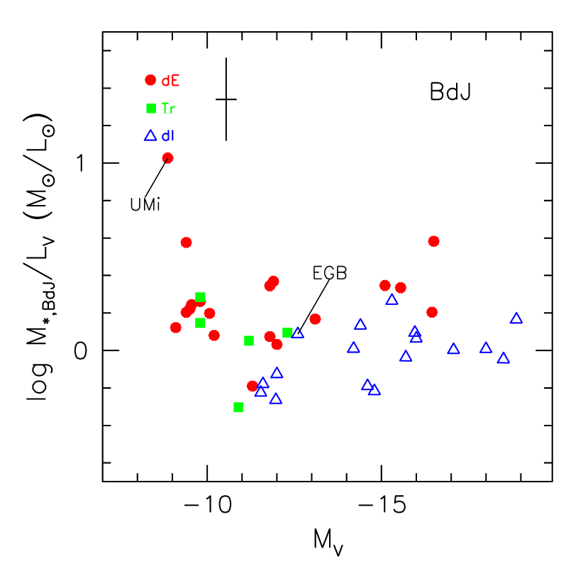
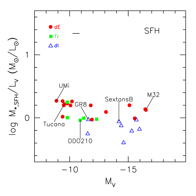
Figure 1: The BdJ and SFH stellar mass-to-light ratios, in the $V$-band, as a function of $M_{V}$.

The $M_{*}/L_{V}$ ratios calculated with the two methods above are plotted against absolute $V$ magnitude in Fig. 1. There is no apparent trend in either plot. The $M_{*}/L$ values calculated through BdJ’s colour-$M_{*}/L$ relation are more scattered than those calculated from inferred SFH’s, likely because BdJ’s colour-$M_{*}/L$ relations were derived for gaseous discs, and are not ideal for early-type dwarf galaxies.

Immediately apparent in both plots is an offset in $M_{*}/L$ between dI and dE galaxies. The dE’s have a higher $M_{*}/L$ on average than dI’s, as expected from their older, redder, stellar populations. Median values for $M_{*}/L$ according to type are given in Table 2.

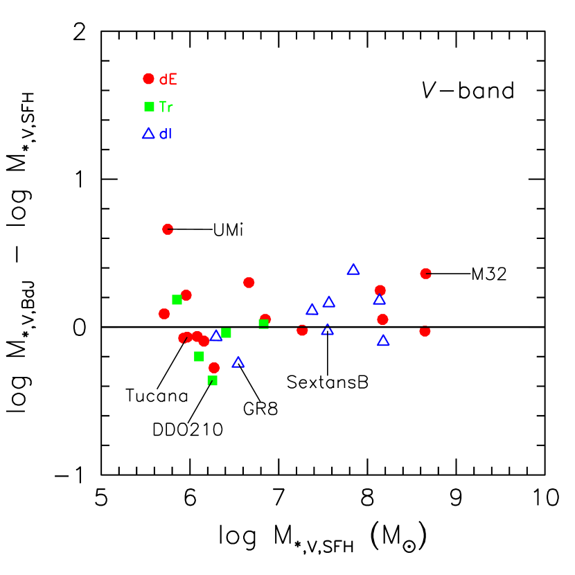
Figure 2: Difference in stellar masses computed via BdJ and SFH.

The abnormally high $M_{*}/L$ ratio for Ursa Minor dSph (UMi) seen in the plot for BdJ values reflects its unusually red colour (see Table 1). UMi’s redness makes it an outlier also in Fig. 2. However, the $M_{*}/L$ estimated from the SFH approach, which does not require colour information, yields a reasonable value in agreement with the observed trend for other Local Group galaxies.

We compare in Fig. 2 the stellar masses computed from the $M_{*}/L$ ratios of the two methods. There is good agreement, with the exception of UMi.

The stellar masses and stellar mass ratios computed through BdJ are generally slightly higher than those computed via SFH. This may be explained by the fact that BdJ calibrated their colour-$M_{*}/L$ correlation under the assumption of maximal discs, making the BdJ $M_{*}/L$ ratios upper limits.

The distribution of stellar masses, $M_{\rm*}$, against absolute $V$ magnitude, $M_{V}$, is shown in Fig. 3. The solid line has a forced slope of -0.4, while the zero-point is adjusted to fit the data. Once again, the $M_{\rm*}$ values for the dI galaxies tend to fall below the dE’s as a result of the younger populations in dI’s.

Both methods of calculating $M_{*}/L$ yield comparable values of log $M_{\rm*}$ within 3% (see Table 2). Thus, the observed luminosity scaling relations (e.g. $\Sigma-L$, [Fe/H]-$L$, $R_{e}$-$L$, [O/H]-$L$, $V$-$L$, $\sigma-L$) will remain intact when translating them to physical scaling relations.

Table 2: Median $M_{*}/L$ for different galaxy types

		$B$-Band			$V$-Band
		SFH	BdJ		SFH	BdJ
dI		0.5	0.6		0.7	0.8
Tr		0.7	0.8		1.0	1.0
dE		1.5	1.1		1.6	1.3

2.1.3 Choice of Methods

Given the incompleteness of our original data bases, we establish various guidelines in Table 3 to assign final $M_{*}/L$ values per galaxy.

We can use a median $M_{*}/L$ value for all the galaxies according to Hubble type, or assign the $M_{*}/L$ for each galaxy based on the BdJ or SFH methods. The first option recognises the uncertainties of both methods of calculating $M_{*}/L$ (namely, the uncertainties in the SFH, and the uncertainties in extrapolating BdJ’s colour-$M_{*}/L$ correlation down to dwarf galaxies), while the second method uses the full available data to make educated guesses for $M_{*}/L$. We have thus created two data sets of stellar data according to these methods, calling the first “a,” and the second “b.”

For the “a” set, we assign the average of the SFR and BdJ median values of the $M_{*}/L$ from Table 2. For the “b” set, we first shift the BdJ $M_{*}/L$ ratios down so that their median values per Hubble type match those from SFH. We then assign their $M_{*}/L$ ratios according to our prescription in Table 3.

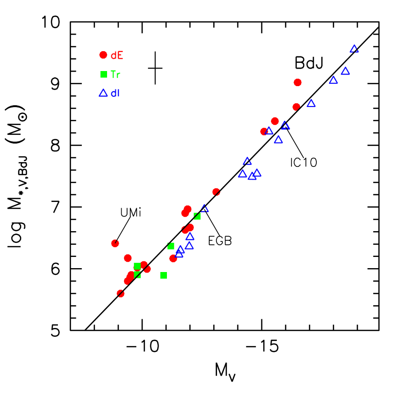
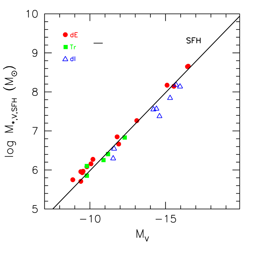
Figure 3: Comparison of stellar masses with the absolute magnitude $M_{V}$. The BdJ and SFH computed values are on the left and right respectively. The solid line has a forced slope of -0.4 and a free vertical offset.

The “a” and “b” sets are consistent with each other within their errors, and our choice of “a” or “b” makes no difference to our conclusions. In the subsequent analysis, we employ the “b” set since it utilises all the available data to calculate $M_{*}/L$, and preserves any intrinsic scatter.

2.2 Surface Density

The luminosity profiles of the dI and dE galaxies have been fitted (M98 and references therein) with an exponential function whose inner extrapolation provides the central surface brightness $\Sigma_{0}$, which we translate to a stellar surface density, $\mu_{*}$ (${\rm M}_{\odot}{\rm kpc}^{-2}$) using the $M_{*}/L$ derived above.

M 32 has a very high central surface brightness of 11.5 mag arcsec^-2 (GGH03), yielding $\log\mu_{*}=12.1$ (${\rm M}_{\odot}~{}{\rm kpc}^{-2}$). This is four orders of magnitude higher than other galaxies of similar luminosity. M 32 indeed belongs to the rare class of compact dwarf galaxies (e.g. Ziegler & Bender, 1998; Mieske et al., 2005, and references therein). We thus exclude M 32 from analyses involving $\mu_{*}$. However, we retain it for other tests.

2.3 Velocity

The velocity data for the dwarf galaxies consist of a rotational velocity (corrected for inclination), $V_{\rm rot}$, and/or a projected central velocity dispersion, $\sigma$. The dI’s typically have a rotation velocity that is larger than the velocity dispersion (exceptions are Leo A, GR 8 and Sag DIG - see Courteau et al., 2007b), whereas dE’s only have a measurable velocity dispersion.

We wish to define as a global parameter a characteristic velocity $V$ that will represent in both cases the depth of the potential well, which for dwarf galaxies is believed to be dominated by the dark halo. The measured rotation velocity in the disky dI’s is taken as is, assuming that it approximates the virial halo velocity and is a near lower bound to the maximum rotation velocity. We then ask, what does a dE’s velocity dispersion tell us about its potential well? What would have been its rotation velocity if it had been disky in the same halo with the same stellar mass? To answer these questions, given the tightness of the Tully-Fisher (TF) relation, we assume that the halo mass scales with the stellar mass in the same way for both dE’s and dI’s (refer to §4.1) and adopt the following algorithm: take $V={\rm max}\{V_{\rm rot},X\sigma\}$ (or the appropriate value when only one of $V_{\rm rot}$ and $\sigma$ is available) where $X$ is chosen to minimise the scatter in the TF relation (log $V$ vs. log $M_{\rm*}$). We find that $X=1.92$ which is consistent with the $V$-$\sigma$ relation for large disc galaxies (Courteau et al., 2007b), but is larger than the $X=\sqrt{2}$ solution for an isothermal sphere. Had we chosen to minimise the baryonic Tully-Fisher (BTF) relation instead, we would have found a lower value of $X$ but slightly larger scatter than for the TF relation for these dwarf galaxies (see also §4.1 for further motivation to minimize the TF instead of the BTF relation). The choice of the isothermal solution $X=\sqrt{2}$ would yield a TF relation that is slightly steeper (in log $V$ vs. log $M_{\rm*}$), but the galaxy types still form a single relation. Furthermore, the results of our PCA analyses (described in §3) are statistically identical for both $X=\sqrt{2}$ and $X=1.92$.

In summary, our algorithm sets $V=X\sigma$ for the dE galaxies, and $V=V_{\rm rot}$ for the dI galaxies (except for GR 8, Leo A and Sag DIG where $\sigma$ is greater than the maximum $V_{\rm rot}$ of the ISM).

2.4 Radius, Baryon Mass, Metallicity and SFR

We use the exponential scale length scaled with the distance estimates provided in M98 as the characteristic stellar radius of galaxies. We also use the H 1 mass provided by GGH03 and our derived stellar mass to estimate a baryonic mass. For most of the dE’s the quoted H 1 mass is an upper limit.

Iron abundances [Fe/H] are taken from GGH03, which are based on spectroscopic and photometric measurements of red giant branch stars. GGH03 use the mean abundances of the old stellar populations which can be consistently measured across the galaxy types. Oxygen abundances are available only for galaxies with current star formation, so besides the dI’s, only four dE’s and one Tr galaxy have available oxygen data. Thus, we use the iron abundances to trace the total metallicty $Z$ and assume a linear relation between them. Recalling that [Fe/H] is logarithmic, we then define $Z$ as:

$$\log(Z/Z_{\odot})={\rm[Fe/H]}$$ (1)

where we adopt $Z_{\odot}=0.019$ (Anders & Grevesse, 1989; Girardi et al., 2000; Carraro et al., 2001).

The current star formation rate (SFR or $\dot{M}_{*}$) data for the dI galaxies, estimated from observed H$\alpha$ flux, are taken directly from M98 or vdB00. dE galaxies have very little or no current star formation.

Table 3: $M_{*}/L$ assignments for data set “b”

	Case 1	Case 2	Case 3
dI	average $M_{*}/L$ ratios from BdJ and SFH	whichever datum exists	$M_{*}/L$ from data set “a”
dE	$M_{*}/L$ from SFH	whichever datum exists	$M_{*}/L$ from data set “a”
Tr	$M_{*}/L$ from SFH

Note. — The cases are: 1. enough data exist to calculate $M_{*}/L$ from both SFH and BdJ methods; 2. data exist for only one method of computing $M_{*}/L$; 3. not enough data exist for either SFH or BdJ methods. (For Tr galaxies, only Case 1 applies.)

2.5 Error bars

Due to the uncertainties in the determination of $M_{*}/L$ and the heterogeneous data base, error bars are not taken into account in the subsequent analysis. However the typical error bar size relative to the scatter in distribution of the galaxies is shown in the upper left corner of all figures. The estimated error bars for $\log M_{\rm*}$ and $\log\mu_{*}$ reflect the difference between the SFH and BdJ calculations $M_{*}/L$, and are on average 4% and 7% of their respective ranges. The error bars are typically 4% for $\log V$ and 10% for $\log Z$ (Eva Grebel, private communication). No estimates are provided for the uncertainty in SFR.

3 Methods of Analysis

Throughout this analysis, we study the relations between the dwarf galaxy structural and SF parameters using linear regression and principal component analysis (PCA).

For the two-dimensional analyses, we investigate the correlation in log space between pairs of the structural and SF quantities. We plot the distribution of each pair, obtain the best-fitting line by the method of bisector least-squares, and calculate the standard Pearson linear correlation coefficient $r$ according to Press et al. (1992).

We use PCA as a tool to quantify the shape of the distribution of the galaxies in parameter space. Given a data set with $m$ parameters (such as stellar mass, metallicity, etc), the PCA quantifies the distribution of the data along orthogonal basis vectors of the parameter space. PCA outputs the vectors V${}_{k},k=1,m$ and their eigenvalues $D_{k}$. Appendix B describes the derivation of V_k and $D_{k}$ (or $D_{k,k}$ as in the Appendix).

The following is an interpretation of the eigenvectors and eigenvalues:

The eigenvectors, which are orthonormal, lie in the directions of greatest variance in the data. The ratios of the eigenvalues are a measure of the relative strength of the variance along each corresponding eigenvector. For example, if the distribution of the data were a line in a parameter space of 3 parameters, the vector V₁ with the largest eigenvalue $D_{1}$ will lie along that line, while the other two vectors will be orthogonal to it. Furthermore, the eigenvalue $D_{1}$ will be much larger than the other two eigenvalues, which will be similar in size, reflecting the extended distribution of the data along V₁, and relatively little extension in the other two directions. Such a distribution is characterised by one primary parameter. If the distribution of the data is a plane in 3-D space, two of the eigenvectors will lie in the plane and will have comparably large eigenvalues, while the third vector, lying orthogonal to the planar distribution will have a relatively small eigenvalue. Such a distribution is characterised by two primary parameters.

In fact, for 3-D space, we can more generally associate a “linear” distribution with “prolate” ($D_{1}$:$D_{2}$ $\gg$ $D_{2}$:$D_{3}$), and a “planar” distribution with “oblate” ($D_{1}$:$D_{2}$ $\ll$ $D_{2}$:$D_{3}$).

In order to meaningfully quantify the shape of the data distribution, we standardise the data before performing the PCA. Standardisation divides the data set by the standard deviation of the parameters, so that the eigenvalues are independent of parameter range. In other words, standardisation gives us a shape for the distribution with the ranges of all the axes on equal footing. Without standardisation the shape of the distribution will change from being linear to planar, depending on their relative scalings. In fact, the scaling relations themselves can be derived directly from the elements of the first eigenvector of the unstandardised analysis. On the other hand, standardisation will output eigenvalues that are independent of the scalings, and therefore insensitive to whether we choose for instance to use $V^{2}$ instead of $V$. Therefore, throughout this study, we present the results of standardised PCA along with the standard deviations of each parameter. (The scaling relations may be recovered by dividing the components of the first principal eigenvector V₁ by the corresponding standard deviations.)

We caution the reader that standardisation assumes a complete, unbiased representation of all galaxy types for all considered parameters. Given the depth of current imaging surveys, we suspect that only much fainter LG dwarfs are truly missing, and our assumption of standardisation is reasonable. Performing our analysis using strictly unstandardised PCA would yield tighter fundamental lines in every case due to the large range of $M_{\rm*}$ relative to the other parameters. Standardisation is nonetheless preferred for the reasons stated above.

In the following sections, we present our 2D and PCA analyses first for the structural parameters, and then for the SF parameters.

4 Results: The Structural Parameters

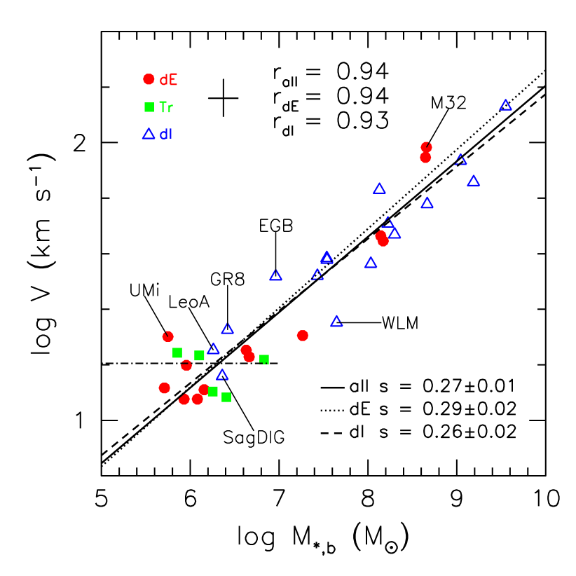
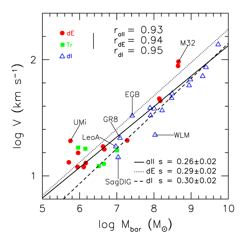
Figure 4: Left: Circular velocity vs. stellar mass for LG dwarf galaxies. Right: Circular velocity vs. “baryonic mass” ($M_{\rm bar}=M_{\rm*}+M_{\rm HI}$). We show bisector fits for all the galaxies (solid), and separately for the dE (dotted) and dI (dashed) types. The dash-dotted line delineates galaxies below $M_{\rm*}=10^{6.9}{\rm M}_{\odot}$. The Pearson correlation coefficient $r$ is shown at the top and the bisector fit slope $s$ at the bottom of each figure.

4.1 2D: Velocity and Mass

Fig. 4 shows the correlation of characteristic velocity versus $M_{\rm*}$ for LG dwarf galaxies with $V\propto M_{\rm*}^{0.27\pm 0.01}$ and $r=0.94$. Recall that $V$ is constructed from $V_{\rm rot}$ and $\sigma$ in such a way as to minimise the scatter in this scaling relation. So naturally, the dI and dE galaxy types seem to lie on the same relation with uniform spread. However, had we used $V=(\sqrt{2}$ or $\sqrt{3})\sigma$ instead of $\sim 2\sigma$ the dI’s and dE’s would still appear to lie on the same relation. Note also that the smallest dwarfs cluster just above $V\sim 10$km s^-1 and could even be described by a constant $V$ (dash-dotted line) which Dekel & Woo (2003) explain might be due to radiative feedback.

The LG dwarf galaxies fall below $V_{c}\lower 2.15277pt\hbox{$\;\buildrel<\over{\sim}\;$}90\,{\rm km}\,{\rm s}^{-1}$. The $V-M_{\rm*}$ relation of LG dI’s is consistent with that of McGaugh (2005), with a slope of $0.26\pm 0.02$ or $M_{\rm*}\propto V^{3.8\pm 0.3}$, which is not significantly different from $M_{\rm*}\propto V^{4}$.

Adding the gaseous mass from GGH03 ($M_{bar}=M_{\rm*}+M_{\rm HI}$) yields a baryonic Tully-Fisher (BTF) slope for the LG dI’s that is significantly shallower ($M_{\rm*}\propto V^{3.3\pm 0.2}$) than that reported by (McGaugh, 2005), but consistent with the BTF relations of both BdJ and Geha et al. (2006) (Fig. 4 left). We also find that for dI’s with log $V$ $>$ 1.5, we find that the scatter in the LG BTF relation is reduced significantly compared to Fig. 4 (right). These dI’s lie almost precisely along the BTF relation found by (McGaugh, 2005), with comparable scatter. McGaugh (2005) describes a break in the distribution of circular velocity versus stellar mass (or total light) for galaxies with $V_{c}\lower 2.15277pt\hbox{$\;\buildrel<\over{\sim}\;$}90\,{\rm km}\,{\rm s}^{-1}$. This break however disappears if $V_{c}$ is plotted against total (luminous + gaseous) mass.

The shallower overall slope of the dI BTF relation is likely due to the different prescriptions for calculating $M_{*}/L$. McGaugh (2005) used an optimal empirical relation (see their section 3.3), while we used stellar population models, as did BdJ (see §2.1). McGaugh (2005) showed that this difference in methods is enough to account for the shallower BTF slope found by BdJ (which is consistent with ours).

The contribution of the H 1 mass to dE galaxies is negligible and we find two distinctly offset BTF relations for dI and dE galaxies. (This is true even had we used $V=\sqrt{2}\sigma$ for the dE’s.) This offset would have been larger had we used the suggestion of Pfenniger & Revaz (2005) that $M_{bar}=M_{\rm*}+3M_{\rm HI}$. This suggests that although the BTF may more fundamentally describe the kinematics of dI’s, the stellar relation (i.e. the TF) may be a more fundamental description of the entire dwarf population (since the same TF describes all galaxy types). (Recall also that had we minimised the scatter of the BTF in determining the $X$ of §2.3, the scatter of the BTF would have been slightly larger than the minimised scatter of the TF.) Using baryon mass instead of stellar mass also increases the offset between the types in the $R_{*}-M_{\rm bar}$, $\mu_{*}-M_{\rm bar}$, and $Z-M_{\rm bar}$ relations.

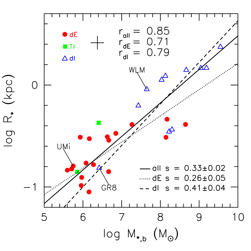
Figure 5: Exponential radius vs. stellar mass. We plot the two-dimensional linear regression on all the galaxies (solid), and separate fits to the dE (dotted) and dI (dashed) types.

4.2 2D: Radius and Mass

Fig. 5 shows the correlation between exponential radius and stellar mass fitted as $R_{*}\propto M_{\rm*}^{0.33\pm 0.02}$, with $r=0.85$. The galaxy types populate different regimes of the relation, with dI galaxies being bigger and more massive than dE’s, yet they are both described by the same $R_{*}-M_{\rm*}$ relation. This is interesting in itself as it may indicate a similar physical origin to the relation, (such as halo mass), which may simultaneously be responsible for their differences.

Shen et al. (2003) have plotted the median of the distribution of the sizes of the SDSS galaxies as a function of stellar mass (see their Fig. 11). The sizes are measured for the $z$-band and are given as Sersic half-light radii. If we neglect bandpass differences, we can make a rough comparison of the LG data with SDSS data. Considering that the exponential half-light radius is $R_{1/2}=1.68R_{*}$, we find that the LG dE’s appear to be the low-mass extensions of the early-type distributions of sizes for the SDSS galaxies. The SDSS early-type galaxies follow the relation $R_{*}\propto M_{\rm*}^{0.55}$ while LG dE’s have a shallower $R_{*}\propto M_{\rm*}^{0.26\pm 0.05}$. This shallower slope is consistent with the lower end of the size-luminosity relation of Graham & Worley (2008) while we extend their relation to lower masses.

However, while the LG dI’s overlap the $R_{*}-M_{\rm*}$ relation of the SDSS late-type galaxies, they extend the relation which a steeper slope of $0.41\pm 0.04$ compared to the slope of $0.15$ at the low-mass end of the SDSS sample.

We can derive a stellar size-mass, $R_{*}-M_{\rm*}$, relation for large spiral galaxies from the compilation of scaling parameters for 1300 local disc galaxies by Courteau et al. (2007a). We use the $I$-band exponential scale radii and luminosities, $V-I$ colours, and colour-$M_{*}/L$ relations of BdJ (see Dutton et al., 2007) to derive a $R_{*}-M_{\rm*}$ relation for large galaxies. We find that the dI’s overlap with the $R_{*}-M_{\rm*}$ relation of bigger disk galaxies and with comparable slope.

4.3 2D: Surface Mass Density and Mass

The dependence of radius and stellar mass is also expressed via the relation for stellar surface density ($\mu_{*}\propto M_{\rm*}/R_{*}^{2}$) and stellar mass. Fig. 6 shows a correlation between $\mu_{*}$ and $M_{\rm*}$ that spans 4.5 decades in $M_{\rm*}$ and 3 decades in $\mu_{*}$. The best-fitting relation is $\mu_{*}\propto M_{\rm*}^{0.61\pm 0.05}$ with $r=0.81$.

With the exception of WLM and GR 8, dI galaxies have a lower mean surface mass density than dE’s. Since both $M_{\rm*}$ and $\mu_{*}$ depend on $M_{*}/L$ in the same way, plotting $\mu_{*}$ against $M_{\rm*}$ or $L$, as previously done by GGH03, yields identical offsets between the dE and dI types. These best fit lines have the same slope of $0.74\pm 0.05$, but are offset by about 0.5 dex from the centre of the distribution.

Kauffmann et al. (2003b, see their Fig. 7) showed an analogous distribution in the plane of surface density (within the half-light radius) versus stellar mass for 123,000 SDSS galaxies with $M_{\rm*}>10^{8}{\rm M}_{\odot}$. They find a weak systematic dependence of about $\mu_{*}\propto M_{\rm*}^{0.2}$ (our eye-ball estimate) for the HSBs and $\mu_{*}\propto M_{\rm*}^{0.63}$ (their quote) in the LSB regime with $10^{8}<M_{\rm*}<3\times 10^{10}{\rm M}_{\odot}$. After considering the $\mu_{*}-\mu_{e}$ conversion, the LG dwarf galaxies extend this relation down to $8\times 10^{5}{\rm M}_{\odot}$ and together, their $\mu_{*}-M_{\rm*}$ relation is consistent with $\mu_{*}\propto M_{\rm*}^{0.6}$.

Shen et al. (2003) showed the median of the same distribution, but separated into late and early-type distributions. They show that the early-types tend to have higher surface density, consistent with our finding for LG galaxies. In fact, the LG dE’s and dI’s again seem to extend early and late-type surface density relations to lower masses. (Our eye-ball estimate of their slopes: $\sim 0.65$ for both late- and early-types, compared to $s=0.61\pm 0.05$ for LG dwarfs).

Vaduvescu et al. (2005) studied a sample of 34 dI galaxies and provided central surface brightnesses and $K$ and $J$-band magnitudes for these galaxies using a hyperbolic secant (sech) function to fit their surface brightness profiles. Using the colour-$M_{*}/L$ relations of Bell & de Jong (2001), we converted their sech magnitudes and central surface brightnesses to stellar quantities, and compared their $M_{\rm*}$-$\mu_{*}$ relation to that of the LG dwarf galaxies. We find that the $M_{\rm*}$-$\mu_{*}$ relation is significantly tighter ($r=0.86$) than their magnitude relation ($M_{K,{\rm sech}}$-$\mu_{0,{\rm sech}}$, $r=0.71$). Secondly, we find that their dI’s lie neatly along the same $M_{\rm*}$-$\mu_{*}$ relation as the LG dwarf galaxies, even though the surface brightness profiles of the LG dwarfs were fit to exponential functions. We plot the data from Vaduvescu et al. (2005), which we converted to stellar quantities, together with the LG data in Fig. 7.

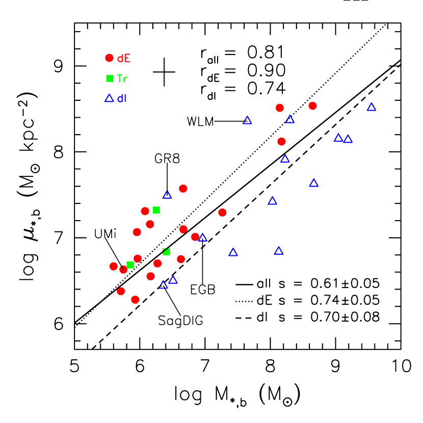
Figure 6: Central stellar surface density vs. stellar mass. We plot the two-dimensional linear regression line of all the dwarf galaxies (solid), and separate regressions for the dE (dotted) and dI (dashed) types.

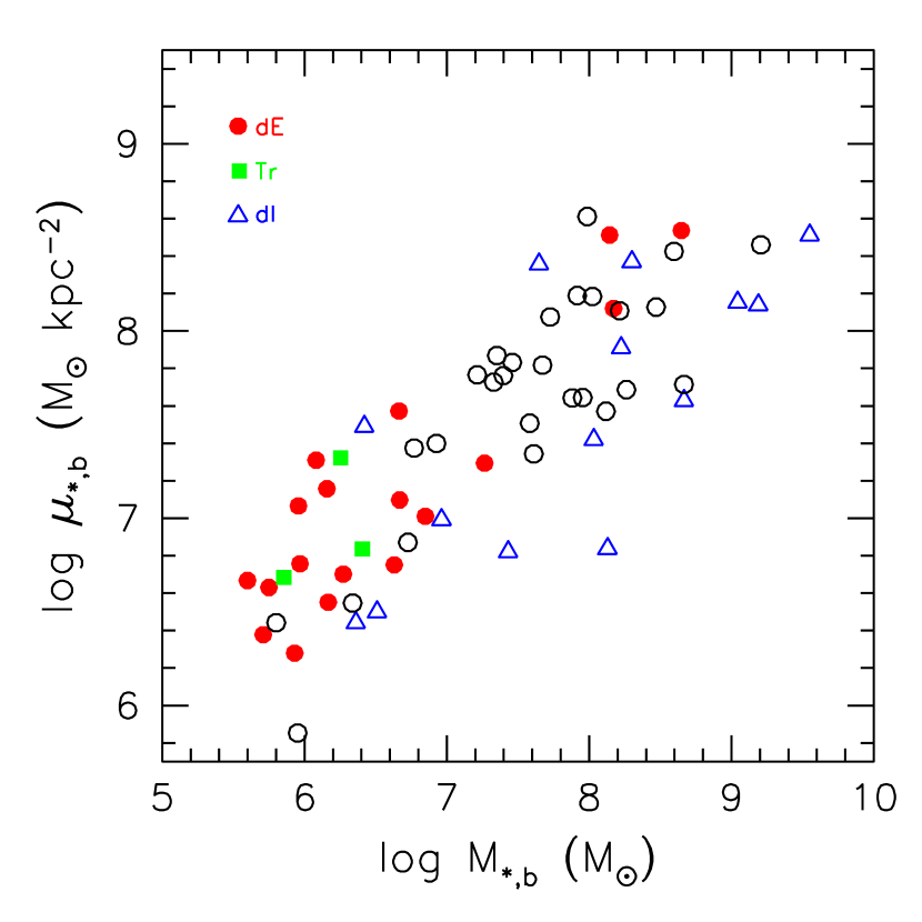
Figure 7: The $M_{\rm*}$-$\mu_{*}$ relation of the LG dwarf galaxies plotted together with the dI’s of Vaduvescu et al. (2005) (open circles).

4.4 PCA: The Fundamental Line in Structural Space

We use PCA as outlined in §3 to quantify the shape of the distribution of the LG dwarf galaxies in the (log) space of the structural parameters ($M_{\rm*}$, $R_{*}$, $V$). We present the results graphically in Fig. 8 and quantitatively in Table 4.

Fig. 8 shows the axes Y_j (defined in Appendix B) as the coordinates of the data vectors projected onto V_j, for $j=1...3$. Each panel represents different views along the three dimensions of the distribution. On visual inspection, the shape of the distribution is linear in Fig. 8.

We list the components of the three V_j vectors in Table 4. The first vector points in the direction of the fundamental line in this scaled basis. The other two vectors point in the directions orthogonal to the line. By construction, the components of the first principal vector V₁ are $\sim 1/\sqrt{n}$ where $n$ is the number of dimensions (in this case 3) since standardisation places all the data along a diagonal. The vector components are in the basis of the original four parameters scaled by their standard deviations, from which the scaling relations are derived. (In the unstandardised analysis, the scaling relations are recovered directly from the components of the first eigenvector.) For example, if the first eigenvector is V₁, and its $j$’th component is V₁($j$), then the scaling relation between the parameters log $M_{\rm*}$ and log $V$ is

$$\frac{{\bf V}_{1}(M_{\rm*})/\sigma_{M_{\rm*}}}{{\bf V}_{1}(V)/\sigma_{V}}=\frac{0.60/1.22}{0.58/0.32}$$ (2)

yielding $\log V\propto(0.27\pm 0.01)\log M_{\rm*}$ which is consistent with the 2-D fit in §4.1. The scaling relation between log $M_{\rm*}$ and log $R_{*}$ is listed in the note under Table 4, and is also consistent with the 2-D fit in §4.2.

The eigenvalues associated with the principal vectors quantify the shape of the distribution of the data. The eigenvalue associated with the first principal vector is $90.1\%$ of the sum of all the eigenvalues. The strength of the second eigenvalue is only $8.4\%$. The variance along the first principal vector is more than $10$ times greater than the variance along the second principal vector. The ratio of the second-to-third eigenvalues is only $5.6$. In other words, the extensions of the data along the second and third principal vectors are more similar to each other than they are to the extension of the data along the first principal vector. This describes a linear or prolate distribution, according to the criteria in §3, and is characterised by one primary parameter.

The standard method of displaying fundamental lines or planes (edge-on) from PCA is to plot one parameter against a linear combination of the other parameters. So the LG data would be plotted as $\log M_{\rm*}$ versus

$$(2.92\pm 0.31)\log V+(0.72\pm 0.32)\log R_{*}+(3.35\pm 0.23)$$ (3)

from the third principal vector. This is equivalent to displaying only the upper-left panel in Fig. 8, but rotated so that the log $M_{\rm*}$ lies along the $y$-axis, and scaled so that the data lie on the $y=x$ line. Such a presentation of the data, with its confusing mix of parameters on its $x$-axis, is not spatially intuitive as it fails to display their distribution from other angles. We feel that our method of displaying the output of PCA is more useful since the data are displayed along all the principal axes of their distribution, giving the viewer a more intuitive feel for its shape.

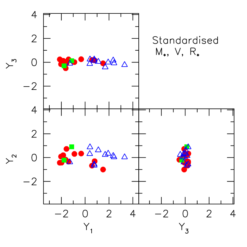
Figure 8: The fundamental line in structural space. The axes lie in the directions of the V_j eigenvectors defined in the text and the data are projected onto them. The components of the eigenvectors are given in Table 4.

Table 4: PCA results in structural space

$X$	$\log M_{\rm*}$	$\log V$	$\log R_{*}$	Eigen-	Ratios
				values (%)
V1	0.60 $\pm$ 0.01	0.58 $\pm$ 0.01	0.56 $\pm$ 0.01	90.1 $\pm$ 3.2	}10.7$\pm$ 3.9
V2	-0.23 $\pm$ 0.08	-0.54 $\pm$ 0.07	0.81 $\pm$ 0.03	8.4 $\pm$ 3.0	}5.6$\pm$ 2.7
V3	0.77 $\pm$ 0.02	-0.61 $\pm$ 0.06	-0.19 $\pm$ 0.08	1.5 $\pm$ 0.5
$\sigma_{X}$	1.22	0.32	0.41

Note. — The scaling relations from the principal vector:
$\log V$ $\propto$ (0.27 $\pm$ 0.01)$\log M_{\rm*}$, $\log R_{*}$ $\propto$ (0.36 $\pm$ 0.01)$\log M_{\rm*}$.
Standard projection:
$\log M_{\rm*}$=(2.92 $\pm$ 0.31)$\log V$+(0.72 $\pm$ 0.32)$\log R_{*}$+(3.35 $\pm$ 0.23).

We also performed PCA on an “alternate” structural parameter space where we have replaced $R_{*}$ with $\mu_{*}$ in the above structural space. We summarise the results in Fig. 9 and Table 5. The distribution of the galaxies is triaxial in this space since the ratios of the eigenvalues (listed in the table) are comparable. However, since the first eigenvalue is at least ($8.0$) times greater than the other eigenvalues, meaning that the galaxies are at least $8$ times more extended along one axis than the along the other axes, we say that the galaxies lie in a linear distribution, characterised by one primary parameter, in this alternate structural space.

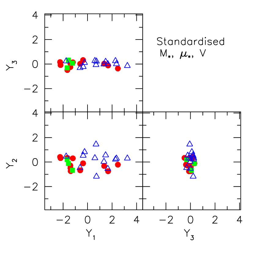
Figure 9: Projections of the LG dwarf data in an alternate structural space. The components of the PCA eigenvectors are given in Table 5.

Table 5: PCA results in alternate structural space

$X$	$\log M_{\rm*}$	$\log\mu_{*}$	$\log V$	Eigen-	Ratios
				values (%)
V1	0.60 $\pm$ 0.01	0.54 $\pm$ 0.02	0.58 $\pm$ 0.01	87.5 $\pm$ 3.8	}8.0$\pm$ 2.7
V2	0.24 $\pm$ 0.06	-0.82 $\pm$ 0.02	0.51 $\pm$ 0.05	11.0 $\pm$ 3.7	}7.0$\pm$ 3.2
V3	0.76 $\pm$ 0.02	-0.17 $\pm$ 0.07	-0.63 $\pm$ 0.04	1.6 $\pm$ 0.5
$\sigma_{X}$	1.19	0.71	0.32

Note. — The scaling relations from the principal vector:
$\log\mu_{*}$ $\propto$ (0.66 $\pm$ 0.03)$\log M_{\rm*}$, $\log V$ $\propto$ (0.27 $\pm$ 0.01)$\log M_{\rm*}$.
Standard projection:
$\log M_{\rm*}$=(0.35 $\pm$ 0.15)$\log\mu_{*}$+(3.00 $\pm$ 0.24)$\log V$+(0.28 $\pm$ 0.37).

5 Results: The Star Formation (SF) Parameters

5.1 2D: Metallicity and Mass

Fig. 10 shows metallicity versus $M_{\rm*}$. The best-fitting global scaling relation is $Z\propto M_{\rm*}^{0.40\pm 0.04}$ with $r=0.76$. The higher metallicity of dE galaxies relative to the dI galaxies of the same luminosity has been known for some time (see for example M98), and this offset persists even for old stellar populations (GGH03). Not surprisingly, we see the same phenomenon when using $M_{\rm*}$ instead of luminosity. Their respective correlations are much stronger when fitted separately (dE’s: $0.93$; dI’s: $0.88$).

For SDSS data, Kauffmann et al. (2003b) reported $Z\propto M_{\rm*}^{0.4-0.5}$ (depending on the metallicity tracer) for $M_{\rm*}<3\times 10^{10}{\rm M}_{\odot}$, at the bright end of the dwarf galaxy regime (Kauffmann et al., 2003b). This is consistent with our global and type-dependent slopes.

Tremonti et al. (2004) showed more specifically that SDSS star-forming galaxies follow the relation 12 + log [O/H] $\simeq$ 0.35 log $M_{\rm*}$ for $M_{\rm*}<3\times 10^{10}{\rm M}_{\odot}$, with an overall saturation beyond this transition mass (see their Fig. 6). This translates to $Z\propto M_{\rm*}^{0.35}$ at the low-mass end assuming that the oxygen abundances trace $Z$ linearly. Using oxygen abundance data from M98, we find that the LG galaxies follow 12 + log [O/H] $\simeq 0.39\pm 0.04$ log $M_{\rm*}$, consistent with the slope of low mass SDSS galaxies (Fig. 11). Our slope is also a slightly better match to the low-mass end of the SDSS galaxies than that of Lee et al. (2006).

However we find that the LG dwarf galaxies have oxygen abundances that are on average 0.3 dex lower than those of low-mass SDSS galaxies. While oxygen abundances of the LG dwarf galaxies are measured via spectroscopy of H 2 regions (M98), abundances for SDSS galaxies were estimated using empirically and theoretically calibrated relations between metallicity and strong optical emission line flux. Tremonti et al. (2004) notes that aperture bias can lead to overestimates in abundances by about 0.1 dex. They also cite evidence from Kennicutt et al. (2003) that “strong line” methods such as theirs may overestimate the true abundance by as much as a factor of 2. Taking these overestimates into account, the LG dwarf galaxies coincide with the lower end of the SDSS distribution and extend the mass range down by about two magnitudes.

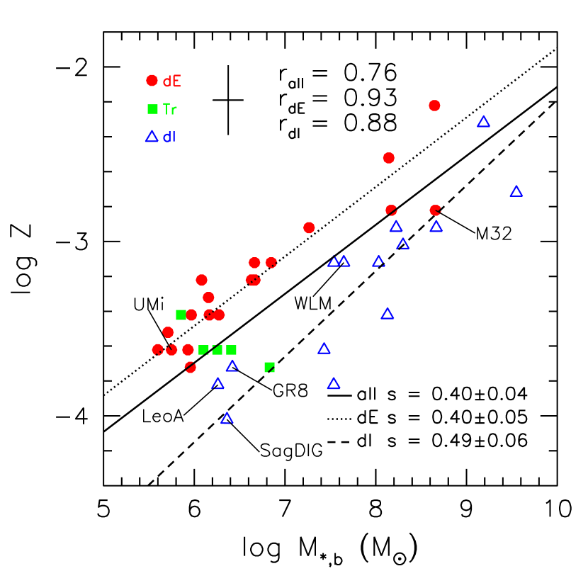
Figure 10: Metallicity vs. stellar mass. We plot the two-dimensional linear regression over all the dwarf galaxies (solid), and separate fits for dE (dotted), and dI (dashed) galaxies.

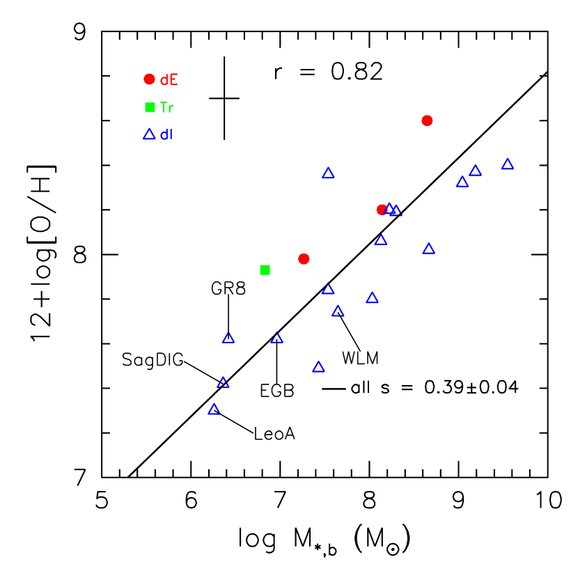
Figure 11: Oxygen abundances of the LG dwarf galaxies vs. stellar mass.

5.2 Star Formation Rate and Mass

Fig. 12 shows the SFR versus $M_{\rm*}$ for dI’s only (and two Tr’s; dE’s have very little or no star formation). The best-fitting scaling relation is $\dot{M}_{*}\propto M_{\rm*}^{1.18\pm 0.08}$ with $r=0.96$.

Brinchmann et al. (2004) (see their figure 17) showed that the low-mass SDSS galaxies follow a SFR-stellar mass relation with a log slope of $\sim$0.7, noticeably shallower than the LG dwarf galaxies. Moreover, the LG dwarf galaxies fall significantly below (almost one order of magnitude at least) the SDSS distribution. Adjusting for the IMF differences in the SFR determinations of M98 (Salpeter IMF) and Brinchmann et al. (2004) (Kroupa IMF) would only increase the vertical offset between them. Since dwarf galaxies have very low metallicities, which normally means very low dust content, the effects of dust extinction would also be stronger at higher mass. Correcting for this would further steepen the LG relation. Underestimation of the Balmer absorption in the H$\alpha$ maps which are used to estimate SFR is also more likely at higher mass (Brinchmann 2005, private communication), and correcting for this would also lead to a steepening of the relation. The different slope and vertical offset between the SDSS and LG galaxies seems to be real, and present a new theoretical challenge. We discuss this further in §6.3.

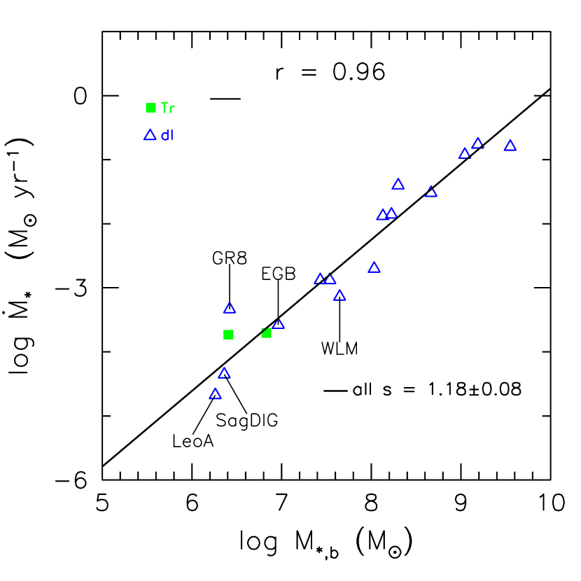
Figure 12: Star formation rate vs. stellar mass. Shown is the two-dimensional linear regression with its slope $s$ indicated as well as the correlation coefficient $r$.

5.3 PCA: The Fundamental Line of the Structural + SF parameters

The above linear correlations motivate an investigation of the fundamental line in higher dimensional spaces than the structural spaces that we have already analysed. Thus, adding the metallicity to the structural spaces, we performed PCA on the 4-D (log) space of $M_{\rm*},R_{*},V,Z$ and on $M_{\rm*},\mu_{*},V,Z$ space, and find that the fundamental line remains linear in these spaces in that the first eigenvalue is much larger than the other three. The line is is illustrated in Fig. 13 and the eigenvalues are listed in Tables 6 and 7.

However, a glance at Fig. 13 reminds us that the dE’s and dI’s are offset in metallicity and suggests that they separately lie in linear distributions. Thus we also perform PCA on the dE’s and dI’s separately.

For the dE’s, we find that their fundamental line lies in the same space as the fundamental line of the whole group but the dE fundamental line is much tighter as indicated by their eigenvalues (listed in Tables 6 and 7), especially in $M_{\rm*},\mu_{*},V,Z$ space (displayed in Fig. 14).

From looking at the ratios of the eigenvalues, the dI’s appear oblate in $M_{\rm*},R_{*},V,Z$ space, and ”quadraxial” in $M_{\rm*},\mu_{*},V,Z$ space. However noting that the first eigenvalue is much larger than the others in both these spaces, the distribution of the data extends mostly in one direction, and is to first order linear. Hence this distribution is also characterised by one primary parameter. Recalling the tight correlation between $M_{\rm*}$ and $\dot{M}_{*}$ in §5.2 for dI’s, we add $\dot{M}_{*}$ to the parameter space and perform the PCA. We find that the dI’s are linearly distributed in this parameter space (see Fig. 16), as indicated by their eigenvalues in Table 8.

Thus we find that, when the stellar evolution parameters $Z$ and $\dot{M}_{*}$ are considered together with the structural parameters, the distribution of all the LG dwarf galaxies remains linear. In particular, the dE’s and dI’s separately form tighter linear distributions in the parameter space of $M_{\rm*},\mu_{*},V,Z$, and also of $M_{\rm*},\mu_{*},V,Z,\dot{M}_{*}$ for the dI’s.

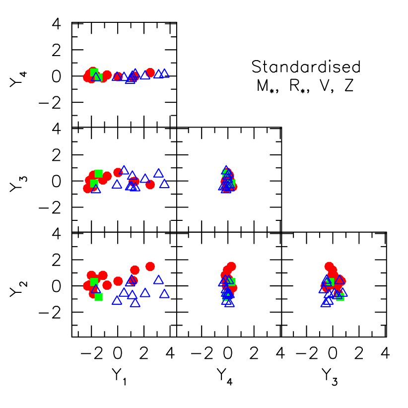
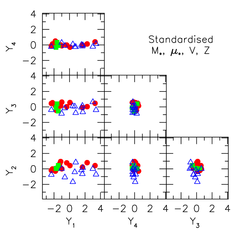
Figure 13: The fundamental line in structural space + metallicity ($M_{\rm*},\mu_{*},V,Z$). The eigenvalues of the PCA are given in Table 7.

Table 6: Eigenvalues for PCA in the parameter space of $M_{\rm*}$, $R$, $V$, $Z$

All galaxies		dE’s only		dI’s only
Values (%)	Ratios	Values (%)	Ratios	Values (%)	Ratios
81.4 $\pm$ 3.9	} 6.2$\pm$ 1.6	84.8 $\pm$ 6.4	} 7.6$\pm$ 3.2	80.9 $\pm$ 8.9	} 7.3$\pm$ 4.0
13.2 $\pm$ 3.4	} 2.8$\pm$ 1.1	11.1 $\pm$ 4.5	} 3.3$\pm$ 2.9	11.1 $\pm$ 6.0	} 1.4$\pm$ 1.0
4.6 $\pm$ 1.2	} 6.4$\pm$ 2.5	3.4 $\pm$ 2.7	} 4.7$\pm$ 4.4	7.7 $\pm$ 3.7	} 23.4$\pm$15.8
0.7 $\pm$ 0.2		0.7 $\pm$ 0.4		0.3 $\pm$ 0.2

Table 7: Eigenvalues for PCA in the parameter space of $M_{\rm*}$, $\mu_{*}$, $V$, $Z$

All galaxies		dE’s only		dI’s only
Values (%)	Ratios	Values (%)	Ratios	Values (%)	Ratios
84.3 $\pm$ 3.9	} 8.6$\pm$ 2.9	92.4 $\pm$ 6.2	} 22.4$\pm$23.3	81.9 $\pm$ 8.1	} 5.7$\pm$ 3.1
9.8 $\pm$ 3.3	} 2.1$\pm$ 0.9	4.1 $\pm$ 4.3	} 1.6$\pm$ 2.0	14.4 $\pm$ 7.7	} 4.5$\pm$ 3.2
4.7 $\pm$ 1.2	} 3.8$\pm$ 1.5	2.6 $\pm$ 1.9	} 3.0$\pm$ 2.6	3.2 $\pm$ 1.4	} 6.4$\pm$ 4.0
1.2 $\pm$ 0.4		0.9 $\pm$ 0.4		0.5 $\pm$ 0.2

Table 8: Eigenvalues for PCA on in the parameter space of $M_{\rm*}$, $\mu_{*}$, $V$, $Z$, $\dot{M}_{*}$

dI’s only
Values (%)	Ratios
83.9 $\pm$ 7.2	} 6.9$\pm$ 3.7
12.2 $\pm$ 6.6	} 4.7$\pm$ 3.4
2.6 $\pm$ 1.3	} 2.5$\pm$ 1.6
1.1 $\pm$ 0.5	} 4.1$\pm$ 2.5
0.3 $\pm$ 0.1

6 DISCUSSION

We have studied the scaling relations of the dwarf galaxies in physical quantities and quantified the “fundamental line” (FL) in the parameter space of these quantities. The following summarises how we achieved those goals and our results.

6.1 The Data

To derive the physical stellar mass, we used a combination of two methods to derive stellar mass-to-light ratios. These methods involved the colour-$M_{*}/L$ relations of Bell & de Jong (2001) (updated by Bell et al., 2003), and SF histories of LG galaxies coupled to population models of BC03.

We divided the six parameters ($M_{\rm*}$, $R_{*}$, $\mu_{*}$, $V$, $Z$, $\dot{M}_{*}$) into two categories. The first category is the “structural” quantities ($M_{\rm*}$, $\mu_{*}$, $R_{*}$, $V$), and the second is the “star formation” (SF) quantities ($Z$, $\dot{M}_{*}$). We treat the stellar mass as the independent parameter and determine the scaling relations of the other quantities with respect to it. We list these scalings in Table 9. Although we have used only the bisector fits, for comparison with other studies, we include in this table the slopes for the 1-D forward least squares fits.

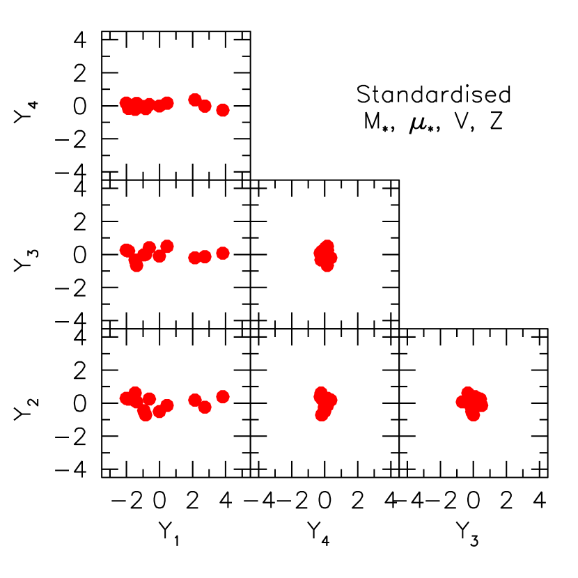
Figure 14: Projections of the dE data in structural space + metallicity ($M_{\rm*},\mu_{*},V,Z$). The eigenvalues of the PCA are given in Table 7.

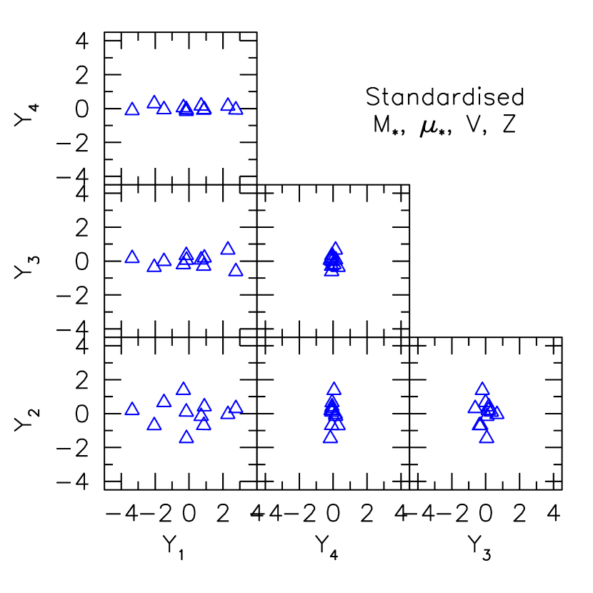
Figure 15: Projections of the dI data in structural space + metallicity ($M_{\rm*},\mu_{*},V,Z$). The eigenvalues of the PCA are given in Table 7.

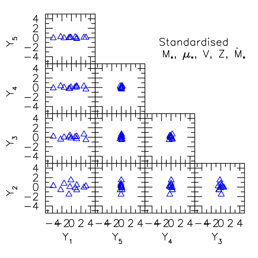
Figure 16: Projections of the LG dI’s in parameter (log) space of $M_{\rm*}$, $\mu_{*}$, $V$, $Z$ and $\dot{M}_{*}$. The components of the PCA eigenvectors are given in Table 8.

6.2 The Structural Scaling Relations

We find that the scaling relations for LG dwarf galaxies extend the corresponding relations found in larger galaxies. Among the structural scaling relations, the $M_{\rm*}$-$\mu_{*}$ relation of the LG dwarfs match that of the lower-mass regime in the SDSS, and extend the range of the relation to about $10^{6}{\rm M}_{\odot}$. This relation is also consistent with that found by Vaduvescu et al. (2005) after converting their photometric data to stellar quantities. The $M_{\rm*}$-$R_{*}$ for the LG dI galaxies also seem to extend the corresponding relation for large disc galaxies (Courteau et al., 2007a), and that of the late-type galaxies in the SDSS (Shen et al., 2003) but with steeper slope.

The slope of the TF relation for the LG dwarf galaxies is consistent with that found by McGaugh (2005) though we do not find their reported break at 90 $\,{\rm km}\,{\rm s}^{-1}$. The LG dwarf galaxies follow a smooth TF relation with no indication of a mass or velocity scale. When adding the H 1 mass, the LG dI’s follow a BTF relation that matches that of McGaugh (2005) above $V=32\,{\rm km}\,{\rm s}^{-1}$, with reduced scatter. However, including all the dI’s yields a shallower slope compared to the optimal slope of McGaugh (2005), but consistent with BdJ and Geha et al. (2006). McGaugh (2005) contended that the BTF slope is sensitive to the method used to determine $M_{*}/L$, so our shallower slope is expected.

6.3 The SF Scaling Relations

The $M_{\rm*}$-$Z$ relation also appears to be a low-mass extension of the relation for the SDSS galaxies.

The slope of the $\dot{M}_{*}$-$M_{\rm*}$ relation for the LG dI’s ($1.18\pm 0.08$) is significantly steeper than that of the SDSS star-forming galaxies (0.7, Brinchmann et al., 2004). Additionally, the LG dI’s fall at least one order of magnitude below the SDSS distribution. Correcting for IMF differences and observational effects such as dust and Balmer absorption worsens this discrepancy. This real vertical offset and steeper slope suggests some environmental effect on current star formation.

Using the SFR data from Skillman et al. (2003) for the Sculptor Group dwarf galaxies, and a $M_{*}/L_{B}$ value of 0.6 (the average of the $B$-band SFR and BdJ values from Table 2 for dI’s) to estimate their stellar masses, we find that the Sculptor Group dwarfs lie along the same $M_{\rm*}$-SFR relation as LG dwarfs. In addition, using the H$\alpha$ data from Gavazzi et al. (1998) for the Coma cluster dwarf galaxies, the Kennicutt (1998) relation between H$\alpha$ and SFR , and the same $M_{*}/L_{B}$ value to estimate their $M_{\rm*}$, we find that the Coma cluster dwarf galaxies roughly lie on the SFR-$M_{\rm*}$ relation of the SDSS (see Fig. 17). Since we expect that the average SDSS galaxy lies in denser environments than the Local and Sculptor Groups, these observations suggest that the SFR-$M_{\rm*}$ relation for dwarf galaxies depends on environment.

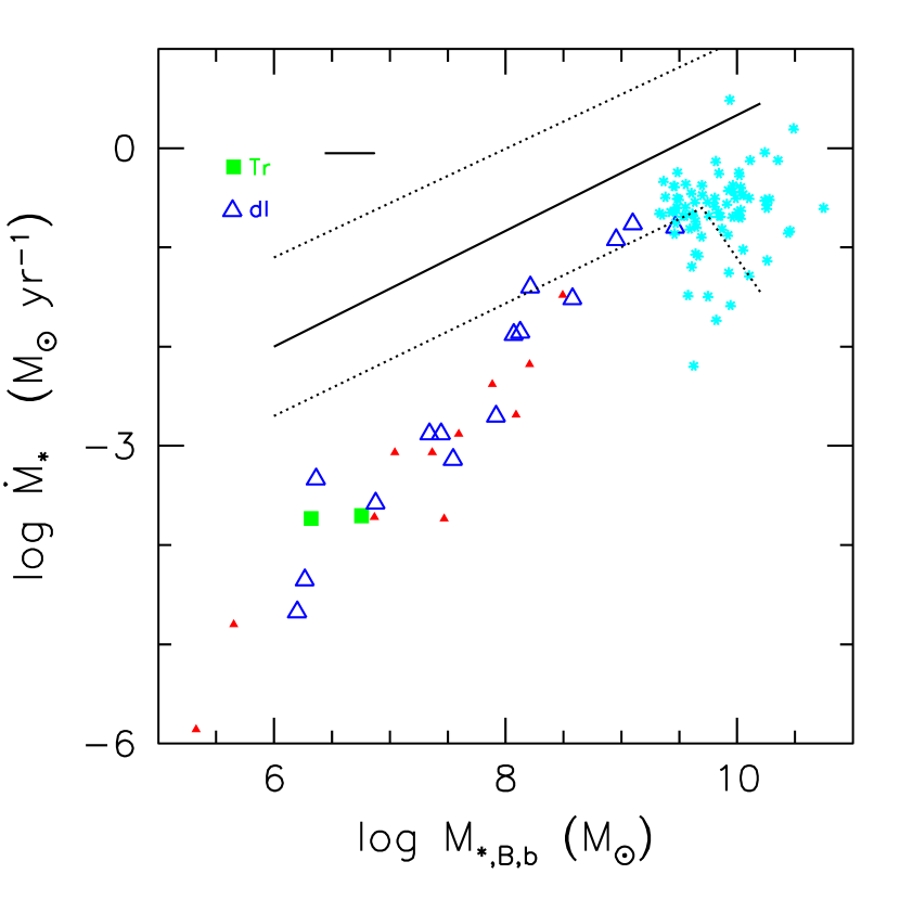
Figure 17: SFR data for the Sculptor Group dwarf galaxies (solid red triangles) and the Coma Cluster dwarf galaxies (cyan stars) plotted together with the LG dI and Tr galaxies (blue and green). Data for the Sculptor Group is taken from Skillman et al. (2003), and for the Coma Cluster, we used Gavazzi et al. (1998). We assume a $M_{*}/L_{B}$ value of 0.6, and adopt the prescription of Kennicutt (1998) to estimate SFR from H$\alpha$ measurements. The solid line is roughly (estimated by eye) the mode line of the distribution of SFR in bins of log $M_{\rm*}$ for the SDSS, while the dotted lines roughly mark the lines where the conditional likelihood of SFR a given $M_{\rm*}$ is equal to 0.02 (see Fig. 17 of Brinchmann et al., 2004).

6.4 The “Fundamental Line” of the LG Dwarf Galaxies

We have used PCA to quantify the distribution of the LG dwarf galaxies in the parameter (log) space of the structural quantities alone, and also of the structural + SF quantities. We make use of the output of PCA to display the full dimensionality and extent of the distribution of the galaxies from the most useful orthogonal angles.

Using PCA, we find that the LG dwarf galaxies (all types) form one linear distribution in structural space $M_{\rm*},\mu_{*}$ (or $R_{*}$), $V$. Despite the fact that dE’s tend to have higher $Z$ than dI’s, the distribution of the entire dwarf population remains linear when we add $Z$ to the parameter space. Since this fundamental line resides in the same space with consistent slopes as those predicted by supernova feedback models ($M_{\rm*},\mu_{*}$ (or $R_{*}$), $V,Z$ space), we call this space “SNF” space (Dekel & Woo, 2003).

Since the star formation properties of dE’s and dI’s differ appreciably, especially $Z$, we performed PCA on dE’s and dI’s separately. We find that the dE’s form an even tighter linear distribution in SNF space. The dI’s are also linear in SNF space, and are even tighter in the space spanned by $M_{\rm*},\mu_{*},V,Z,\dot{M}_{*}$.

The linearity of these distributions suggest that one primary parameter governs their physics. Furthermore because dI’s tend to be more massive than the dE’s, halo mass may be one of the drivers of the distinction between the two types.

Comparison with Previous Work

PB02 found a “fundamental line” in the parameter space (to which we will refer as “PB”) of total mass-to-light ratio $M_{\rm tot}/L_{V}$, metallicity [Fe/H], and central surface brightness $\Sigma_{V}$ (see also Simon et al., 2006). For $M_{\rm tot}/L_{V}$, PB02 used total masses, estimated dynamically, and total luminosity. PB space can be derived from SNF space through the following relations:

$$M_{\rm tot}/L_{V} = V^{2}R/L\propto V^{2}R/M_{\rm*}\propto V^{2}/\sqrt{M_{\rm*}\mu_{*}}$$

$$\Sigma_{V} \propto -2.5\log\mu_{*}$$

$${\rm[Fe/H]} \propto \log Z.$$ (4)

PB space is simply SNF space collapsed into three dimensions. We have improved on their analysis in two ways. Firstly, we included more dI’s in our sample which contribute enough scatter so that it is no longer linear in PB space. Secondly, we have broken PB space into three independent structural parameters ($M$, $V$, and $R$), and metallicity $Z$. PB space relates the three structural parameters by only one relation, namely $\log M_{\rm tot}/L_{V}\propto 0.67\log\mu_{*}$ (PB02), which translates to one projection of the distribution. A linear distribution in the three-space of the structural parameters should be described by two orthogonal projections which we graphically and quantitatively present.

Table 9: Scaling Relations

vs. $\log M_{\rm*}$	$s_{\rm bis}$	$b_{\rm bis}$	$\sigma_{\rm bis}$		$s_{\rm 1D}$	$b_{\rm 1D}$	$\sigma_{\rm 1D}$
All LG dwarf galaxies
$\log\mu_{*}$	0.61 $\pm$ 0.05	2.94 $\pm$ 0.35	0.38		0.49 $\pm$ 0.05	3.80 $\pm$ 0.35	0.41
$\log R_{*}$	0.33 $\pm$ 0.02	-2.81 $\pm$ 0.15	0.21		0.28 $\pm$ 0.03	-2.44 $\pm$ 0.20	0.21
$\log V$	0.27 $\pm$ 0.01	-0.51 $\pm$ 0.11	0.10		0.26 $\pm$ 0.02	-0.39 $\pm$ 0.12	0.11
$\log Z$	0.40 $\pm$ 0.04	-6.07 $\pm$ 0.30	0.27		0.29 $\pm$ 0.04	-5.33 $\pm$ 0.26	0.28
dE galaxies
$\log\mu_{*}$	0.74 $\pm$ 0.05	2.25 $\pm$ 0.37	0.27		0.66 $\pm$ 0.06	2.76 $\pm$ 0.40	0.35
$\log R_{*}$	0.26 $\pm$ 0.05	-2.36 $\pm$ 0.30	0.15		0.17 $\pm$ 0.03	-1.80 $\pm$ 0.20	0.20
$\log V$	0.29 $\pm$ 0.02	-0.59 $\pm$ 0.17	0.09		0.27 $\pm$ 0.03	-0.47 $\pm$ 0.20	0.15
$\log Z$	0.40 $\pm$ 0.05	-5.87 $\pm$ 0.29	0.10		0.37 $\pm$ 0.05	-5.68 $\pm$ 0.33	0.20
dI galaxies
$\log\mu_{*}$	0.70 $\pm$ 0.08	2.01 $\pm$ 0.69	0.37		0.51 $\pm$ 0.09	3.52 $\pm$ 0.81	0.53
$\log R_{*}$	0.41 $\pm$ 0.04	-3.44 $\pm$ 0.41	0.20		0.32 $\pm$ 0.04	-2.69 $\pm$ 0.39	0.27
$\log V$	0.26 $\pm$ 0.02	-0.43 $\pm$ 0.16	0.08		0.24 $\pm$ 0.02	-0.29 $\pm$ 0.16	0.14
$\log Z$	0.49 $\pm$ 0.06	-7.09 $\pm$ 0.49	0.24		0.43 $\pm$ 0.05	-6.64 $\pm$ 0.42	0.27
$\log\dot{M}_{*}$	1.18 $\pm$ 0.08	-11.69 $\pm$ 0.61	0.25		1.14 $\pm$ 0.08	-11.35 $\pm$ 0.66	0.35

Bernardi et al. (2003) studied the fundamental plane of SDSS early-type galaxies. They find that these galaxies obey $R\propto\sigma^{\sim 1.5}I^{\sim 0.75}$, with slight variations between filters, where $I=(L/2R^{-2})$ and $\sigma$ is the velocity dispersion. Although the plane equation describing the LG dE’s $R_{*}\propto V^{2.1\pm 0.7}\mu_{*}^{0.6\pm 0.2}$ is consistent with that of the SDSS early-type galaxies, the LG dE’s are more accurately a linear distribution in the space spanned by $R_{*},\sigma,\mu_{*}$ (a permutation of $M_{\rm*},V,\mu_{*}$ structural space). This is consistent with the findings of Bender et al. (1992) who show the line of dE’s protruding from the plane of elliptical galaxies in “$\kappa$”-space, which is a permutation of structural space.

Zaritsky et al. (2006a) (and later Zaritsky et al., 2007) find that the LG dE’s lie along a “fundamental manifold” of spheroidal galaxies in the space spanned by $R_{e}$, $\sigma$, $I_{e}$ and $M/L$. (They note that log$M/L\propto\log^{2}\sigma$ and so add the non-power-law term $\log^{2}\sigma$ to their plane equation instead of log$M/L$.) One can easily reduce these four parameters to three independent structural parameters ($L$, $\sigma$ and $R$ or $\mu$) through Eq. (4) spanning a 3D space in which the LG dE’s form an even tighter line.

So in summary, while the dI’s seem to extend the structural scaling relations of giant late-type galaxies to lower masses, the dE’s seem to depart from the fundamental plane of giant early-type galaxies to form a distribution described by a one-parameter family of equations.

7 CONCLUSION

Our analysis of structural and spectroscopic data for LG galaxies has provided important constraints for modelling the physical processes that govern the formation of dwarf galaxies. In particular, successful models will need to reproduce the fundamental line in structural space +$Z$ (i.e. SNF space) obeyed by all dwarf galaxies. One such model is the simple supernova feedback prescription of Dekel & Woo (2003) which quite accurately predicts the slopes of the scaling relations using $M_{\rm*}$ as the one primary parameter determining the distribution of the data.

What supernova feedback does not deal with is the zero-points of the scaling relations, particularly the different zero-points between early and late-type dwarf galaxies. Future successful models must include secondary physical processes that distinguish between early and late-type dwarf galaxies, producing the separate higher-dimensional fundamental lines that they are observed to follow in SNF and $M_{\rm*},\mu_{*},V,Z,\dot{M}_{*}$ spaces. The graphical display of PCA output as we have done in this paper can also help in visualising and understanding scatter in model dwarf galaxies.

Several unexplained challenges include:

• the different normalisations of the metallicity and surface density scaling relations for different Hubble type;

• the presence of recent star formation episodes in late type galaxies, and hence the secondary fundamental line that dI’s follow (i.e. in the parameter space of $M_{\rm*},\mu_{*},V,Z,\dot{M}_{*}$); and

• the dependence of the dwarf galaxy SFR scaling relation with environment, particularly the steepening of the relation in lower density environments, and the order of magnitude drop in SFR in lower density environments.

APPENDIX A: $M_{*}/L$ from SSP Models

Mateo (1998, hereafter M98) has attempted to reconstruct the relative star formation rate (SFR) as a function of age for many of the dwarf galaxies. We define a function $\Psi(t)$ which is simply the SFR as a function of $t$, where $t=0$ is the time of the first burst of star formation, and call $\Psi(t)$ the “star formation history” or SFH. We normalize $\Psi(t)$ such that its integral over all time is 1.

Bruzual & Charlot (2003, hereafter BC03) have modelled the spectral evolution of simple stellar populations (SSP), i.e. instantaneous bursts of star formation, using evolutionary tracks from their “Padova 1994 library” and Chabrier (2003) IMF (which produces very similar results for $M_{*}/L$ as the Kroupa IMF - see their paper). BC03 give stellar mass $M_{\rm*}(t)$ and absolute $V$ magnitudes as a function of time of a stellar population with a mass normalised to 1${\rm M}_{\odot}$ at the time of the burst, for a population of a given metallicity $Z$. Model results cover the range $Z$=0.0001, 0.0004, 0.004, 0.008, 0.02, and 0.05.

However, $Z$ is also a function of time. Binney & Merrifield (1998) describe different chemical evolution models where $\dot{Z}$ is roughly proportional to $\dot{M_{\rm*}}/M_{gas}$. To simplify the calculation, we adopt $\dot{Z}\propto\dot{M_{\rm*}}$, with

$$Z(t)=Z_{\rm tot}\int_{t_{\rm o}}^{t}\Psi(t^{\prime}){\rm d}t^{\prime}$$ (A-1)

where $Z_{\rm tot}$ is from the measured metallicity (Eq. (1) in the main text). Since $M_{gas}$ declines with time as the gas becomes stars, $Z(t)$ increases somewhat faster with the time of the burst than our simplified $Z(t)$ in Eq. (A-1). However, our resulting $M_{*}/L$ ratios are not very different from the model with constant $Z$ (the largest difference in log $M_{*}/L$ being 0.05, or less than 1% of log $M_{\rm*}$) and we conclude that our simplified function $Z(t)$ will not significantly overestimate $M_{\rm*}$.

Given a SFH of a galaxy, $\Psi(t)$, we can use the BC03 SSP models to predict the final total luminosity $L(t_{\rm o})$ of the galaxy from a convolution of the SFH with the luminosity due to $V(t,Z(t))$:

$$L_{\lambda}=\int_{0}^{t_{\rm o}}\Psi(t^{\prime})l_{\lambda}(t^{\prime},Z(t^{\prime}))\;{\rm d}t^{\prime}$$ (A-2)

where $t=t_{\rm o}$ is the present, and $l_{\lambda}(t,Z(t))$ is the luminosity of the burst for a particular band $\lambda$ in physical solar units such that:

$$l_{V}(t,Z(t))=10^{0.4[{\rm M}_{V,\odot}-V(t,Z(t))]}.$$ (A-3)

$\Psi(t)$ is normalised

$$\int_{0}^{t_{\rm o}}\Psi(t)\;{\rm d}t=1$$ (A-4)

so that $L_{\lambda}$ is the total light in solar units for the star burst.

Similarly, the total stellar mass is:

$$M_{*,tot}=\int_{0}^{t_{\rm o}}\Psi(t^{\prime})M_{\rm*}(t_{\rm o}-t^{\prime},Z(t_{\rm o}-t^{\prime}))\;{\rm d}t^{\prime}.$$ (A-5)

APPENDIX B: The Mechanics of PCA

Given a data set with $m$ parameters, the PCA quantifies the distribution of the data by performing a series of rotations on these original basis vectors of the parameter space.

Before applying the PCA, the data are reduced in the following way: If the original data set contains $n$ galaxies and $m$ physical parameters, then we can construct an $n\times m$ data matrix:

$$A_{i,j}\equiv x_{i,j};~{}~{}i=1..n,~{}j=1..m$$ (B-1)

To simplify our calculations, the matrix is centred about the means of each parameter:

$$A^{c}_{i,j}\equiv x_{i,j}-\bar{x}_{j}.$$ (B-2)

In order to better estimate the strength of the correlations, the matrix can be “standardised” by dividing the elements by the standard deviations of the parameters:

$$A^{c,s}_{i,j}=\frac{x_{i,j}-\bar{x}_{j}}{\sigma_{j}}$$ (B-3)

where

$$\sigma_{j}=\sqrt{\frac{\sum^{n}_{i=1}(x_{i,j}-\bar{x}_{j})^{2}}{n-1}}.$$ (B-4)

Then the covariance or correlation matrix is calculated:

$${\rm Cov}_{j,k}=\frac{1}{n-1}\sum^{n}_{i=1}A^{c}_{i,j}A^{c}_{i,k}$$ (B-5)

and

$${\rm Cor}_{j,k}=\frac{1}{n-1}\sum^{n}_{i=1}A^{c,s}_{i,j}A^{c,s}_{i,k};\;j,k=1..m$$ (B-6)

These are simply the Pearson correlation coefficients for the $m$ parameters.

After this reduction of the data, the covariance or correlation matrices are passed to the PCA. Let the matrix C be either Cov or Cor. Then PCA runs on C so as to calculate the $m\times m$ matrices V and D such that

$${\bf CV}={\bf VD}$$ (B-7)

where V is the product of the Jacobi rotation matrices that give the diagonal matrix D. The elements of the diagonal matrix $D_{j,j}$ are thus the eigenvalues of C, and the column vectors V_j are the eigenvectors of C. The Jacobi rotations are performed by the subroutine jacobi from Numerical Recipes, Press et al., 1992, §11.1). Our program for PCA is a modified version of a routine kindly provided to us by Ofer Lahav (described in Madgwick et al., 2002). Our modifications allow for error estimates in the eigenvalues and vectors.

B-0.1 Error Estimates in PCA

The error estimates in PCA were estimated using a “bootstrap” method. If the original data set has $n$ galaxies, the “bootstrap” method creates $N_{\rm B}$ new sets of data $\tilde{\bf A}_{k}$, $k=1,N_{\rm B}$ by randomly selecting $n$ galaxies from the original data set (allowing each galaxy a chance to be selected more than once). Then the procedure described above is performed on the new data sets $\tilde{\bf A}_{k}$ to produce $\tilde{\bf V}_{k}$ and $\tilde{\bf D}_{k}$, $k=1,N_{B}$. The bootstrap standard error is

$$\sigma_{B,{\bf V}}^{2}=\frac{1}{N_{\rm B}-1}\sum_{k=1}^{N_{\rm B}}(\tilde{\bf V}_{k}-\bar{\bf V}_{B})^{2}$$ (B-8)

where $\bar{\bf V}$ is

$$\bar{\bf V}_{B}=\frac{1}{N_{\rm B}}\sum_{k=1}^{N_{\rm B}}{\bf V}_{k}$$ (B-9)

Analogous relations yield $\sigma_{B,{\bf D}}$.

For our Bootstrap analysis, we used $N_{B}$ = 1000 to provide sufficient statistics for estimating the bootstrap standard error.

B-0.2 Projecting the Data in the New Basis

The elements of the eigenvectors give the strength of the dependence of the vector on the original basis parameters. The original data C_i for the $i$th galaxy (row) may be transformed by

$${\bf Y}={\bf C}_{i}{\bf V}_{j}$$ (B-10)

where the components of Y can be seen as the coordinates in the new orthogonal base. Thus for the unstandardised PCA, the components of the principal eigenvector give the scaling relations between the original parameters. Since these scaling relations depend on the range of the original parameters, it is often useful to standardise the data according to Eq. (B-3) in order to eliminate any bias toward parameters with the largest range.

References

- Alves & Nelson (2000) Alves D. R., Nelson C. A., 2000, ApJ, 542, 789
- Anders & Grevesse (1989) Anders E., Grevesse N., 1989, Geochim. Cosmochim. Acta, 53, 197
- Baggett et al. (1998) Baggett W. E., Baggett S. M., Anderson K. S. J., 1998, AJ, 116, 1626
- Bell & de Jong (2001) Bell E. F., de Jong R. S., 2001, ApJ, 550, 212
- Bell et al. (2003) Bell E. F., McIntosh D. H., Katz N., Weinberg M. D., 2003, ApJS, 149, 289
- Bender et al. (1992) Bender R., Burstein D., Faber S. M., 1992, ApJ, 399, 462
- Bernardi et al. (2003) Bernardi M., et al., 2003, AJ, 125, 1866
- Binney & Merrifield (1998) Binney J., Merrifield M., 1998, Galactic Astronomy. Princeton, NJ, Princeton University Press, 1998
- Brinchmann et al. (2004) Brinchmann J., Charlot S., White S. D. M., Tremonti C., Kauffmann G., Heckman T., Brinkmann J., 2004, MNRAS, 351, 1151
- Bruzual & Charlot (1993) Bruzual G., Charlot S., 1993, ApJ, 405, 538
- Bruzual & Charlot (2003) —, 2003, MNRAS, 344, 1000
- Caldwell (1999) Caldwell N., 1999, AJ, 118, 1230
- Carraro et al. (2001) Carraro G., Hassan S. M., Ortolani S., Vallenari A., 2001, A&A, 372, 879
- Chabrier (2003) Chabrier G., 2003, PASP, 115, 763
- Corbelli & Salucci (2000) Corbelli E., Salucci P., 2000, MNRAS, 311, 441
- Côté et al. (1999) Côté P., Mateo M., Olszewski E. W., Cook K. H., 1999, ApJ, 526, 147
- Courteau et al. (2007a) Courteau S., Dutton A. A., van den Bosch F. C., MacArthur L. A., Dekel A., McIntosh D. H., Dale D. A., 2007a, ApJ, 671, 203
- Courteau et al. (2007b) Courteau S., McDonald M., Widrow L. M., Holtzman J., 2007b, ApJ, 655, L21
- de Carvalho & Djorgovski (1992) de Carvalho R. R., Djorgovski S. G., 1992, in Astronomical Society of the Pacific Conference Series, Vol. 24, Cosmology and Large-Scale Structure in the Universe, de Carvalho R. R., ed., pp. 135–+
- Dekel & Birnboim (2006) Dekel A., Birnboim Y., 2006, MNRAS, 368, 2
- Dekel & Cox (2006) Dekel A., Cox T. J., 2006, MNRAS, 692
- Dekel & Silk (1986) Dekel A., Silk J., 1986, ApJ, 303, 39
- Dekel & Woo (2003) Dekel A., Woo J., 2003, MNRAS, 344, 1131
- Djorgovski & Davis (1987) Djorgovski S., Davis M., 1987, ApJ, 313, 59
- Dressler et al. (1987) Dressler A., Lynden-Bell D., Burstein D., Davies R. L., Faber S. M., Terlevich R., Wegner G., 1987, ApJ, 313, 42
- Dutton et al. (2007) Dutton A. A., van den Bosch F. C., Dekel A., Courteau S., 2007, ApJ, 654, 27
- Engargiola et al. (2003) Engargiola G., Plambeck R. L., Rosolowsky E., Blitz L., 2003, ApJS, 149, 343
- Faber & Jackson (1976) Faber S. M., Jackson R. E., 1976, ApJ, 204, 668
- Fall & Efstathiou (1980) Fall S. M., Efstathiou G., 1980, MNRAS, 193, 189
- Gavazzi et al. (1998) Gavazzi G., Catinella B., Carrasco L., Boselli A., Contursi A., 1998, AJ, 115, 1745
- Geha et al. (2006) Geha M., Blanton M. R., Masjedi M., West A. A., 2006, ApJ, 653, 240
- Girardi et al. (2000) Girardi L., Bressan A., Bertelli G., Chiosi C., 2000, A&AS, 141, 371
- Graham & Worley (2008) Graham A. W., Worley C. C., 2008, MNRAS, 752
- Grebel et al. (2003) Grebel E. K., Gallagher J. S., Harbeck D., 2003, AJ, 125, 1926
- Grebel & Guhathakurta (1999) Grebel E. K., Guhathakurta P., 1999, ApJ, 511, L101
- Hopp et al. (1999) Hopp U., Schulte-Ladbeck R. E., Greggio L., Mehlert D., 1999, A&A, 342, L9
- Jacobsson (1970) Jacobsson S., 1970, A&A, 5, 413
- Kauffmann et al. (2004) Kauffmann G., White S. D. M., Heckman T. M., Ménard B., Brinchmann J., Charlot S., Tremonti C., Brinkmann J., 2004, MNRAS, 353, 713
- Kauffmann et al. (2003a) Kauffmann G., et al., 2003a, MNRAS, 341, 33
- Kauffmann et al. (2003b) —, 2003b, MNRAS, 341, 54
- Kennicutt (1998) Kennicutt R. C., 1998, ARA&A, 36, 189
- Kennicutt et al. (2003) Kennicutt R. C., Bresolin F., Garnett D. R., 2003, ApJ, 591, 801
- Klypin et al. (1999) Klypin A., Kravtsov A. V., Valenzuela O., Prada F., 1999, ApJ, 522, 82
- Kormendy (1977) Kormendy J., 1977, ApJ, 218, 333
- Larsen et al. (2000) Larsen S. S., Clausen J. V., Storm J., 2000, A&A, 364, 455
- Lee et al. (2006) Lee H., Skillman E. D., Cannon J. M., Jackson D. C., Gehrz R. D., Polomski E. F., Woodward C. E., 2006, ApJ, 647, 970
- Lee et al. (1999) Lee M. G., Aparicio A., Tikonov N., Byun Y.-I., Kim E., 1999, AJ, 118, 853
- Lee et al. (2002) Lee M. G., Kim M., Sarajedini A., Geisler D., Gieren W., 2002, ApJ, 565, 959
- Madgwick et al. (2002) Madgwick D. S., et al., 2002, MNRAS, 333, 133
- Maller & Dekel (2002) Maller A. H., Dekel A., 2002, MNRAS, 335, 487
- Mateo (1998) Mateo M. L., 1998, ARA&A, 36, 435
- McGaugh (2005) McGaugh S. S., 2005, ApJ, 632, 859
- Mieske et al. (2005) Mieske S., Infante L., Hilker M., Hertling G., Blakeslee J. P., Benítez N., Ford H., Zekser K., 2005, A&A, 430, L25
- Moore et al. (1999) Moore B., Ghigna S., Governato F., Lake G., Quinn T., Stadel J., Tozzi P., 1999, ApJ, 524, L19
- Pfenniger & Revaz (2005) Pfenniger D., Revaz Y., 2005, A&A, 431, 511
- Prada & Burkert (2002) Prada F., Burkert A., 2002, ApJ, 564, L73
- Press et al. (1992) Press W. H., Teukolsky S. A., Vetterling W. T., Flannery B. P., 1992, Numerical recipes in FORTRAN. The art of scientific computing. Cambridge: University Press, —c1992, 2nd ed.
- Richer et al. (1998) Richer M., McCall M. L., Stasinska G., 1998, A&A, 340, 67
- Richer et al. (2001) Richer M. G., et al., 2001, A&A, 370, 34
- Sandage & Hoffman (1991) Sandage A., Hoffman G. L., 1991, ApJ, 379, L45
- Schlegel et al. (1998) Schlegel D. J., Finkbeiner D. P., Davis M., 1998, ApJ, 500, 525
- Shen et al. (2003) Shen S., Mo H. J., White S. D. M., Blanton M. R., Kauffmann G., Voges W., Brinkmann J., Csabai I., 2003, MNRAS, 343, 978
- Simon et al. (2006) Simon J. D., Prada F., Vílchez J. M., Blitz L., Robertson B., 2006, ApJ, 649, 709
- Skillman et al. (2003) Skillman E. D., Côté S., Miller B. W., 2003, AJ, 125, 593
- Stanimirović et al. (2004) Stanimirović S., Staveley-Smith L., Jones P. A., 2004, ApJ, 604, 176
- Stoehr et al. (2002) Stoehr F., White S. D. M., Tormen G., Springel V., 2002, MNRAS, 335, L84
- Tassis et al. (2003) Tassis K., Abel T., Bryan G. L., Norman M. L., 2003, ApJ, 587, 13
- Tiede et al. (2004) Tiede G. P., Sarajedini A., Barker M. K., 2004, AJ, 128, 224
- Tremonti et al. (2004) Tremonti C. A., et al., 2004, ApJ, 613, 898
- Tully & Fisher (1977) Tully R. B., Fisher J. R., 1977, A&A, 54, 661
- Vaduvescu et al. (2005) Vaduvescu O., McCall M. L., Richer M. G., Fingerhut R. L., 2005, AJ, 130, 1593
- Vaduvescu et al. (2006) Vaduvescu O., Richer M. G., McCall M. L., 2006, AJ, 131, 1318
- van den Bergh (2000) van den Bergh S., 2000, The Galaxies of the Local Group. Cambridge, UK, Cambridge University Press, 2000
- Zaritsky et al. (1989) Zaritsky D., Elston R., Hill J. M., 1989, AJ, 97, 97
- Zaritsky et al. (2006a) Zaritsky D., Gonzalez A. H., Zabludoff A. I., 2006a, ApJ, 642, L37
- Zaritsky et al. (2006b) —, 2006b, ApJ, 638, 725
- Zaritsky et al. (1994) Zaritsky D., Kennicutt R. C., Huchra J. P., 1994, ApJ, 420, 87
- Zaritsky et al. (2007) Zaritsky D., Zabludoff A. I., Gonzalez A. H., 2007, ArXiv e-prints, 711
- Ziegler & Bender (1998) Ziegler B. L., Bender R., 1998, A&A, 330, 819