Decomposition of the Host Galaxies of Active Galactic Nuclei Using Hubble Space Telescope Images

Abstract

Investigating the link between supermassive black hole and galaxy evolution requires careful measurements of the properties of the host galaxies. We perform simulations to test the reliability of a two-dimensional image-fitting technique to decompose the host galaxy and the active galactic nucleus (AGN), especially on images obtained using cameras onboard the Hubble Space Telescope (HST), such as the Wide-Field Planetary Camera 2, the Advanced Camera for Surveys, and the Near-Infrared Camera and Multi-Object Spectrometer. We quantify the relative importance of spatial, temporal, and color variations of the point-spread function (PSF). To estimate uncertainties in AGN-to-host decompositions, we perform extensive simulations that span a wide range in AGN-to-host galaxy luminosity contrast, signal-to-noise ratio, and host galaxy properties (size, luminosity, central concentration). We find that realistic PSF mismatches that typically afflict actual observations systematically lead to an overestimate of the flux of the host galaxy. Part of the problem is caused by the fact that the HST PSFs are undersampled. We demonstrate that this problem can be mitigated by broadening both the science and the PSF images to critical sampling without loss of information. Other practical suggestions are given for optimal analysis of HST images of AGN host galaxies.

1 Introduction

The mass of supermassive black holes (BHs) is strongly correlated with the luminosity ($L_{\rm bul}$; Kormendy & Richstone 1995; Magorrian et al. 1998) and the stellar velocity dispersion ($\sigma_{*}$; Gebhardt et al. 2000; Ferrarese & Merritt 2000) of the bulge of the host galaxy. These scaling relations are often interpreted to be evidence that central BHs and their host galaxies are closely connected in their evolution (see reviews in Ho 2004). The empirical correlations between BH mass and host galaxy properties can even be used as tools to track the progress of mass assembly during galaxy evolution (Peng et al. 2006a, 2006b; Woo et al. 2006; Ho 2007b). The central BH mass correlates most strongly with the bulge component of a galaxy rather than with its total mass or luminosity. This has motivated detailed bulge-to-disk decompositions of the host galaxies to better quantify the intrinsic scatter of the $M_{\rm BH}$-$M_{\rm bul}$ and $M_{\rm BH}$-$L_{\rm bul}$ relations in the local Universe (Marconi & Hunt 2003; Häring & Rix 2004).

To probe when the BH-host galaxy relations were established and how they evolved, it is of paramount importance to extend similar studies out to higher redshifts. However, direct measurement of BH mass based on spatially resolved stellar or gas kinematics is unfeasible for all but the nearest galaxies with low levels of nuclear activity. Accessing BHs and their host galaxies at cosmological distances requires a different approach—one that relies on active galactic nuclei (AGNs). The masses of BHs in type 1 (unobscured, broad-line) AGNs can be readily estimated with reasonable accuracy using the virial technique with single-epoch optical or ultraviolet spectra (Ho 1999; Wandel et al. 1999; Kaspi et al. 2000; Greene & Ho 2005b; Peterson 2007). Quantitative measurements of the host galaxies with active nuclei, on the other hand, are less straightforward to obtain because the presence of the AGN introduces significant practical difficulties, as well as potential biases. This is especially problematic for the bulge component of the host, which is maximally affected by the bright AGN core. A variety of techniques have been employed, both kinematical (e.g., Nelson et al. 2004; Onken et al. 2004; Barth et al. 2005; Greene & Ho 2005a, 2006; Ho 2007; Salviander et al. 2007; Ho et al. 2008; Shen et al. 2008) and photometric (e.g., McLure & Dunlop 2002; Peng et al. 2006b; Greene et al. 2008).

The main challenge for photometric studies of active galaxies lies in separating the central AGN light from the host galaxy. While structural decomposition can be done by fitting analytic functions to the one-dimensional (1-D) light distribution, two-dimensional (2-D) analysis makes maximal use of all the spatial information available in galaxy images (Griffiths et al. 1994; Byun & Freeman 1995; de Jong 1996; Wadadekar et al. 1999; Peng et al. 2002; Simard et al. 2002; de Souza et al. 2004) and thus provides the most general and most robust method to decouple image subcomponents. This flexibility proves to be especially important in the case of active galaxies, where the contrast between the central dominant point source and the underlying host can be very high. In this regime, achieving a reliable decomposition requires knowing the point-spread function (PSF) to high accuracy.

This paper discusses the complications and systematic effects involved in photometric decomposition of AGN host galaxies, especially as it applies to images taken with the Hubble Space Telescope (HST). Although numerous HST studies of AGN hosts have been published, very few have explicitly investigated the systematic uncertainties or practical limitations of host galaxy decomposition. We make use of an updated version of the 2-D image-fitting code GALFIT (Peng et al. 2002) to generate an extensive set of simulated images of active galaxies that realistically mimic actual HST observations. We then apply the code to fit the artificial images and quantify how well we can recover the input parameters for the AGN and for the host galaxy. Our strategy resembles those employed in the quasar host galaxies studies by Jahnke et al. (2004) and Sánchez et al. (2004), except that we have optimized our simulations to be applicable to nearby bright AGNs, a regime of most interest to us (Kim et al. 2008). Nearby bright AGN hosts observed using coarse pixels and low exposure time can be equally challenging to analyze as high-z AGNs observed with high resolution and signal-to-noise. In other words, fundamentally, the difficulty of the analysis depends only on the following 3 relative conditions: angular resolution of the detector vs. the object being studied (i.e. object scale size in pixels), AGN-to-host contrast, and overall object signal-to-noise. Since we cover a wide range of parameter space the simulations described here should be applicable to most HST imaging studies of AGN hosts, including distant quasars. We hope that the results of this study can serve as a guide to other investigators working with similar data.

We describe the details of PSF variations in §2. In §3, we present the simulation procedure and our results from fitting artificial images using PSF models with varying degrees of realism. A discussion and summary of the main results are given in §4.

2 GENERAL PSF CONSIDERATIONS

Our primary simulations are designed to test observations using the Wide Field (WF) camera of the the Wide-Field and Planetary Camera 2 (WFPC2) onboard HST. The largest studies to date of AGN hosts have been done with the WF (e.g., Bahcall et al. 1997; McLure et al. 1999; Floyd et al. 2004). While we concentrate on understanding observations made with the WF, we also consider the other main imaging instruments onboard HST (§3.7). As we will see, the behavior for the other cameras is both qualitatively and quantitatively similar.

First and foremost, accurate decomposition of AGN host galaxies requires the analysis PSF to be stable and well-matched to the science image. The stability of the PSF depends on a number of instrumental and environmental factors. For instance, the PSF shape may depend sensitively on the telescope focus, detector temperature, optical distortion, relative alignments of the telescope optics, and telescope jitter. Therefore, changes in atmospheric conditions or focus drifts may cause the PSF to vary with time. Optical distortions in the telescope optics can also cause the PSF shape to change subtly across the field of view of the detector. Ground-based observations are most susceptible to these effects.

In most respects, the HST, in the near absence of terrestrial environmental effects, produces the most stable PSF of all current optical/near-infrared telescopes. It thus has been an incomparable choice for studying AGN host galaxies (e.g., Bahcall et al. 1997; Boyce et al. 1998; McLure et al. 1999; Schade et al. 2000; Dunlop et al. 2003). Nevertheless, subtle changes in the telescope structure and instruments, such as plate-scale “breathing” or focus changes due to out-gassing of the telescope structure, do cause the PSF to vary slowly with time (e.g., Jahnke et al. 2004; Sánchez et al. 2004; Kim et al. 2007). The shape of the PSF also changes because the PSF is undersampled (this issue is discussed in detail in §2.2).

PSF variability, which produces a mismatch between the science data and the analysis PSF, is the leading cause for systematic measurement errors in AGN image analysis. When PSFs are fitted to AGNs, mismatches produce residuals in the image that do not obey Poisson statistics. If the AGN is sufficiently bright, the systematic residuals exceed the random noise and may rival the light from the host galaxy beneath.

To study the effects of PSF mismatch on real data, we will first identify the most important causes for PSF mismatches and then quantify their relative importance. We use two types of PSF images. The first are synthetic PSFs from TinyTim (Krist 1995). We use this program to create several non-oversampled PSF images, each of size $50\times 50$ pixels, an area large enough to include $>$99% of the total flux. The PSF is exactly centered on a pixel, and we do not introduce jitter into the model, which has the same practical effect as PSF mismatch that we discuss later. In addition, we also use PSF images derived from actual observations of five stars contained in the HST archive (Table 1).

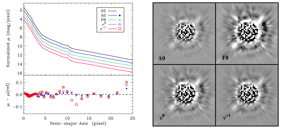
Figure 1: PSF variation as a function of spectral type. (Left) PSFs in the F606W filter created by TinyTim with different SEDs: O5 star (black line, the reference PSF), A0 star (blue line and circles), F8 star (green line and crosses), $F_{\nu}\propto\nu^{0}$ power law (magenta line and diamonds), and $F_{\nu}\propto\nu^{-1}$ power law (red line and squares). The top panel shows the normalized surface brightness profiles (each offset by 0.7 units in the ordinate for clarity) as a function of semi-major axis. The bottom panel shows the residuals of the surface brightness profiles between the reference PSF and the other PSFs. (Right) Residual images of each PSF image after fitting it to the reference PSF. The size of each box is 50$\times$50 pixels ($\sim 5$^′′$\times$5^′′). All images are on a linear gray scale. The variation is almost negligible.

2.1 PSF Variation

PSF variations in HST images can be broadly separated into three categories: color differences due to the spectral energy distribution (SED) of an astronomical object, spatial changes due to optical distortions across the field of view, and temporal changes due to gradual movements of the telescope optical system.

We first compare these three effects to see which of them produces the largest PSF changes.

Color variability      The PSF used in the analysis (e.g., a star) often has a different color than the science target (e.g., an AGN). The color differences may translate into PSF mismatches because HST produces diffraction-limited images. To study this effect, we can use TinyTim PSFs because chromatic differences of light propagation through the telescope optics should be fairly accurately known. We create several non-oversampled PSFs with different SEDs in the F606W filter, which is the widest filter and will have the strongest chromatic PSF variation.

Figure 1 summarizes our results in terms of the average 1-D surface brightness profiles of the models, extracted using the IRAF task ellipse. The variation due to SED is less than 10% at all radii, which is negligible compared to that due to position difference (see below). We also perform the same test with different filters (e.g., F555W and F814W) and find the variation to be still minimal. These results should be robust to the extent that the filter traces and detector responses are well known. We caution, however, that the differences may be more prominent if the filters suffer from red or blue light leaks, such as that seen in the ACS/HRC F850LP filter (Sirianni et al. 2005). Furthermore, we do not suggest that the color effect should be ignored when it is possible to mitigate it in the observations. Its relative importance, however, is small compared to spatial and temporal variability. In general, white dwarf standards like EGGR102 are a reasonable color match to quasar nuclei.

Spatial variability      We create several PSFs, located at different positions on the WF3 detector on WFPC2, again using TinyTim. The one located at the center of the chip, at pixel position ($x,y$) = (400,400), is used as the point of reference. The others are generated at other image positions, with otherwise the same conditions as the reference PSF. It is known that the TinyTim software may not perfectly model real stellar images, in absolute terms, due to light scattering, spacecraft jitter, focus, and other effects. However, external factors largely affect the PSF across the detector uniformly, whereas it is the differential optical distortions due to geometric optics (center vs. outskirts of the field) that concern us here. In general, global field distortions due to geometric optics are both very well known and stable. Even if otherwise, we need not have high accuracy for our purposes. Therefore, the TinyTim synthetic PSFs more than suffice for our goals.

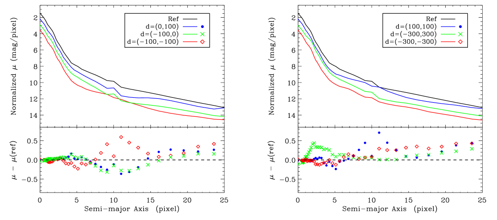
Figure 2: Similar to left panel of Fig. 1, except here we show PSF variations due to position changes. The reference PSF (black line) is located at the center, ($x,y$) = (400,400) of the WF3 detector on WFPC2. The other PSFs are created at different locations, with the following pixel offsets with respect the reference PSF. (Left) ($x,y$) = (0,100) (blue line and circles), ($-$100,0) (green line and crosses), and ($-$100,$-$100) (red line and diamonds). (Right) ($x,y$) = (100,100) (blue line and circles), ($-$300,300) (green line and crosses), and ($-$300,$-$300) (red line and diamonds). As the position offset increases, the discrepancy between the PSFs increases.

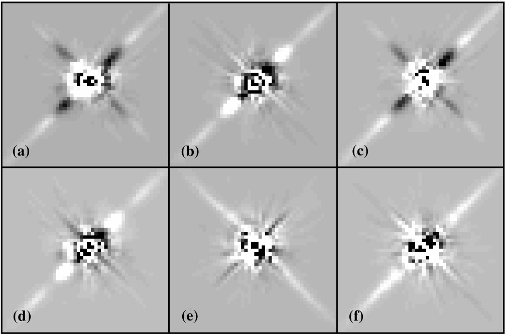
Figure 3: Comparison of the reference PSF with the other PSFs located at different positions described in Fig. 2. We show the 2-D residual images after fitting each PSF to the reference PSF. The pixel offsets with respect to the reference PSF are (a) (0,100), (b) ($-$100,0), (c) ($-$100,$-$100), (d) (100,100), (e) ($-$300,300), and (f) ($-$300,$-$300). The size of each box is 50$\times$50 pixels ($\sim 5$^′′$\times$5^′′). All images are on a linear gray scale. The PSF variation due to position changes is substantial.

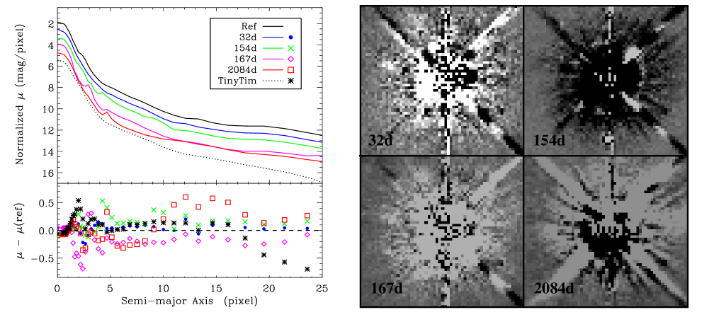
Figure 4: (Left) Similar to Fig. 1, except that here we show PSF variation as a function of time. The reference PSF (black line) was observed on 1995 October 1 with the WF3 detector and the F606W filter. The other PSFs were observed with the same filter and detector 32 days (blue line and circles), 154 days (green line and crosses), 167 days (magenta line and diamonds), and 2084 days (red line and squares) later. We also compare another PSF made with TinyTim (dotted line and asterisks). (Right) Residual images resulting from fitting each PSF with the reference PSF. The size of each box is 60$\times$60 pixels. These results show that temporal variations of the PSF are larger than variations due to spectral changes. All images are on a linear gray scale.

Figure 2 shows that the degree of variation grows with increasing distance from the center of the chip. Spatial variations, at distances separated by less than 100 pixels, affect the wings, but not much the core. In fact, the core appears stable to within 10%, whereas the wings can vary by up to 30%. On the other hand, for PSFs separated by more than 100 pixels, the differences are large both in the wings and in the core, by as much by 30%–50%. Figure 3 visually shows the residuals between each of the PSFs relative to the reference. In light of the systematics observed in Figure 2, it is clear that even if no host galaxy light is detected beneath an AGN, sometimes it is possible to misconstrue its presence, especially in 1-D surface brightness profiles. In 2-D it can be seen that much of the excess flux in the wings at larger radii is due to an imperfect match in the diffraction spikes, which make up a high fraction of the flux locally. From this experiment we conclude that to minimize PSF systematics, it is crucial to find PSF stars that are observed to well within 100 pixels from the reference position of the science target.

Temporal variability      To quantify temporal variability, the PSFs need to be observed in different orbits, so TinyTim is not suitable for this experiment. To obtain PSFs separated in time, we searched in the HST Archive for stars observed with the same detector (WF3) and same filter (F606W), but in different orbits. Our requirement is that they have sufficiently high signal-to-noise ratio ($S/N$) in the wings while being not so bright that they are saturated in the core, and that they are located close to the same chip locations. There are only five stellar images that meet these criteria in the HST Archive. And, while four of the PSF stars were observed in the same HST program and located at the same position, the fifth was placed 90 pixels away. Furthermore, while the observations were done within 5 months for four images, the last one was obtained 6 years later. Therefore, we can test both the short- and the long-timescale variations with these five PSF stars.

We fit all the stars to the reference star, defined here to be that observed at the earliest epoch. We subtracted the sky value for all images before the fit was done. The fit, performed in a region of size $60\times 60$ pixels, contains two free parameters, namely the position and the magnitude of the star. To achieve a PSF image with high dynamic range, we combined a short exposure of the unsaturated core with a long exposure that achieves good $S/N$ in the wings. This procedure still leaves some bleeding columns from the saturated core. The bleeding regions, however, cover only $\sim 1\%$ of the fitting region, and the amplitude of the corrupted pixels is less than $10^{-5}$ (12.5 mag) of the maximum value of the stellar core. Thus, these regions have no quantitative effect on the fit.

Figure 4 shows the 1-D surface brightness profiles and the residual images. In comparison to spatial variations and chromatic issues, the temporal variation is significantly larger and affects the entire PSF, in both the core and the wings. The variation on short timescales ($\sim$ 1 month, circles in Fig. 4) is less than $\pm$0.2 mag, which is slightly less than that in 5 months (crosses and diamonds). However, the star observed 6 years apart (squares) deviates from the reference star by $\pm 0.6$ mag in the full range. Comparing also the TinyTim PSF (asterisks), it is obvious that TinyTim does not do well at modeling either the core or the wings; in particular, it underestimates the flux in the wings. The residual images from the 2-D fit also show that the profile shape systematically changes with time. We note that the PSF star observed $\sim$6 years apart is affected not only by temporal variations but also by spatial variation, being separated by $\sim$90 pixels from the reference star.

2.2 Undersampling of the PSF

In addition to the considerations above, an important issue to bear in mind is that most of images obtained using HST are undersampled from optical wavelengths up to $\sim 1.6\,\mu$m (when observed with the NIC2 camera on NICMOS). The effect of undersampling is most severe for the WF CCDs on WFPC2. Undersampling of the PSF is a problem in high-contrast imaging because fitting the AGN requires matching its centroid to that of PSF image, which involves subpixel interpolation to reassign flux across pixel boundaries. When a PSF is not Nyquist-sampled, the interpolation fundamentally does not have a unique solution, so that subtracting one unresolved source from another introduces a large amount of numerical noise, which severely hampers high-contrast imaging. Lastly, image convolution cannot be performed correctly because of frequency-aliasing in taking the Fourier transforms of the PSF and the host galaxy model.

In the WF camera of WFPC2, the full width at half maximum (FWHM) of the PSF is undersampled at 1.5 pixels in $V$. Therefore, it is not possible to preserve the original shape of the PSF when shifting by a fraction of a pixel. The program GALFIT uses a tapered sinc + bicubic kernel in order to maintain the intrinsic width of the PSF under subpixel interpolation. This method is used because it preserves flux and is significantly superior to linear and spline interpolation in regimes especially near Nyquist-sampling frequencies. However, when an image is undersampled, complications can arise because subpixel interpolation can significantly change both the amplitude and the width of the unresolved flux, while the wings of the PSF, being much better sampled, do not change much. This problem exists independently of, and affects all, the interpolation techniques. The changing of the core-to-wing ratio of the PSF then becomes numerically degenerate with the profile of the host galaxy component beneath.

To illustrate the problem of subpixel shifting qualitatively, we shifted two empirical PSF images by a subpixel unit, here arbitrarily chosen to be 0.3 pixels. As

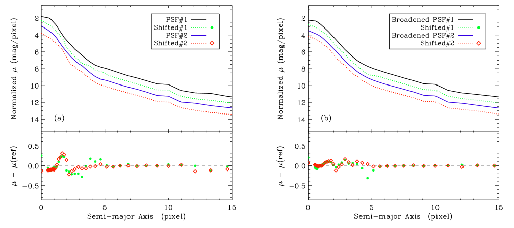
Figure 5: Variation of the PSF from subpixel shifts of the undersampled PSF. Two PSFs are shown, each arbitrarily shifted by 0.3 pixels. (a) Difference between the original PSF and the shifted one for two observed PSFs. Large variations are seen in the central region. The top panel shows the normalized surface brightness profiles (each offset by 0.7 units in the ordinate for clarity) as a function of semi-major axis. (b) We broaden the PSFs using a Gaussian kernel with a FWHM of 2 pixels. The effect of the subpixel shift is now significantly reduced.

shown in Figure 5a, while both the width and the flux in the wings do not change much, the central value changes by 20%–30%. In the outskirts ($>$10 pixels), small differences remain due to the fact that the diffraction spikes are also not Nyquist-sampled. Figure 5b shows the same PSFs when they are broadened to Nyquist sampling. Small differences necessarily remain because the PSF images are shifted first before being broadened, but the agreement is much better. While superficially there appears to be a resolution loss by broadening the PSF in such a way, fundamentally, according to sampling theory, there is no more information content in Figure 5a than there is in Figure 5b if they are used or analyzed as single images. Information content is there to achieve “super”-resolution only when subpixel dithering is used to construct the final images. Figure 5a indicates that even if the PSF image is taken during the same orbit as the host galaxy image, additional errors could be introduced by subpixel interpolation no matter how sophisticated is the method of interpolation. These figures suggest a way to alleviate the problem, which will be discussed in Section 3.4.

In summary, the shape of the PSF is sensitive to changes that occur in time and dependent on the position on the detector, but to a much lesser degree on the SED of the source. More importantly, in terms of temporal variability, these results, with caveats about small number statistics, suggest that even though the telescope cameras undergo refocusing from time to time, cumulative effects build up through time that may not be fully removed by refocusing of the camera alone.

For the remainder of the discussion on the simulations, we will pick two observed PSF stars: the reference PSF star and another that is taken 1 month later and located within 100 pixels of the reference. For these two PSF stars, the difference near the peak is 15% of the maximum, and while systematic differences in the residuals are small, the variance in the central 50 pixels is 4% of the peak value, as seen in Figure 4. Later on, we will also fit the simulations with a TinyTim PSF, to contrast with the results obtained through using observed PSF stars.

3 SIMULATIONS

In the previous section, we identified the factors that most influence the shape of the PSF. We find that it is possible to reduce the systematic differences of the PSFs if certain precautions are taken during the observational stage. Nevertheless, even under the most extreme care, systematic differences will still propagate into the analysis due to the aforementioned effects. For realistic HST observations, it is often impractical to observe PSF stars ideal for all the science data in hand. Therefore, in this section, we seek to quantify the extent that observations are typically affected by performing image-fitting simulations under realistic observational conditions, to the extent that it is possible to mitigate the PSF mismatches a priori. We use GALFIT (Peng et al. 2002) to conduct the simulations. GALFIT is designed to perform 2-D profile fitting and allows us to fit a galaxy image with multiple components convolved with a PSF. Although other 2-D fitting programs exist (e.g., McLure et al. 1999; Schade et al. 2000), the results of this study are sufficiently general that the main conclusions should be broadly applicable to AGN imaging studies in general.

HST observations of AGNs have been obtained using various exposure times, sensitivities, instruments, and filters. The simulations below are intended to be broadly useful for a wide range of past studies using HST as well as future studies, where the image sampling is close to Nyquist sampling. For this reason, we adopt the following strategy in producing the simulations: the simulations are first and foremost referenced to the $S/N$ of the AGN nucleus (defined below). The $S/N$ of the unresolved nucleus is often the easiest parameter to measure in luminous AGNs, and is more general than the luminosity parameter. Secondly, at a given $(S/N)_{\rm nuc}$ in the simulation, the host galaxy flux normalization is referenced to that of the AGN—a quantity that we call the “luminosity contrast” ($L_{\rm host}/L_{\rm nuc}$)—instead of using the absolute luminosity of the galaxy. Luminosity contrast is often the factor that determines the reliability of host galaxy detection: when $L_{\rm host}/L_{\rm nuc}$ is low, it is hard to detect the host galaxy, whereas when $L_{\rm host}/L_{\rm nuc}$ is high, the AGN is harder to measure. Both low and high $L_{\rm host}/L_{\rm nuc}$ are considered to be high contrast. The strategy of using $(S/N)_{\rm nuc}$ and $L_{\rm host}/L_{\rm nuc}$ makes irrelevant information about the exposure time and intrinsic luminosity when quantifying parameter uncertainties of the AGN and the host. Therefore, once the $(S/N)_{\rm nuc}$ and $L_{\rm host}/L_{\rm nuc}$ parameters are measured, uncertainties in the measurement parameters can be estimated by referring to the appropriate figure for a given $(S/N)_{\rm nuc}$.

The $S/N$ of the unresolved nucleus is calculated, without loss of generality, by defining that all the flux is concentrated within a single pixel. Thus,

$$(S/N)_{\rm nuc}=\frac{F_{\rm nuc}}{\sqrt{F_{\rm nuc}+Rd^{2}+Sky+Dark}},$$ (1)

where $F_{\rm nuc}$ is the total flux of the unresolved AGN nucleus, $Rd$ is the readout noise, $Sky$ is the sky value, $Dark$ is the dark current, and all quantities are in units of electrons. The $S/N$ for the nucleus calculated in this manner is slightly larger than the value obtained from that accounting for the fact that the point source has a finite width. However, since the unresolved core is not in the read-noise or sky-dominated regime, and most of the flux is contained within 1 to 2 pixels, the noise of the core hardly depends on the exact area. The advantage of our definition is that it can be easily renormalized to other areas in lower $S/N$ regimes. We note that the main results of this paper are actually not very sensitive to the exact value of $(S/N)_{\rm nuc}$.

3.1 Creation of the Simulation

The reference simulation models were produced using a single reference PSF to represent the AGN nucleus and for image convolution. The light profile of the host galaxy was parameterized as a single-component Sérsic (1968) profile, convolved with the reference PSF. We made 10,000 reference images, by varying the following parameters: (1) $S/N$ of the nucleus [$50\leq(S/N)_{\rm nuc}\leq 5000$] on a logarithmic scale, (2) luminosity ratio between galaxy and nucleus ($0.01\leq L_{\rm host}/L_{\rm nuc}\leq 100$) on a logarithmic scale, (3) effective radius ($1\ {\rm pixel}\leq R_{e}\leq 50\ {\rm pixel}$) on a logarithmic scale, (4) axis ratio ($0.7\leq b/a\leq 1$) on a linear scale, and (5) Sérsic index ($n=1$, equivalent to an exponential profile, or $n=4$, equivalent to a de Vaucouleurs profile). The values were randomly selected in these ranges. The range of values for the host galaxy parameters ($R_{e}$, $b/a$, and $n$) was determined by the typical range seen in actual observations. The size of each simulated image is $\sim$10 times larger than $R_{e}$. To maximize efficiency for the simulations, we use a convolution size of $50\times 50$ pixels for the PSF image; we verified that enlarging the convolution size to $100\times 100$ pixels has no noticeable impact on the results.

To cast the simulations into more concrete terms, the foregoing parameters, translated to single-orbit, 3000-second HST images, mean that the range of $(S/N)_{\rm nuc}$ corresponds to $15\leq m_{\rm F606W}\leq 25$, with the host galaxies spanning $\pm 5$ magnitudes around that range. This sufficiently covers most of the data contained in the HST archive, and the dynamic range is large enough for most practical observations.

The simulations below examine the most typical circumstances encountered in high-contrast images. During the fit, we allow the following sets of parameters to be free: (1) position, luminosity, effective radius, axis ratio, position angle, and Sérsic index for the galaxy; (2) position and luminosity for the nucleus; and (3) sky value.

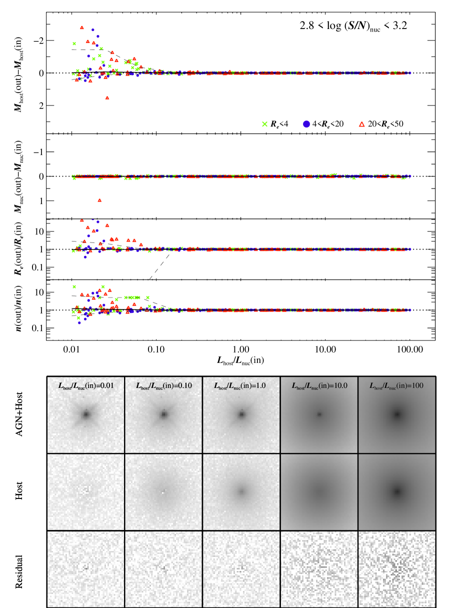
Figure 6: Simulation results under idealized conditions. We fit artificial images with the same PSF as that used for generating the input images. The upper part of the figure shows residuals in the magnitude of the host ($M_{\rm host}$), magnitude of the nucleus ($M_{\rm nuc}$), effective radius ($R_{e}$), and Sérsic index ($n$) as a function of input luminosity ratio between the host and the nucleus ($L_{\rm host}/L_{\rm nuc}$) and input signal-to-noise ratio of the nucleus [$(S/N)_{\rm nuc}$]. Host galaxies of different effective radii are marked in (green, $R_{e}<4$ pixel), (blue, $4<R_{e}<20$ pixel), and (red, $20<R_{e}<50$ pixel). Here, we only show the results for $10^{2.8}\leq$ $(S/N)_{\rm nuc}$ $\leq 10^{3.2}$, which is typical of most actual objects observed with HST. The plots for other values of $(S/N)_{\rm nuc}$ are presented in the Appendix. We plot only 25% of the data points to avoid crowding; this subset of points adequately represents the overall trends. The solid lines represent the median value for the simulated sample, while the dashed lines demarcate the region that encloses the central 70% of the sample. The lower portion of the figure shows examples of the artificial and residual images as a function of increasing $L_{\rm host}/L_{\rm nuc}$ (from left to right). All images are on an asinh stretch.

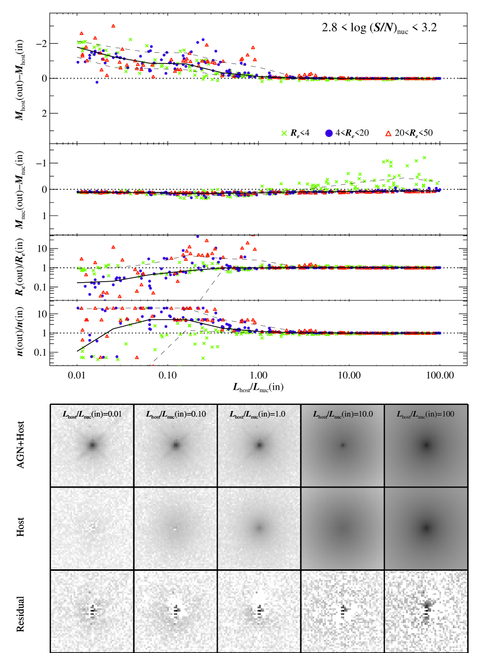
Figure 7: Similar to Fig. 6, except that here we fit the artificial image with a PSF different from the one used for generating the input image. The conditions of the simulation are more realistic than those in Fig. 6. This test shows that PSF mismatch is the main culprit for the systematic uncertainty.

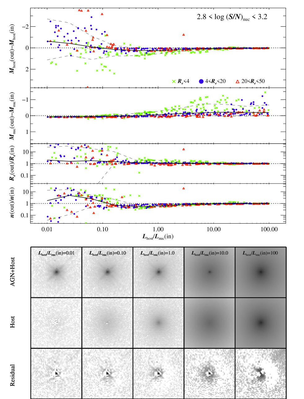
Figure 8: Similar to Fig. 6, except that here the fits were done with the TinyTim PSF, which was not oversampled. The conditions of the simulations are more realistic than those in Fig. 6. This test suggests that the scatter for the host parameters is due to PSF mismatch, but the systematics, except for the nuclear magnitude, seem to be better controlled than in Fig. 7.

3.2 Idealized Simulations

As a point of reference, our first set of simulations is designed to be highly idealized: we fit the artificial images with the same PSF used to create them. Although this simulation does not account for PSF mismatch, it gives us a “zero point” expectation for how well we can extract the host galaxy parameters in the photon limit. The simulation results are summarized in Figure 6, where we show the residual of galaxy luminosity, nucleus luminosity, effective radius, and Sérsic index as a function of the luminosity contrast. The $(S/N)_{\rm nuc}$ of $\sim 1000$ in Figure 6 corresponds to a point source magnitude of 18.5 mag in the F606W filter, for a single HST orbit. In the Appendix, we show plots of other $(S/N)_{\rm nuc}$ regimes. In Figure 6, when the luminosity of the AGN is more than 10 times the host luminosity, the underlying galaxy tends to be dominated by the noise of the nucleus. In this case, GALFIT tries to extract the host galaxy component from the nucleus itself, which leads to the Sérsic component having a smaller size and a higher Sérsic index. The size of the galaxy is also important. When $R_{e}$ is small (green dots) and difficult to distinguish from the nucleus, or large (red dots) and has low surface brightness, the scatter in all morphology parameters is large. However, we find that the scatter is not very dependent upon the Sérsic index of the host galaxy. Most importantly, when the AGN is brighter than 20:1, the host galaxy detection becomes quite difficult even under ideal conditions. This is similar to findings in nearly all quasar host galaxy studies where the hosts are often not much fainter than 3 magnitudes compared to the AGN. Under certain situations it is possible to detect quasar hosts that have a higher contrast with the AGN, such as when the host has a high ellipticity (and thus a high surface brightness). In these limits, the fluxes of even real host detections are likely to be biased systematically high.

3.3 Testing PSF Mismatches

To test PSF mismatches we fit the simulated data with a different PSF from the one that was used to create them. We first test the results by fitting with a stellar PSF, and next with a model PSF generated by TinyTim.

Stellar PSF.     In this simulation the analysis PSF (FWHM $\approx 1.6$ pixels) was observed one month apart from that (FWHM $\approx 1.5$ pixels) used to generate the 10,000 reference data models. This experiment is more realistic because most AGN observations do not have concurrently observed PSFs; they rely instead on PSFs in the archive or TinyTim models.

The simulations (Fig. 7) show that even when the PSF matches are fairly good, as seen in the residual images, the systematic errors can be quite large. When the contrast is high, the effective radius and Sérsic index plots show that GALFIT may try to reduce the PSF mismatch by using the host galaxy Sérsic component, the result of which is to push the concentration index to either extreme and to make the galaxy size small. The host galaxy luminosity robs light from the quasar itself in the process. For compact galaxies, the systematic errors start to increase around $L_{\rm host}/L_{\rm nuc}$$\approx 1$. For low-surface brightness galaxies ($R_{e}>20$ pixels), the errors occur at higher $L_{\rm host}/L_{\rm nuc}$. We note that GALFIT does not permit Sérsic indices larger than $20$, which is why the ratio of the Sérsic indices saturates at a value of 5 [when $n$(in) = 4] or 20 [when $n$(in) = 1].

We further find that the systematic trend is slightly dependent on the Sérsic index, in the sense that the hosts with $n$(in) = 1 is better recovered than those with $n$(in) = 4, but less so when $(S/N)_{\rm nuc}$ $\mathrel{\hbox{\hbox to0.0pt{\hbox{\lower 4.0pt\hbox{$\sim$}}\hss}\hbox{$>$}}}$ 250. When the host has an $n=4$ profile, the recovered flux from the host can be easily buried under the structure of the PSF mismatch. Thus, it is hard to accurately detect an AGN host with a high Sérsic index (central concentration) and small size. At moderate to high $(S/N)_{\rm nuc}$, there is only a small dependence on $(S/N)_{\rm nuc}$ because the systematics are dominated by the PSF mismatch.

As seen in Figure 7, there is a clear offset ($\sim 0.1$ mag) in the luminosity of the nucleus. As explained above (§2.2), and as shown later in §3.4, this effect is caused by the undersampling of the PSF, so that the cores cannot be adequately sampled and modeled. This then leads to an overestimate or underestimate of the halo of the PSF, which results in erroneous inferences on the host galaxy properties when the galaxy is faint. In our case, the underestimate of the nuclear flux boosts the flux of either the sky or the host luminosity. We discuss later in §3.4 how this systematic error can be reduced.

TinyTim PSF.     In addition to fitting the artificial images with an actually observed PSF star, we also tried using a PSF generated with TinyTim (Fig. 8). When there is no stellar PSF observation, this is an often-used strategy in the literature. We create a 1$\times$ sampled PSF for this analysis. Figure 8 shows that the fit with this synthetic PSF is less accurate compared to the previous two simulations using an observed star. In particular, if the size of the host galaxy is small, the parameter recovery is quite poor, even if the residuals may not indicate there to be an obvious sign of a PSF mismatch, especially at low $L_{\rm host}/L_{\rm nuc}$. This point cannot be over-emphasized.

Since the TinyTim PSF is sharper than the stellar PSF, the mismatch in the central few pixels is more problematic due to undersampling. As in the previous simulation, when $L_{\rm host}/L_{\rm nuc}$ is large, the AGN flux is measured to be too luminous, even though the host luminosity is not affected much. Therefore it is hard to get accurate fits for both the host and the nucleus simultaneously at the extreme ends of the luminosity contrast if one uses a non-oversampled TinyTim PSF.

We also fit the simulated images with a $4\times$ oversampled TinyTim PSF. When an oversampled PSF is created by the TinyTim program, it is not convolved with a charge diffusion kernel. We manually convolved the oversampled PSF with the charge diffusion kernel. We find no significant differences from the fits with a non-oversampled TinyTim PSF.

3.4 Broadening the PSF and Science Images

To minimize interpolation errors, we need to model both the gradient and the curvature of the PSF, which is not possible when the PSF is undersampled. As discussed in § 2.2, interpolation errors necessarily occur when an undersampled PSF is shifted by a fraction of a pixel, regardless of the algorithm used in the interpolation. To see if this crucial problem can be reduced, we repeated the same simulations by slightly broadening both the PSF star and the simulated images as they are observed. To achieve Nyquist-sampling, we want the final PSF to have a FWHM of 2 pixels. Since the FWHM of the original PSF is $1.5-1.6$ pixels, we use a Gaussian kernel with FWHM = 1.45 pixels for broadening.

As shown in Figures 9 and 10, the results improve considerably. While the behavior of the systematic errors on the host galaxy luminosity is consistent with previous results in Figures 7 and 8, the upturn point ($L_{\rm host}/L_{\rm nuc}$$\approx 0.5$) where GALFIT begins to overestimate the host galaxy luminosity is a factor of 2 less than previously ($L_{\rm host}/L_{\rm nuc}$$\approx 1.0$). This experiment also recovers the luminosity of the nucleus much better than before, even if the host galaxy is small. In addition, the artificial offset in the residual of the AGN luminosity is virtually eliminated. Lastly, the scatter in the fitted parameters has, in all cases, decreased quite substantially.

Interestingly, the improvements for a broadened TinyTim PSF are more dramatic (compare Fig. 10 with Fig. 8), such that a TinyTim PSF can sometimes work better than a real star. The latter fact is probably just a coincidence and not likely to be true in general due to the temporal variability of real PSFs. Nevertheless, the improvement does suggest that if there is no stellar PSF observed, TinyTim can be an acceptable substitute, if both the PSF and the data images are oversampled in the same way. Comparing Figure 10 with Figure 9, in which the fit was done with the broadened stellar PSF, we can conclude that the recovery for host magnitude is reasonable, but the AGN luminosity may still be somewhat biased when the host galaxy is much more luminous.

In summary, the results of these tests indicate that image decomposition should be performed only on images that are Nyquist-sampled. If both the PSF and the data are not sampled adequately, one can simply convolve both images with the same Gaussian kernel. Alternatively, dithering can be used to achieve Nyquist sampling when observing the data and the PSF images.

3.5 Holding the Sérsic Parameter Fixed

When the host galaxies are faint and hard to deblend from their central AGN, one common technique used in the literature is to hold the Sérsic index $n$ fixed, while allowing other parameters to converge (e.g., Jahnke et al. 2004; Sánchez et al. 2004). We perform similar experiments to test how reliably we can extract the host parameters by using such a prior. We create artificial images for $(S/N)_{\rm nuc}$ $=1000$, varying $n$ from 0.8 to 6.8. We only run simulations in the regime where $L_{\rm host}/L_{\rm nuc}$$\approx 0.3$ and $R_{e}=7$ pixels, as this is the part of the host galaxy parameter space where the systematic uncertainties are largest. Fits are performed in four different ways: fixing $n$ = $1$, fixing $n$ = $4$, fixing $n$ to the input value, and allowing $n$ to be free.

Figure 11 summarizes the results. For simulated galaxies where the input Sérsic indices are $n\geq 2$, the luminosity can be recovered to better than 0.3 mag by simply holding the fitted profile to $n=4$ (filled blue circles). This is considerably better than the results that allow the Sérsic index to be free (stars). In addition, if the intrinsic Sérsic index of the host is $n<2$, then holding the fit to $n=1$ also produces a result that agrees to better than 0.3 mag. Therefore, like previous studies, we find that by using a correct prior, the recovery of other host galaxy parameters can dramatically improve. The caveat, however, is that the prior may be hard to determine when the host is not well-resolved. Nevertheless, as the bimodality decision is quite coarse, the decision about which prior to make can in some cases be simply based on selecting the lower of the two $\chi^{2}$ values.

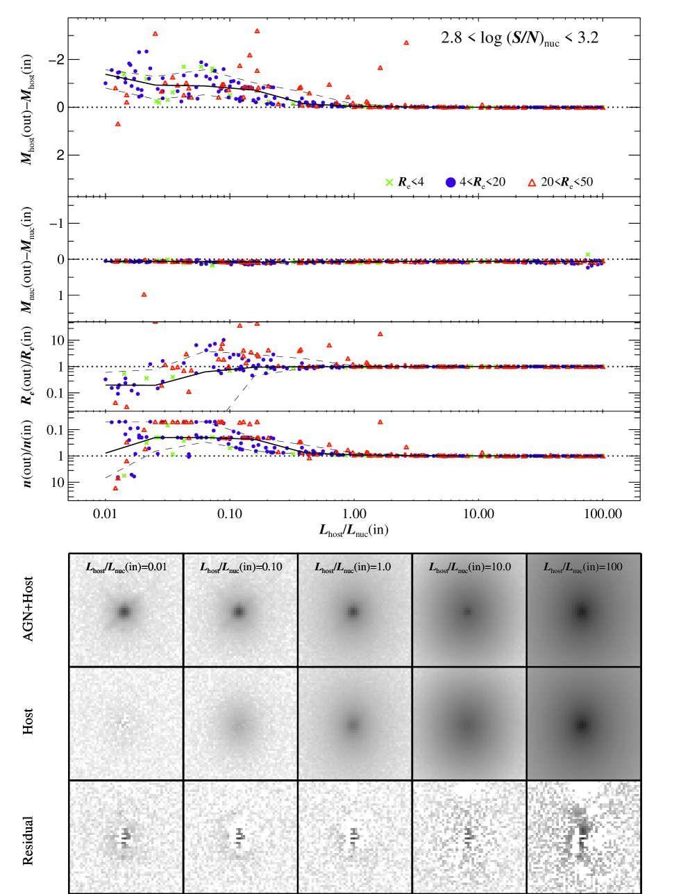
Figure 9: Similar to Fig. 7, except that here we generated the artificial image with an empirical PSF broadened by a Gaussian with FWHM = 2 pixels, and the fits were done with a different, similarly broadened PSF. The input parameters, especially the AGN luminosity, are recovered better than in Fig. 7.

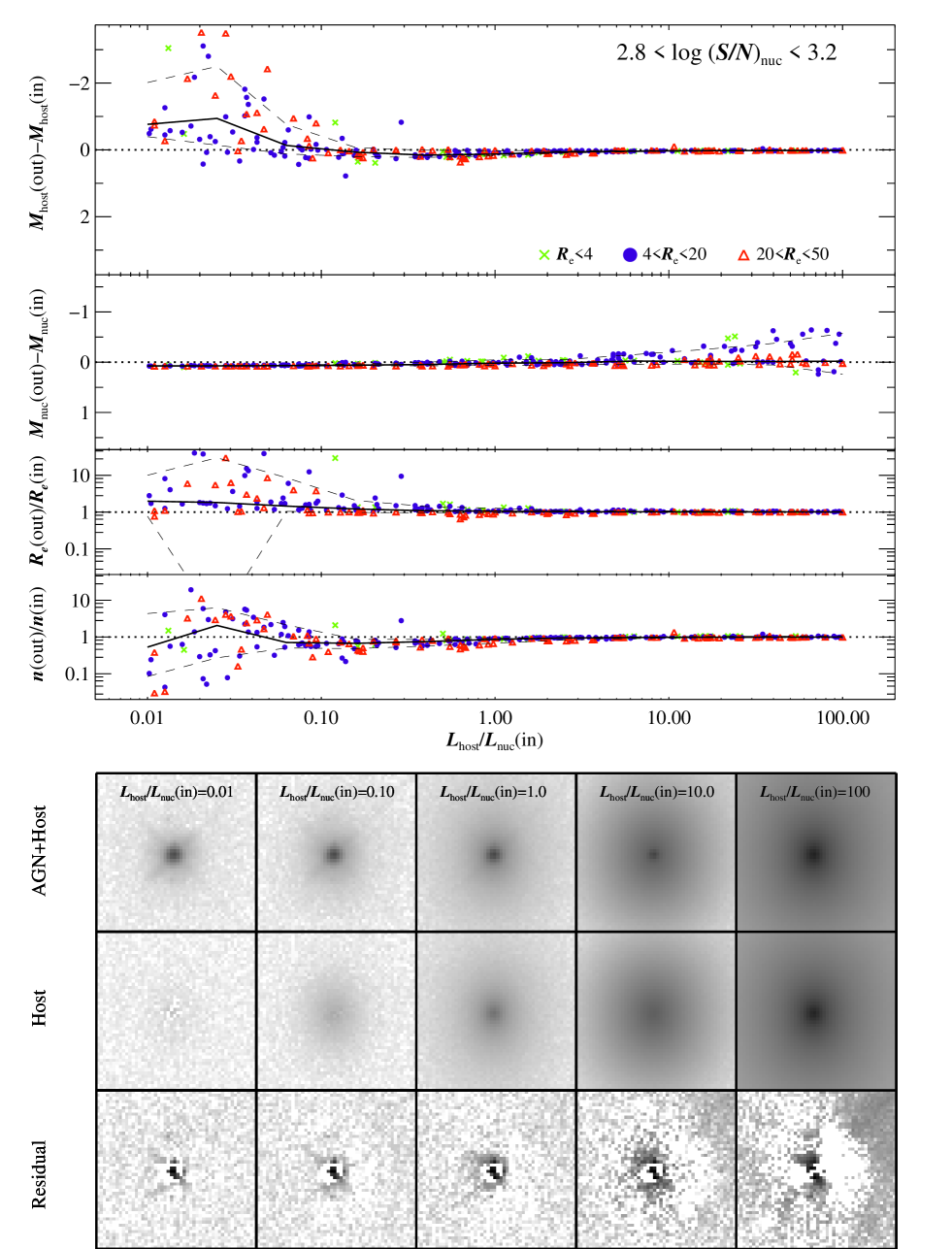
Figure 10: Similar to Fig. 9, except that here we generated the images with a broadened empirical PSF and fitted them with a broadened TinyTim PSF. The recovery of the parameters, especially the AGN luminosity, is substantially improved compared to Fig. 8.

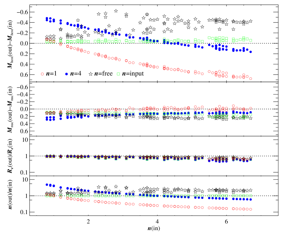
Figure 11: Fitting results with the Sérsic index fixed. After we created artificial images with $n$ varying from 0.8 to 6.8, we fit them in four different ways: fixing $n$ = 1 (open red circles), fixing $n$ = 4 (filled blue circles), fixing $n$ to the input value (green squares), and allowing $n$ to be free (stars). For $n>2$, fixing $n$ = 4 better recovers the input parameters.

3.6 Reversing the Role of the PSFs

Previously, our simulation models were created using a single PSF that has FWHM $\approx$ 1.5 pixels, but which is then fitted using another with FWHM $\approx$ 1.6 pixels. This resulted in systematic biases on the host and AGN parameters in a certain direction. A natural follow-up is to reverse the role of the PSFs to see how the systematic trends may change. As in Figures 7–10, we only show results for $R_{e}<20$ pixels and $10^{2.8}<$$(S/N)_{\rm nuc}$$<10^{3.2}$. Figure 12 shows the results of this set of simulations. We again find that the recovered hosts appear slightly overluminous, but the systematic errors are smaller than the original experiment. Just like before, we find that hosts with $n=1$ and $R_{e}>4$ pixels tend to be recovered well, and the scatter of both the nuclear luminosity and host luminosity are larger when the hosts are small. Even though the degree of systematics is slightly changed, reversing the roles of the PSFs does not affect the systematic error offsets in exactly the opposite direction.

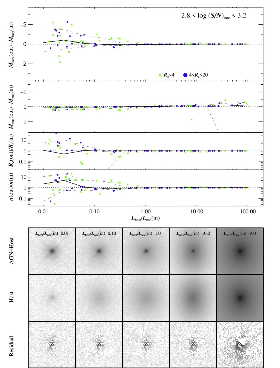
Figure 12: Similar to Fig. 7, except that here we switched the role of the two PSFs used for generating the artificial image and for doing the fit. For simplicity, we only simulate galaxies having $R_{e}<20$ pixels. The overall trends are very similar to those in Fig. 7.

Figure 13a: Simulation results for the ACS/HRC. The overall trends are quite similar to those for WF3 on WFPC2. See Fig. 6 for details.

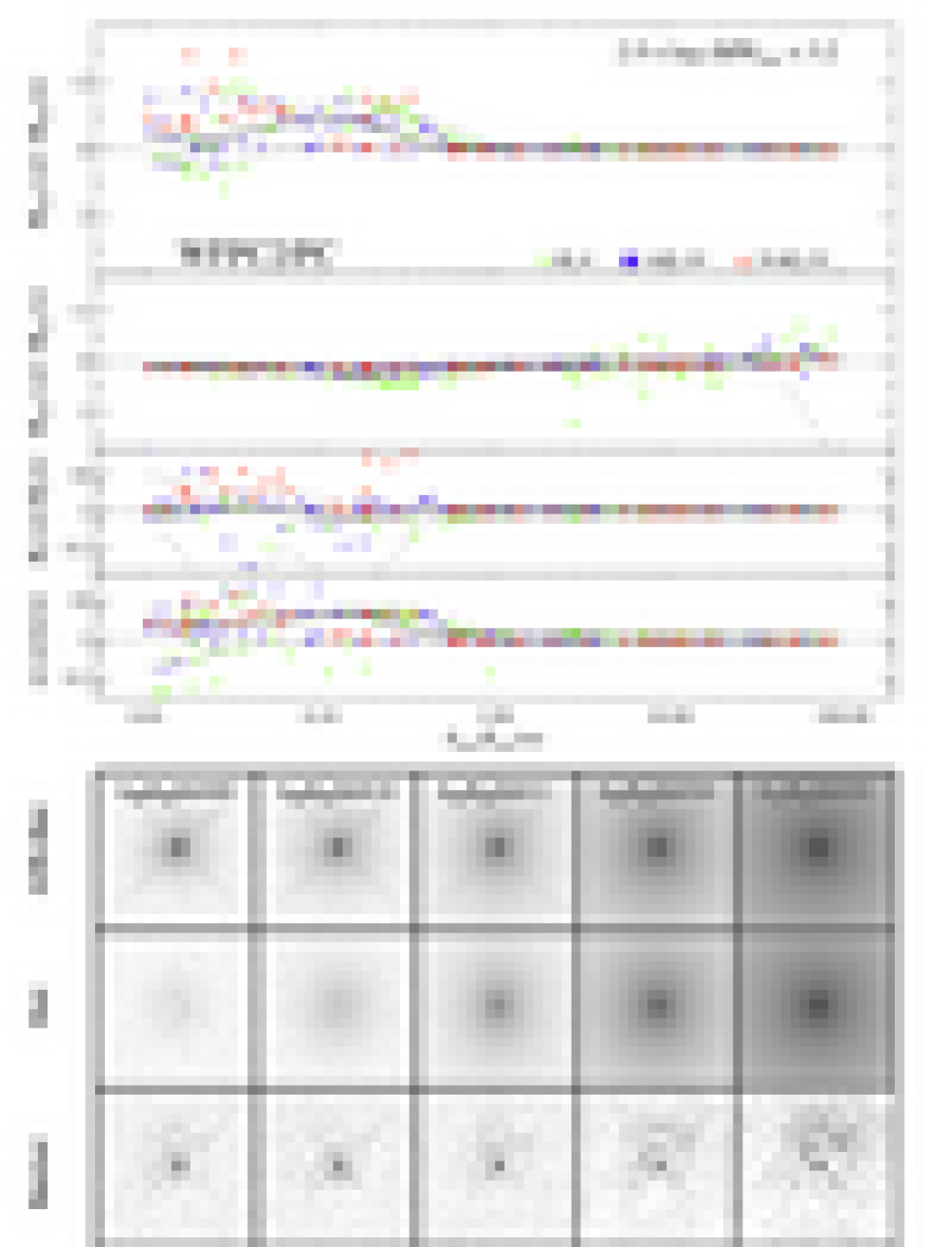
Figure 13b: Simulation results for ACS/WFC. The overall trends are quite similar to those for WF3 on WFPC2. See Fig. 6 for details.

Figure 13c: Simulation results for NICMOS/NIC2. The overall trends are quite similar to those for WF3 on WFPC2. See Fig. 6 for details.

Figure 13d: Simulation results for the WFPC2/PC. The overall trends are quite similar to those for WF3 on WFPC2. See Fig. 6 for details.

3.7 Simulating Other Detectors Onboard HST

Different detectors onboard HST have different characteristics, and so we further perform simulations for each of them. As before, for each detector we use two different stellar PSFs to account for the PSF mismatch. For simplicity, the simulations are done with 1000 samples for $10^{2.8}<$$(S/N)_{\rm nuc}$$<10^{3.2}$. The detectors assumed are the Planetary Camera (PC) of WFPC2, the High Resolution Camera (HRC) of the Advanced Camera for Surveys (ACS), the Wide-Field Camera (WFC) on ACS, and NIC2 of Near-Infrared Camera and Multi-Object Spectrometer (NICMOS). These are the most often-used detectors for AGN imaging. Figure 13 illustrates that, although the results for the various detectors are slightly different, the overall trends are similar to those of WF3. As shown in the previous experiments (Fig. 7), at $L_{\rm host}/L_{\rm nuc}$$<1$ the host luminosities are systematically overestimated due to the PSF mismatch, and the nuclear luminosities tend to be underestimated due to the undersampled PSF. Not surprisingly, the nuclear luminosities are well recovered in the experiments with NIC2 because it has the least undersampled PSF (FWHM $\approx$ 2 pixels). We also perform the same test with reversing the role of PSFs as discussed in §3.6. The overall trends barely change, although the scatter is slightly affected by this test.

3.8 Complications

In addition to the situations presented above, additional complications involve extracting hosts beneath saturated AGNs or performing bulge-to-disk decomposition on AGN hosts. However, characterizing parameter uncertainties in these situations, with considerably larger parameter spaces, is beyond the scope of this study. Nevertheless, we conduct a brief simulation to test how well the parameters can be recovered under very specific circumstances corresponding to single-orbit, WF3 data, with $(S/N)_{\rm nuc}$ $\approx 1000$. The simulations below are otherwise created exactly like previous ones, with the reference PSFs being different than the one used to fit the model images, which are Nyquist-sampled.

Saturated AGN.     To test instances when the AGN is saturated, we mask out the central few saturated pixels in the artificial images. We create a set of artificial images with the Sérsic indices of the host varying from $n=1$ to $n=6$. With the nucleus masked out, there is little leverage to reliably determine the host galaxy central concentration. We thus hold the Sérsic index of the host galaxy fixed to $n=4$ to fit the images. In so doing, we find that the resultant luminosity extracted for the host galaxy has a scatter that is 0.2 mag larger compared to the unsaturated cases. However, with the exception of the scatter, the overall distributions from both tests are in good agreement.

One can achieve high-dynamic range imaging of AGN hosts without saturating the core by combining a short exposure of the center with a long exposure of the outskirts of the galaxy. In this circumstance, however, the noise properties across the image will not be uniform, a situation not captured in our simulations. Nevertheless, as we have shown, the systematic errors of the fits are almost always dominated by PSF mismatch rather than by Poisson noise.

Bulge-to-disk-to-AGN Decomposition.     Characterizing measurement uncertainties of bulge-to-disk-to-AGN (B/D/A) decomposition involves an additional 7 free parameters, if the bulge is a Sérsic profile and is an independent component. This set of simulations again corresponds to $(S/N)_{\rm nuc}$ $\approx 1000$; B/D/A decompositions can only be done on objects with high $S/N$. In the interest of characterizing the uncertainties in measuring the bulge component in isolation, we create two sets of artificial images. The first corresponds to a set of pure bulges that we define as the control sample, for which we only do a bulge-to-AGN (B/A) decomposition. The second set takes the same bulges, around which we assign an exponential disk. In so doing, uncertainties in bulge measurements from the B/D/A decomposition can be directly compared with the control sample of B/A decomposition.

For the bulge components, the Sérsic indices lie in the range $1\leq n\leq 6$. The reference disk models are pure exponentials and have the following parameters: disk scalelength $(1.5-6)\,R_{e}$ and disk luminosities $(0.2-7)\,L_{\rm bul}$. To fit the model images, we fix $n=4$ for the bulge and $n=1$ for the disk. In so doing, we find that the measurement errors for the bulge luminosity for both samples are comparable (Fig. 14) when the bulges have intrinsic Sérsic indices $n\gtrsim 2$. On the other hand, if the spheroid is inherently a pseudobulge (Kormendy & Kennicutt 2004), where $n$ is smaller than 2, the extracted bulge luminosity is significantly overestimated by roughly 0.4 mag. Also, this test sometimes leaves substantial outliers ($\geq 0.5$ mag). The overall scatter in the bulge luminosity is 0.18 mag for the control sample of pure bulge systems, whereas the scatter grows to 0.28 mag for the later-type galaxies that have both a bulge and a disk. Thus, we conclude that the measurement error for the bulge luminosity increases by 0.1 mag in cases

Distribution of residuals for the bulge magnitudes. Here we show the fitting results for pure bulge systems (hatched histogram) with the median value marked with a dotted line. The later-type galaxies that contain both a bulge and a disk are plotted as an open histogram, and their corresponding median value is marked with a dashed line.

where B/D/A decomposition is required.

4 Discussion

In this study, we performed 2-D image-fitting simulations of AGN hosts to illustrate how systematics in the PSF mismatch may affect the deblending of the AGN and the host galaxy components. Based on these simulations, we suggest practical strategies for how to observe and analyze host galaxies with bright active nuclei.

As seen in Figures 6–7, careful determination of the PSF is needed to extract very high-contrast subcomponents accurately. This point was also underscored in the study of Hutchings et al. (2002). We find that the three factors that most affect PSF structures are spatial distortion, temporal changes, and pixel undersampling. The SED of the PSF matters to a much lesser degree, but it is worthwhile to match it when possible. The spatial variation can be reduced by observing a stellar PSF at the same position as the science images. However, the temporal variance is trickier to avoid without observing PSFs concurrently with the science data, which is observationally expensive and rarely done in practice. Even then, some temporal variability may happen even within a single orbit. Nevertheless, as there is evidence that PSF mismatch grows over time, and may not be completely periodic in nature, it is important to obtain a stellar PSF as close in time as possible to the science images. From our tests (§2.1), we recommend that stellar PSF images be taken within a month of the science images. In the absence of a well-matched stellar PSF, synthetic PSFs generated with TinyTim are adequate substitutes (compare Fig. 10 to Fig. 7 and Fig. 9).

In all scenarios, whether using stellar or TinyTim PSFs, both the science image and the PSF image should be oversampled to reduce errors caused by pixel undersampling and subpixel shifting. This can be accomplished by observing the science image and the PSF star using a four-point “dither” pattern to recover finer pixel sampling. Or, if this option is not available, then simply broadening the images through convolution during the analysis stage is an acceptable alternative solution, and certainly better than no treatment at all (§3.4 and Fig. 10).

Figure 15: Distribution of residuals for the magnitudes of the host for (left) $L_{\rm host}/L_{\rm nuc}$$\geq 0.2$ and (right) $L_{\rm host}/L_{\rm nuc}$$<0.2$. After producing artificial images by varying $n$ between 2 and 6, we fit them with $n$ fixed to 4. This simulation gives an estimate of the measurement error for the bulge luminosity.

When the host galaxies are faint and difficult to fit, it may be useful to hold the Sérsic index fixed to a constant value of either $n=1$ or $n=4$. The decision about what value to use might be based on visual morphology, or by comparing $\chi^{2}$ values of the bimodal priors. A similar conclusion was reached by McLure et al. (1999), Jahnke et al. (2004), and Sánchez et al. (2004) in their analysis of quasar host galaxies. By varying the Sérsic index between $n$ = 2 and $n$ = 6, we find that the scatter is $\sigma\approx 0.3$ mag for $L_{\rm host}/L_{\rm nuc}$$\geq 0.2$ and $(S/N)_{\rm nuc}$ $\approx 1000$ (Fig. 15). At higher contrast, $L_{\rm host}/L_{\rm nuc}$$\leq 0.2$, the scatter increases to $\sigma\approx 0.4$ mag.

Lastly, we briefly conducted a three-component bulge/disk/AGN decomposition to characterize uncertainties in estimating the bulge component. We find that when the $S/N$ is high, the contrast is sufficiently low, and the bulges are sufficiently well-resolved, then a B/D/A decomposition can yield reliable bulge luminosity measurements. These simulations are fully compatible with images of $z\lesssim 0.3$ quasar host galaxies (e.g., McLure & Dunlop 1999). Our tests suggest that, when three-component decomposition is required, the uncertainty in the bulge luminosity increases by an additional $\sim$0.1 mag compared to fits without a disk component.

Finally, we note in passing that our simulations allow the sky value to vary during the fitting. For the current application, this choice makes little difference because the images have a large sky area and the profiles are idealized. However, in real science images, the situation will be different. From prior experience with actual HST data, keeping the sky value fixed prevents the Sérsic index from going up to extremely high values in situations where the light profile of the galaxy is not well represented by the Sérsic function. Thus, we recommend keeping the sky parameter fixed to a well-determined value whenever possible.

Appendix A Simulation Results as a Function of $(S/N)_{\rm nuc}$

Here we examine how the fitting results depend on the $S/N$ of the nucleus. Figures 16–18 show the simulation results as a function of $(S/N)_{\rm nuc}$. We divide the sample into 6 bins in $(S/N)_{\rm nuc}$ and 3 bins according to the PSF used for the fit.

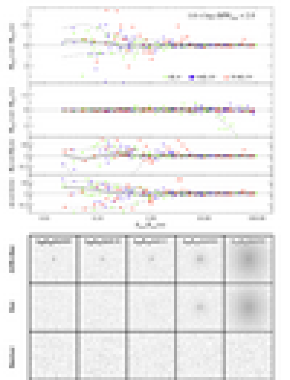
Figure 16a: Simulation results for the idealized situation in which the fitting PSF is identical to that used for generating the input images; see Fig. 6 for details. We display $10^{1.6}\leq$ $(S/N)_{\rm nuc}$ $\leq 10^{2.0}$.

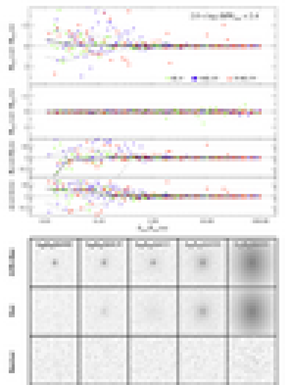
Figure 16b: Simulation results for $10^{2.0}\leq$ $(S/N)_{\rm nuc}$ $\leq 10^{2.4}$.

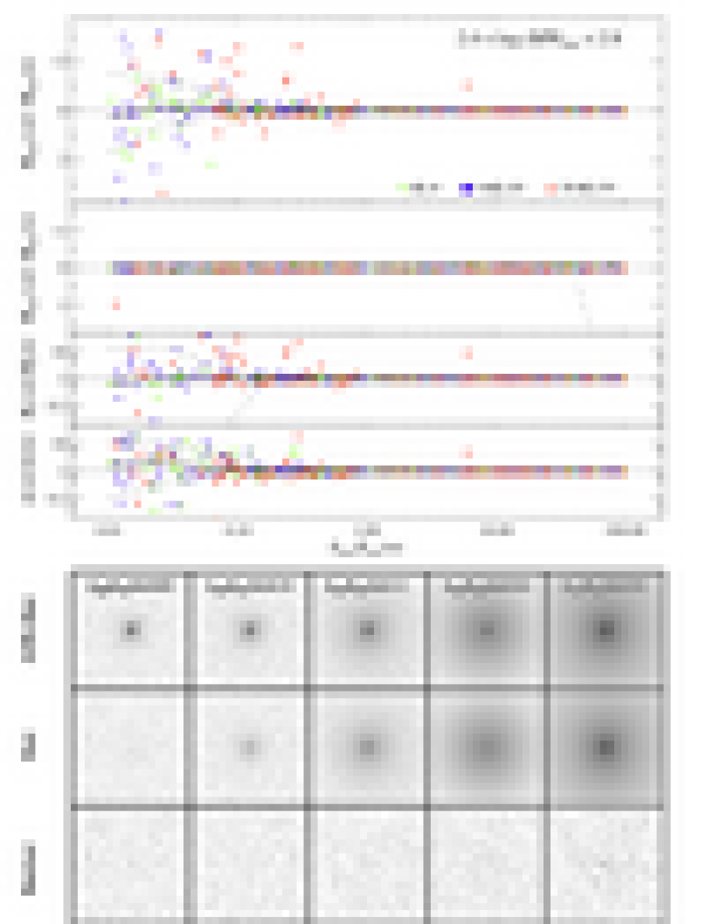
Figure 16c: Simulation results for $10^{2.4}\leq$ $(S/N)_{\rm nuc}$ $\leq 10^{2.8}$.

Figure 16d: Simulation results for $10^{2.8}\leq$ $(S/N)_{\rm nuc}$ $\leq 10^{3.2}$.

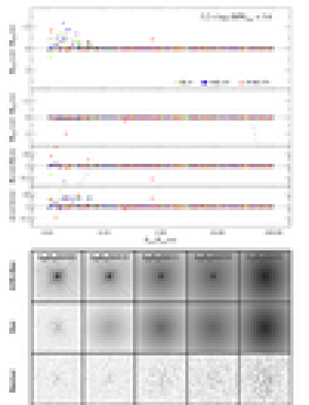
Figure 16e: Simulation results for $10^{3.2}\leq$ $(S/N)_{\rm nuc}$ $\leq 10^{3.6}$.

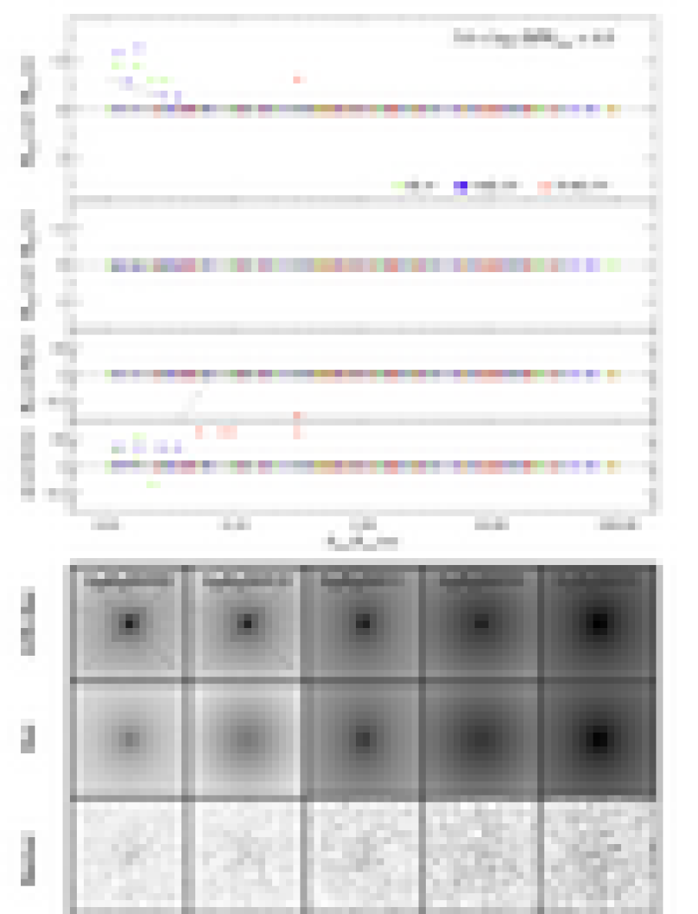
Figure 16f: Simulation results for $10^{3.6}\leq$ $(S/N)_{\rm nuc}$ $\leq 10^{4.0}$.

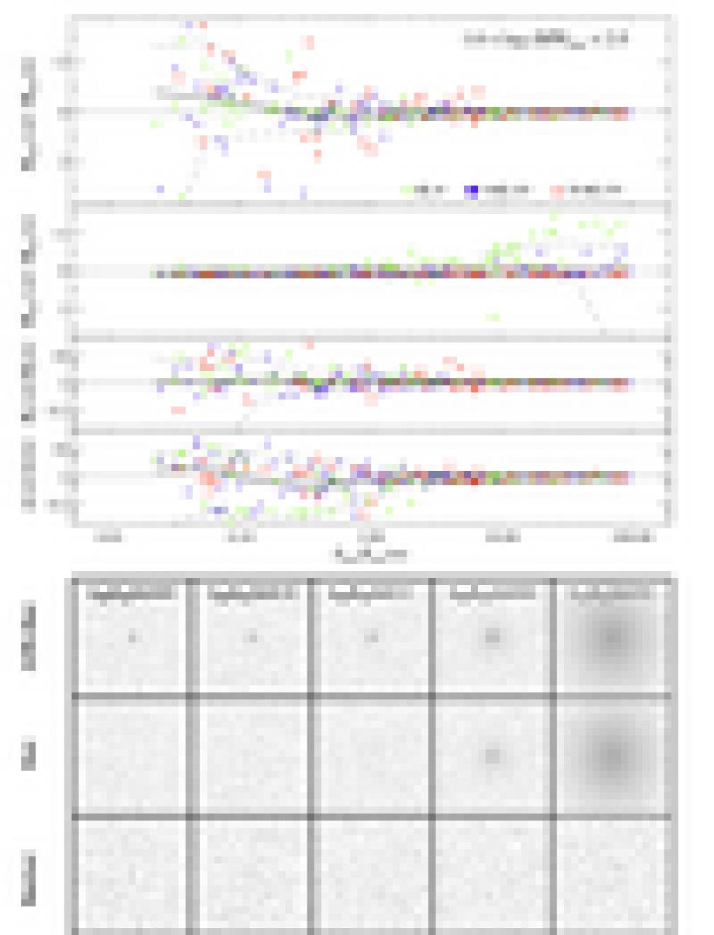
Figure 17a: Similar to Fig. 16a, except that here we fit the artificial images with a PSF different from the one used for generating the input images; see Fig. 6 for details. We display $10^{1.6}\leq$ $(S/N)_{\rm nuc}$ $\leq 10^{2.0}$.

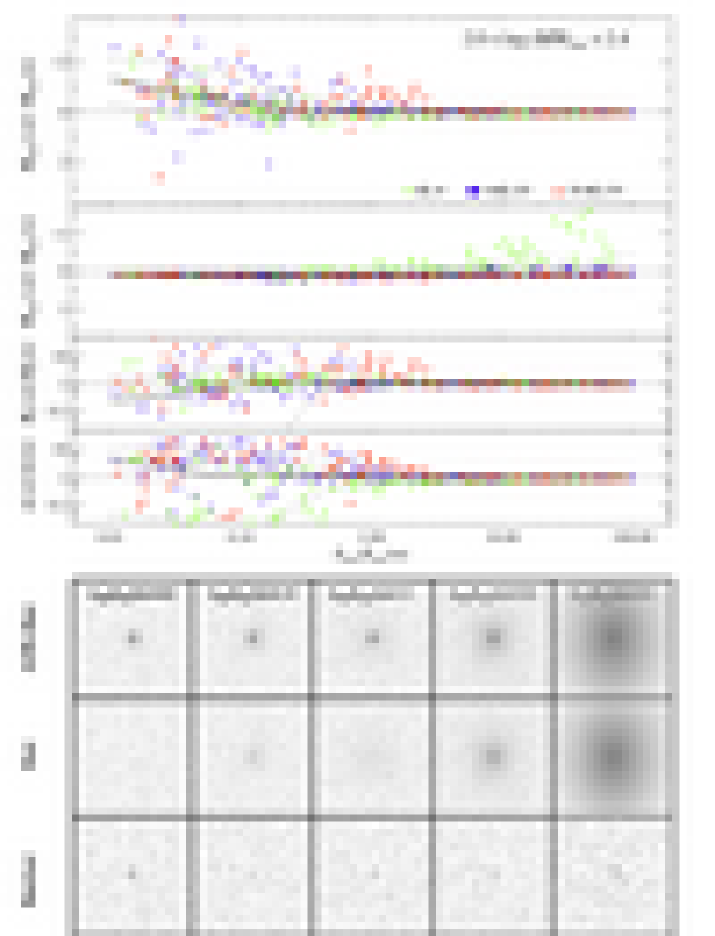
Figure 17b: Simulation results for $10^{2.0}\leq$ $(S/N)_{\rm nuc}$ $\leq 10^{2.4}$.

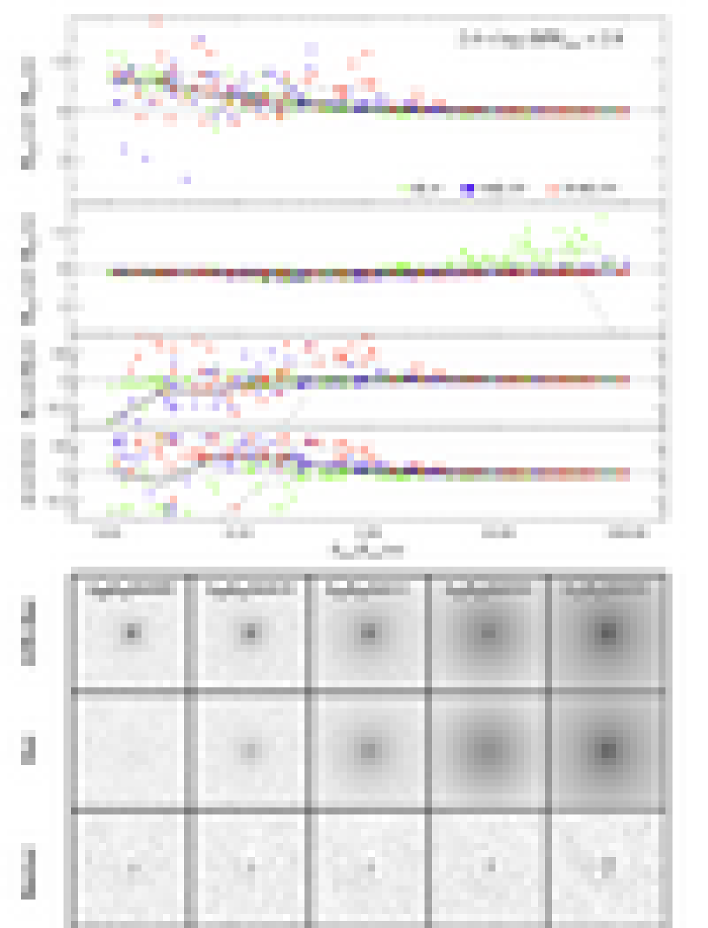
Figure 17c: Simulation results for $10^{2.4}\leq$ $(S/N)_{\rm nuc}$ $\leq 10^{2.8}$.

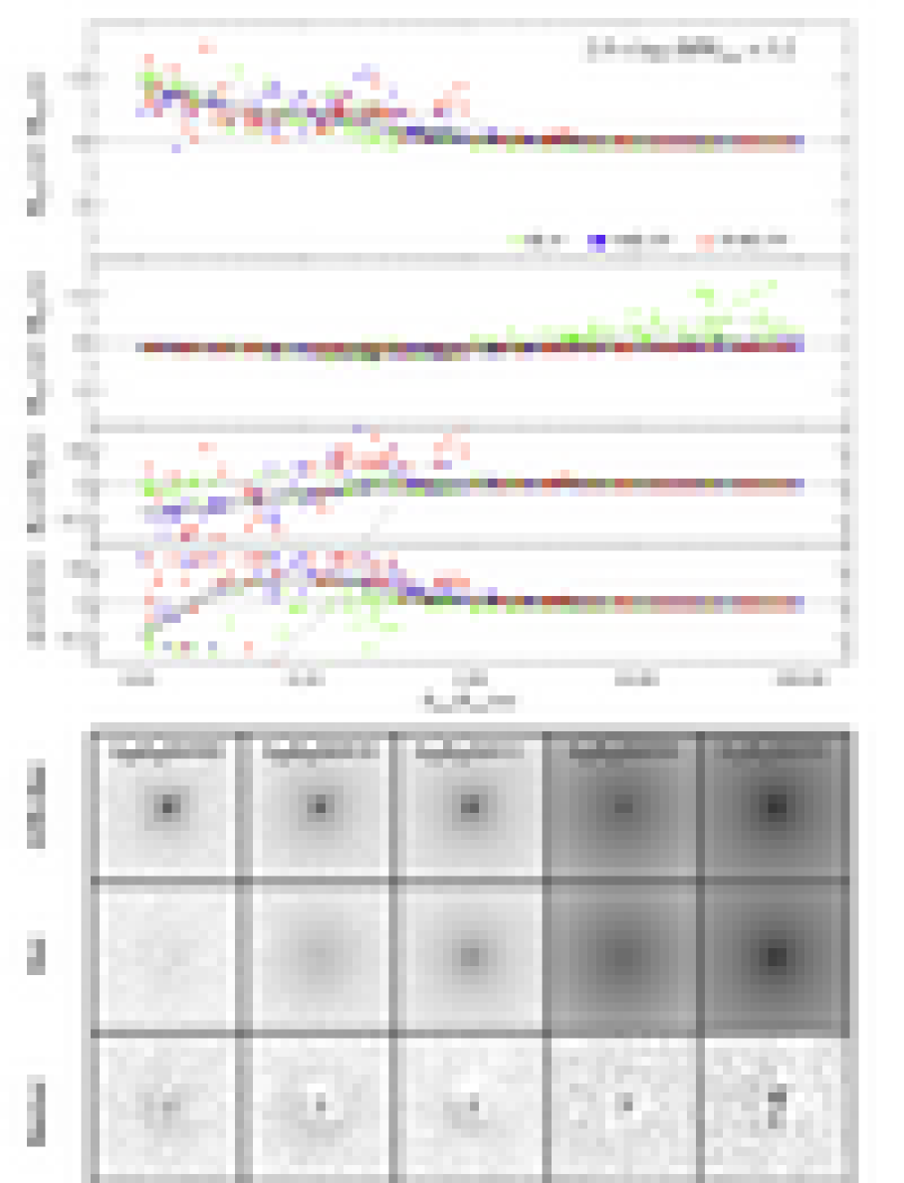
Figure 17d: Simulation results for $10^{2.8}\leq$ $(S/N)_{\rm nuc}$ $\leq 10^{3.2}$.

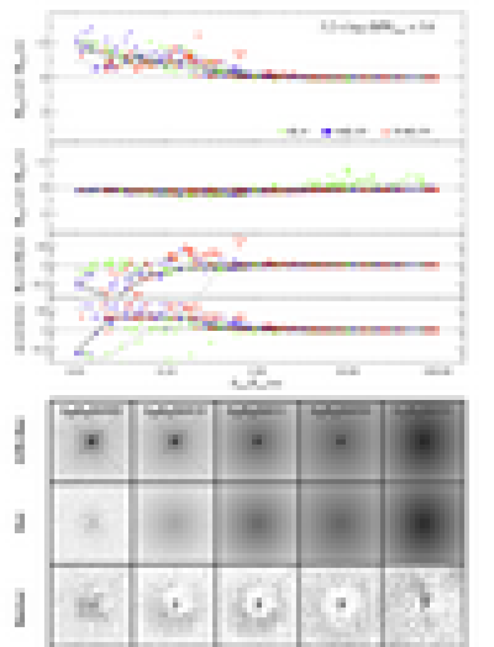
Figure 17e: Simulation results for $10^{3.2}\leq$ $(S/N)_{\rm nuc}$ $\leq 10^{3.6}$.

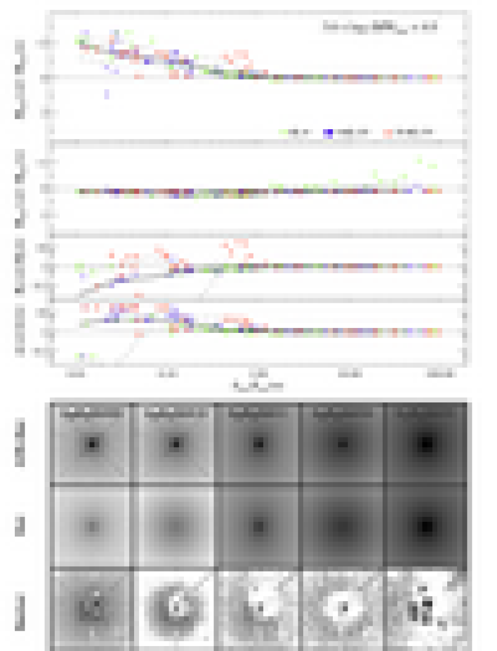
Figure 17f: Simulation results for $10^{3.6}\leq$ $(S/N)_{\rm nuc}$ $\leq 10^{4.0}$.

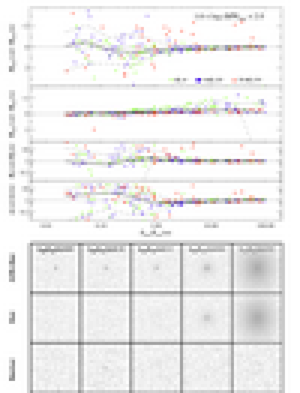
Figure 18a: Similar to Fig. 16a, except that here we fit the images with the TinyTim PSF; see Fig. 6 for details. We display $10^{1.6}\leq$ $(S/N)_{\rm nuc}$ $\leq 10^{2.0}$.

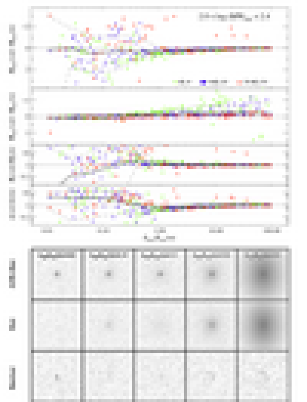
Figure 18b: Simulation results for $10^{2.0}\leq$ $(S/N)_{\rm nuc}$ $\leq 10^{2.4}$.

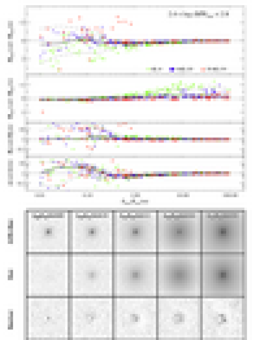
Figure 18c: Simulation results for $10^{2.4}\leq$ $(S/N)_{\rm nuc}$ $\leq 10^{2.8}$.

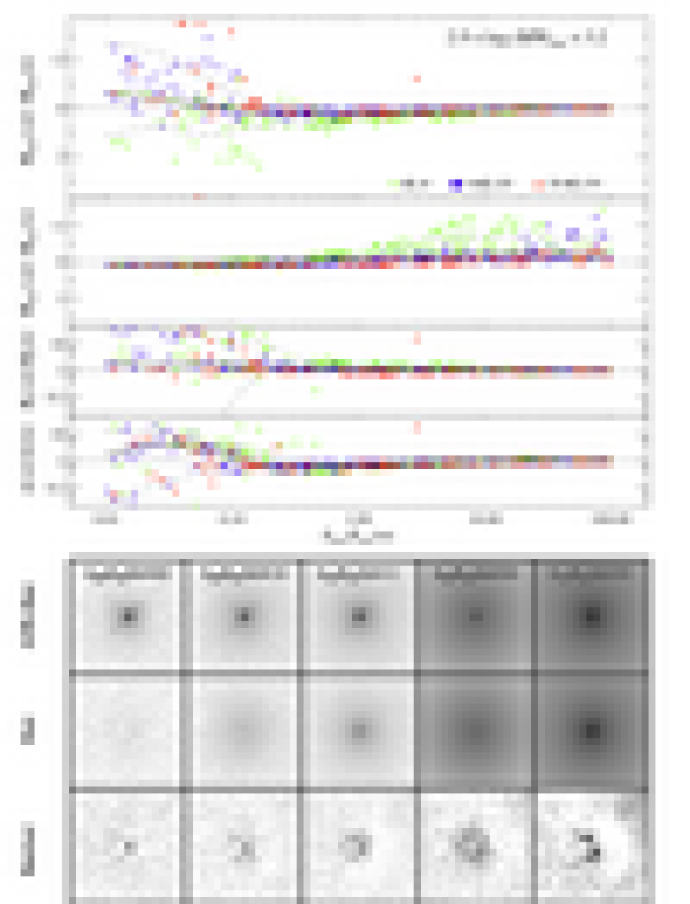
Figure 18d: Simulation results for $10^{2.8}\leq$ $(S/N)_{\rm nuc}$ $\leq 10^{3.2}$.

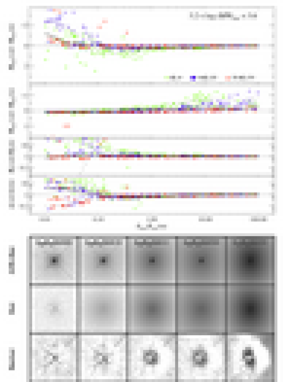
Figure 18e: Simulation results for $10^{3.2}\leq$ $(S/N)_{\rm nuc}$ $\leq 10^{3.6}$.

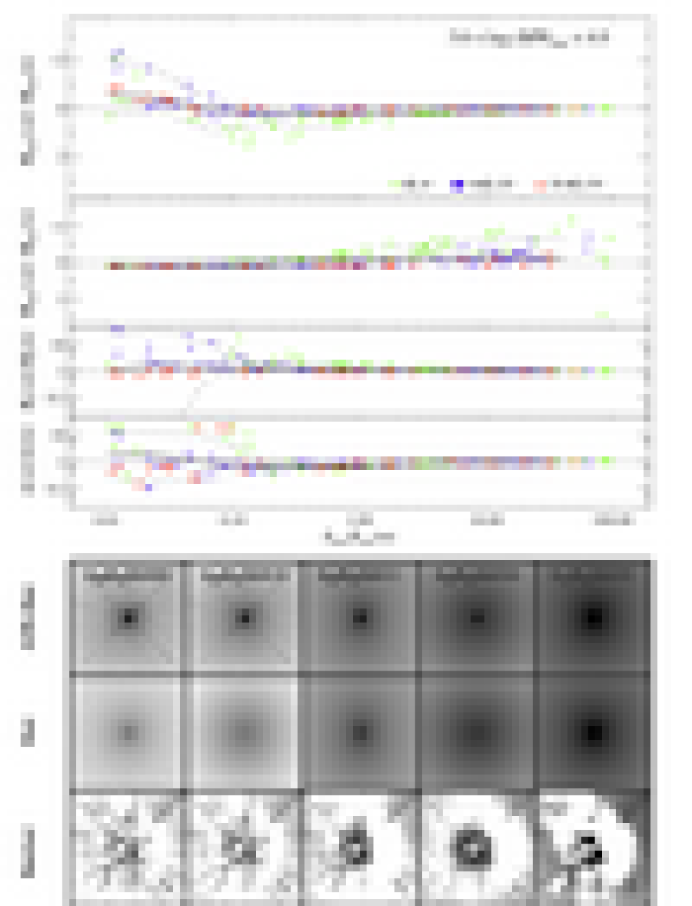
Figure 18f: Simulation results for $10^{3.6}\leq$ $(S/N)_{\rm nuc}$ $\leq 10^{4.0}$.

References

- (1) Bahcall, J. N., Kirhakos, S., Saxe, D. H., & Schneider, D. P. 1997, ApJ, 479, 642
- (2) Barth, A. J., Greene, J. E., & Ho, L. C. 2005, ApJ, 619, L151
- (3) Boyce, P. J., et al. 1998, MNRAS, 298, 121
- (4) Byun, Y. I., & Freeman, K. C. 1995, ApJ, 448, 563
- (5) de Jong, R. S. 1996, A&AS, 118, 557
- (6) de Souza, R. E., Gadotti, D. A., & dos Anjos, S. 2004, ApJS, 153, 411
- (7) Dunlop, J. S., McLure, R. J., Kukula, M. J., Baum, S. A., O’Dea, C. P., & Hughes, D. H. 2003, MNRAS, 340, 1095
- (8) Ferrarese, L., & Merritt, D. 2000, ApJ, 539, L9
- (9) Floyd, D. J. E., Kukula, M. J., Dunlop, J. S., McLure, R. J., Miller, L., Percival, W. J., Baum, S. A., & O’Dea, C. P. 2004, MNRAS, 355, 196
- (10) Gebhardt, K., et al. 2000, ApJ, 539, L13
- (11) Graham, A. W., & Driver, S. P. 2007, ApJ, 655, 77
- (12) Greene, J. E., & Ho, L. C. 2005a, ApJ, 627, 721
- (13) ——. 2005b, ApJ, 630, 122
- (14) ——. 2006, ApJ, 641, 117
- (15) Greene, J. E., Ho, L. C., & Barth, A. J. 2008, ApJ, in press
- (16) Griffiths, R. E., et al. 1994, ApJ, 437, 67
- (17) Häring, N., & Rix, H.-W. 2004, ApJ, 604, L89
- (18) Ho, L. C. 1999, in Observational Evidence for Black Holes in the Universe, ed. S. K. Chakrabarti (Dordrecht: Kluwer), 157
- (19) ——. 2004, ed., Carnegie Observatories Astrophysics Series, Vol. 1: Coevolution of Black Holes and Galaxies (Cambridge: Cambridge Univ. Press)
- (20) ——. 2007, ApJ, 669, 821
- (21) Ho, L. C., Darling, J., & Greene, J. E. 2008, ApJ, in press (arXiv:0803.1952)
- (22) Hutchings, J. B., Frenette, D., Hanisch, R., Mo, J., Dumont, P. J., Redding, D. C., & Neff, S. G. 2002, AJ, 123, 2936
- (23) Jahnke, K., et al. 2004, ApJ, 614, 568
- (24) Kaspi, S., Smith, P. S., Netzer, H., Maoz, D., Jannuzi, B. T., & Giveon, U. 2000, ApJ, 533, 631
- (25) Kim, M., Ho, L. C., Peng, C. Y., Barth, A. J., Im, M., Martini, P., & Nelson, C. H. 2008, ApJ, in press
- (26) Kim, M., Ho, L. C., Peng, C. Y., & Im, M. 2007, ApJ, 658, 107
- (27) Kormendy, J., & Gebhardt, K. 2001, in 20th Texas Symposium on Relativistic Astrophysics, ed. H. Martel & J. C. Wheeler (Melville: AIP), 363
- (28) Kormendy, J., & Kennicutt, R. C. 2004, ARA&A, 42, 603
- (29) Kormendy, J., & Richstone, D. O. 1995, ARA&A, 33, 581
- (30) Krist, J. 1995, in Astronomical Data Analysis Software and Systems IV, ed. R. A. Shaw, H. E. Payne, & J. J. E. Hayes (San Francisco: ASP), 349
- (31) Magorrian, J., et al. 1998, AJ, 115, 2285
- (32) Marconi, A., & Hunt, L. K. 2003, ApJ, 589, L21
- (33) McLure, R. J., & Dunlop, J. S. 2002, MNRAS, 331, 795
- (34) McLure, R. J., Kukula, M. J., Dunlop, J. S., Baum, S. A., O’Dea, C. P., & Hughes, D. H. 1999, MNRAS, 308, 377
- (35) Nelson, C. H., Green, R. F., Bower, G., Gebhardt, K., & Weistrop, D. 2004, ApJ, 615, 652
- (36) Onken, C. A., Ferrarese, L., Merritt, D., Peterson, B. M., Pogge, R. W., Vestergaard, M., & Wandel, A. 2004, ApJ, 615, 645
- (37) Peng, C. Y., Ho, L. C., Impey, C. D., & Rix, H.-W. 2002, AJ, 124, 266
- (38) Peng, C. Y., Impey, C. D., Ho, L. C., Barton, E. J., & Rix, H.-W. 2006a, ApJ, 640, 114
- (39) Peng, C. Y., Impey, C. D., Rix, H.-W., Kochanek, C. S., Keeton, C. R., Falco, E. E., Lehár, J., & McLeod, B. A. 2006b, ApJ, 649, 616
- (40) Peterson, B. M. 2007, in The Central Engine of Active Galactic Nuclei, ed. L. C. Ho & J.-M. Wang (San Francisco: ASP), 3
- (41) Salviander, S., Shields, G. A., Gebhardt, K., & Bonning, E. W. 2007, ApJ, 662, 131
- (42) Sánchez, S. F., et al. 2004, ApJ, 614, 586
- (43) Sérsic, J. L. 1968, Atlas de Galaxias Australes (Córdoba: Obs. Astron., Univ. Nac. Córdoba)
- (44) Schade, D. J., Boyle, B. J., & Letawsky, M. 2000, MNRAS, 315, 498
- (45) Shen, J., Vanden Berk, D. E., Schneider, D. P., & Hall, P. B. 2008, AJ, 135, 928
- (46) Simard, L., et al. 2002, ApJS, 142, 1
- (47) Sirianni, M., et al. 2005, PASP, 117, 1049
- (48) Wadadekar, Y., Robbason, B., & Kembhavi, A. 1999, AJ, 117, 1219
- (49) Wandel, A., Peterson, B. M., & Malkan, M. A. 1999, ApJ, 526, 579
- (50) Woo, J.-H., Treu, T., Malkan, M. A., & Blandford, R. D. 2006, ApJ, 645, 900