Compressibility of solid helium

Abstract

The compressibility of solid helium (³He and ⁴He) in the hcp and fcc phases has been studied by path-integral Monte Carlo. Simulations were carried out in both canonical ($NVT$) and isothermal-isobaric ($NPT$) ensembles at temperatures between 10 and 300 K, showing consistent results in both ensembles. For pressures between 4 and 10 GPa, the bulk modulus $B$ is found to decrease by about 10%, when temperature increases from the low-temperature limit to the melting temperature. The isotopic effect on the bulk modulus of helium crystals has been quantified in a wide range of parameters. At 25 K and pressures on the order of 1 GPa, the relative difference between ³He and ⁴He amounts to about 2%. The thermal expansion has been also quantified from results obtained in both $NPT$ and $NVT$ simulations.

I Introduction

In the last decades there has been a continuous progress in the study of different types of substances under extreme conditions of pressure and temperature, thus enlarging appreciably the experimentally accessible region of phase diagrams Young (1991). In particular, the influence of controlled hydrostatic pressure on structural, thermodynamic, and electronic properties of various kinds of solids has been deeply studied. Pressures on the order of tens of GPa can now be routinely applied to real materials Loubeyre et al. (1993); Hemley et al. (1989); Shimizu et al. (2001); Errandonea et al. (2006).

Solid helium, in spite of having been studied for many years, has a broad interest in condensed matter physics because of its peculiar character of “quantum solid”. In particular, its zero-point vibrational energy and associated anharmonic effects are markedly larger than in most known solids Glyde (1976). In addition, its electronic simplicity allows one to carry out detailed studies, that would be enormously difficult for other materials Ceperley (1995); Nabi et al. (2005); Cazorla and Boronat (2008). The interest on the behavior of solids under high pressures has been also focused on solid helium. Thus, diamond-anvil-cell and shock-wave experiments have allowed to study the equation of state (EOS) of solid ⁴He up to pressures on the order of 50 GPa Polian and Grimsditch (1986); Mao et al. (1988); Loubeyre et al. (1993). In last years, the effect of pressure on heavier rare-gas solids has also been of interest for both experimentalists Shimizu et al. (2001); Errandonea et al. (2002) and theorists Neumann and Zoppi (2000); Iitaka and Ebisuzaki (2001); Dewhurst et al. (2002); Tsuchiya and Kawamura (2002).

The Feynman path-integral formulation of statistical mechanics Feynman (1972); Kleinert (1990) is well suited to study thermodynamic properties of solids at temperatures lower than their Debye temperature $\Theta_{D}$, where the quantum character of the atomic nuclei becomes important. In particular, the combination of path integrals with computer simulation methods, such as Monte Carlo or molecular dynamics, has revealed as a powerful technique to carry out quantitative and nonperturbative studies of many-body quantum systems at finite temperatures. This has allowed to study several properties of solids further than the usual harmonic or quasiharmonic approximations Ceperley (1995).

The path-integral Monte Carlo (PIMC) method has been used to study several properties of solid helium Ceperley (1995); Ceperley et al. (1996); Barrat et al. (1989); Boninsegni et al. (1994); Chang and Boninsegni (2001); Herrero (2006, 2007), as well as heavier rare-gas solids Cuccoli et al. (1993); Müser et al. (1995); Chakravarty (2002); Neumann and Zoppi (2002); Herrero (2002); Herrero and Ramírez (2005). For helium, in particular, this method has predicted kinetic-energy values Ceperley et al. (1996) and Debye-Waller factors Draeger and Ceperley (2000) in good agreement with data derived from experiments Arms et al. (2003); Venkataraman and Simmons (2003). PIMC simulations have been also employed to study the isotopic shift in the helium melting curve Barrat et al. (1989); Boninsegni et al. (1994). The EOS of solid helium at $T$ = 0 has been studied by diffusion Monte Carlo in a wide density range Moroni et al. (2000); Cazorla and Boronat (2008), as well as at finite temperatures by using PIMC simulations with several interatomic potentials Chang and Boninsegni (2001).

In last years, there has been a debate on the existence of supersolidity in ⁴He at temperatures lower than 1 K Kim and Chan (2004); Rittner and Reppy (2007); Clark et al. (2007); Ceperley and Bernu (2004). This debate is still open, but is out of the scope of this paper, since we consider here solid helium at temperatures higher than 10 K, where quantum exchange effects between atomic nuclei are not relevant.

In this paper, we study the compressibility of solid ³He and ⁴He by PIMC simulations. We employ the isothermal-isobaric ($NPT$) ensemble, which allows us to consider properties of these solids along well-defined isobars. For comparison, we present also results of PIMC simulations in the canonical ($NVT$) ensemble. By comparing results for ³He and ⁴He, we analyse isotopic effects on the compressibility as a function of pressure.

The paper is organized as follows. In Sec. II, the computational method is described. In Sec. III we present and discuss the results, that are given in several subsections dealing with thermodynamic consistency, pressure and temperature dependence of the bulk modulus, isotopic effects, and thermal expansion. Finally, in Sec. IV we present the conclusions.

II Method

Equilibrium properties of solid ³He and ⁴He in the face-centred cubic (fcc) and hexagonal close-packed (hcp) phases have been calculated by PIMC simulations. The PIMC method relies on an isomorphism between the quantum system under consideration and a fictitious classical one, obtained by replacing each quantum particle by a cyclic chain of $Q$ classical particles ($Q$: Trotter number), connected by harmonic springs with a temperature-dependent force constant. This isomorphism appears as a consequence of discretizing the density matrix along cyclic paths, which is usual in the path-integral formulation of statistical mechanics Feynman (1972); Kleinert (1990). Details on this computational method are given elsewhere Chandler and Wolynes (1981); Gillan (1988); Ceperley (1995); Noya et al. (1996).

Helium atoms were considered as quantum particles interacting through an effective interatomic potential, composed of a two-body and a three-body part. For the two-body interaction, we employed the potential developed by Aziz et al. Aziz et al. (1995) (the so-called HFD-B3-FCI1 potential). For the three-body part we took a Bruch-McGee-type potential Bruch and McGee (1973); Loubeyre (1987), with the parameters given by Loubeyre Loubeyre (1987), but with parameter $A$ in the attractive exchange interaction rescaled by a factor 2/3, as suggested in Ref. Boninsegni et al. (1994). This interatomic potential was found earlier to describe well the vibrational energy and equation-of-state of solid helium in a broad range of pressures and temperatures Herrero (2006).

Our simulations were based on the so-called “primitive” form of PIMC Chandler and Wolynes (1981); Singer and Smith (1988). We considered explicitly two- and three-body terms in the simulations. The actual consideration of three-body terms did not allow us to use effective forms for the density matrix, developed to simplify the calculation when only two-body terms are explicitly considered Boninsegni et al. (1994). Quantum exchange effects between atomic nuclei were not taken into account, because they are negligible for solid helium at the temperatures and pressures studied here. (This is expected to be valid assuming the absence of vacancies and for temperatures higher than the exchange frequency $\sim 10^{-6}$ K Ceperley (1995).) To calculate the energy we have used the “crude” estimator, as defined in Refs. Chandler and Wolynes (1981); Singer and Smith (1988).

We have employed both the canonical ($NVT$) ensemble and the isothermal-isobaric ($NPT$) ensemble. Our simulations were performed on supercells of the fcc and hcp unit cells, including 500 and 432 helium atoms respectively. To check the convergence of our results with system size, we carried out some simulations for other supercell sizes, and found that finite-size effects for $N>400$ atoms are negligible for the quantities studied here. In particular, changes of the bulk modulus with the size of the simulation cell were found to be smaller than the statistical error bar of the values derived from our simulations.

Sampling of the configuration space was carried out by the Metropolis method at temperatures between 12 K and the melting temperature at each considered pressure. For given temperature and pressure, a typical run consisted of $10^{4}$ Monte Carlo steps for system equilibration, followed by $4\times 10^{5}$ steps for the calculation of ensemble average properties. Each step included attempts to move every replica of every atom in the simulation cell. In the $NPT$ simulations, it also included an attempt to change the volume. To keep roughly constant the accuracy of the computed quantities at different temperatures, we took a Trotter number $Q$ proportional to the inverse temperature, so that $QT$ = 3000 K. This means that for solid helium at $T$ = 20 K we had $Q$ = 150, and a PIMC simulation for $N=500$ atoms effectively includes 75000 “classical” particles. More technical details are given in Refs. Noya et al. (1997); Herrero (2002, 2006).

In the $NVT$ ensemble the pressure and isothermal bulk modulus $B=-V({\partial P}/{\partial V})_{T}$ can be obtained from thermal averages of various quantities obtained in PIMC simulations, as shown in Appendix A. The derivation is straightforward from the partition function $Z_{NVT}$ for $N$ quantum particles in the canonical ensemble, but is rather tedious in the case of the bulk modulus, due to the number of terms appearing in the volume derivatives. In particular, $B$ can be obtained from Eqs. (16) and (A.2) in Appendix A. In the $NPT$ ensemble, the isothermal bulk modulus is related to the mean-square fluctuations of the volume $V$ of the simulation cell by the expression:

$$\sigma_{V}^{2}=\frac{V}{B}k_{B}T\;,$$ (1)

as shown in Appendix B.

III Results and discussion

III.1 Consistency checks

We have calculated the bulk modulus in the $NPT$ and $NVT$ ensembles. In general, we prefer the isothermal-isobaric ensemble, so that we can study solids along well-defined isotherms. $NVT$ simulations are, however, frequently used in PIMC simulations Ceperley (1995); Ceperley et al. (1996); Draeger and Ceperley (2000), and a comparison of results obtained in both ensembles seems necessary as a consistency check of the method, and in particular for the case of solid helium.

We discuss first results obtained in the $NPT$ ensemble. At constant pressure, the relative fluctuations in the volume, $\sigma_{V}/V$, can be found from Eq. (1):

$$\frac{\sigma_{V}}{V}=\left(\frac{k_{B}T}{BV}\right)^{\frac{1}{2}}\;.$$ (2)

For hcp ⁴He at 25 K we found in PIMC simulations $\sigma_{V}/V=2.9\times 10^{-3}$ for $P$ = 2 GPa, and a lower value of $1.4\times 10^{-3}$ for 20 GPa (for a simulation cell including $N$ = 432 atoms). This means that the product $BV$ increases as the pressure is raised [see Eq. (2], in spite of the reduction of $V$, indicating that the growth of bulk modulus with the pressure dominates in the product $BV$ (see below).

For a cubic crystal, the fluctuations in the lattice parameter $a$ can be derived from Eq. (1) to give:

$$\sigma_{a}^{2}=\frac{k_{B}T}{9L^{3}aB}\;,$$ (3)

where $L^{3}$ is the number of cubic unit cells in a simulation cell with side length $La$. From Eq. (3) one can see that the relative fluctuation in the lattice parameter, $\sigma_{a}/a$, scales as $L^{-3/2}$. This normalized fluctuation for fcc ⁴He is displayed in Fig. 1 as a function of $L^{-3/2}$. Shown are results of PIMC simulations in the $NPT$ ensemble at $T$ = 100 K and two pressures: 2 and 7 GPa. The linear dependence shown in this figure agrees with the dependence of $\sigma_{a}$ on the simulation-cell size given by Eq. (3). The different slopes of these lines are basically due to the change of compressibility with pressure.

Figure 1: Relative fluctuation of the lattice parameter, $\sigma_{a}/a$, of fcc ⁴He vs $L^{-3/2}$, for simulation cells of lateral size $La$. Shown are results of PIMC simulations for two pressures (2 and 7 GPa) at $T$ = 100 K, and for $L$ = 3, 4, 5, and 7. Error bars are less than the symbol size.

To check the thermodynamic consistency of our simulations in both $NPT$ and $NVT$ ensembles we have carried out several tests. The first obvious test consists in taking the crystal volume derived from isothermal-isobaric simulations, and using it as an input in $NVT$ simulations at the same temperature. The latter should give the same pressure [using Eq. (12)] as that used earlier in the $NPT$ simulations. As an example, for fcc ⁴He at 25 K and 1 GPa, we find first a lattice parameter $a$ = 3.6955 Å, that introduced as an input in $NVT$ simulations yields a pressure of 1.0002(5) GPa, in good agreement with the input in the previous $NPT$ simulations. Going on with the same set of parameters, we can also check the consistency of the bulk modulus $B$ derived from both types of simulations. At constant pressure ($P$ = 1 GPa), we find $B_{NPT}$ = 4.50(2) GPa from the volume fluctuations [see Eq. (22) in Appendix B] vs $B_{NVT}$ = 4.47(2) GPa derived at constant volume by using expressions (16) and (A.2).

III.2 Pressure and temperature dependence

We now consider the pressure dependence of the bulk modulus, as derived from our PIMC simulations. This is shown in Fig. 2 for ⁴He at three temperatures. In this figure, $T$ decreases from top to bottom: $T$ = 25, 150, and 300 K; open and filled symbols correspond to hcp and fcc helium, respectively. At each considered temperature, we present data for the pressure region where the solid was stable (or metastable) along the PIMC simulations, a region that becomes broader as the temperature is lowered. In addition to the typical rise of $B$ for increasing pressure, we find that for a given pressure, $B$ decreases as the temperature is raised. In the pressure range shown in Fig. 2 one also observes a departure of linearity in the dependence of $B$ on pressure. By fitting these results to the expression $B=B_{0}+B_{0}^{\prime}P+\frac{1}{2}B_{0}^{\prime\prime}P^{2}$, we can find the pressure derivatives at $P=0$ ($B_{0}^{\prime}$ and $B_{0}^{\prime\prime}$). Thus, for $T$ = 25 K we obtain $B_{0}$ = 0.47 GPa, $B_{0}^{\prime}$ = 4.01, and $B_{0}^{\prime\prime}$ = –0.068 GPa^-1.

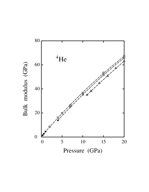
Figure 2: Isothermal bulk modulus of solid ⁴He as a function of pressure at three temperatures: 25 K (squares), 150 K (circles), and 300 K (triangles). Open and filled symbols correspond to hcp and fcc helium, respectively. Error bars are smaller than the symbol size. Dashed lines are fits to the data points using the expression: $B=B_{0}+B_{0}^{\prime}P+\frac{1}{2}B_{0}^{\prime\prime}P^{2}$.

For the other temperatures shown in Fig. 2 ($T$ = 150 and 300 K), an extrapolation of the results to $P=0$ yields negative values of $B_{0}$, indicating that the solid is mechanically unstable at these temperatures for low pressures. At 25 K and zero pressure, even though the liquid is known to be the stable phase, the solid can still be metastable, as it has not yet reached the limit of mechanical stability, or the spinodal line . Apart from this, the curves $B(P)$ at the considered temperatures are rather parallel one to the other in the common stability region.

It is interesting to compare the bulk modulus obtained here for solid helium with those of heavier rare-gas solids at the same conditions. For example, at $T$ = 20 K and $P$ = 1 GPa, we find for solid ⁴He: $B$ = 4.53 GPa, vs 7.20 and 9.43 for Ne and Ar, respectively Herrero and Ramírez (2005). This is in line with the known result that the bulk modulus increases with atomic mass for given values of temperature and pressure Herrero and Ramírez (2005).

Rare-gas solids have been studied in metastable conditions, even at negative pressures Herrero (2003). They have been found to be metastable in PIMC simulations close to the spinodal point, defined as the point at which the compressibility $\kappa=1/B$ diverges (or the bulk modulus vanishes). Thus, for solid Ne and Ar at 5 K, the spinodal point was found at $P=-91$ and $-245$ MPa. For solid helium, we could not approach the spinodal point at any temperature, due to the large quantum fluctuations that make the solid to be unstable along the simulations. This happened even at zero pressure and relatively low temperature, in spite of the fact that the expected bulk modulus at these conditions is still far from vanishing. For example, at 25 K we find for solid helium $B_{0}$ = 0.47 GPa, as derived from extrapolation of the results obtained at $P>$ 0.2 GPa (see above and Fig. 2), but the solid was unstable in our simulations at $P<$ 0.2 GPa.

Figure 3: Isothermal bulk modulus of solid ⁴He as a function of temperature at three hydrostatic pressures: 4 GPa (squares), 7 GPa (circles), and 10 GPa (triangles). Open and filled symbols correspond to hcp and fcc helium, respectively. Error bars of the simulation results are on the order of the symbol size. Dashed lines are guides to the eye.

The temperature dependence of the bulk modulus is displayed in Fig. 3 for three different pressures. Here again open and filled symbols indicate hcp and fcc helium, respectively. For each pressure under consideration, the plotted data correspond to the temperature region where we found the solids to be (meta)stable along the PIMC simulations. For each pressure, the bulk modulus decreases as the temperature is raised, and this decrease is similar for the different pressures. In fact, the obtained curves $B(T)$ are parallel within the statistical error of our simulations. In the whole accessible temperature range, the bulk modulus decreases by 2.1, 2.6, and 3.1 GPa, for $P$ = 4, 7, and 10 GPa, respectively. These values amount to 13.0, 9.8, and 8.5 % of the corresponding bulk modulus at 25 K.

Figure 4: Isothermal bulk modulus of solid ⁴He versus density. Open squares represent results of path-integral Monte Carlo simulations in the $NPT$ ensemble. Error bars are less than the symbol size. A solid line indicates the bulk modulus derived by Zha et al. Zha et al. (2004) from Brillouin scattering experiments. The dashed line is a guide to the eye.

To connect with data derived from experiment, we note that Zha et al. Zha et al. (2004) have obtained the bulk modulus of solid ⁴He from Brillouin scattering measurements. From these results, they derived the dependence of the isothermal bulk modulus upon material density at 300 K. In Fig. 4 we present results of our PIMC simulations for ⁴He at 300 K (open squares) along with those derived from Brillouin scattering experiments at room temperature (solid line). At this temperature, the density region between 0.95 and 1.25 g cm^-3 corresponds to a pressure between 12 and 29 GPa. At $\rho<1\text{ g cm}^{-3}$, our results coincide within error bars with those derived from Brillouin scattering, and at higher densities the bulk modulus derived from PIMC simulations is somewhat larger. For example, at density $\rho$ = 1 and 1.25 g/cm³, Zha et al. Zha et al. (2004) obtained $B$ = 42.1 and 79.9 GPa respectively, to be compared with $B$ = 44 and 86 GPa yielded by our PIMC simulations of ⁴He at the same densities and $T$ = 300 K. This means that at $\rho=1.25$ g cm^-3, the difference amounts to about 7%.

III.3 Isotopic effect

An interesting point in this context is the influence of the atomic mass on the solid compressibility. This isotopic effect can be readily obtained from PIMC simulations, since the mass is an input parameter in these calculations. Similar isotopic effects have been studied earlier for the melting curve Barrat et al. (1989); Boninsegni et al. (1994) and molar volume Herrero (2006, 2007) of solid helium. For a given material, lighter isotopes form more compressible solids, as a consequence of an increase in the molar volume. This is in fact due to a combination of the anharmonicity in the interatomic potential and zero-point vibrations, which are most important at low temperature. Since these quantum vibrations are especially large in the case of helium, due to its low mass, the isotopic effect on the bulk modulus is expected to be appreciable.

Thus, one expects the bulk modulus of solid ⁴He to be larger than that of ³He. This is in fact the case, as derived from our PIMC simulations. In Fig. 5 we display the difference $\Delta B=B_{4}-B_{3}$ as a function of pressure at $T$ = 25 K. For example, at 1 GPa and 25 K we find $B=4.40$ and $4.50\pm 0.01$ GPa for ³He and ⁴He, respectively, and the difference between both isotopes amounts to 2.2%. At the same temperature and 7 GPa, we obtained $B$ = 26.20 and 26.59 GPa, which translates to a relative difference of 1.5%. This relative change in bulk modulus associated to the isotopic mass is appreciable, and slightly larger than that found for the isotopic effect on the molar volume of helium crystals. Thus, at a pressure of 1 and 7 GPa and $T$ = 25 K, we find a volume difference of 1.8 and 0.9%, when comparing ³He and ⁴He Herrero (2007). In general, given a temperature, the relative changes in volume and compressibility decrease for increasing pressure, since the solid behaves as if it was “more classical” Etters and Danilowicz (1974); Herrero and Ramírez (2005), and isotopic effects (of quantum origin) are consequently reduced.

Figure 5: Isotopic effect on the isothermal bulk modulus as a function of pressure. Shown is the difference $\Delta B=B_{4}-B_{3}$ between the bulk modulus of ⁴He and ³He at 25 K. Filled and open symbols represent data for fcc and hcp helium, respectively.

III.4 Thermal expansion

At this point, it is worthwhile comparing the temperature dependence of the bulk modulus obtained at fixed volume and fixed pressure, from PIMC simulations in the $NVT$ and $NPT$ ensembles, respectively. In Fig. 6 we have plotted our results for $B$, as derived in both cases. On one side, the simulations in the isothermal-isobaric ensemble were carried out at a pressure $P$ = 1 GPa, and the results obtained are represented in Fig. 6 as circles. On the other side, simulations in the canonical ensemble (at various temperatures) were performed for the volume obtained in $NPT$ simulations at $T$ = 25 K and $P$ = 1 GPa. Results of these $NVT$ simulations are displayed as open squares. As expected, $B$ obtained in both types of simulations agree with each other (within error bars) at $T\leq$ 25 K. At higher temperatures, the $NPT$ simulations yield values of the bulk modulus smaller than those derived from $NVT$ simulations. This is due to the thermal expansion, that is taken into account in the simulations at constant pressure, but is neglected in the constant-volume simulations. In general, an increase in crystal volume causes a decrease in the bulk modulus.

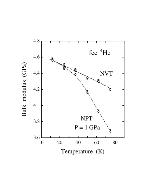
Figure 6: Bulk modulus vs temperature, as derived from PIMC simulations at constant volume (squares) and constant pressure (circles). The simulations in the $NVT$ ensemble were carried out with the volume obtained at $P$ = 1 GPa and $T$ = 25 K. Lines are guides to the eye.

In this context, another application of our PIMC simulations consists in the calculation of the thermal expansion coefficient

$$\alpha=\frac{1}{V}\left(\frac{\partial V}{\partial T}\right)_{P}\,,$$ (4)

which can be obtained in the canonical ensemble by using the expression Callen (1960):

$$\alpha=\frac{1}{B}\left(\frac{\partial P}{\partial T}\right)_{V}\;.$$ (5)

This equation in fact relates the thermal expansion with the compressibility through the temperature derivative of the pressure at constant volume. In connection with Eq. (5), we note that the pressure obtained in $NVT$ simulations (with a fixed lattice parameter $a$ = 3.6955 Å) increases from 1 GPa to 1.3 GPa when temperature rises from 25 to 75 K. At 25 K, we have $B$ = 4.46 GPa and $({\partial P}/{\partial T})_{V}=8.87\times 10^{-4}$ GPa K^-1, giving $\alpha_{NVT}=1.99\times 10^{-4}$ K^-1. This result is in agreement with that found directly from the volume change obtained in the $NPT$ simulations, which yields $\alpha_{NPT}=2.03\times 10^{-4}\text{K}^{-1}$.

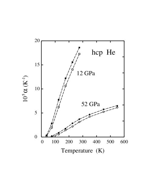
Figure 7: Temperature dependence of the thermal expansion coefficient $\alpha$ of hcp helium, as derived from PIMC simulations at $P=$ 12 GPa and 52 GPa. Open and filled symbols correspond to ³He and ⁴He, respectively. Error bars are on the order of the symbol size. Dashed lines are guides to the eye.

Finally, in Fig. 7 we present results of the thermal expansion coefficient $\alpha$ yielded by our simulations in the isothermal-isobaric ensemble at two (high) pressures. We give values for both ³He and ⁴He in the hcp phase. First, we observe an important decrease in $\alpha$ as the pressure is raised. For ⁴He at 300 K, we find a reduction in $\alpha$ by a factor of five, when increasing $P$ from 12 to 52 GPa. Second, we note that the thermal expansion is smaller for ³He than for ⁴He. This is easy to understand, since the molar volume of solid ³He is larger than that of ⁴He Herrero (2006), and both volumes have to converge one to the other in the high-temperature (classical) limit.

IV Conclusions

Path-integral Monte Carlo simulations in both $NVT$ and $NPT$ ensembles have been shown to be well suited to analyse the temperature and pressure dependence of the bulk modulus of solid helium. In the isothermal-isobaric ensemble, $B$ can be derived from the volume fluctuations along a simulation run. In the canonical ensemble, a calculation of $B$ is more elaborate, but can be carried out from thermal averages of various intermediate quantities obtained in PIMC simulations. Both ensembles $NVT$ and $NPT$ give consistent results for the compressibility and thermal expansion of ³He and ⁴He in the whole region of temperatures and pressures considered here.

At a given pressure, the bulk modulus decreases as temperature rises. For pressures between 4 and 10 GPa, the change in $B$ has been found to be on the order of 10%, when temperature increases from the low-$T$ limit to the melting temperature of the material.

Solid ³He is more compressible than ⁴He. At a given $T$, the difference between bulk modulus of both solids increases as pressure rises, but the relative difference between them decreases. This isotopic effect on the compressibility of solid helium is appreciable in the range of temperatures and pressures studied here. In fact, at 25 K and pressures on the order of 1 GPa, it amounts to about 2%.

Apart from a precise calculation of the bulk modulus, PIMC simulations in the canonical ensemble can be also used to study accurately the thermal expansion of the solids under consideration at a given pressure.

Appendix A Pressure and bulk modulus in the $NVT$ ensemble

A.1 Pressure

In the path-integral formalism, the canonical partition function for $N$ identical quantum particles obeying Boltzmann statistics (no particle exchange) can be written as Chandler and Wolynes (1981); Gillan (1988):

$$Z_{NVT}=K\int\prod_{i=1}^{N}\prod_{j=1}^{Q}d{\bf r}_{ij}\exp\left(-\beta\sum_{j=1}^{Q}\left[C\sum_{i=1}^{N}({\bf r}_{i,j+1}-{\bf r}_{ij})^{2}+\frac{1}{Q}\,\Phi({\bf r}_{1j},...,{\bf r}_{Nj})\right]\right),$$ (6)

where ${\bf r}_{ij}$ ($i=1,...,N;j=1,...,Q$) are Cartesian coordinates of the $N$ particles at imaginary time $j$, $\beta=(k_{B}T)^{-1}$, and $\Phi({\bf r}_{1j},...,{\bf r}_{Nj})$ is the potential energy. We have defined

$$K=\frac{1}{N!}\left(\frac{mQ}{2\pi\beta\hbar^{2}}\right)^{3NQ/2}$$ (7)

and

$$C=\frac{mQ}{2\beta^{2}\hbar^{2}}\;.$$ (8)

The coordinates are subject to the cyclic condition ${\bf r}_{i,Q+1}={\bf r}_{i1}$ for all particles $i=1,...,N$. Changing ${\bf r}_{ij}$ to reduced coordinates ${\bf s}_{ij}=V^{-1/3}{\bf r}_{ij}$, we find:

$$Z_{NVT}=KV^{NQ}\int\prod_{i=1}^{N}\prod_{j=1}^{Q}d{\bf s}_{ij}\exp\left[-\beta H(\beta,V,\{{\bf s}_{ij}\})\right]\;,$$ (9)

where we have defined

$$H(\beta,V,\{{\bf s}_{ij}\})=CV^{2/3}\sum_{i=1}^{N}\sum_{j=1}^{Q}({\bf s}_{i,j+1}-{\bf s}_{ij})^{2}+$$

$$+\frac{1}{Q}\,\sum_{j=1}^{Q}\Phi(V^{1/3}{\bf s}_{1j},...,V^{1/3}{\bf s}_{Nj})$$ (10)

and the dependence of $H$ on $\beta$, $V$, and the coordinates ${\bf s}_{ij}$ has been explicitly indicated.

The pressure is given by

$$P=\frac{1}{\beta}\frac{1}{Z_{NVT}}\frac{\partial Z_{NVT}}{\partial V},$$ (11)

and from the volume derivative of $Z_{NVT}$ one finds:

$$P=\frac{NQ}{\beta V}-\frac{2}{3V}\langle E_{h}\rangle-\left<\Phi_{V}\right>$$ (12)

where $E_{h}$ refers to the “harmonic” energy:

$$E_{h}=C\sum_{i=1}^{N}\sum_{j=1}^{Q}({\bf r}_{i,j+1}-{\bf r}_{ij})^{2}=CV^{2/3}\sum_{i=1}^{N}\sum_{j=1}^{Q}({\bf s}_{i,j+1}-{\bf s}_{ij})^{2}$$ (13)

and

$$\Phi_{V}=\frac{1}{Q}\sum_{j=1}^{Q}\frac{\partial\Phi(V^{1/3}{\bf s}_{1j},...,V^{1/3}{\bf s}_{Nj})}{\partial V}\;.$$ (14)

A.2 Bulk modulus

The isothermal bulk modulus is:

$$B=-V\left(\frac{\partial P}{\partial V}\right)_{T}$$ (15)

and substituting Eq. (11) for the pressure, we have:

$$B=V\beta P^{2}-\frac{V}{\beta Z_{NVT}}\frac{\partial^{2}Z_{NVT}}{\partial V^{2}}\;.$$ (16)

Taking a second volume derivative of $Z_{NVT}$, we find:

$$\frac{1}{\beta Z_{NVT}}\frac{\partial^{2}Z_{NVT}}{\partial V^{2}} = \frac{NQ(NQ-1)}{\beta V^{2}}+\frac{1}{3V^{2}}\left(\frac{2}{3}-4NQ\right)\left<E_{h}\right>-\frac{2NQ}{V}\left<\Phi_{V}\right>+\frac{4}{9}\frac{\beta}{V^{2}}\left<E_{h}^{2}\right>+$$

$$+ \frac{4}{3}\frac{\beta}{V}\left<E_{h}\Phi_{V}\right>-\frac{1}{Q}\left<\frac{\partial\Phi_{V}}{\partial V}\right>+\beta\left<\Phi_{V}^{2}\right>$$

Finally, Eqs. (16) and (A.2) give us the bulk modulus $B$ at volume $V$ and temperature $T$.

Appendix B Compressibility in the $NPT$ ensemble

We now have the partition function

$$Z_{NPT}=\int_{0}^{\infty}dV{\rm e}^{-\beta PV}Z_{NVT}\;.$$ (18)

To obtain the compressibility, we calculate the pressure derivatives of $\ln Z_{NPT}$. We find:

$$\frac{\partial\ln Z_{NPT}}{\partial P}=\frac{1}{Z_{NPT}}\frac{\partial Z_{NPT}}{\partial P}=-\beta\left<V\right>$$ (19)

and

$$\frac{\partial^{2}\ln Z_{NPT}}{\partial P^{2}} = -\frac{1}{Z_{NPT}^{2}}\left(\frac{\partial Z_{NPT}}{\partial P}\right)^{2}+\frac{1}{Z_{NPT}}\frac{\partial^{2}Z_{NPT}}{\partial P^{2}}=$$ (20)

$$= -\beta^{2}\left<V\right>^{2}+\beta^{2}\langle V^{2}\rangle=-\beta^{2}\sigma_{V}^{2}\;,$$

where $\sigma_{V}^{2}$ is the mean square fluctuation of the volume. Moreover, from Eq. (19):

$$\frac{\partial^{2}\ln Z_{NPT}}{\partial P^{2}}=-\beta\frac{\partial\langle V\rangle}{\partial P}\;,$$ (21)

and from Eqs. (20) and (21), we obtain for the isothermal compressibility $\kappa$:

$$\kappa=-\frac{1}{\langle V\rangle}\left(\frac{\partial\langle V\rangle}{\partial P}\right)_{T}=\frac{\beta\sigma_{V}^{2}}{\langle V\rangle}\;.$$ (22)

This is the thermodynamic relation obtained in general in the isothermal-isobaric ensemble Landau and Lifshitz (1980). Thus, it can be directly used to obtain the compressibility from the volume fluctuations in path-integral simulations, without any further calculations.

References

- Young (1991) D. A. Young, Phase diagrams of the elements (University of California Press, Berkeley, CA, 1991).
- Loubeyre et al. (1993) P. Loubeyre, R. LeToullec, J. P. Pinceaux, H. K. Mao, J. Hu, and R. J. Hemley, Phys. Rev. Lett. 71, 2272 (1993).
- Hemley et al. (1989) R. J. Hemley, C. S. Zha, A. P. Jephcoat, H. K. Mao, L. W. Finger, and D. E. Cox, Phys. Rev. B 39, 11820 (1989).
- Shimizu et al. (2001) H. Shimizu, H. Tashiro, T. Kume, and S. Sasaki, Phys. Rev. Lett. 86, 4568 (2001).
- Errandonea et al. (2006) D. Errandonea, R. Boehler, S. Japel, M. Mezouar, and L. R. Benedetti, Phys. Rev. B 73, 092106 (2006).
- Glyde (1976) H. R. Glyde, in Rare Gas Solids, edited by M. L. Klein and J. A. Venables (Academic Press, New York, 1976), pp. 382–504.
- Ceperley (1995) D. M. Ceperley, Rev. Mod. Phys. 67, 279 (1995).
- Nabi et al. (2005) Z. Nabi, L. Vitos, B. Johansson, and R. Ahuja, Phys. Rev. B 72, 172102 (2005).
- Cazorla and Boronat (2008) C. Cazorla and J. Boronat, J. Phys.: Condens. Matter 20, 015223 (2008).
- Polian and Grimsditch (1986) A. Polian and M. Grimsditch, Europhys. Lett. 2, 849 (1986).
- Mao et al. (1988) H. K. Mao, R. J. Hemley, Y. Wu, A. P. Jephcoat, L. W. Finger, C. S. Zha, and W. A. Bassett, Phys. Rev. Lett. 60, 2649 (1988).
- Errandonea et al. (2002) D. Errandonea, B. Schwager, R. Boehler, and M. Ross, Phys. Rev. B 65, 214110 (2002).
- Neumann and Zoppi (2000) M. Neumann and M. Zoppi, Phys. Rev. B 62, 41 (2000).
- Iitaka and Ebisuzaki (2001) T. Iitaka and T. Ebisuzaki, Phys. Rev. B 65, 012103 (2001).
- Dewhurst et al. (2002) J. K. Dewhurst, R. Ahuja, S. Li, and B. Johansson, Phys. Rev. Lett. 88, 075504 (2002).
- Tsuchiya and Kawamura (2002) T. Tsuchiya and K. Kawamura, J. Chem. Phys. 117, 5859 (2002).
- Feynman (1972) R. P. Feynman, Statistical Mechanics (Addison-Wesley, New York, 1972).
- Kleinert (1990) H. Kleinert, Path Integrals in Quantum Mechanics, Statistics and Polymer Physics (World Scientific, Singapore, 1990).
- Ceperley et al. (1996) D. M. Ceperley, R. O. Simmons, and R. C. Blasdell, Phys. Rev. Lett. 77, 115 (1996).
- Barrat et al. (1989) J. L. Barrat, P. Loubeyre, and M. L. Klein, J. Chem. Phys. 90, 5644 (1989).
- Boninsegni et al. (1994) M. Boninsegni, C. Pierleoni, and D. M. Ceperley, Phys. Rev. Lett. 72, 1854 (1994).
- Chang and Boninsegni (2001) S. Y. Chang and M. Boninsegni, J. Chem. Phys. 115, 2629 (2001).
- Herrero (2006) C. P. Herrero, J. Phys.: Condens. Matter 18, 3469 (2006).
- Herrero (2007) C. P. Herrero, J. Phys.: Condens. Matter 19, 156208 (2007).
- Cuccoli et al. (1993) A. Cuccoli, A. Macchi, V. Tognetti, and R. Vaia, Phys. Rev. B 47, 14923 (1993).
- Müser et al. (1995) M. H. Müser, P. Nielaba, and K. Binder, Phys. Rev. B 51, 2723 (1995).
- Chakravarty (2002) C. Chakravarty, J. Chem. Phys. 116, 8938 (2002).
- Neumann and Zoppi (2002) M. Neumann and M. Zoppi, Phys. Rev. E 65, 031203 (2002).
- Herrero (2002) C. P. Herrero, Phys. Rev. B 65, 014112 (2002).
- Herrero and Ramírez (2005) C. P. Herrero and R. Ramírez, Phys. Rev. B 71, 174111 (2005).
- Draeger and Ceperley (2000) E. W. Draeger and D. M. Ceperley, Phys. Rev. B 61, 12094 (2000).
- Arms et al. (2003) D. A. Arms, R. S. Shah, and R. O. Simmons, Phys. Rev. B 67, 094303 (2003).
- Venkataraman and Simmons (2003) C. T. Venkataraman and R. O. Simmons, Phys. Rev. B 68, 224303 (2003).
- Moroni et al. (2000) S. Moroni, F. Pederiva, S. Fantoni, and M. Boninsegni, Phys. Rev. Lett. 84, 2650 (2000).
- Kim and Chan (2004) E. Kim and M. H. W. Chan, Nature 427, 225 (2004).
- Rittner and Reppy (2007) A. S. C. Rittner and J. D. Reppy, Phys. Rev. Lett. 98, 175302 (2007).
- Clark et al. (2007) A. C. Clark, J. T. West, and M. H. W. Chan, Phys. Rev. Lett. 99, 135302 (2007).
- Ceperley and Bernu (2004) D. M. Ceperley and B. Bernu, Phys. Rev. Lett. 93, 155303 (2004).
- Chandler and Wolynes (1981) D. Chandler and P. G. Wolynes, J. Chem. Phys. 74, 4078 (1981).
- Gillan (1988) M. J. Gillan, Phil. Mag. A 58, 257 (1988).
- Noya et al. (1996) J. C. Noya, C. P. Herrero, and R. Ramírez, Phys. Rev. B 53, 9869 (1996).
- Aziz et al. (1995) R. A. Aziz, A. R. Janzen, and M. R. Moldover, Phys. Rev. Lett. 74, 1586 (1995).
- Bruch and McGee (1973) L. W. Bruch and I. J. McGee, J. Chem. Phys. 59, 409 (1973).
- Loubeyre (1987) P. Loubeyre, Phys. Rev. Lett. 58, 1857 (1987).
- Singer and Smith (1988) K. Singer and W. Smith, Mol. Phys. 64, 1215 (1988).
- Noya et al. (1997) J. C. Noya, C. P. Herrero, and R. Ramírez, Phys. Rev. B 56, 237 (1997).
- Herrero (2003) C. P. Herrero, Phys. Rev. B 68, 172104 (2003).
- Zha et al. (2004) C. S. Zha, H. K. Mao, and R. J. Hemley, Phys. Rev. B 70, 174107 (2004).
- Etters and Danilowicz (1974) R. D. Etters and R. L. Danilowicz, Phys. Rev. A 9, 1698 (1974).
- Callen (1960) H. B. Callen, Thermodynamics (John Wiley, New York, 1960).
- Landau and Lifshitz (1980) L. D. Landau and E. M. Lifshitz, Statistical Physics (Pergamon, Oxford, 1980), 3rd ed.