Complete State Reconstruction of a Two-Mode Gaussian State via Local Operations and Classical Communication

Abstract

We propose a strictly local protocol completely equivalent to global quantum state reconstruction for a bipartite system. We show that the joint density matrix of an arbitrary two-mode Gaussian state, entangled or not, is obtained via local operations and classical communication only. In contrast to previous proposals, simultaneous homodyne measurements (HM) on both modes are replaced by local homodyne detections and a set of local projective measurements.

The feasibility of a quantum information task is related to the reduced or absence of non-local resources needed to its implementation and is an important asset for quantum communication purposes braunstein , setting the limit for its widespread use. However, Quantum State Tomography (QST) vogel ; raymer , a key tool in quantum information, is performed mostly through non-local operations. QST is a complete state reconstruction scheme implemented through a set of measurements over an ensemble of identical quantum systems. For qubit systems it corresponds to the determination of all the Stokes parameters QSE . For Gaussian continuous variable (CV) systems, as given by quantized electromagnetic field modes, it stands on a set of joint quadrature measurements, from which the joint density matrix $\rho$ is reconstructed. Thus for Gaussian states, QST is equivalent to the measurement of global covariance matrices of the modes. For a two-mode Gaussian state most QST protocols to date either require simultaneous HM on both modes vasilyev ; babichev ; bowen04 , with an exquisite control of both local oscillators (LO) phases, or require previous non-local operations on the modes to achieve a complete state reconstruction walls . It is desirable, therefore, the construction of a QST protocol that does not require any non-local operation and no phase-locking. In other words, a process which is operationally equivalent to QST, but without unnecessary non-local resources to its implementation.

In this paper we show how one can reconstruct the whole density matrix $\rho_{12}$ of an arbitrary two-mode Gaussian state via local operations and classical communication (LOCC) only. Since simultaneous HM of the two modes vasilyev ; babichev are not required, there is no need for constrained control of the LO’s phases, thus increasing the overall efficiency of the protocol, and also reducing the computational post-processing of data (See Ref. footnote2 for an interesting single homodyning alternative scheme). Instead, a set of local parity and vacuum projections plus local squeezing are required. Our protocol is built basically on three premises: (i) Alice and Bob can implement independent single mode local QST, certifying that they have a Gaussian state. Actually, after confirming (or being informed previously) that one deals with a Gaussian state, only HM’s of the variances of the modes will suffice. (ii) Both Alice and Bob are able to implement local squeezing and a local rotation on the quadratures of their modes. (iii) Bob (or Alice) can make two types of local measurements: even/odd parity projections and vacuum projections of his (or her) mode.

A bipartite two-mode Gaussian state $\rho_{12}$ is completely described englert ; review-adesso by its Gaussian characteristic function $C({\bm{z}})=\mbox{Tr}(D(z)\rho_{12})=e^{-\frac{1}{2}{\bm{z}^{\dagger}}{\bf V}{\bm{z}}}$, where $\bm{z}^{\dagger}=\left(z_{1}^{*},z_{1},z_{2}^{*},z_{2}\right)$ are complex numbers, $D(z)=e^{-\mathbf{z^{\dagger}}\mathbf{E}\mathbf{v}}$ is the displacement operator, with ${\bf E}=\mbox{diag}({\bm{Z}},{\bm{Z}})$, ${\bm{Z}}=\mbox{diag}(1,-1)$, and $\mathbf{v}=(v_{1},v_{2},v_{3},v_{4})^{T}=(a_{1},a_{1}^{\dagger},a_{2},a_{2}^{\dagger})^{T}$ the annihilation and creation operators of modes 1 and 2, respectively. $T$ is the transposition, so that $\mathbf{v}$ is a column vector, and we have assumed all the first order moments to be null footnote1 . The covariance matrix V describing all the second order moments $V_{ij}=(-1)^{i+j}\langle v_{i}v_{j}^{\dagger}+v_{j}^{\dagger}v_{i}\rangle/2$ is given by

$$\textbf{V}=\left(\begin{array}[]{cc}\textbf{V}_{1}&\textbf{C}\\ \textbf{C}^{\dagger}&\textbf{V}_{2}\end{array}\right)=\left(\begin{array}[]{cccc}n_{1}&m_{1}&m_{s}&m_{c}\\ m_{1}^{*}&n_{1}&m_{c}^{*}&m_{s}^{*}\\ m_{s}^{*}&m_{c}&n_{2}&m_{2}\\ m_{c}^{*}&m_{s}&m_{2}^{*}&n_{2}\\ \end{array}\right).$$ (1)

Here $\textbf{V}_{1}$ and $\textbf{V}_{2}$ are the local covariance matrices of modes $1$ and $2$, respectively, giving the local properties of the two modes while C is the correlation between them. Finally, in addition to being positive semidefinite, $\textbf{V}\geq\mathbf{0}$, a physical Gaussian state must satisfy the generalized uncertainty principle, $\textbf{V}+\frac{1}{2}\textbf{E}\geq\mathbf{0}$ englert .

The main goal of Alice and Bob is to obtain via LOCC the matrix $\mathbf{V}$. Therefore, the first logical and trivial step consists in the measurement of $\mathbf{V_{1}}$ and $\mathbf{V_{2}}$ by Alice and Bob, respectively. These two covariance matrices are locally obtained via any standard single mode HM technique (or local QST). Up to now no classical communication is needed and only after finishing this task Bob (Alice) informs Alice (Bob) of his (her) result. It is worth noting that we assume Alice and Bob have at their disposal a trustful source, in the sense that it produces as many as needed identical copies of the two-mode Gaussian state.

The next non trivial step is the determination of $\mathbf{C}$. To achieve such a goal, Alice and Bob need to work collaboratively haruna . First, on a subensemble of the copies, Bob implements parity measurements on his mode and informs Alice the respective outcomes for each copy, i.e., even parity (even number of photons) or odd parity (odd number of photons). With this information Alice separates her copies in two distinct groups, the even (e) and the odd (o) ones haruna , as depicted in Fig. 1.

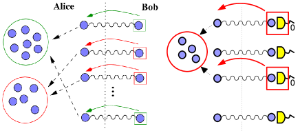
Figure 1: (Color online) Left: Alice separates her copies in two groups conditioned on an even (green) or odd (red) parity result obtained by Bob. Right: Alice selects copies corresponding to Bob’s no-photon results.

Alice’s even group can be described by the non-normalized density matrix $\rho_{1}^{e}=\mbox{Tr}_{2}\left\{P^{e}_{2}\rho_{12}P^{e}_{2}\right\}=\sum_{n=0}^{\infty}\,{}_{2}\langle 2n|\rho_{12}|2n\rangle_{2}$, where $P^{e}_{2}=\mathcal{I}_{1}\otimes\sum_{n=0}^{\infty}|2n\rangle_{2}\,{}_{2}\langle 2n|$, $\mathcal{I}_{1}$ the identity operator, and $|n\rangle_{2}$ the $n$-th Fock state for mode $2$. Using a similar notation, Alice’s odd group is given as $\rho_{1}^{o}=\mbox{Tr}_{2}\left\{P^{o}_{2}\rho_{12}P^{o}_{2}\right\}=\sum_{n=0}^{\infty}\,{}_{2}\langle 2n+1|\rho_{12}|2n+1\rangle_{2}$. But one can show that haruna2 $\sigma_{1}=2\sqrt{\mbox{det}(\mathbf{V}_{2})}(\rho_{1}^{e}\,-\,\rho_{1}^{o})=\int\mathrm{d}\mathbf{z_{1}}\mathrm{e}^{\mathbf{z_{1}^{\dagger}}\mathbf{Z}\mathbf{a}_{1}}\mathrm{e}^{-\frac{1}{2}\mathbf{z_{1}^{\dagger}}\mathbf{\Gamma_{1}}\mathbf{z_{1}}},$ where $\mathrm{d}\mathbf{z_{1}}=(1/\pi)\mathrm{d}\mbox{Re}(z_{1})\mathrm{d}\mbox{Im}(z_{1})$ and $\mathbf{\Gamma_{1}}$ is the Schur complement horn of $\mathbf{V_{2}}$:

$${\bf\Gamma}_{1}=\textbf{V}_{1}-\textbf{C}\textbf{V}_{2}^{-1}\textbf{C}^{\dagger}=\left(\begin{array}[]{cc}\eta_{1}&\mu_{1}\\ \mu_{1}^{*}&\eta_{1}\end{array}\right).$$ (2)

However, any one-mode Gaussian operator can be written as $\int\mathrm{d}\mathbf{z_{1}}\mathrm{e}^{\mathbf{z_{1}^{\dagger}}\mathbf{Z}\mathbf{a}_{1}}\mathrm{e}^{-\frac{1}{2}\mathbf{z_{1}^{\dagger}}\mathbf{\Gamma}_{1}\mathbf{z_{1}}}$, being $\mathbf{\Gamma}_{1}$ its covariance matrix englert . Therefore, $\sigma_{1}$ is a Gaussian operator whose covariance matrix elements are $\eta_{1}=2\sqrt{\mbox{det}(\mathbf{V}_{2})}(\langle a_{1}^{\dagger}a_{1}\rangle_{e}-\langle a_{1}^{\dagger}a_{1}\rangle_{o})$ and $\mu_{1}=2\sqrt{\mbox{det}(\mathbf{V}_{2})}(\langle a_{1}^{2}\rangle_{e}-\langle a_{1}^{2}\rangle_{o}),$ where $\langle\cdot\rangle_{e}=\mbox{Tr}(\cdot\rho_{1}^{e})$ and $\langle\cdot\rangle_{o}=\mbox{Tr}(\cdot\rho_{1}^{o})$. Summing up, $\mathbf{\Gamma}_{1}$ can be obtained with the knowledge of $\mbox{det}(\mathbf{V}_{2})$ and the second moments of $\rho_{1}^{e}$ and $\rho_{1}^{o}$, all of which determined via LOCC nonGaussian . Defining $\gamma=(n_{1}-\eta_{1})\left(n_{2}^{2}-|m_{2}|^{2}\right)$ and $\delta=(m_{1}-\mu_{1})\left(n_{2}^{2}-|m_{2}|^{2}\right)$, Eq. (2) gives two independent equations, which alone cannot give $m_{s}$ and $m_{c}$ unequivocally:

$$\gamma = n_{2}\left(|m_{c}|^{2}+|m_{s}|^{2}\right)-2\mbox{Re}(m_{2}m_{s}m_{c}^{*}),$$ (3)

$$\delta = 2n_{2}m_{s}m_{c}-m_{2}^{*}m_{c}^{2}-m_{2}m_{s}^{2}.$$ (4)

A unique solution though can be obtained if we consider an additional subensemble on which Bob performs another kind of projective measurement. The results of this measurement are communicated to Alice who build a local covariance matrix that is related to the original one through the Schur complement structure, similar to (2). In the present case we consider the simplest choice, i.e., Bob is able to perform a vacuum state projection on his copies: photon-number measurements with no outcome. For each measurement, Bob informs Alice to which copies a no-photon result ($\rho_{2}\rightarrow|0\rangle_{2}\,{}_{2}\langle 0|$) occurred. Alice, then, proceeds in a similar fashion as before but considering only the vacuum projected subensemble (right of Fig. 1), described by the density matrix $\rho_{1}^{vac}=\mbox{Tr}_{2}(|0\rangle_{2}\,{}_{2}\langle 0|\rho_{12})/\mbox{Tr}_{12}(|0\rangle_{2}\,{}_{2}\langle 0|\rho_{12})$. One can show that haruna2 $\rho_{1}^{vac}=\int\mathrm{d}\mathbf{z_{1}}\mathrm{e}^{\mathbf{z_{1}^{\dagger}}\mathbf{Z}\mathbf{a}_{1}}\mathrm{e}^{-\frac{1}{2}\mathbf{z_{1}^{\dagger}}\mathbf{\Pi_{1}}\mathbf{z_{1}}}$, where

$${\bf\Pi}_{1}=\textbf{V}_{1}-\textbf{C}\left(\textbf{V}_{2}+\frac{1}{2}\textbf{I}\right)^{-1}\textbf{C}^{\dagger}=\left(\begin{array}[]{cc}\xi_{1}&\nu_{1}\\ \nu_{1}^{*}&\xi_{1}\end{array}\right),$$ (5)

with I the identity matrix of dimension two. Here, $\xi_{1}=\langle a_{1}^{\dagger}a_{1}\rangle_{vac}$ and $\nu_{1}=\langle a_{1}^{2}\rangle_{vac}$, where $\langle\cdot\rangle_{vac}=\mbox{Tr}(\cdot\rho_{1}^{vac})$. Explicitly, Eq. (5) gives us two more equations,

$$\alpha = \left(n_{2}+\frac{1}{2}\right)\left(|m_{c}|^{2}+|m_{s}|^{2}\right)-2\mbox{Re}(m_{2}m_{s}m_{c}^{*}),$$ (6)

$$\beta = 2\left(n_{2}+\frac{1}{2}\right)m_{s}m_{c}-m_{2}^{*}m_{c}^{2}-m_{2}m_{s}^{2},$$ (7)

in which $\alpha=(n_{1}-\xi_{1})((n_{2}+1/2)^{2}-|m_{2}|^{2})$ and $\beta=(m_{1}-\nu_{1})((n_{2}+1/2)^{2}-|m_{2}|^{2})$. It is worth to stress that $\alpha$ and $\beta$, as well as $\gamma$ and $\delta$, are functions of parameters locally obtained by Alice and Bob. In order to solve Eqs. (3), (4), (6), and (7) for $m_{c}$ and $m_{s}$ we write $m_{j}=|m_{j}|e^{i\theta_{j}},$ where $j=1,2,c,s$ and $\theta_{j}$ is real. In this notation, our task is to determine $\theta_{c}$, $\theta_{s}$, $|m_{c}|$, and $|m_{s}|$ with the aid of $\mathbf{\Gamma_{1}}$ and $\mathbf{\Pi_{1}}$, obtained by Alice via LOCC. The other quantities, $n_{1}$, $n_{2}$, $|m_{1}|$, $|m_{2}|$, $\theta_{1}$, and $\theta_{2}$ are easily obtained via local HM of modes $1$ and $2$.

(i) Determination of $\theta_{c}$ and $\theta_{s}$. Subtracting Eq. (4) from (7) we have $\beta-\delta=m_{s}m_{c},$ which gives

$$|m_{s}m_{c}| = |\beta-\delta|,$$ (8)

$$\theta_{s}+\theta_{c} = Arg(\beta-\delta),$$ (9)

where $Arg(z)$ is the phase of the complex number $z$. By the same token, subtracting Eq. (3) from (6) we have

$$|m_{c}|^{2}+|m_{s}|^{2}=2(\alpha-\gamma).$$ (10)

Inserting Eqs. (8) and (10) into (6) we get, $\alpha=(2n_{2}+1)(\alpha-\gamma)-2|m_{2}(\beta-\delta)|\cos(\theta_{2}+\theta_{s}-\theta_{c}).$ We could have used Eq. (3) as well. Solving, then, for $\theta_{s}-\theta_{c}$ we obtain,

$$\theta_{s}-\theta_{c}=\cos^{\!-1}\!\left[(\alpha n_{2}-\gamma(n_{2}+1/2))/|m_{2}(\beta-\delta)|\right]-\theta_{2}.$$ (11)

Eqs. (9) and (11) can be easily solved to give $\theta_{c}$ and $\theta_{s}$, the phases of $m_{c}$ and $m_{s}$. It is worth mentioning that Eq. (11) is only valid when $|(\beta-\delta)m_{2}|\neq 0$. Later we show how to overcome this limitation.

(ii) Determination of $|m_{c}|$ and $|m_{s}|$. From Eq. (10) we note that if we had $|m_{c}|^{2}-|m_{s}|^{2}$ the problem would be solved. Manipulating the real and imaginary parts of Eq. (7) we get

$$|m_{c}|^{2}-|m_{s}|^{2}=|\beta|\sin(\theta_{\beta}-\theta_{c}-\theta_{s})/[|m_{2}|\sin(\theta_{2}-\theta_{c}+\theta_{s})].$$ (12)

Here $\theta_{\beta}$ is the phase of $\beta$. Eqs. (10) and (12) can be directly solved to give $|m_{c}|$ and $|m_{s}|$, the moduli of $m_{c}$ and $m_{s}$. Eq. (12) is only valid for $|m_{2}\sin(\theta_{2}-\theta_{c}+\theta_{s})|\neq 0$. Thus, all the covariance matrix elements can be locally reconstructed with a set of appropriate measurements and classical communication, establishing the following important connection to Gaussian QST: Global QST is completely equivalent to local covariance matrix HM, local parity and vacuum state projections, and classical communication. This is our central result and in the rest of this Letter we show how the necessary conditions $|(\beta-\delta)m_{2}|\neq 0$ and $|m_{2}\sin(\theta_{2}-\theta_{c}+\theta_{s})|\neq 0$ can always be obtained by the addition of local squeezing localSqueezing .

(iii) Overcoming $|(\beta-\delta)m_{2}|=0$ or $|m_{2}\sin(\theta_{2}-\theta_{c}+\theta_{s})|=0$. To properly solve these problems we must know which quantity is zero. The simplest check is implemented when Bob reconstructs $\mathbf{V_{2}}$, which allows him to know if $m_{2}=0$. Alice and Bob can also discover if $m_{c}=m_{s}=0$ (implying $\beta-\delta=m_{s}m_{c}=0$) by testing if $\mathbf{V_{1}}=\mathbf{\Gamma_{1}}=\mathbf{\Pi_{1}}$, since the absence of correlation ($\mathbf{C}=0$) between the modes cannot change what the parties measure locally (See Eqs. (2) and (5)). Also, if $\mathbf{V_{1}}\neq\mathbf{\Gamma_{1}}$ or $\mathbf{V_{1}}\neq\mathbf{\Pi_{1}}$ Alice and Bob are sure that $\mathbf{C}\neq 0$ and the first non-trivial check sets in. They must discover if either $m_{c}=0$ and $m_{s}\neq 0$, or $m_{c}\neq 0$ and $m_{s}=0$, or both $m_{c}\neq 0$ and $m_{c}\neq 0$. If either $m_{c}$ or $m_{s}$ is zero it is obvious that $|I_{3}|=|\mbox{det}(\mathbf{C})|=||m_{s}|^{2}-|m_{c}|^{2}|=|m_{s}|^{2}+|m_{c}|^{2}.$ But one can show haruna that $|I_{3}|=\sqrt{\mbox{det}(\mathbf{V}_{2})\mbox{det}(\mathbf{V}_{1}-\mathbf{\Gamma}_{1})}$ and using Eq. (10) we see that if $|I_{3}|=2(\alpha-\gamma)$ we know for sure that either $m_{s}$ or $m_{c}$ is zero. If we do not have an equality $m_{c}\neq 0$ and $m_{s}\neq 0$. For our purposes, as we explain below, we do not need to know which quantity, $m_{c}$ or $m_{s}$, is zero footnoteEnt . Finally, to discover if $\sin(\theta_{2}-\theta_{c}+\theta_{s})=0$ we use Eq. (11) and the phase of $m_{2}$. Of course, Eq. (11) is only valid if $|m_{2}(\beta-\delta)|\neq 0$. Therefore, if $|m_{2}(\beta-\delta)|=0$ we first need to solve this problem in order to test if $\sin(\theta_{2}-\theta_{c}+\theta_{s})=0$. Since now we know which parameter is zero we are ready to show how Alice and Bob can overcome this situation allowing them to use Eqs. (9) to (12) to obtain $\mathbf{C}$. See Tab. 1 for an overview of the strategies to solve these problems.

Table 1: Overview of the general strategies. Here $j=2,s,c$.

	$m_{j}=0$	$\sin(\theta_{2}-\theta_{c}+\theta_{s})=0$
local squeezing	yes	yes
local quadrature rotation	no	yes

If $m_{2}=0$ the most general solution footnoteM2 is achieved implementing a local symplectic transformation (local quadrature squeezing and rotation) on mode $2$ Sim94 , $\mathbf{S}=\mbox{diag}(\mathbf{I}_{1},\mathbf{S_{2}})$, where $\mathbf{I}_{1}$ is a $2\times 2$ identity matrix acting on system 1 and $\mathbf{S}_{2}$ is given as

$$\mathbf{S}_{2}=\left(\begin{array}[]{cc}e^{-is_{2}}\cosh r_{2}&\sinh r_{2}\\ \sinh r_{2}&e^{is_{2}}\cosh r_{2}\end{array}\right),$$ (13)

being $s_{2}$ and $r_{2}$ real parameters. The new correlation matrix $\tilde{\mathbf{V}}$ is connected to $\mathbf{V}$ by $\tilde{\mathbf{V}}=\mathbf{S}\mathbf{V}\mathbf{S^{\dagger}}$ Sim94 , or equivalently for $j=1,2$,$\mathbf{\tilde{V}}\!_{j}=\mathbf{S}_{j}\mathbf{V}\!_{j}\,\mathbf{S^{\dagger}}\!_{j},\mathbf{\tilde{C}}=\mathbf{S}_{1}\mathbf{C}\mathbf{S^{\dagger}}\!_{2}.$ Applying $\mathbf{S}$ to (1), the off-diagonal term of $\tilde{V}_{2}$ is $\tilde{m}_{2}=\mathrm{e}^{-2is_{2}}m_{2}\cosh^{2}r_{2}+m_{2}^{*}\sinh^{2}r_{2}+\mathrm{e}^{-is_{2}}n_{2}\sinh(2r_{2}).$ Setting $s_{2}=0$ and using that $m_{2}=0$ we have

$$\tilde{m}_{2}=n_{2}\sinh(2r_{2}),$$ (14)

i.e., a new covariance matrix with $\tilde{m}_{2}\neq 0$. After this operation we can proceed with the original protocol to reconstruct $\mathbf{\tilde{V}}$, which can be transformed back to give $\mathbf{V}=\mathbf{S}^{-1}\mathbf{\tilde{V}}\mathbf{S^{\dagger}}^{-1}$, with $\mathbf{S}^{-1}=\mbox{diag}\left(\mathbf{I}_{1},\mathbf{S}_{2}^{-1}\right)$ and

$$\mathbf{S}_{2}^{-1}=\left(\begin{array}[]{cc}e^{is_{2}}\cosh r_{2}&-\sinh r_{2}\\ -\sinh r_{2}&e^{-is_{2}}\cosh r_{2}\end{array}\right).$$ (15)

If either $m_{s}=0$ or $m_{c}=0$, or equivalently $\beta-\delta=0$, we can obtain a new matrix $\tilde{\mathbf{C}}=\mathbf{S}_{1}\mathbf{C}\mathbf{S^{\dagger}}\!_{2}$ where both parameters are not zero via a local squeezing operation alone. This leads to

$$\tilde{m}_{s} = e^{is_{2}}m_{s}\cosh r_{2}+m_{c}\sinh r_{2},$$ (16)

$$\tilde{m}_{c} = e^{-is_{2}}m_{c}\cosh r_{2}+m_{s}\sinh r_{2}.$$ (17)

Setting $s_{2}=0$ in Eqs. (16) and (17) we see that $\tilde{m}_{s}$ and $\tilde{m}_{c}$ are combinations of $m_{s}$ and $m_{c}$. Therefore, if $m_{s}=0$ or $m_{c}=0$ the new coefficients are necessary different from zero whenever we apply a local squeezing operation on mode $2$. As anticipated, we do not need to know which quantity was originally zero. As before, after this local transformation we proceed with the original protocol obtaining $\mathbf{\tilde{V}}$ and then $\mathbf{V}$. It is worth noting that when the two situations occur simultaneously, i.e. $m_{2}=0$ and $m_{s}=0$ or $m_{c}=0$, the same local squeezing operation solves at once both problems, as can be seen in Eqs. (14), (16), and (17).

Lastly, after being sure that $|m_{2}m_{c}m_{s}|\neq 0$ we can proceed to test if $\sin(\theta_{2}-\theta_{c}+\theta_{s})=0$ using Eq. (11) and the phase of $m_{2}$, all quantities locally determined. In case of a positive result, there exist three possible solutions. The first one is valid when $m_{2}\neq m_{1}$ and is achieved reversing the roles of Alice and Bob in the protocol, as discussed above. The remaining two possibilities, and more general, is to locally and unitary transform mode $1$ or mode $2$ before we implement the protocol, in the same fashion as before. Therefore, we need to show that there exists at least one local unitary operation acting on mode $1$ or mode $2$ that eliminates such a problem.

Let us begin with mode $2$. Applying the symplectic local transformation $\mathbf{S_{2}}$ we get, after assuming that $\sin(\theta_{2}-\theta_{c}+\theta_{s})=0$,

$$\tan(\tilde{\theta}_{2}+\tilde{\theta}_{s}-\tilde{\theta}_{c})=2\mathcal{A}_{\pm}\sin(\theta_{2}-s_{2})\sinh(2r_{2})/\mathcal{B}_{\pm},$$ (18)

$$\mathcal{A}_{\pm} = |m_{2}|(|m_{c}|^{2}+|m_{s}|^{2})\mp 2n_{2}|m_{c}m_{s}|,$$ (19)

$$\mathcal{B}_{\pm} = \pm 3|m_{2}m_{c}m_{s}|-n_{2}(|m_{c}|^{2}+|m_{s}|^{2})$$ (20)

$$+(\pm|m_{2}m_{c}m_{s}|+n_{2}(|m_{c}|^{2}+|m_{s}|^{2}))\cosh(4r_{2})$$

$$\pm 2|m_{2}m_{c}m_{s}|\cos(2\theta_{2}-2s_{2})\sinh^{2}(2r_{2})$$

$$+\mathcal{A}_{\mp}\cos(\theta_{2}-s_{2})\sinh(4r_{2}).$$

Here $\mathcal{A}_{\pm}$ ($\mathcal{B}_{\pm}$) stand for the two possible values for the cosine, i.e., $\cos(\theta_{2}-\theta_{c}+\theta_{s})=\pm 1$, respectively. From Eqs. (18) and (19) we see that a local squeezing alone ($r_{2}\neq 0$ and $s_{2}=0$) on mode $2$ can make $\tan(\tilde{\theta}_{2}+\tilde{\theta}_{s}-\tilde{\theta}_{c})\neq 0$ if $m_{2}$ is not real ($\theta_{2}\neq 0$). However, whenever $m_{2}$ is real a rotation on the quadratures ($s_{2}\neq 0$) is mandatory. There is one last loophole to fix, namely, the rare instances in which $\mathcal{A}_{+}=0$ (note that $\mathcal{A}_{-}$ is always different from zero). This is fixed by allowing the other party, in this case Alice, to implement a local squeezing on mode $1$. As shown in Eqs. (16) and (17) this operation allows Alice to change at her will the phases of $m_{s}$ and $m_{c}$ without altering $\theta_{2}$, solving completely the last problem. By the way, this is the other possible solution for the $\sin(\theta_{2}-\theta_{c}+\theta_{s})=0$ case, i.e., a local squeezing directly on mode $1$.

In summary, we showed a strictly local protocol in which a two-mode Gaussian state is completely reconstructed without relying on simultaneous HM or non-local resources. Actually, the only resources needed for this protocol are the ability to perform single mode HM, local parity and vacuum projective measurements, and classical communication. We also showed the complete equivalence of this local protocol to QST for Gaussian states. This equivalence is important for quantum communication purposes since now we can achieve the same goals of QST without non-local resources and simultaneous HM. The set of local parity measurements required here, however, may restrict the implementation of the protocol, apart from instances where this measurement can be, in principle, performed gerry . Finally, this new protocol raises several interesting problems yet to be solved. Firstly, it is unknown if a similar local protocol can be devised for more than two modes and, secondly, if there exist other optimal sets of measurements, than parity and vacuum projections, allowing the complete state reconstruction of a two-mode (or many-mode) Gaussian (or non-Gaussian) state in a simpler local way.

References

• (1) S. L. Braunstein and P. van Loock, Rev. Mod. Phys. 77, 513 (2005).
• (2) K. Vogel and H. Risken, Phys. Rev. A 40, 2847 (1989).
• (3) D. T. Smithey et al., Phys Rev. Lett. 70, 1244 (1993).
• (4) M. Paris and J. Řeháček (Eds.), Quantum State Estimation, Lect. Notes Phys. 649 (Springer, Berlin Heidelberg, 2004).
• (5) M. Vasilyev et al., Phys. Rev. Lett. 84, 2354 (2000).
• (6) S. A. Babichev, J. Appel, and A. I. Lvovsky, Phys. Rev. Lett. 92, 193601 (2004).
• (7) W. P. Bowen et al., Phys. Rev. A 69, 012304 (2004).
• (8) E. L. Bolda, S. M. Tan, and D. F. Walls, Phys. Rev. Lett. 79, 4719 (1997); R. Walser, ibid. 79, 4724 (1997); M. G. Raymer and A. C. Funk, Phys. Rev. A 61, 015801 (1999); G. M. D’Ariano, M. F. Sacchi, and P. Kumar, Phys. Rev. A 61, 013806 (1999); D’Auria et al., J. Opt. B: Quant. Semiclass. Opt. 7, S750 (2005); J. Laurat et al., J. Opt. B: Quantum Semiclass. Opt. 7, s577 (2005).
• (9) V. D’Auria et. al., Phys. Rev. Lett. 102, 020502 (2009).
• (10) B. G. Englert and K. Wódkiewicz, Int. J. Quant. Inf. 1, 153 (2003).
• (11) G. Adesso and F. Illuminati, J. Phys. A: Math. Theor. 40, 7821 (2007); G. Adesso, arXiv:quant-ph/0702069v1.
• (12) This can be achieved through a local displacement operation without changing the states’ entanglement content.
• (13) L. F. Haruna, M. C. de Oliveira, and G. Rigolin, Phys. Rev. Lett. 98, 150501 (2007); L. F. Haruna, M. C. de Oliveira, and G. Rigolin, ibid. 99, 059902 (2007).
• (14) L.F. Haruna and M.C. de Oliveira, J. Phys. A: Math. Theor. 40, 14195 (2007).
• (15) R. A. Horn and C. R. Johnson, Matrix Analysis (Cambridge University Press, Cambridge, 1987).
• (16) We do not need to manipulate these non-Gaussian states; we just measure their covariance matrices.
• (17) For the non-trivial implementation of a local squeezing operation see R. Filip, P. Marek, and U.L. Andersen, Phys. Rev. A 71, 042308 (2005); J.-i. Yoshikawa et al., Phys. Rev. A 76, 060301(R) (2007).
• (18) We can discover which parameter is zero if the state is entangled because in this case $I_{3}<0$ simon , implying that $m_{s}=0$ and $m_{c}\neq 0$. To test for entanglement we use the Simon separability test simon : we have entanglement if, and only if, $I_{1}I_{2}+(1/4-|I_{3}|)^{2}-I_{4}<(I_{1}+I_{2})/4,$ with $I_{j}=\mbox{det}(\mathbf{V}_{j})$, $j=1,2$, $I_{4}=I_{1}I_{2}+I_{3}^{2}-I_{V}$, $I_{V}=\mbox{det}(\mathbf{V})=\mbox{det}(\mathbf{V}_{2})\mbox{det}(\mathbf{\Gamma}_{1});$ $\mathbf{C}$ is also readily attained since $|m_{c}|^{2}=\alpha/(n_{2}+1/2)=\gamma/n_{2}$ and $\theta_{c}=(\theta_{\beta}+\theta_{2}-\pi)/2=(\theta_{\delta}+\theta_{2}-\pi)/2$, where $\theta_{\delta}$ is the phase of $\delta$.
• (19) There is another solution when $m_{2}=0$ and $m_{1}\neq 0$ (non-symmetric Gaussian states). Here the problem is solved by exchanging the roles of Alice and Bob in the previous protocol: $m_{2}\leftrightarrow m_{1}$ and $n_{2}\leftrightarrow n_{1}$ in all expressions.
• (20) R. Simon, N. Mukunda, and B. Dutta, Phys. Rev. A 49, 1567 (1994).
• (21) R. Simon, Phys. Rev. Lett 84, 2726 (2000).
• (22) S. Haroche, M. Brune, and J.M. Raimond, J. Mod. Opt. 54, 2101 (2007); C.C. Gerry, A. Benmoussa, and R.A. Campos, Phys. Rev. A 72, 053818 (2005).