Algorithm Selection as a Bandit Problem with Unbounded Losses

Abstract

Algorithm selection is typically based on models of algorithm performance, learned during a separate offline training sequence, which can be prohibitively expensive. In recent work, we adopted an online approach, in which a performance model is iteratively updated and used to guide selection on a sequence of problem instances. The resulting exploration-exploitation trade-off was represented as a bandit problem with expert advice, using an existing solver for this game, but this required the setting of an arbitrary bound on algorithm runtimes, thus invalidating the optimal regret of the solver. In this paper, we propose a simpler framework for representing algorithm selection as a bandit problem, with partial information, and an unknown bound on losses. We adapt an existing solver to this game, proving a bound on its expected regret, which holds also for the resulting algorithm selection technique. We present preliminary experiments with a set of SAT solvers on a mixed SAT-UNSAT benchmark.

1 Introduction

Decades of research in the fields of Machine Learning and Artificial Intelligence brought us a variety of alternative algorithms for solving many kinds of problems. Algorithms often display variability in performance quality, and computational cost, depending on the particular problem instance being solved: in other words, there is no single “best” algorithm. While a “trial and error” approach is still the most popular, attempts to automate algorithm selection are not new [33], and have grown to form a consistent and dynamic field of research in the area of Meta-Learning [37]. Many selection methods follow an offline learning scheme, in which the availability of a large training set of performance data for the different algorithms is assumed. This data is used to learn a model that maps (problem, algorithm) pairs to expected performance, or to some probability distribution on performance. The model is later used to select and run, for each new problem instance, only the algorithm that is expected to give the best results. While this approach might sound reasonable, it actually ignores the computational cost of the initial training phase: collecting a representative sample of performance data has to be done via solving a set of training problem instances, and each instance is solved repeatedly, at least once for each of the available algorithms, or more if the algorithms are randomized. Furthermore, these training instances are assumed to be representative of future ones, as the model is not updated after training.

In other words, there is an obvious trade-off between the exploration of algorithm performances on different problem instances, aimed at learning the model, and the exploitation of the best algorithm/problem combinations, based on the model’s predictions. This trade-off is typically ignored in offline algorithm selection, and the size of the training set is chosen heuristically. In our previous work [13, 14, 15], we have kept an online view of algorithm selection, in which the only input available to the meta-learner is a set of algorithms, of unknown performance, and a sequence of problem instances that have to be solved. Rather than artificially subdividing the problem set into a training and a test set, we iteratively update the model each time an instance is solved, and use it to guide algorithm selection on the next instance.

Bandit problems [3] offer a solid theoretical framework for dealing with the exploration-exploitation trade-off in an online setting. One important obstacle to the straightforward application of a bandit problem solver to algorithm selection is that most existing solvers assume a bound on losses to be available beforehand. In [16, 15] we dealt with this issue heuristically, fixing the bound in advance. In this paper, we introduce a modification of an existing bandit problem solver [7], which allows it to deal with an unknown bound on losses, while retaining a bound on the expected regret. This allows us to propose a simpler version of the algorithm selection framework GambleTA, originally introduced in [15]. The result is a parameterless online algorithm selection method, the first, to our knowledge, with a provable upper bound on regret.

The rest of the paper is organized as follows. Section 2 describes a tentative taxonomy of algorithm selection methods, along with a few examples from literature. Section 3 presents our framework for representing algorithm selection as a bandit problem, discussing the introduction of a higher level of selection among different algorithm selection techniques (time allocators). Section 4 introduces the modified bandit problem solver for unbounded loss games, along with its bound on regret. Section 5 describes experiments with SAT solvers. Section 6 concludes the paper.

2 Related work

In general terms, algorithm selection can be defined as the process of allocating computational resources to a set of alternative algorithms, in order to improve some measure of performance on a set of problem instances. Note that this definition includes parameter selection: the algorithm set can contain multiple copies of a same algorithm, differing in their parameter settings; or even identical randomized algorithms differing only in their random seeds. Algorithm selection techniques can be further described according to different orthogonal features:

Decision vs. optimisation problems. A first distinction needs to be made among decision problems, where a binary criterion for recognizing a solution is available; and optimisation problems, where different levels of solution quality can be attained, measured by an objective function [22]. Literature on algorithm selection is often focused on one of these two classes of problems. The selection is normally aimed at minimizing solution time for decision problems; and at maximizing performance quality, or improving some speed-quality trade-off, for optimisation problems.
Per set vs. per instance selection. The selection among different algorithms can be performed once for an entire set of problem instances (per set selection, following [24]); or repeated for each instance (per instance selection).
Static vs. dynamic selection. A further independent distinction [31] can be made among static algorithm selection, in which allocation of resources precedes algorithm execution; and dynamic, or reactive, algorithm selection, in which the allocation can be adapted during algorithm execution.
Oblivious vs. non-oblivious selection. In oblivious techniques, algorithm selection is performed from scratch for each problem instance; in non-oblivious techniques, there is some knowledge transfer across subsequent problem instances, usually in the form of a model of algorithm performance.
Off-line vs. online learning. Non-oblivious techniques can be further distinguished as offline or batch learning techniques, where a separate training phase is performed, after which the selection criteria are kept fixed; and online techniques, where the criteria can be updated every time an instance is solved.

A seminal paper in the field of algorithm selection is [33], in which offline, per instance selection is first proposed, for both decision and optimisation problems. More recently, similar concepts have been proposed, with different terminology (algorithm recommendation, ranking, model selection), in the Meta-Learning community [12, 37, 18]. Research in this field usually deals with optimisation problems, and is focused on maximizing solution quality, without taking into account the computational aspect. Work on Empirical Hardness Models [27, 30] is instead applied to decision problems, and focuses on obtaining accurate models of runtime performance, conditioned on numerous features of the problem instances, as well as on parameters of the solvers [24]. The models are used to perform algorithm selection on a per instance basis, and are learned offline: online selection is advocated in [24]. Literature on algorithm portfolios [23, 19, 32] is usually focused on choice criteria for building the set of candidate solvers, such that their areas of good performance do not overlap, and optimal static allocation of computational resources among elements of the portfolio.

A number of interesting dynamic exceptions to the static selection paradigm have been proposed recently. In [25], algorithm performance modeling is based on the behavior of the candidate algorithms during a predefined amount of time, called the observational horizon, and dynamic context-sensitive restart policies for SAT solvers are presented. In both cases, the model is learned offline. In a Reinforcement Learning [36] setting, algorithm selection can be formulated as a Markov Decision Process: in [26], the algorithm set includes sequences of recursive algorithms, formed dynamically at run-time solving a sequential decision problem, and a variation of Q-learning is used to find a dynamic algorithm selection policy; the resulting technique is per instance, dynamic and online. In [31], a set of deterministic algorithms is considered, and, under some limitations, static and dynamic schedules are obtained, based on dynamic programming. In both cases, the method presented is per set, offline.

An approach based on runtime distributions can be found in [10, 11], for parallel independent processes and shared resources respectively. The runtime distributions are assumed to be known, and the expected value of a cost function, accounting for both wall-clock time and resources usage, is minimized. A dynamic schedule is evaluated offline, using a branch-and-bound algorithm to find the optimal one in a tree of possible schedules. Examples of allocation to two processes are presented with artificially generated runtimes, and a real Latin square solver. Unfortunately, the computational complexity of the tree search grows exponentially in the number of processes.

“Low-knowledge” oblivious approaches can be found in [4, 5], in which various simple indicators of current solution improvement are used for algorithm selection, in order to achieve the best solution quality within a given time contract. In [5], the selection process is dynamic: machine time shares are based on a recency-weighted average of performance improvements. We adopted a similar approach in [13], where we considered algorithms with a scalar state, that had to reach a target value. The time to solution was estimated based on a shifting-window linear extrapolation of the learning curves.

For optimisation problems, if selection is only aimed at maximizing solution quality, the same problem instance can be solved multiple times, keeping only the best solution. In this case, algorithm selection can be represented as a Max $K$-armed bandit problem, a variant of the game in which the reward attributed to each arm is the maximum payoff on a set of rounds. Solvers for this game are used in [9, 35] to implement oblivious per instance selection from a set of multi-start optimisation techniques: each problem is treated independently, and multiple runs of the available solvers are allocated, to maximize performance quality. Further references can be found in [15].

3 Algorithm selection as a bandit problem

In its most basic form [34], the multi-armed bandit problem is faced by a gambler, playing a sequence of trials against an $N$-armed slot machine. At each trial, the gambler chooses one of the available arms, whose losses are randomly generated from different stationary distributions. The gambler incurs in the corresponding loss, and, in the full information game, she can observe the losses that would have been paid pulling any of the other arms. A more optimistic formulation can be made in terms of positive rewards. The aim of the game is to minimize the regret, defined as the difference between the cumulative loss of the gambler, and the one of the best arm. A bandit problem solver (BPS) can be described as a mapping from the history of the observed losses $l_{j}$ for each arm $j$, to a probability distribution $\mathbf{p}=(p_{1},...,p_{N})$, from which the choice for the successive trial will be picked.

More recently, the original restricting assumptions have been progressively relaxed, allowing for non-stationary loss distributions, partial information (only the loss for the pulled arm is observed), and adversarial bandits that can set their losses in order to deceive the player. In [2, 3], a reward game is considered, and no statistical assumptions are made about the process generating the rewards, which are allowed to be an arbitrary function of the entire history of the game (non-oblivious adversarial setting). Based on these pessimistic hypotheses, the authors describe probabilistic gambling strategies for the full and the partial information games.

Let us now see how to represent algorithm selection for decision problems as a bandit problem, with the aim of minimizing solution time. Consider a sequence $\mathcal{B}=\{b_{1},\ldots,b_{M}\}$ of $M$ instances of a decision problem, for which we want to minimize solution time, and a set of $K$ algorithms $\mathcal{A}=\{a_{1},\ldots,a_{K}\}$, such that each $b_{m}$ can be solved by each $a_{k}$. It is straightforward to describe static algorithm selection in a multi-armed bandit setting, where “pick arm $k$” means “run algorithm $a_{k}$ on next problem instance”. Runtimes $t_{k}$ can be viewed as losses, generated by a rather complex mechanism, i.e., the algorithms $a_{k}$ themselves, running on the current problem. The information is partial, as the runtime for other algorithms is not available, unless we decide to solve the same problem instance again. In a worst case scenario one can receive a ”deceptive” problem sequence, starting with problem instances on which the performance of the algorithms is misleading, so this bandit problem should be considered adversarial. As BPS  typically minimize the regret with respect to a single arm, this approach would allow to implement per set selection, of the overall best algorithm. An example can be found in [16], where we presented an online method for learning a per set estimate of an optimal restart strategy.

Unfortunately, per set selection is only profitable if one of the algorithms dominates the others on all problem instances. This is usually not the case: it is often observed in practice that different algorithms perform better on different problem instances. In this situation, a per instance selection scheme, which can take a different decision for each problem instance, can have a great advantage.

One possible way of exploiting the nice theoretical properties of a BPS  in the context of algorithm selection, while allowing for the improvement in performance of per instance selection, is to use the BPS  at an upper level, to select among alternative algorithm selection techniques. Consider again the algorithm selection problem represented by $\mathcal{B}$ and $\mathcal{A}$. Introduce a set of $N$ time allocators ($\mbox{TA}_{j}$) [13, 15]. Each $\mbox{TA}_{j}$ can be an arbitrary function, mapping the current history of collected performance data for each $a_{k}$, to a share $\mathbf{s}^{(j)}\in[0,1]^{K}$, with $\sum_{k=1}^{K}s_{k}=1$. A TA is used to solve a given problem instance executing all algorithms in $\mathcal{A}$ in parallel, on a single machine, whose computational resources are allocated to each $a_{k}$ proportionally to the corresponding $s_{k}$, such that for any portion of time spent $t$, $s_{k}t$ is used by $a_{k}$, as in a static algorithm portfolio [23]. The runtime before a solution is found is then $\min_{k}\{t_{k}/s_{k}\}$, $t_{k}$ being the runtime of algorithm $a_{k}$.

A trivial example of a TA is the uniform time allocator, assigning a constant $\mathbf{s}=(1/K,...,1/K)$. Single algorithm selection can be represented in this framework by setting a single $s_{k}$ to $1$. Dynamic allocators will produce a time-varying share $\mathbf{s}(t)$. In previous work, we presented examples of heuristic oblivious [13] and non-oblivious [14] allocators; more sound TAs are proposed in [15], based on non-parametric models of the runtime distribution of the algorithms, which are used to minimize the expected value of solution time, or a quantile of this quantity, or to maximize solution probability within a give time contract.

At this higher level, one can use a BPS to select among different time allocators, $\mbox{TA}_{j},\mbox{TA}_{2}\ldots$, working on a same algorithm set $\mathcal{A}$. In this case, “pick arm $j$” means “use time allocator $\mbox{TA}_{j}$ on $\mathcal{A}$ to solve next problem instance”. In the long term, the BPS  would allow to select, on a per set basis, the $\mbox{TA}_{j}$ that is best at allocating time to algorithms in $\mathcal{A}$ on a per instance basis. The resulting “Gambling” Time Allocator (GambleTA) is described in Alg. 1.

Algorithm 1 GambleTA$(\mathcal{A},\mathcal{T},BPS)$ Gambling Time Allocator.

  Algorithm set $\mathcal{A}$ with $K$ algorithms;

  A set $\mathcal{T}$ of $N$ time allocators $\mbox{TA}_{j}$;

  A bandit problem solver BPS 

  $M$ problem instances.

  

  initialize BPS$(N,M)$

  for each problem $b_{i},i=1,\ldots,M$ do

     pick time allocator $I(i)=j$ with probability $p_{j}(i)$ from BPS.

     solve problem $b_{i}$ using $\mbox{TA}_{I}$ on $\mathcal{A}$

     incur loss $l_{I(i)}=\min_{k}\{t_{k}(i)/s_{k}^{(I)}(i)\}$

     update BPS 

  end for

If BPS  allows for non-stationary arms, it can also deal with time allocators that are learning to allocate time. This is actually the original motivation for adopting this two-level selection scheme, as it allows to combine in a principled way the exploration of algorithm behavior, which can be represented by the uniform time allocator, and the exploitation of this information by a model-based allocator, whose model is being learned online, based on results on the sequence of problems met so far. If more time allocators are available, they can be made to compete, using the BPS  to explore their performances. Another interesting feature of this selection scheme is that the initial requirement that each algorithm should be capable of solving each problem can be relaxed, requiring instead that at least one of the $a_{k}$ can solve a given $b_{m}$, and that each $\mbox{TA}_{j}$ can solve each $b_{m}$: this can be ensured in practice by imposing a $s_{k}>0$ for all $a_{k}$. This allows to use interesting combinations of complete and incomplete solvers in $\mathcal{A}$ (see Sect. 5). Note that any bound on the regret of the BPS will determine a bound on the regret of GambleTA with respect to the best time allocator. Nothing can be said about the performance w.r.t. the best algorithm. In a worst-case setting, if none of the time allocator is effective, a bound can still be obtained by including the uniform share in the set of TAs. In practice, though, per-instance selection can be much more efficient than uniform allocation, and the literature is full of examples of time allocators which eventually converge to a good performance.

The original version of GambleTA  (GambleTA4 in the following) [15] was based on a more complex alternative, inspired by the bandit problem with expert advice, as described in [2, 3]. In that setting, two games are going on in parallel: at a lower level, a partial information game is played, based on the probability distribution obtained mixing the advice of different experts, represented as probability distributions on the $K$ arms. The experts can be arbitrary functions of the history of observed rewards, and give a different advice for each trial. At a higher level, a full information game is played, with the $N$ experts playing the roles of the different arms. The probability distribution $\mathbf{p}$ at this level is not used to pick a single expert, but to mix their advices, in order to generate the distribution for the lower level arms. In GambleTA4, the time allocators play the role of the experts, each suggesting a different $\mathbf{s}$, on a per instance basis; and the arms of the lower level game are the $K$ algorithms, to be run in parallel with the mixture share. Exp4  [2, 3] is used as the BPS. Unfortunately, the bounds for Exp4  cannot be extended to GambleTA4  in a straightforward manner, as the loss function itself is not convex; moreover, Exp4  cannot deal with unbounded losses, so we had to adopt an heuristic reward attribution instead of using the plain runtimes.

A common issue of the above approaches is the difficulty of setting reasonable upper bounds on the time required by the algorithms. This renders a straightforward application of most BPS  problematic, as a known bound on losses is usually assumed, and used to tune parameters of the solver. Underestimating this bound can invalidate the bounds on regret, while overestimating it can produce an excessively ”cautious” algorithm, with a poor performance. Setting in advance a good bound is particularly difficult when dealing with algorithm runtimes, which can easily exhibit variations of several order of magnitudes among different problem instances, or even among different runs on a same instance [20].

Some interesting results regarding games with unbounded losses have recently been obtained. In [7, 8], the authors consider a full information game, and provide two algorithms which can adapt to unknown bounds on signed rewards. Based on this work, [1] provide a Hannan consistent algorithm for losses whose bound grows in the number of trials $i$ with a known rate $i^{\nu}$, $\nu<1/2$. This latter hypothesis does not fit well our situation, as we would like to avoid any restriction on the sequence of problems: a very hard instance can be met first, followed by an easy one. In this sense, the hypothesis of a constant, but unknown, bound is more suited. In [7], Cesa-Bianchi et al. also introduce an algorithm for loss games with partial information (Exp3Light), which requires losses to be bound, and is particularly effective when the cumulative loss of the best arm is small. In the next section we introduce a variation of this algorithm that allows it to deal with an unknown bound on losses.

4 An algorithm for games with an unknown bound on losses

Here and in the following, we consider a partial information game with $N$ arms, and $M$ trials; an index $(i)$ indicates the value of a quantity used or observed at trial $i\in\{1,\ldots,M\}$; $j$ indicate quantities related to the $j$-th arm, $j\in\{1,\ldots,N\}$; index $E$ refers to the loss incurred by the bandit problem solver, and $I(i)$ indicates the arm chosen at trial $(i)$, so it is a discrete random variable with value in $\{1,\ldots,N\}$; $r$, $u$ will represent quantities related to an epoch of the game, which consists of a sequence of $0$ or more consecutive trials; $\log$ with no index is the natural logarithm.

Exp3Light  [7, Sec. 4] is a solver for the bandit loss game with partial information. It is a modified version of the weighted majority algorithm [29], in which the cumulative losses for each arm are obtained through an unbiased estimate. The game consists of a sequence of epochs $r=0,1,\ldots$: in each epoch, the probability distribution over the arms is updated, proportional to $\exp{(-\eta_{r}\tilde{L}_{j})}$, $\tilde{L}_{j}$ being the current unbiased estimate of the cumulative loss. Assuming an upper bound $4^{r}$ on the smallest loss estimate, $\eta_{r}$ is set as:

$$\eta_{r}=\sqrt{\frac{2(\log N+N\log M)}{(N4^{r})}}$$ (1)

When this bound is first trespassed, a new epoch starts and $r$ and $\eta_{r}$ are updated accordingly.

Algorithm 2 Exp3Light$(N,M,\mathcal{L})$ A solver for bandit problems with partial information and a known bound $\mathcal{L}$ on losses.

  $N$ arms, $M$ trials

  losses $l_{j}(i)\in[0,\mathcal{L}]$ $\forall$ $i=1,...,M$, $j=1,\ldots,N$

  initialize epoch $r=0$, $L_{E}=0$, $\tilde{L}_{j}(0)=0$.

  initialize $\eta_{r}$ according to (1)

  for each trial $i=1,...,M$ do

     set $p_{j}(i)\propto\exp(-\eta_{r}\tilde{L}_{j}(i-1)/\mathcal{L})$, $\sum_{j=1}^{N}p_{j}(i)=1$.

     pick arm $I(i)=j$ with probability $p_{j}(i)$.

     incur loss $l_{E}(i)=l_{I(i)}(i)$.

     evaluate unbiased loss estimates:

     $\tilde{l}_{I(i)}(i)=l_{I(i)}(i)/p_{I(i)}(i)$, $\tilde{l}_{j}=0$ for $j\neq I(i)$

     update cumulative losses:

     $L_{E}(i)=L_{E}(i-1)+l_{E}(i)$,

     $\tilde{L}_{j}(i)=\tilde{L}_{j}(i-1)+\tilde{l}_{j}(i)$, for $j=1,\ldots,N$

     $\tilde{L}^{*}(i)=min_{j}\tilde{L}_{j}(i)$.

     if $(\tilde{L}^{*}(i)/\mathcal{L})>4^{r}$ then

        start next epoch $r=\lceil\log_{4}(\tilde{L}^{*}(i)/\mathcal{L})\rceil$

        update $\eta_{r}$ according to (1)

     end if

  end for

The original algorithm assumes losses in $[0,1]$. We first consider a game with a known finite bound $\mathcal{L}$ on losses, and introduce a slightly modified version of Exp3Light  (Algorithm 2), obtained simply dividing all losses by $\mathcal{L}$. Based on Theorem 5 from [7], it is easy to prove the following

Theorem 1.

If $L^{*}(M)$ is the loss of the best arm after $M$ trials, and $L_{E}(M)=\sum_{i=1}^{M}l_{I(i)}(i)$ is the loss of Exp3Light$(N,M,\mathcal{L})$, the expected value of its regret is bounded as:

$$E\{L_{E}(M)\}-L^{*}(M)$$

$$\leq 2\sqrt{6\mathcal{L}(\log N+N\log M)NL^{*}(M)}$$

$$+ \mathcal{L}[2\sqrt{2\mathcal{L}(\log N+N\log M)N}$$

$$+ (2N+1)(1+\log_{4}(3M+1))]$$

The proof is trivial, and is given in the appendix.

We now introduce a simple variation of Algorithm 2 which does not require the knowledge of the bound $\mathcal{L}$ on losses, and uses Algorithm 2 as a subroutine. Exp3Light-A  (Algorithm 3) is inspired by the doubling trick used in [7] for a full information game with unknown bound on losses. The game is again organized in a sequence of epochs $u=0,1,\ldots$: in each epoch, Algorithm 2 is restarted using a bound $\mathcal{L}_{u}=2^{u}$; a new epoch is started with the appropriate $u$ whenever a loss larger than the current $\mathcal{L}_{u}$ is observed.

Algorithm 3 Exp3Light-A$(N,M)$ A solver for bandit problems with partial information and an unknown (but finite) bound on losses.

  $N$ arms, $M$ trials,

  losses $l_{j}(i)\in[0,\mathcal{L}]$ $\forall$ $i=1,...,M$,$j=1,\ldots,N$

  unknown $\mathcal{L}<\infty$

  initialize epoch $u=0$, Exp3Light$(N,M,2^{u})$

  for each trial $i=1,...,M$ do

     pick arm $I(i)=j$ with probability $p_{j}(i)$ from Exp3Light.

     incur loss $l_{E}(i)=l_{I(i)}(i)$.

     if $l_{I(i)}(i)>2^{u}$ then

        start next epoch $u=\lceil\log_{2}l_{I(i)}(i)\rceil$

        restart Exp3Light$(N,M-i,2^{u})$

     end if

  end for

Theorem 2.

If $L^{*}(M)$ is the loss of the best arm after $M$ trials, and $\mathcal{L}<\infty$ is the unknown bound on losses, the expected value of the regret of Exp3Light-A$(N,M)$ is bounded as:

$$E\{L_{E}(M)\}-L^{*}(M)\leq$$

$$4\sqrt{3\lceil\log_{2}\mathcal{L}\rceil\mathcal{L}(\log N+N\log M)NL^{*}(M)}$$

$$+ 2\lceil\log_{2}\mathcal{L}\rceil\mathcal{L}[\sqrt{4\mathcal{L}(\log N+N\log M)N}$$

$$+ (2N+1)(1+\log_{4}(3M+1))+2]$$

The proof is given in the appendix. The regret obtained by Exp3Light-A  is $O(\sqrt{\mathcal{L}N\log ML^{*}(M)})$, which can be useful in a situation in which $\mathcal{L}$ is high but $L^{*}$ is relatively small, as we expect in our time allocation setting if the algorithms exhibit huge variations in runtime, but at least one of the TAs eventually converges to a good performance. We can then use Exp3Light-A  as a BPS  for selecting among different time allocators in GambleTA  (Algorithm 1).

5 Experiments

The set of time allocator used in the following experiments is the same as in [15], and includes the uniform allocator, along with nine other dynamic allocators, optimizing different quantiles of runtime, based on a nonparametric model of the runtime distribution that is updated after each problem is solved. We first briefly describe these time allocators, inviting the reader to refer to [15] for further details and a deeper discussion. A separate model $F_{k}(t|\mathbf{x})$, conditioned on features $\mathbf{x}$ of the problem instance, is used for each algorithm $a_{k}$. Based on these models, the runtime distribution for the whole algorithm portfolio $\mathcal{A}$ can be evaluated for an arbitrary share $\mathbf{s}\in[0,1]^{K}$, with $\sum_{k=1}^{K}s_{k}=1$, as

$$F_{\mathcal{A},\mathbf{s}}(t)=1-\prod_{k=1}^{K}[1-F_{k}(s_{k}t)].$$ (4)

Eq. (4) can be used to evaluate a quantile $t_{\mathcal{A},\mathbf{s}}(\alpha)=F_{\mathcal{A},\mathbf{s}}^{-1}(\alpha)$ for a given solution probability $\alpha$. Fixing this value, time is allocated using the share that minimizes the quantile

$$\mathbf{s}=\arg\min_{\mathbf{s}}F_{\mathcal{A},\mathbf{s}}^{-1}(\alpha).$$ (5)

Compared to minimizing expected runtime, this time allocator has the advantage of being applicable even when the runtime distributions are improper, i. e. $F(\infty)<1$, as in the case of incomplete solvers. A dynamic version of this time allocator is obtained updating the share value periodically, conditioning each $F_{k}$ on the time spent so far by the corresponding $a_{k}$.

Rather than fixing an arbitrary $\alpha$, we used nine different instances of this time allocator, with $\alpha$ ranging from $0.1$ to $0.9$, in addition to the uniform allocator, and let the BPS  select the best one.

We present experiments for the algorithm selection scenario from [15], in which a local search and a complete SAT solver (respectively, G2-WSAT [28] and Satz-Rand [20]) are combined to solve a sequence of random satisfiable and unsatisfiable problems (benchmarks uf-*, uu-* from [21], $1899$ instances in total). As the clauses-to-variable ratio is fixed in this benchmark, only the number of variables, ranging from $20$ to $250$, was used as a problem feature $\mathbf{x}$. Local search algorithms are more efficient on satisfiable instances, but cannot prove unsatisfiability, so are doomed to run forever on unsatisfiable instances; while complete solvers are guaranteed to terminate their execution on all instances, as they can also prove unsatisfiability.

For the whole problem sequence, the overhead of GambleTA3  (Algorithm 1, using Exp3Light-A  as the BPS) over an ideal “oracle”, which can predict and run only the fastest algorithm, is $22\%$. GambleTA4 (from [15], based on Exp4) seems to profit from the mixing of time allocation shares, obtaining a better $14\%$. Satz-Rand alone can solve all the problems, but with an overhead of about $40\%$ w.r.t. the oracle, due to its poor performance on satisfiable instances. Fig. 1 plots the evolution of cumulative time, and cumulative overhead, along the problem sequence.

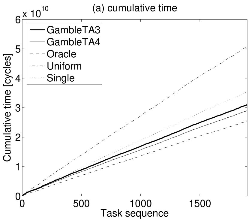
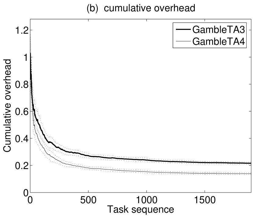
Figure 1: (a): Cumulative time spent by GambleTA3  and GambleTA4 [15] on the SAT-UNSAT problem set ($10^{9}\approx 1$ min.). Upper $95\%$ confidence bounds on $20$ runs, with random reordering of the problems. Oracle is the lower bound on performance. Uniform  is the ($0.5$,$0.5$) share. Satz-Rand is the per-set best algorithm. (b): The evolution of cumulative overhead, defined as $(\sum_{j}t_{G}(j)-\sum_{j}t_{O}(j))/\sum_{j}t_{O}(j)$, where $t_{G}$ is the performance of GambleTA  and $t_{O}$ is the performance of the oracle. Dotted lines represent $95\%$ confidence bounds.

6 Conclusions

We presented a bandit problem solver for loss games with partial information and an unknown bound on losses. The solver represents an ideal plug-in for our algorithm selection method GambleTA, avoiding the need to set any additional parameter. The choice of the algorithm set and time allocators to use is still left to the user. Any existing selection technique, including oblivious ones, can be included in the set of $N$ allocators, with an impact $O(\sqrt{N})$ on the regret: the overall performance of GambleTA  will converge to the one of the best time allocator. Preliminary experiments showed a degradation in performance compared to the heuristic version presented in [15], which requires to set in advance a maximum runtime, and cannot be provided of a bound on regret.

According to [6], a bound for the original Exp3Light  can be proved for an adaptive $\eta_{r}$ (1), in which the total number of trials $M$ is replaced by the current trial $i$. This should allow for a potentially more efficient variation of Exp3Light-A, in which Exp3Light  is not restarted at each epoch, and can retain the information on past losses.

One potential advantage of offline selection methods is that the initial training phase can be easily parallelized, distributing the workload on a cluster of machines. Ongoing research aims at extending GambleTA  to allocate multiple CPUs in parallel, in order to obtain a fully distributed algorithm selection framework [17].

Acknowledgments. We would like to thank Nicolò Cesa-Bianchi for contributing the proofs for Exp3Light and useful remarks on his work, and Faustino Gomez for his comments on a draft of this paper. This work was supported by the Hasler foundation with grant n. $2244$.

Appendix

A.1 Proof of Theorem 1

The proof is trivially based on the regret for the original Exp3Light, with $\mathcal{L}=1$, which according to [7, Theorem 5] (proof obtained from [6]) can be evaluated using the optimal values (1) for $\eta_{r}$ :

$$E\{L_{E}(M)\}-L^{*}(M)\leq$$

$$2\sqrt{2(\log N+N\log M)N(1+3L^{*}(M))}$$

$$+ (2N+1)(1+\log_{4}(3M+1)).$$

As we are playing the same game normalizing all losses with $\mathcal{L}$, the following will hold for Alg. 2:

$$\frac{E\{L_{E}(M)\}-L^{*}(M)}{\mathcal{L}}\leq$$ (8)

$$2\sqrt{2(\log N+N\log M)N(1+3L^{*}(M)/\mathcal{L})}$$

$$+ (2N+1)(1+\log_{4}(3M+1)).$$ (9)

Multiplying both sides for $\mathcal{L}$ and rearranging produces (1).∎

A.2 Proof of Theorem 2

This follows the proof technique employed in [7, Theorem 4]. Be $i_{u}$ the last trial of epoch $u$, i. e. the first trial at which a loss $l_{I(i)}(i)>2^{u}$ is observed. Write cumulative losses during an epoch $u$, excluding the last trial $i_{u}$, as $L^{(u)}=\sum_{i=i_{u-1}+1}^{i_{u}-1}l(i)$, and let $L^{*(u)}=\min_{j}\sum_{i=i_{u-1}+1}^{i_{u}-1}l_{j}(i)$ indicate the optimal loss for this subset of trials. Be ${U}=u(M)$ the a priori unknown epoch at the last trial. In each epoch ${u}$, the bound (1) holds with $\mathcal{L}_{u}=2^{u}$ for all trials except the last one $i_{u}$, so noting that $\log(M-i)\leq\log(M)$ we can write:

$$E\{L_{E}^{(u)}\}-L^{*(u)}\leq$$

$$2\sqrt{6\mathcal{L}_{u}(\log N+N\log M)NL^{*(u)}}$$

$$+ \mathcal{L}_{u}[2\sqrt{2\mathcal{L}_{u}(\log N+N\log M)N}$$

$$+ (2N+1)(1+\log_{4}(3M+1))].$$

The loss for trial $i_{u}$ can only be bound by the next value of $\mathcal{L}_{u}$, evaluated a posteriori:

$$E\{l_{E}(i_{u})\}-l^{*}(i_{u})\leq\mathcal{L}_{u+1},$$ (11)

where $l^{*}(i)=\min_{j}l_{j}(i)$ indicates the optimal loss at trial $i$.

Combining (A.2,11), and writing $i_{-1}=0$, $i_{U}=M$, we obtain the regret for the whole game:

$$E\{L_{E}(M)\}-\sum_{u=0}^{U}L^{*(u)}-\sum_{u=0}^{U}l^{*}(i_{u})$$

$$\leq \sum_{u=0}^{U}\{2\sqrt{6\mathcal{L}_{u}(\log N+N\log M)NL^{*(u)}}$$

$$+ \mathcal{L}_{u}[2\sqrt{2\mathcal{L}_{u}(\log N+N\log M)N}$$

$$+ (2N+1)(1+\log_{4}(3M+1))]\}$$

$$+ \sum_{u=0}^{U}\mathcal{L}_{u+1}.$$

The first term on the right hand side of (LABEL:eqExp3lightAMess) can be bounded using Jensen’s inequality

$$\sum_{u=0}^{U}\sqrt{a_{u}}\leq\sqrt{(U+1)\sum_{u=0}^{U}a_{u}},$$ (12)

with

$$a_{u} = 24\mathcal{L}_{u}(\log N+N\log M)NL^{*(u)}$$

$$\leq 24\mathcal{L}_{U+1}(\log N+N\log M)NL^{*(u)}.$$

The other terms do not depend on the optimal losses $L^{*(u)}$, and can also be bounded noting that $\mathcal{L}_{u}\leq\mathcal{L}_{U+1}$.

We now have to bound the number of epochs $U$. This can be done noting that the maximum observed loss cannot be larger than the unknown, but finite, bound $\mathcal{L}$, and that

$${U+1}=\lceil\log_{2}max_{i}l_{I(i)}(i)\rceil\leq\lceil\log_{2}\mathcal{L}\rceil,$$ (14)

which implies

$$\mathcal{L}_{U+1}=2^{U+1}\leq 2\mathcal{L}.$$ (15)

In this way we can bound the sum

$$\sum_{u=0}^{U}\mathcal{L}_{u+1}\leq\sum_{u=0}^{\lceil\log_{2}\mathcal{L}\rceil}2^{u}\leq 2^{1+\lceil\log_{2}\mathcal{L}\rceil}\leq 4\mathcal{L}.$$ (16)

We conclude by noting that

$$L^{*}(M) = min_{j}L_{j}(M)$$

$$\geq \sum_{u=0}^{U}L^{*(u)}+\sum_{u=0}^{U}l^{*}(i_{u})\geq\sum_{u=0}^{U}L^{*(u)}.$$

Inequality (LABEL:eqExp3lightAMess) then becomes:

$$E\{L_{E}(M)\}-L^{*}(M)$$

$$\leq 2\sqrt{6(U+1)\mathcal{L}_{U+1}(\log N+N\log M)NL^{*}(M)}$$

$$+ (U+1)\mathcal{L}_{U+1}[2\sqrt{2\mathcal{L}_{U+1}(\log N+N\log M)N}$$

$$+ (2N+1)(1+\log_{4}(3M+1))]+4\mathcal{L}.$$

Plugging in (14, 15) and rearranging we obtain (2).∎

References

- [1] Chamy Allenberg, Peter Auer, László Györfi, and György Ottucsák. Hannan consistency in on-line learning in case of unbounded losses under partial monitoring. In José L. Balcázar et al., editors, ALT, volume 4264 of Lecture Notes in Computer Science, pages 229–243. Springer, 2006.
- [2] Peter Auer, Nicolò Cesa-Bianchi, Yoav Freund, and Robert E. Schapire. Gambling in a rigged casino: the adversarial multi-armed bandit problem. In Proceedings of the 36th Annual Symposium on Foundations of Computer Science, pages 322–331. IEEE Computer Society Press, Los Alamitos, CA, 1995.
- [3] Peter Auer, Nicolò Cesa-Bianchi, Yoav Freund, and Robert E. Schapire. The nonstochastic multiarmed bandit problem. SIAM J. Comput., 32(1):48–77, 2003.
- [4] Christopher J. Beck and Eugene C. Freuder. Simple rules for low-knowledge algorithm selection. In CPAIOR, pages 50–64, 2004.
- [5] T. Carchrae and J. C. Beck. Applying machine learning to low knowledge control of optimization algorithms. Computational Intelligence, 21(4):373–387, 2005.
- [6] Nicolò Cesa-Bianchi. Personal communication, 2008.
- [7] Nicolò Cesa-Bianchi, Yishay Mansour, and Gilles Stoltz. Improved second-order bounds for prediction with expert advice. In Peter Auer, Ron Meir, Peter Auer, and Ron Meir, editors, COLT, volume 3559 of Lecture Notes in Computer Science, pages 217–232. Springer, 2005.
- [8] Nicolò Cesa-Bianchi, Yishay Mansour, and Gilles Stoltz. Improved second-order bounds for prediction with expert advice. Machine Learning, 66(2-3):321–352, March 2007.
- [9] Vincent A. Cicirello and Stephen F. Smith. The max k-armed bandit: A new model of exploration applied to search heuristic selection. In Twentieth National Conference on Artificial Intelligence, pages 1355–1361. AAAI Press, 2005.
- [10] Lev Finkelstein, Shaul Markovitch, and Ehud Rivlin. Optimal schedules for parallelizing anytime algorithms: the case of independent processes. In Eighteenth national conference on Artificial intelligence, pages 719–724, Menlo Park, CA, USA, 2002. AAAI Press.
- [11] Lev Finkelstein, Shaul Markovitch, and Ehud Rivlin. Optimal schedules for parallelizing anytime algorithms: The case of shared resources. Journal of Artificial Intelligence Research, 19:73–138, 2003.
- [12] Johannes Fürnkranz. On-line bibliography on meta-learning, 2001. EU ESPRIT METAL Project (26.357): A Meta-Learning Assistant for Providing User Support in Machine Learning Mining.
- [13] M. Gagliolo, V. Zhumatiy, and J. Schmidhuber. Adaptive online time allocation to search algorithms. In J.F. Boulicaut et al., editor, Machine Learning: ECML 2004. Proceedings of the 15th European Conference on Machine Learning, Pisa, Italy, September 20-24, 2004, pages 134–143. Springer, 2004.
- [14] Matteo Gagliolo and Jürgen Schmidhuber. A neural network model for inter-problem adaptive online time allocation. In Włodzisław Duch et al., editors, Artificial Neural Networks: Formal Models and Their Applications - ICANN 2005 Proceedings, Part 2, pages 7–12. Springer, September 2005.
- [15] Matteo Gagliolo and Jürgen Schmidhuber. Learning dynamic algorithm portfolios. Annals of Mathematics and Artificial Intelligence, 47(3–4):295–328, August 2006. AI&MATH 2006 Special Issue.
- [16] Matteo Gagliolo and Jürgen Schmidhuber. Learning restart strategies. In Manuela M. Veloso, editor, IJCAI 2007 — Twentieth International Joint Conference on Artificial Intelligence, vol. 1, pages 792–797. AAAI Press, January 2007.
- [17] Matteo Gagliolo and Jürgen Schmidhuber. Towards distributed algorithm portfolios. In DCAI 2008 — International Symposium on Distributed Computing and Artificial Intelligence, Advances in Soft Computing. Springer, 2008. To appear.
- [18] Christophe Giraud-Carrier, Ricardo Vilalta, and Pavel Brazdil. Introduction to the special issue on meta-learning. Machine Learning, 54(3):187–193, 2004.
- [19] Carla P. Gomes and Bart Selman. Algorithm portfolios. Artificial Intelligence, 126(1–2):43–62, 2001.
- [20] Carla P. Gomes, Bart Selman, Nuno Crato, and Henry Kautz. Heavy-tailed phenomena in satisfiability and constraint satisfaction problems. J. Autom. Reason., 24(1-2):67–100, 2000.
- [21] H. H. Hoos and T. Stützle. SATLIB: An Online Resource for Research on SAT. In I.P.Gent et al., editors, SAT 2000, pages 283–292, 2000. http://www.satlib.org.
- [22] Holger H. Hoos and Thomas Stützle. Local search algorithms for SAT: An empirical evaluation. Journal of Automated Reasoning, 24(4):421–481, 2000.
- [23] B. A. Huberman, R. M. Lukose, and T. Hogg. An economic approach to hard computational problems. Science, 275:51–54, 1997.
- [24] Frank Hutter and Youssef Hamadi. Parameter adjustment based on performance prediction: Towards an instance-aware problem solver. Technical Report MSR-TR-2005-125, Microsoft Research, Cambridge, UK, December 2005.
- [25] Henry A. Kautz, Eric Horvitz, Yongshao Ruan, Carla P. Gomes, and Bart Selman. Dynamic restart policies. In AAAI/IAAI, pages 674–681, 2002.
- [26] Michail G. Lagoudakis and Michael L. Littman. Algorithm selection using reinforcement learning. In Proc. 17th ICML, pages 511–518. Morgan Kaufmann, 2000.
- [27] Kevin Leyton-Brown, Eugene Nudelman, and Yoav Shoham. Learning the empirical hardness of optimization problems: The case of combinatorial auctions. In ICCP: International Conference on Constraint Programming (CP), LNCS, 2002.
- [28] Chu Min Li and Wenqi Huang. Diversification and determinism in local search for satisfiability. In SAT2005, pages 158–172. Springer, 2005.
- [29] Nick Littlestone and Manfred K. Warmuth. The weighted majority algorithm. Inf. Comput., 108(2):212–261, 1994.
- [30] Eugene Nudelman, Kevin Leyton-Brown, Holger H. Hoos, Alex Devkar, and Yoav Shoham. Understanding random sat: Beyond the clauses-to-variables ratio. In CP, pages 438–452, 2004.
- [31] Marek Petrik. Statistically optimal combination of algorithms. Presented at SOFSEM 2005 - 31st Annual Conference on Current Trends in Theory and Practice of Informatics, 2005.
- [32] Marek Petrik and Shlomo Zilberstein. Learning static parallel portfolios of algorithms. Ninth International Symposium on Artificial Intelligence and Mathematics., 2006.
- [33] J. R. Rice. The algorithm selection problem. In Morris Rubinoff and Marshall C. Yovits, editors, Advances in computers, volume 15, pages 65–118. Academic Press, New York, 1976.
- [34] H. Robbins. Some aspects of the sequential design of experiments. Bulletin of the AMS, 58:527–535, 1952.
- [35] Matthew J. Streeter and Stephen F. Smith. An asymptotically optimal algorithm for the max k-armed bandit problem. In Twenty-First National Conference on Artificial Intelligence. AAAI Press, 2006.
- [36] R. Sutton and A. Barto. Reinforcement learning: An introduction. Cambridge, MA, MIT Press, 1998.
- [37] Ricardo Vilalta and Youssef Drissi. A perspective view and survey of meta-learning. Artif. Intell. Rev., 18(2):77–95, 2002.