Mean asymptotic behaviour of radix-rational sequences and dilation equations
(Extended version)

Abstract.

The generating series of a radix-rational sequence is a rational formal power series from formal language theory viewed through a fixed radix numeration system. For each radix-rational sequence with complex values we provide an asymptotic expansion for the sequence of its Cesàro means. The precision of the asymptotic expansion depends on the joint spectral radius of the linear representation of the sequence; the coefficients are obtained through some dilation equations. The proofs are based on elementary linear algebra.

1. Introduction

Radix-rational sequences come to light in various domains of knowledge and almost every example has been first studied for itself and by elementary methods. As a result there does not exist a general theorem about their asymptotic behaviour. Flajolet (Flajolet and Golin, 1994; Flajolet et al., 1994) has developed a method based on the analytic theory of numbers. The used frame of divide-and-conquer recurrences is wider than ours and permits to deal with many examples, but even if the underlying idea has a geometric evidence the application remains delicate.

Yet these sequences are a mere generalization of classical rational sequences, that is sequences which satisfy a linear homogeneous recurrence with constant coefficients. In the same manner they satisfy a linear homogeneous recurrence with constant coefficients but where the shift $n\mapsto n+1$ is replaced by the pair of scaling transformations $n\mapsto 2n$ and $n\mapsto 2n+1$ (or more generally $n\mapsto Bn+r$, $0\leq r<B$, if the used radix is $B\geq 2$). The first example which comes in mind (Trollope, 1968; Delange, 1975) is the binary sum-of-digits function, that is the number $s_{2}(n)$ of $1$’s in the binary expansion of an integer $n$. (Drmota and Gajdosik (1998) give an extended bibliography.) The sequence satisfies $s_{2}(0)=0$, $s_{2}(2n)=s_{2}(n)$, $s_{2}(2n+1)=s_{2}(n)+1$. It may seem to the reader that such a sequence is of limited interest, but it appears in many problems like the study of the maximum of a determinant of a $n\times n$ matrix with entries $\pm 1$ (Clements and Lindström, 1965) or in a merging process occurring in graph theory (McIlroy, 1974). This example have been greatly generalized with the number of occurrences of some pattern in the binary code (Boyd et al., 1989), or in the Gray code: Flajolet and Ramshaw (1980) study the average case of Batcher’s odd-even merge by using the sum-of-digits function of the Gray code. Among the sequences directly related to a numeration system the Thue-Morse sequence which writes $u(n)=(-1)^{s_{2}(n)}$ is certainly the one which has caused the greatest number of publications (Allouche and Shallit, 1999). There exist variants with some subsequences (Newman, 1969; Coquet, 1983) or with binary patterns (Boyd et al., 1989) other than the simple pattern $1$: the Rudin-Shapiro sequence associated to the pattern $11$ was initially designed to minimize the $L^{\infty}$ norm of a sequence of trigonometric polynomials with coefficients $\pm 1$ (Rudin, 1959; Shapiro, 1951). The study of the complexity of algorithms is another source of radix-rational sequences. The cost $c_{n}$ of computing the $n$-th power of a matrix by binary powering satisfies $c_{0}=0$, $c_{2n}=c_{n}+1$, $c_{2n+1}=c_{n}+2$. The idea of binary powering has been re-employed by Morain and Olivos (1990) in the context of computations on an elliptic curve where the subtraction has the same cost than addition. Supowit and Reingold (1983) have used the divide-and-conquer strategy to provide heuristics for the problem of Euclidean matching and this leads them to a $4$-rational sequence in the worst case. The theory of numbers is another domain which provides examples like the number of odd binomial coefficients in row $n$ of Pascal’s triangle (Stolarsky, 1977) or the number of integers which are a sum of three squares in the first $n$ integers (Osbaldestin and Shiu, 1989).

It is the merit of Allouche and Shallit (1992, 2003) to have put all these scattered examples in a common framework. A sequence $(u_{n})$ is rational with respect to the radix $B$ if all the sequences obtained from it by applying the scaling transforms $n\mapsto Bn+r$, $0\leq r<B$, remain in a finite dimensional vector space $V$. This leads to the idea of a linear representation with matrices of size $d$ if $V$ is $d$-dimensional. For the examples above the dimension $d$ is usually small, say from $1$ to $4$, but there exist examples where $d$ is larger, like in the work of (Cassaigne, 1993) which uses $d=30$. In such cases a general method of study is necessary.

Our aim is to provide asymptotic expansions for radix-rational sequences. Because the sequences under consideration may have a chaotic behaviour, we cannot expect an asymptotic expansion in a usual asymptotic scale for all these sequences. We provide only an asymptotic expansion in the mean, that is for the Cesàro mean

$$\frac{1}{N}\sum_{n=0}^{N}u_{n}$$

if we study the sequence $(u_{n})$. The way we will follow is based on elementary linear algebra. This is natural because radix-rational sequences are defined by linear recurrences and after all the mean asymptotic behaviour of a radix-rational sequence originates in the asymptotic expansion of a classical rational sequence, as we shall prove. Eventually we obtain a general theorem, valid for all radix-rational sequences. Evidently the asymptotic expansions which result form this theorem are not significantly different from those of our predecessors. Roughly speaking, they have the form

$$\sum_{\alpha>\alpha_{*},\,\ell\geq 0}N^{\alpha}\log_{B}^{\ell}(N)\sum_{\omega}\omega^{\lfloor\log_{B}N\rfloor}\Psi_{\alpha,\ell,\omega}(\log_{B}N)+O(N^{\alpha_{*}}),$$

where the $\omega$’s are some complex numbers of modulus $1$ and the $\Psi$’s are $1$-periodic functions. The true difference lies in the fact that the theorem has a precise framework.

The organization of the paper is as follows. In Section 2 we present the definition of a radix-rational series and a linear representation $L$, $(A_{r})_{0\leq r<B}$, $C$ of such a series. We expose the link with the idea of a rational formal power series in non-commutative variables from the formal language theory. Such a series is the main object of study and a radix-rational series is only a metamorphosis of a formal power series through the interpretation of integers as their radix expansions in a given base. We address the problem of the asymptotic behaviour for $K$ large of a vector-valued running sum

$$\mathbf{S}_{K}(x)=\sum_{\begin{subarray}{c}\lvert w\rvert=K\\ (0.w)_{B}\leq x\end{subarray}}A_{w}C,$$

which depends on the length $K$ of words and on a real number $x\in[0,1]$ through the interpretation of words as $B$-ary expansions of real numbers from $\left[0,1\right)$. We give technical notations and hypotheses useful for this study. Particularly we recall the idea of joint spectral radius for a family of matrices, because the joint spectral radius $\lambda_{*}$ of a linear representation governs the precision of the asymptotic expansion we will obtain. Next we divide the running sum $\mathbf{S}_{K}(x)$ by its dominant behaviour. This gives a vector-valued function $\mathbf{F}_{K}(x)$ and in the limit a functional equation appears. Surprisingly we have a dilation equation and such equations have been deeply studied because they are useful in the theory of wavelets and in the theory of refinement schemes.

Section 3 is the basic part of the paper. Theorem A shows that the sequence $(\mathbf{F}_{K})$ converges uniformly towards the unique solution $\mathbf{F}$ of the dilation equation. Moreover in the special case where $C$ is an eigenvector of a certain matrix $Q$ relative to an eigenvalue with modulus $\rho$ the speed of convergence is essentially $O((\lambda_{*}/\rho)^{K})$.

In Section 4 we elaborate on this point by considering generalized eigenvectors. The main result is Theorem B which gives an asymptotic expansion for $\mathbf{S}_{K}(x)$ from the linear representation. The technical hypotheses used as we work out the theorem reflect in the error term of the expansion which is essentially $O(\lambda_{*}^{K})$. This asymptotic expansion has coefficients which are solutions of some dilation equations.

Section 5 translates Theorem B for rational formal power series into Theorem C for radix-rational sequences. So we obtain an asymptotic expansion for the running sums of a given radix-rational sequence (or for its Cesàro mean, it is the same). The solutions of the dilation equations become functions which are practically periodic with respect to the logarithm of the index. The theorem even though it is general may give an obvious formula. A typical example is the Thue-Morse sequence for which we conclude that it is $O(1)$. This flaw is quite normal because the running sum of the Thue-Morse sequence is almost the sequence itself. We illustrate the result with the study of the periodic function which appears in the asymptotic expansion for the Rudin-Shapiro sequence and specifically of its symmetries. We compare our work and the work of Dumont where a similar result appears. At the end we emphasize the fact that in full generality the coefficients of the asymptotic expansion are not periodic functions but only pseudo-periodic functions.

To summarize, this paper gives a theorem, which is new and general, about the asymptotic behaviour of radix-rational sequences. Moreover it shows a link with the well developed domain of dilation equations.

2. Radix-rational series and dilation equations

2.1. Radix-rational series

For an integer $n$ whose binary expansion is the word $n_{K-1}\ldots n_{0}$, with figures $n_{K-1}$, $\ldots$, $n_{0}$ in the set $\mathcal{B}=\{0,1\}$, the number of ones is

$$s_{2}(n)=\sum_{k\geq 0}n_{k}$$

and the generating function is

$$S_{2}(z)=\sum_{n\geq 0}s_{2}(n)z^{n}.$$

It is easy to verify the following relationships

$$\forall n\in\mathbb{N}_{\geq 0},\quad s_{2}(2n)=s_{2}(n),\quad s_{2}(2n+1)=s_{2}(n)+1.$$

The constant sequence $e=1$ satisfies obviously

$$\forall n\in\mathbb{N}_{\geq 0},\quad e(2n)=e(n),\quad e(2n+1)=e(n).$$

It appears that the sequences $s_{2}$ and $e$ generate a $\mathbb{Z}_{\geq 0}$-module which is left stable by the following linear right action of the monoid of words $\mathcal{B}^{*}$: the image of a sequence $u$ under the action of a figure $r\in\{0,1\}$ is the sequence $u.r=(u(2n+r))$. The example leads to the following definition. We consider a radix $B\geq 2$ and the associated alphabet $\mathcal{B}=\{0,\ldots,B-1\}$. For a semi-ring $\mathbb{K}$, the monoid $\mathcal{B}^{*}$, equipped with the concatenation, operates on the $\mathbb{K}$-module of all sequences with values in $\mathbb{K}$ by the map $(u(n))_{n\geq 0}\mapsto(u(Bn+r))_{n\geq 0}$ for each figure $r$ in $\mathcal{B}$.

Definition 1.

A generating function $U(z)=\sum_{n\geq 0}u_{n}z^{n}$ whose coefficients take their values in a semi-ring $\mathbb{K}$ is $B$-rational (or $B$-recognizable, or $B$-regular) if the $\mathbb{K}$-module generated by the sequence under the right action of the monoid of words $\mathcal{B}^{*}$ is of finite type. It is radix-rational (or radix-recognizable, or radix-regular) if it is $B$-rational for some radix $B$. The sequence of coefficients $(u_{n})$ is termed in the same manner.

Allouche and Shallit (1992) named such sequences of coefficients ”$k$-regular sequences” ($k$ is the radix). The adjective ”regular” is reminiscent of ”regular language” for a computer scientist but it is meaningless for a mathematician. The expression ”recognizable sequence” has the same flaw, even if the preceding definition would be more satisfying with recognizable in place of rational for a computer scientist. To the contrary ”radix-rational sequence” make sense for both computer scientist and mathematician and we adopt this terminology. The name radix-rational series has the merit to remind that these series are a generalization of classical rational functions. These one admit a representation with only one square matrix, while $B$-rational series admits a representation with $B$ square matrices, as we shall see just below.

Radix-recognizable series are a metamorphosis of recognizable formal series. Indeed, let $e^{1}$, $\ldots$, $e^{d}$ be a family of sequences which generates a module left stable under the action of $\mathcal{B}^{*}$ and containing the sequence of coefficients $u$ of a radix-rational series $U(z)$. Such a family will be called a generating family for the sequence $u$ in the sequel. Each of the sequences $e^{j}.r$, $0\leq r<B$, $1\leq j\leq d$, writes as a linear combination $e^{j}.r=\sum_{i}a_{r,i,j}e^{i}$, not necessarily in a unique manner. The sequence $u$ writes $u=\sum_{i}c_{i}e^{i}$, again not necessarily in a unique manner.

Definition 2.

The row vector $L=(e^{j}(0))$, the matrices $A_{r}=(a_{r,i,j})$, $0\leq r<B$, and the column vector $C=(c_{i})$, all together, is a linear representation of the series $U(z)$ or of the sequence $u$.

Besides the linear representation defines a recognizable series over $\mathcal{B}^{*}$ with coefficients in $\mathbb{K}$ in the sense of formal language theory. A formal series, usually written

$$S=\sum_{w\in\mathcal{B}^{*}}(S,w)\,w,$$

is an application from $\mathcal{B}^{*}$ into $\mathbb{K}$, which associates to a word $w$ the coefficient $(S,w)$ (Berstel and Reutenauer, 1988; Sakarovitch, 2005). Here we consider the formal series $S$ defined by

$$(S,w)=LA_{w_{1}}\dotsb A_{w_{K}}C$$

for a word $w=w_{1}\ldots w_{K}$. The sequence $u$ is obtained by restricting the formal series to the radix $B$ expansions of integers.

2.2. Notations and hypotheses

The data is a linear representation $L$, $A=(A_{x})_{x\in{\mathcal{X}}}$, $C$ of dimension $d$ with a finite alphabet $\mathcal{X}$ of cardinality greater or equal to $2$. The coefficients of the matrices are taken from the field of complex numbers in the most general case. Up to a permutation, $\mathcal{X}$ may be taken equal to $\{0,\,1,\,\ldots\,,B-1\}$ for some integer $B\geq 2$. The linear representation defines first a rational formal series $S$ and second a radix-rational series $U$, by restriction to the radix $B$ expansions of the integers. To abbreviate, we write $A_{w}=A_{w_{1}}\dotsb A_{w_{K}}$ for $w=w_{1}\ldots w_{K}$, hence the writing $(S,w)=LA_{w}C$. We denote by $u$ the sequence of coefficients of $U$, which means that we have $u(n)=(S,w)$ for the integer $n=(n_{K-1}\ldots n_{0})_{{B}}$ whose radix $B$ expansion is the word $w=n_{K-1}\ldots n_{0}$.

For such a given $\mathbb{C}$-rational formal series $S$ we consider the running sum over words $w$ of length $K$ submitted to the condition that the real number with radix $B$ expansion $(0.w)_{{B}}$ is not greater than $x$ in $\left[0,1\right]$

$$\mathbf{S}_{K}(x)=\sum_{\begin{subarray}{c}\lvert w\rvert=K\\ (0.w)_{{B}}\leq x\end{subarray}}A_{w}C$$

for all nonnegative integer $K$ and we want to estimate its asymptotic behaviour when $K$ tends towards $+\infty$. With $Q=A_{0}+A_{1}+\dotsb+A_{B-1}$, it writes

(1) $$\mathbf{S}_{K}(x)=\sum_{r_{1}<x_{1}}A_{r_{1}}Q^{K-1}C+\sum_{r_{2}<x_{2}}A_{x_{1}}A_{r_{2}}Q^{K-2}C+\sum_{r_{3}<x_{3}}A_{x_{1}}A_{x_{2}}A_{r_{3}}Q^{K-3}C\\ \mbox{}+\dotsb+\sum_{r_{K}\leq x_{K}}A_{x_{1}}A_{x_{2}}\dotsb A_{r_{K}}C$$

if $x$ admits the radix $B$ expansion $x=(0.x_{1}x_{2}\dotsb)_{B}$. The formula renders evident the following lemma.

Lemma 1.

With $Q=A_{0}+A_{1}+\dotsb+A_{B-1}$, the sequence of running sums $(\mathbf{S}_{K})$ satisfies the recursion

$$\mathbf{S}_{K+1}(x)=\sum_{r_{1}<x_{1}}A_{r_{1}}Q^{K}C+A_{x_{1}}\mathbf{S}_{K}(Bx-x_{1}),$$

where $x_{1}$ is the first figure in the radix $B$ expansion of $x$ in $\left[0,1\right)$, with $\mathbf{S}_{0}(x)=C$.

The matrix $Q$ is the essential component which governs the mean asymptotic behaviour of $S$ first, and of the sequence $u$ next. Lemma 1 leads us to consider the powers $Q^{K}$ of the matrix $Q$. More precisely, we look at the dominant term (from the asymptotic point of view) in the vector $Q^{K}C$ and we will use the following hypothesis (named 1 for asymptotic dominant term).

Hypothesis (adt)  The sequence $(Q^{K}C)$ admits the asymptotic expansion

(2) $$Q^{K}C\mathop{=}_{K\to+\infty}R(K)V+O(R^{\prime}(K))$$

with

(3) $$\frac{R(K+1)}{R(K)}\mathop{=}_{K\to+\infty}\rho\omega\left(1+O\left(\frac{1}{K}\right)\right),\qquad\rho>0,\qquad|\omega|=1,\\ \text{and}\qquad R^{\prime}(K)\mathop{=}_{K\to+\infty}R(K)O\left(\frac{1}{K}\right).$$

Necessarily the vector $V$ is an eigenvector of $Q$ for the eigenvalue $\rho\omega$.

In Section 4, we will expand the vector $C$ over a Jordan basis, and this leads us to consider the following hypothesis (named 1 for generalized eigenvector). This hypothesis leads to a more particular but more precise expression of $Q^{K}C$ than Hypothesis 1 does.

Hypothesis (gev)  The family $(V^{(j)})_{0\leq j<\nu}$ is full rank and satisfies $QV^{(0)}=\rho\omega V^{(0)}$ and $QV^{(j)}=\rho\omega V^{(j)}+V^{(j-1)}$ for $j>0$, with $\rho\geq 0$ and $|\omega|=1$.

At occasion, we will say that $\nu$ is the height of the generalized eigenvector $V^{(\nu-1)}$.

Formula (1) use products of square matrices $A_{r}$, $0\leq r<B$. A possible property to bound these products is the following (named 1 for rough spectral radius).

Hypothesis (rsr)  There exists an induced norm $\left\|\ \right\|$, and a constant $\lambda$ with $0<\lambda<\rho$ such that all matrices $A_{r}$, $0\leq r<B$, satisfy $\left\|A_{r}\right\|\leq\lambda$.

We will tacitly use a norm on $\mathbb{C}^{d}$ and the induced norms on square matrices in order to guarantee the previous hypothesis. As a consequence we have $\left\|A_{r_{1}}\dotsb A_{r_{K}}\right\|\leq\lambda^{K}$ for every integer $K$.

Hypothesis 1 will prove to be useful, but it is not sufficiently well designed. So we refine it as follows. We consider all the products $A_{w}$ for words $w$ of a given length $T$ and their norms. With the notation

$$\lambda_{T}=\max_{\lvert w\rvert=T}\left\|A_{w}\right\|^{1/T},$$

the joint spectral radius of the set $A_{r}$, $0\leq r<B$, is the number (Rota and Strang, 1960; Blondel, 2008)

$$\lambda_{*}=\lim_{T\to+\infty}\lambda_{T}.$$

It is known that the joint spectral radius is not greater than any of the numbers $\lambda_{T}$. Moreover $\lambda_{*}$ is independent of the used induced norm. The following hypothesis (named 1 for joint spectral radius) is made to replace Hypothesis 1.

Hypothesis (jsr)  The joint spectral radius $\lambda_{*}$ of the family of matrices $(A_{r})_{0\leq r<B}$ is smaller than the number $\rho$, that is $\lambda_{*}<\rho$.

It is known that $\lambda_{*}$ is difficult to compute (Tsitsiklis and Blondel, 1997). For our purpose it is sufficient to find an induced norm and a $T$ such that $\lambda_{T}<\rho$. To the sake of clarity we will use a superior index to show the used norm if necessary, like $\lambda_{T}^{(1)}$ if we use the absolute maximum column norm induced by the norm of index $1$ of $\mathbb{C}^{d}$. In the sequel, we will say that $\lambda_{*}$ is attained if there exists an induced norm and an integer $T$ such that $\lambda_{*}=\lambda_{T}$.

Besides, the joint spectral radius depends on the linear representation. To each representation is associated a finite dimensional vector subspace of the space of formal series left stable by the operators $S\mapsto S.r^{-1}=\sum_{w}(S,wr)$. The representation is reduced if the subspace is as small as possible (Berstel and Reutenauer, 1988). Evidently the smaller is the subspace the smaller is the joint spectral radius and all reduced representations provide the same $\lambda_{*}$ because they are isomorphic. Hence it is better to always use a reduced representation and the joint spectral radius associated to a reduced representation depends only on the formal series; it is intrinsic. But it may be easier to compute the joint spectral radius for a non reduced representation, at the risk of obtaining a too large value.

Example 1 [Rudin-Shapiro sequence].

The Rudin-Shapiro sequence may be defined as $u(n)=(-1)^{e_{2\,;11}(n)}$ where $e_{2\,;11}(n)$ is the number of (possibly overlapping) occurrences of the pattern $11$ in the binary expansion of the integer $n$ (Brillhart and Carlitz, 1970). This sequence was defined independently by Shapiro (1951) and Rudin (1959) to solve a problem of optimality about the $L^{\infty}$ norm of trigonometric polynomials with coefficients $\pm 1$. It is $2$-rational: it admits the generating family  $(u(n),u(2n+1))$ and the reduced linear representation

$$L=\left(\begin{array}[]{cc}1&1\end{array}\right),\qquad A_{0}=\left(\begin{array}[]{cc}1&1\\ 0&0\end{array}\right),\qquad A_{1}=\left(\begin{array}[]{cc}0&0\\ 1&-1\end{array}\right),\qquad C=\left(\begin{array}[]{c}1\\ 0\end{array}\right).$$

The matrix

$$Q=A_{0}+A_{1}=\left(\begin{array}[]{cc}1&1\\ 1&-1\end{array}\right)$$

has two eigenvalues $\pm\sqrt{2}$ which have the same absolute value. The vector $Q^{K}C$ has expression

$$Q^{K}C=\frac{2^{K/2}}{4}\left(\begin{array}[]{cc}(2+2^{1/2})+(-1)^{K}(2-2^{1/2})\\ 2^{1/2}(1+(-1)^{K})\end{array}\right)$$

and Hypothesis 1 is not satisfied. The sequence is $4$-rational too with representation (Allouche and Shallit, 2003), relative to the generating family $(u(n),u(4n+2))$,

$$L=\left(\begin{array}[]{cc}1&1\end{array}\right),\qquad A^{(2)}_{0}=A_{0}^{2}=\left(\begin{array}[]{cc}1&1\\ 0&0\end{array}\right),\qquad A^{(2)}_{1}=A_{0}A_{1}=\left(\begin{array}[]{cc}1&-1\\ 0&0\end{array}\right),\\ A^{(2)}_{2}=A_{1}A_{0}=\left(\begin{array}[]{cc}0&0\\ 1&1\end{array}\right),\qquad A^{(2)}_{3}=A_{1}^{2}=\left(\begin{array}[]{cc}0&0\\ -1&1\end{array}\right),\qquad C=\left(\begin{array}[]{c}1\\ 0\end{array}\right).$$

The matrix $Q^{(2)}=A_{0}^{2}+A_{0}A_{1}+A_{1}A_{0}+A_{1}^{2}=(A_{0}+A_{1})^{2}=Q^{2}$ has a dominant eigenvalue $\rho=2$ and it is evident that Hypothesis 1 is satisfied for this linear representation. Because $A_{0}$ and $A_{1}$ maps each vector of the canonical basis onto a vector of the canonical basis or its negative, we have $\lambda_{T}=1$ for every $T\geq 1$ if we use a norm which gives the same value for both vectors of the canonical basis. Hence Hypothesis 1 is satisfied for the radix $4$ representation above and Hypothesis 1 too because $\lambda_{*}=1$.

2.3. Self-similarity

For any positive integer $K$, let us introduce the function $\mathbf{F}_{K}$ from $[0,1]$ into $\mathbb{C}^{d}$ defined by

$$\mathbf{F}_{K}(x)=\frac{1}{R(K)}\mathbf{S}_{K}(x).$$

Lemma 1 translates into the equation

(4) $$\mathbf{F}_{K+1}(x)=\frac{1}{R(K+1)}\sum_{r_{1}<x_{1}}A_{r_{1}}Q^{K}C+\frac{R(K)}{R(K+1)}A_{x_{1}}\mathbf{F}_{K}(Bx-x_{1}).$$

We may consider the operator $\mathcal{L}_{K}$ of the space of continuous functions from $[0,1]$ into $\mathbb{C}^{d}$ defined by

$$\mathcal{L}_{K}\Phi(x)=\frac{1}{R(K+1)}\sum_{r_{1}<x_{1}}A_{r_{1}}Q^{K}C+\frac{R(K)}{R(K+1)}A_{x_{1}}\Phi(Bx-x_{1}).$$

(In all the paper $x_{1}$ is the first digit of $x\in\left[0,1\right)$.) Equation (4) rewrites

$$\mathbf{F}_{K+1}(x)=\mathcal{L}_{K}\mathbf{F}_{K}(x).$$

According to Hypothesis 1, the sequence of operators $\mathcal{L}_{K}$ converges weakly towards the operator $\mathcal{L}$ defined by

(5) $$\mathcal{L}\Phi(x)=\frac{1}{\rho\omega}\sum_{r_{1}<x_{1}}A_{r_{1}}V+\frac{1}{\rho\omega}A_{x_{1}}\Phi(Bx-x_{1})$$

and we will first study the equation $\mathcal{L}\Phi=\Phi$.

In the sequel, the following system of equations, whose unknown is a function from the segment $[0,1]$ into the space $\mathbb{C}^{d}$,

• $\Phi(0)=0$, $\Phi(1)=V$,

• for every figure $r$ of the radix $B$ system and for $x$ in $\left[r/B,(r+1)/B\right)$,

  (6) $$\Phi(x)=\frac{1}{\rho\omega}\sum_{r_{1}<r}A_{r_{1}}V+\frac{1}{\rho\omega}A_{r}\Phi(Bx-r)$$

will be named the basic dilation equation.

Proposition 1.

Let $L$, $(A_{r})_{0\leq r<B}$, $C$ be a linear representation of dimension $d$ for the radix $B$. Under Hypotheses 1 and 1 the problem

• $\Phi$ is a continuous function from the segment $[0,1]$ into the space $\mathbb{C}^{d}$,

• $\Phi$ is a solution of the basic dilation equation,

has a unique solution $\mathbf{F}$.

Before we go further we have to do a simple remark. If we multiply the square matrices $A_{r}$, $0\leq r<B$, by a nonzero scalar $\alpha$, the eigenvalue $\rho\omega$ is multiplied by $\alpha$, the running sum $\mathbf{S}_{K}(x)$ and the dominant asymptotic behaviour $R(K)$ are multiplied by $\alpha^{K}$. It follows that $\mathbf{F}_{K}$ and the operator $\mathcal{L}_{K}$ are unchanged. In the same manner the operator $\mathcal{L}$ is not modified and the solution of the fixed point problem described in the previous proposition remains the same. This permits us to consider that the modulus $1$ number $\omega$ is equal to $1$ in order to prove the assertions. Even we may assume that $\rho\omega$ is equal to $1$ but we prefer to keep in mind the modulus $\rho$ of the eigenvalue $\rho\omega$. (Nevertheless see the next subsection.)

Proof.

According to the previous remark, we may assume $\omega=1$ by multiplying all the square matrices  $A_{r}$, $0\leq r<B$, by the conjugate number $\overline{\omega}$.

The space of continuous functions from $[0,1]$ into the space $\mathbb{C}^{d}$, equipped with the norm of the maximum $\left\|\Phi\right\|_{\infty}=\max_{x}\left\|\Phi(x)\right\|$, is a complete normed space. (Recall that Hypothesis 1 assumes that we have chosen a norm on $\mathbb{C}^{d}$.) The continuous functions $\Phi$ which satisfy $\Phi(0)=0$ and $\Phi(1)=V$ are the elements of a closed, hence complete, subspace $\mathcal{C}$ of this complete space. The equation of the problem appears as a fixed point equation $\Phi={\mathcal{L}}\Phi$. It is sufficient to see that the subspace $\mathcal{C}$ is left invariant by $\mathcal{L}$ and that $\mathcal{L}$ is a contraction to prove the assertion.

We must verify that for a continuous $\Phi$ in $\mathcal{C}$ the function $\Psi=\mathcal{L}\Phi$ is a member of $\mathcal{C}$. According to the piecewise definition of $\Psi$, we have to consider the left and right limits of $\Psi$ at the points $r/B$ for $0\leq r\leq B$. The definition of $\Psi$ and the continuity of $\Phi$ give immediately

$$\Psi(0)=\frac{1}{\rho}A_{0}\Phi(0)=0,\\ \Psi(1-0)=\frac{1}{\rho}\sum_{0\leq s<{B^{\prime}}}A_{s}V+\frac{1}{\rho}A_{B^{\prime}}V=\frac{1}{\rho}QV=V,\quad\Psi(1)=V,$$

and for $0<r<B$

$$\Psi(\frac{r}{B}+0)=\Psi(\frac{r}{B})=\frac{1}{\rho}\sum_{0\leq s<r}A_{s}V,\\ \Psi(\frac{r}{B}-0)=\frac{1}{\rho}\sum_{0\leq s<r-1}A_{s}V+\frac{1}{\rho}A_{s}\Phi(1)=\frac{1}{\rho}\sum_{0\leq s<r}A_{s}V.$$

The constraints are satisfied and the subspace $\mathcal{C}$ is stable.

If we have two functions $\Phi_{1}$ and $\Phi_{2}$ in $\mathcal{C}$, let $\Psi_{1}$ and $\Psi_{2}$ be their images by $\mathcal{L}$. From $\Psi_{1}(x)-\Psi_{2}(x)=(1/\rho)A_{r}(\Phi_{1}(Bx-r)-\Phi_{2}(Bx-r))$ follows the inequality $\left\|\Psi_{1}-\Psi_{2}\right\|\leq(\lambda/\rho)\left\|\Phi_{1}-\Phi_{2}\right\|$ because the norm of each matrix $A_{r}$ is bounded by $\lambda$. As a consequence of Hypothesis 1 the operator $\mathcal{L}$ is a contraction. ∎

In fact Hypotheses 1 and 1 are not necessary to conclude that the solution of the basic dilation equation is unique. A drop of regularity is sufficient.

Lemma 2.

The basic dilation equation may have only one solution under the sole hypothesis $\rho>0$, $|\omega|=1$ if we ask for a function continuous on the right.

Proof.

For a $B$-adic number, that is a number $x$ whose radix $B$ expansion is finite, the dilation equation gives the value $F(x)$ because the recursion formula provided by the dilation equation terminates on the basic case $x=0$. But the set of $B$-adic numbers is dense in $[0,1]$ and the function is assumed to be right continuous at every point. Hence it is completely determined. ∎

Example 2 [Regular self-similar functions].

Often the functional equations like (6) are presented as leading necessarily to chaotic functions, but some very regular functions may satisfy such a self-similarity property. As an example consider the sequence with takes value $1$ on all the multiple of $3$ and $0$ for the others integers. It is rational in the classical sense and its generating function is rational with poles which are all roots of the unity. As a consequence (Allouche and Shallit, 2003, Th. 16.4.3, p. 446) the sequence is rational with respect to every radix. Here is a binary linear representation (Sakarovitch, 2005, p. 6),

$$L=\left(\begin{array}[]{ccc}1&0&0\end{array}\right),\quad A_{0}=\left(\begin{array}[]{ccc}1&0&0\\ 0&0&1\\ 0&1&0\end{array}\right),\quad A_{1}=\left(\begin{array}[]{ccc}0&1&0\\ 1&0&0\\ 0&0&1\end{array}\right),\quad C=\left(\begin{array}[]{c}1\\ 0\\ 0\end{array}\right).$$

The system satisfied by $\mathbf{F}$ is

$$\left\{\begin{array}[]{l}F_{1}(x)=\displaystyle\frac{1}{2}F_{1}(2x),\\[5.16666pt] F_{2}(x)=\displaystyle\frac{1}{2}F_{3}(2x),\\[5.16666pt] F_{3}(x)=\displaystyle\frac{1}{2}F_{2}(x),\end{array}\right.\;\text{for $0\leq x<\frac{1}{2}$;}\quad\left\{\begin{array}[]{l}F_{1}(x)=\displaystyle\frac{1}{2}+\frac{1}{2}F_{2}(2x-1),\\[5.16666pt] F_{2}(x)=\displaystyle\frac{1}{2}+\frac{1}{2}F_{1}(2x-1),\\[5.16666pt] F_{3}(x)=\displaystyle\frac{1}{2}+\frac{1}{2}F_{3}(2x-1).\end{array}\right.\;\text{for $0\leq x<1$.}$$

We find immediately the solution $\mathbf{F}(x)=\left(\begin{array}[]{ccc}x&x&x\end{array}\right)^{{\mathrm{tr}}}$.

Dinsenbacher and Hardin (1999) have studied the distributional solutions with a bounded support of a dilation equation. The idea is to use an antiderivative of sufficiently high order $n$. This makes contracting the operator behind the equation.

2.4. Wavelets and refinement schemes

The basic dilation equation enters into the domain of what is called a two-scale difference equation, namely

$$\varphi(x)=\sum_{n\in{\mathbb{Z}}}c_{n}\varphi(2x-n).$$

(For the sake of simplicity, we limit ourselves to radix $B=2$ in this subsection.) These equations have been heavily studied because they appear in the theory of wavelets to define a scale function and in the theory of refinement schemes of computer graphics to define a refinement function. Daubechies and Lagarias (1991) provide an expository of their occurrences and a bibliography. See also (Heil and Colella, 1996).

For compactly supported wavelets the previous sum is finite and the equation may be rewritten in a way which looks like our dilation equation. We follow (Daubechies and Lagarias, 1992, p.1036) or (Daubechies, 1992, p. 235). The equation

$$\varphi(x)=\sum_{n=0}^{N}c_{n}\varphi(2x-n)$$

is translated into an equation

$$\Phi(x)=\left\{\begin{array}[]{ll}T_{0}\Phi(2x)&\text{if $0\leq x\leq 1/2$,}\\ T_{1}\Phi(2x-1)&\text{if $1/2\leq x\leq 1$,}\end{array}\right.$$

with a vector-valued unknown function

$$\Phi(x)=\left(\begin{array}[]{ccccc}\varphi(x)&\varphi(x+1)&\varphi(x+2)&\ldots&\varphi(x+N-1)\end{array}\right)^{{\mathrm{tr}}}$$

and square matrices $T_{0}=(c_{2i-j-1})_{1\leq i,j\leq N}$, $T_{1}=(c_{2i-j})_{1\leq i,j\leq N}$ (it is assumed $c_{n}=0$ for $n$ outside $[0,N]$). Scalars $c_{n}$ are constrained by $\sum_{m}c_{2n}=\sum_{n}c_{2n+1}=1$ and the number $1$ is an eigenvalue for both $T_{0}$ and $T_{1}$, and for $M=(c_{2i-j})_{1\leq i,j\leq N-1}$. We consider a right eigenvector $W=(w_{i})_{1\leq i\leq N-1}$ for $M$ (an additional condition imposes that $1$ is a simple eigenvalue, so there is essentially only one possibility for $W$). We extend $W$ by $w_{0}=0$, $w_{N}=0$ and define $V=(v_{i})_{1\leq i\leq N}$ by $v_{i}=w_{i-1}$ for $1\leq i\leq N$, so that $W$ is an eigenvector for $T_{0}$ and $V$ is an eigenvector for $T_{1}$ relative to the eigenvalue $1$. Boundary conditions are added to the equation, namely $\Phi(0)=W$, $\Phi(1)=V$, which guarantee the well definition of the equation and the continuity of the solution $\varphi$ (under some conditions on the $c_{n}$’s).

Besides our dilation equation writes

$$\mathbf{F}(x)=\left\{\begin{array}[]{ll}T_{0}\mathbf{F}(2x)&\text{if $0\leq x\leq 1/2$,}\\ T_{0}V+T_{1}\mathbf{F}(2x-1)&\text{if $1/2\leq x\leq 1$,}\end{array}\right.$$

where matrices $T_{0}$ and $T_{1}$ are defined by

$$T_{0}=\frac{1}{\rho\omega}A_{0},\qquad T_{1}=\frac{1}{\rho\omega}A_{1},$$

and $V$ is an eigenvector for $T_{0}+T_{1}$ relative to the eigenvalue $1$. Here the boundary conditions are $\mathbf{F}(0)=0$ and $\mathbf{F}(1)=V$.

Evidently both equations are very akin. The two-scale difference equation for the scale function of wavelets is homogeneous while our dilation equation is not, but their linear parts are the same. Inhomogeneous dilation equations have been studied (Strang and Zhou, 1998), because they are useful in the construction of wavelets on a finite interval and of multiwavelets. Nevertheless this contrast is an illusion: if we extend the function $\mathbf{F}$ as a continuous function over the whole real line by making it constant on $\left(-\infty,0\right]$ with value $0$ and constant on $\left[1,+\infty\right)$ with value $V$, the dilation equation rewrites

$$\mathbf{F}(x)=T_{0}\mathbf{F}(2x)+T_{1}\mathbf{F}(2x-1)$$

for $x$ real. The writing of the dilation equation by cases is more concrete, but the homogeneous version above is more compact and more practical for proofs. So we will made use of the following convention (named 2.4 for homogeneous equation convention) at occasion.

Convention (hec)  The solution of a basic dilation equation is extended to the whole real line as a continuous function constant on the left of $0$ and on the right of $1$.

The eigenvalue $1$ appears in both cases. The boundary conditions are not of the same form and the matrices $T_{0}$ and $T_{1}$ for the wavelets have a very special structure, while the matrices $A_{0}$ and $A_{1}$ of a linear representation are not constrained in our study. As a result, even if the computations are not exactly the same, the ideas which work for wavelets work too for rational series. For example, the basic idea of the cascade algorithm (Daubechies, 1992, § 6.5, p. 206) or of the refinement schemes (Dyn and Levin, 2002), which computes the value of a scale function for dyadic numbers, applies here. We have yet used it in Lemma 2, and evidently to draw the pictures in the paper. In the same manner, the key point for the existence and uniqueness of the solution of these two-scale difference equations is the occurrence of a contracting operator (Daubechies and Lagarias, 1991, Sec. 4). The same idea have appeared before in (Hutchinson, 1981) which describes a construction of self-similar parameterized curves (and the construction of the sequence $(\mathbf{G}_{K})$ in the proof of Lemma 3 below is of the type described in its § 3.5).

3. Basic limit theorem

3.1. Uniform convergence

We are now in position to prove a first result about the asymptotic behaviour of the running sums $\mathbf{S}_{K}$.

Proposition 2.

Under Hypotheses 1 and 1, the sequence $(\mathbf{F}_{K})$ converges uniformly towards the function $\mathbf{F}$ defined in Proposition 1.

Proof.

To obtain a uniform convergence, we take care that all the big oh with respect to $K$ are uniform with respect to $x$. Also we may assume $\omega=1$ as in the proof of Proposition 1.

We first note that the sequence $(\mathbf{F}_{K}(x))$ is uniformly bounded. Actually let $\varepsilon>0$ chosen such that

$$k=\frac{\lambda}{\rho}\frac{1}{1-\varepsilon}<1.$$

There exists a $K_{0}$ such that for $K\geq K_{0}$ we have the inequality

$$\left|\frac{1}{\rho}\frac{R(K+1)}{R(K)}-1\right|<\varepsilon.$$

The triangular inequality applied to the right member of Formula (4) provides an inequality

$$\left\|\mathbf{F}_{K+1}\right\|_{\infty}\leq k\left(\gamma+\left\|\mathbf{F}_{K}\right\|_{\infty}\right),$$

where $\gamma$ is a constant. By induction we obtain

$$\left\|\mathbf{F}_{K}\right\|_{\infty}\leq\frac{k\gamma}{1-k}+\left\|\mathbf{F}_{K_{0}}\right\|_{\infty}$$

for $K\geq K_{0}$. Hence the sequence $(\left\|\mathbf{F}_{K}\right\|_{\infty})$ is bounded.

Formula (4) and Formula (6) (applied to $\mathbf{F}(x)$) provide

(7) $$\mathbf{F}_{K+1}(x)-\mathbf{F}(x)=\sum_{r_{1}<x_{1}}A_{r_{1}}\left(\frac{1}{R(K+1)}Q^{K}C-\frac{1}{\rho}V\right)\\ +A_{x_{1}}\left(\frac{R(K)}{R(K+1)}\mathbf{F}_{K}(Bx-x_{1})-\frac{1}{\rho}\mathbf{F}(Bx-x_{1})\right).$$

The writing $Q^{K}C=R(K)V+R(K)O(1/K)$ gives

$$\mathbf{F}_{K+1}(x)-\mathbf{F}(x)=\sum_{r_{1}<x_{1}}A_{r_{1}}O\left(\frac{1}{K}\right)+A_{x_{1}}\mathbf{F}_{K}(Bx-x_{1})O\left(\frac{1}{K}\right)\\ +\frac{1}{\rho}A_{x_{1}}\left(\mathbf{F}_{K}(Bx-x_{1})-\mathbf{F}(Bx-x_{1})\right)$$

and next, with the uniformly bounded character of $(\mathbf{F}_{K}(x))$,

$$\left\|\mathbf{F}_{K+1}-\mathbf{F}\right\|_{\infty}\leq O\left(\frac{1}{K}\right)+\frac{\lambda}{\rho}\left\|\mathbf{F}_{K}-\mathbf{F}\right\|_{\infty}.$$

By induction, we find $\left\|\mathbf{F}_{K}-\mathbf{F}\right\|_{\infty}=O\left({1}/{K}\right)$. If the constant implied in the big oh of the last but one formula is $\gamma$, we may take $2\gamma/(1-\lambda/\rho)$ for the constant in the big oh of the last formula. ∎

We may be more precise about the speed of convergence, but we content ourselves with a particular case (which will prove to be basic).

Corollary 1.

Under Hypotheses 1, 1, if $C$ is an eigenvector associated to the eigenvalue $\rho\omega$, the speed of convergence is $\left\|\mathbf{F}_{K}-\mathbf{F}\right\|_{\infty}=O((\lambda/\rho)^{K})$.

Proof.

We do not assume here $|\omega|=1$ hence $\rho$ must be replaced by $\rho\omega$. By substituting $Q^{K}C=R(K)V+O(R^{\prime}(K))$ into Formula (7), we obtain

(8) $$\left\|\mathbf{F}_{K+1}-\mathbf{F}\right\|_{\infty}\leq O\left(\frac{R(K)}{R(K+1)}-\frac{1}{\rho\omega}\right)+O\left(\frac{R^{\prime}(K)}{R(K+1)}\right)+\frac{\lambda}{\rho}\left\|\mathbf{F}_{K}-\mathbf{F}\right\|_{\infty}.$$

But if $C$ is an eigenvector, we have $R(K+1)/R(K)=\rho\omega$ and $R^{\prime}(K)=0$ and Formula (8) becomes $\left\|\mathbf{F}_{K+1}-\mathbf{F}\right\|_{\infty}\leq(\lambda/\rho)\left\|\mathbf{F}_{K}-\mathbf{F}\right\|_{\infty}$, hence the conclusion. ∎

3.2. Basic theorem

Let us assume that we group the letters into pairs, which means that we consider only words of even length. We obtain a new formal series $S_{2}$. It is rational and admits a linear representation whose square matrices are the $B^{2}$ products $A_{r}A_{s}$ with $0\leq r,s<B$. The associated matrix $Q$ becomes $Q_{2}=Q^{2}$. (See Ex. 1.) The sequence of running sums $(\mathbf{S}_{K})$ is changed into its subsequence $(\mathbf{S}_{2K})$ and it is the same thing for the sequence $(\mathbf{F}_{K})$. In the same manner we may group the letters by $T$ for a given $T$. This leads us to consider the subsequence $(\mathbf{F}_{KT})$ and the power $Q^{T}$.

In order that Proposition 2 applies to a power of matrix $Q$, we have to consider all products $A_{w}$ for words $w$ of a given length and their norms. Hypothesis 1 will be satisfied for some power $Q^{T}$ if we impose Hypothesis 1. If $\varepsilon>0$ is chosen such that $\lambda_{*}(1+\varepsilon)<\rho$ and $T$ is sufficiently large, we thus have $\left\|A_{w}\right\|\leq(\lambda_{T})^{T}\leq\lambda_{*}^{T}(1+\varepsilon)^{T}<\rho^{T}$ for all words $w$ of length $T$. Hence the subsequence $(\mathbf{F}_{KT})$ is convergent. We will show that not only this subsequence is convergent but the sequence $(\mathbf{F}_{K})$ is convergent.

Theorem A.

Under Hypotheses 1 and 1, the sequence $(\mathbf{F}_{K})$ converges uniformly towards the unique continuous solution $\mathbf{F}$ of the basic dilation equation (6).

Proof.

As we have explained just before the wording of the theorem, the sequence $(\mathbf{F}_{KT})$ converges uniformly to a function $\mathbf{F}^{0}$ for some $T$. Let us consider the sequence $(\mathbf{F}_{KT+1})$. According to Lemma 1, we have

$$\frac{1}{R(KT+1)}\mathbf{S}_{KT+1}(x)=\frac{1}{R(KT+1)}\sum_{r_{1}<x_{1}}A_{r_{1}}Q^{KT}C+\frac{1}{R(KT+1)}\mathbf{S}_{KT}(Bx-x_{1}),$$

hence

$$\mathbf{F}_{KT+1}(x)=\frac{1}{R(KT+1)}\sum_{r_{1}<x_{1}}A_{r_{1}}\left(R(KT)V+O(R^{\prime}(KT))\right)\\ +\frac{R(KT)}{R(KT+1)}\mathbf{F}_{KT}(Bx-x_{1}).$$

Because $(\mathbf{F}_{KT})$ converges uniformly towards  $\mathbf{F}^{0}$, we see that $(\mathbf{F}_{KT+1})$ converges uniformly towards $\mathbf{F}^{1}=\mathcal{L}\mathbf{F}^{0}$. Repeating the argument, we conclude that each subsequence $(\mathbf{F}_{KT+s})$ converges uniformly towards $\mathbf{F}^{s}=\mathcal{L}^{s}\mathbf{F}^{0}$ for $s\geq 1$. But each of these functions satisfies $\mathbf{F}^{s}=\mathcal{L}^{T}\mathbf{F}^{s}$, because $\mathbf{F}^{0}$ is a fixed point of $\mathcal{L}^{T}$. Since the unique solution of this equation is $\mathbf{F}^{0}$, all these functions are equal. Henceforth the sequence $(\mathbf{F}_{K})$ is uniformly convergent towards $\mathbf{F}^{0}$. Because of the equality $\mathbf{F}^{0}=\mathbf{F}^{1}$ the function $\mathbf{F}^{0}$ is the unique solution of the equation $\Phi=\mathcal{L}\Phi$. (The uniqueness of the solution for the last equation is guaranteed by Lemma 2.) ∎

The following case will prove to be useful in Section 4, where it will be extended.

Corollary 2.

Under Hypotheses 1 and 1, if $C$ is an eigenvector associated to the eigenvalue $\rho\omega$, the speed of convergence is $\left\|\mathbf{F}_{K}-\mathbf{F}\right\|_{\infty}=O((\lambda/\rho)^{K})$ for every $\lambda>\lambda_{*}$. If $\lambda_{*}$ is attained we may replace $\lambda$ by $\lambda_{*}$.

Proof.

Corollary 1 gives the speed of convergence for the subsequence $(\mathbf{F}_{KT})$ and we obtain $\left\|\mathbf{F}_{KT}-\mathbf{F}\right\|_{\infty}=O(r_{T}^{K})$ with $r_{T}=\lambda_{T}^{T}/\rho^{T}$ because we use the power $Q^{T}$ in place of $Q$. This gives $\left\|\mathbf{F}_{KT+s}-\mathbf{F}\right\|_{\infty}=O(r_{T}^{K})$ for $0\leq s<T$ because the operator $\mathcal{L}$ is continuous and because there is a finite number of subsequences to consider. We obtain $\left\|\mathbf{F}_{K}-\mathbf{F}\right\|_{\infty}=O(r_{T}^{K/T})$ and the formula above because $T$ was chosen such that $\lambda_{T}\leq\lambda_{*}(1+\varepsilon)$ for an arbitrary $\varepsilon>0$. In case $\lambda_{*}$ is attained the positive number $\varepsilon$ is useless. ∎

Example 3 [Worst mergesort sequence].

Mergesort is a comparison based sorting algorithm which uses the recursive divide-and-conquer strategy. The list to be sorted is split into two lists of almost equal size; both are sorted by mergesort (there is nothing to do for a list with only one item); both sorted lists are merged. Taking into account the number of comparisons, the cost of mergesort for a list of $n$ items is

$$u_{n}=u_{\lfloor n/2\rfloor}+u_{\lceil n/2\rceil}+m_{n},\qquad u_{1}=0,$$

where $m_{n}$ is the cost of merging two sorted lists with $\lfloor n/2\rfloor$ and $\lceil n/2\rceil$ elements (Flajolet and Golin, 1994). The cost of mergesort in the worst case (that is $m_{n}=n-1$) writes $u_{n}=\sum_{k=1}^{n}\lceil\log_{2}k\rceil$ and the sequence $(v_{n})$ defined by $v_{0}=0$ and $v_{n}=\lceil\log_{2}n\rceil$ for $n\geq 1$ is a $2$-rational sequence which admits the representation, relative to the basis $(v(n)$, $v(2n)$, $v(2n+1)$, $v(4n+2))$,

$$L=\left(\begin{array}[]{c}0\\ \vskip 6.0pt plus 2.0pt minus 2.0pt\cr 0\\ \vskip 6.0pt plus 2.0pt minus 2.0pt\cr 0\\ \vskip 6.0pt plus 2.0pt minus 2.0pt\cr 1\end{array}\right)^{\mathrm{tr}},\;\;A_{0}=\left(\begin{array}[]{cccc}0&-1&-1&-1\\ \vskip 6.0pt plus 2.0pt minus 2.0pt\cr 1&2&1&1\\ \vskip 6.0pt plus 2.0pt minus 2.0pt\cr 0&0&1&0\\ \vskip 6.0pt plus 2.0pt minus 2.0pt\cr 0&0&0&1\end{array}\right),\;\;A_{1}=\left(\begin{array}[]{cccc}0&0&1&1\\ \vskip 6.0pt plus 2.0pt minus 2.0pt\cr 0&0&-1&-1\\ \vskip 6.0pt plus 2.0pt minus 2.0pt\cr 1&0&-1&-2\\ \vskip 6.0pt plus 2.0pt minus 2.0pt\cr 0&1&2&3\end{array}\right),\;\;C=\left(\begin{array}[]{c}1\\ \vskip 6.0pt plus 2.0pt minus 2.0pt\cr 0\\ \vskip 6.0pt plus 2.0pt minus 2.0pt\cr 0\\ \vskip 6.0pt plus 2.0pt minus 2.0pt\cr 0\end{array}\right)$$

The matrix $Q=A_{0}+A_{1}$ has two eigenvalues, namely $2$ and $1$, which are double. A computation, based on the Jordan reduced form of $Q$, gives

$$Q^{K}C=2^{K}K\left(\begin{array}[]{c}0\\ 0\\ -1\\ 1\end{array}\right)+2^{K}\left(\begin{array}[]{c}0\\ 0\\ 2\\ -1\end{array}\right)+K\left(\begin{array}[]{c}-1\\ 1\\ 1\\ -1\end{array}\right)+\left(\begin{array}[]{c}1\\ 0\\ -2\\ 1\end{array}\right)$$

and Hypothesis 1 works with

$$\rho=2,\qquad\omega=1,\qquad R(K)=2^{K}K,\qquad V=\left(\begin{array}[]{ccccc}0&0&-1&1\end{array}\right)^{{\mathrm{tr}}},\qquad R^{\prime}(K)=2^{K}.$$

With the absolute maximum column norm, we find that the maximal norm of the matrices $A_{w}$ with $w$ of length $4$ is $9$. This gives $\lambda^{(1)}_{4}\simeq 1.73$ and Hypothesis 1 is satisfied. As a consequence $(\mathbf{F}_{K})$ converges uniformly towards $\mathbf{F}$ which is nothing but

$$\mathbf{F}(x)=\left(\begin{array}[]{cccc}0&0&-x&x\end{array}\right)^{{\mathrm{tr}}}.$$

3.3. Hölder property

Let us recall that a function $f$ from the real line into a normed space is Hölder with exponent $\alpha$ if it satisfies $\left\|f(y)-f(x)\right\|\leq c|y-x|^{\alpha}$ for some constant $c$. Under the hypotheses of Theorem A the function $\mathbf{F}$ is not only continuous but Hölder. Such a result is classical in the study of dilation equations and the proof below is a replay of point $(7)$ in the proof of Th. 2.2 from (Daubechies and Lagarias, 1992). See also (Rioul, 1992).

Lemma 3.

Under Hypotheses 1 and 1 the function $\mathbf{F}$ is Hölder with exponent $\log_{B}(\rho/\lambda)$.

The inequality $\lambda<\rho$ is assumed, but we have also $\rho\leq\left\|Q\right\|\leq B\lambda$ by triangular inequality. This gives bounds $0<\log_{B}(\rho/\lambda)\leq 1$ for the exponent, as expected.

Proof.

Let us introduce the sequence $\mathbf{G}_{K}$ defined by $\mathbf{G}_{0}(x)=xV$ and $\mathbf{G}_{K+1}=\mathcal{L}\mathbf{G}_{K}$, where $\mathcal{L}$ is the operator defined by Eq. (5) and used in the basic dilation equation (6). The function $\mathbf{G}_{0}$ is linear and thanks to the properties of the operator $\mathcal{L}$, all the functions $\mathbf{G}_{K}$ are piecewise linear and continuous. More precisely $\mathbf{G}_{K}$ is linear in each of the interval $[k/B^{K},(k+1)/B^{K}]$, $0\leq k<B^{K}$.

Let $s$ and $t$ be two real numbers which are situated in one of these intervals $\left[k/B^{K},(k+1)/B^{K}\right)$, $0\leq k<B^{K}$, and satisfy $1/B^{K+1}\leq|t-s|<1/B^{K}$. Their radix $B$ expansions have the same first $K$ figures, but the $(K+1)$th figures are different. We may write $s=(0.u_{1}\ldots u_{K}s_{1}\ldots)_{{B}}$, $t=(0.u_{1}\ldots u_{K}t_{1}\ldots)_{{B}}$ and $s^{\prime}=(0.s_{1}\ldots)_{{B}}$, $t^{\prime}=(0.t_{1}\ldots)_{{B}}$. According to the definition of $\mathcal{L}$, we have

$$\mathbf{G}_{K}(t)-\mathbf{G}_{K}(s)=\frac{1}{(\rho\omega)^{K}}A_{u_{1}}\dotsb A_{u_{K}}(t^{\prime}-s^{\prime})V.$$

Consequently we obtain

$$\left\|\mathbf{G}_{K}(t)-\mathbf{G}_{K}(s)\right\|\leq\left(\frac{\lambda}{\rho}\right)^{K}\left\|V\right\|\leq B\left\|V\right\|\left(\frac{B\lambda}{\rho}\right)^{K}|t-s|,$$

using the hypothesis $1/B^{K+1}\leq|t-s|$. Because $\mathbf{G}_{K}$ is piecewise linear this inequality is valid for all pairs $(s,t)$ taken from $[0,1]$. Let us insist on that point. The function $\Delta:\,(s,t)\mapsto\left\|\mathbf{G}_{K}(t)-\mathbf{G}_{K}(s)\right\|/|t-s|$ is defined on the square $[0,1]^{2}$ minus its diagonal. It gives the mean speed of the parameterized curve $\mathbf{G}_{K}$ on the interval whose ends are $s$ and $t$. According to the previous computation the quantity $B\left\|V\right\|(B\lambda/\rho)^{K}$ is an upper bound for the mean speed $\Delta$ on each square $\left[k/B^{K},(k+1)/B^{K}\right)^{2}$ (minus their diagonals), $0\leq k<B^{K}$, because $\mathbf{G}_{K}$ is piecewise linear and $\Delta$ is constant on such a square. Again because $\mathbf{G}_{K}$ is piecewise linear these particular squares give the larger value of $\Delta$. Henceforth the previous upper bound is valid on the entire square $[0,1]^{2}$ (minus its diagonal).

Let $x$ and $y$ be two real numbers from $[0,1]$ which satisfy $1/B^{\nu+1}<|y-x|\leq 1/B^{\nu}$ for some integer $\nu$. The sequence $(\mathbf{G}_{K})$ converges uniformly towards $\mathbf{F}$ and we may guarantee $\left\|\mathbf{G}_{\nu}-\mathbf{F}\right\|_{\infty}\leq\gamma(\lambda/\rho)^{\nu}$ for some constant $\gamma$ because the operator $\mathcal{L}$ is a contraction with ratio $\lambda/\rho$. Using the triangular inequality we obtain

$$\left\|\mathbf{F}(y)-\mathbf{F}(x)\right\|\leq 2\gamma\left(\frac{\lambda}{\rho}\right)^{\nu}+B\left\|V\right\|\left(\frac{B\lambda}{\rho}\right)^{\nu}|y-x|\leq\left(2\gamma+B\left\|V\right\|\right)\left(\frac{\lambda}{\rho}\right)^{\nu},$$

the last inequality coming from the hypothesis $|y-x|\leq 1/B^{\nu}$. But the inequality $1/B^{\nu}<B|y-x|$ provides an inequality of the desired form with the help of the formula $\lambda/\rho=(1/B)^{\log_{B}(\rho/\lambda)}$. ∎

Proposition 3.

Under Hypotheses 1 and 1 the function $\mathbf{F}$ is Hölder with exponent $\log_{B}(\rho/\lambda)$ for every $\lambda>\lambda_{*}$. Moreover $\lambda=\lambda_{*}$ may be used if $\lambda_{*}$ is attained.

Proof.

If $\lambda>\lambda_{*}$ there is a $T$ such that $\lambda\geq\lambda_{T}$ and we may assume $\lambda=\lambda_{T}$ for the proof because the smaller is $\lambda$, the stronger is the constraint imposed by the Hölder property (the exponent $\log_{B}(\rho/\lambda)$ is a decreasing function of $\lambda$). We replace the radix $B$ by $B^{T}$. This changes $\rho$ into $\rho^{T}$ and $\lambda$ into $\lambda^{T}$, but $\log_{B^{T}}(\rho^{T}/\lambda^{T})=\log_{B}(\rho/\lambda)$ remains the same and the previous lemma gives the conclusion. ∎

Example 4 [Billingsley’s distribution function].

Billingsley (1995, Ex. 31.1, p. 407) studied the random variable $X=\sum_{n\geq 0}X_{n}/2^{n}$ where $X_{n}$ is the result of a coin tossing with probabilities $p_{0}$ and $p_{1}$ for $X_{n}=0$ and $X_{n}=1$ respectively. This defines a rational series with dimension $1$, radix $2$ and a linear representation

$$L=\left(\begin{array}[]{c}1\end{array}\right),\quad A_{0}=\left(\begin{array}[]{c}p_{0}\end{array}\right),\quad A_{1}=\left(\begin{array}[]{c}p_{1}\end{array}\right),\quad C=\left(\begin{array}[]{c}1\end{array}\right)$$

with $0<p_{0},p_{1}<1$, $p_{0}+p_{1}=1$. We have $Q=\left(\begin{array}[]{c}1\end{array}\right)$, $\rho=1$, $V=\left(\begin{array}[]{c}1\end{array}\right)$, $R(K)=1$, $R^{\prime}(K)=0$, $\lambda_{*}=\max(p_{0},p_{1})$. The distribution function $F$ is the limit function of Theorem A and it is Hölder with exponent $\log_{2}(1/\lambda_{*})$. We illustrate the example (Fig. 1, left-hand side) with $p_{0}=1/4$, $p_{1}=3/4$ as in (Billingsley, 1995, p. 408) and the exponent is $\log_{2}(4/3)\simeq 0.415$, and (Fig. 1, right-hand side) with $p_{0}=1/5$, $p_{1}=4/5$ and the exponent is $\log_{2}(4/5)\simeq 0.322$. Following the same way as in (Dumas et al., 2007, § 4.3), it is possible to show that, assuming $p_{0}\leq p_{1}$, at every dyadic point the best Hölder exponent is $\log_{2}(1/p_{0})$ on the right-hand side and $\log_{2}(1/\lambda_{*})$ on the left-hand side. Except in the case $p_{0}=p_{1}=1/2$, this gives $\log_{2}(1/p_{0})>1$ and this explains the horizontal tangents on the right-hand side that we see on the pictures. But we will not elaborate upon this point because the argument is very simple and assumes a linear representation with nonnegative coefficients while (Daubechies and Lagarias, 1992) has provided a general approach to this subject.

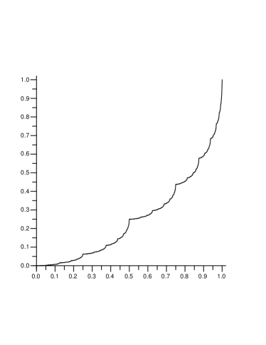
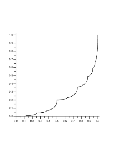
Figure 1. Limit probability distributions which come from a Bernoulli process described in Ex. 4.

4. Asymptotic expansion

To a linear representation $L$, $(A_{r})_{0\leq r<B}$, $C$, we associate a vector-valued sequence of running sums

$$\mathbf{S}_{K}(x)=\sum_{\begin{subarray}{c}\lvert w\rvert=K\\ (0.w)_{{B}}\leq x\end{subarray}}A_{w}C.$$

We want to derive an asymptotic expansion for the sequence $(\mathbf{S}_{K})$ and as a by-product an asymptotic expansion for the sequence $(S_{K})=(L\mathbf{S}_{K})$. Theorem A and its corollaries provide a one term expansion

$$\mathbf{S}_{K}(x)\mathop{=}_{K\to+\infty}R(K)\mathbf{F}(x)+o(R(K)).$$

In order to obtain a more precise expansion, we generalize the result of Corollary 2, which deals with eigenvectors of $Q$. We find a basis which reduces the matrix $Q=\sum_{0\leq r<B}A_{r}$ to its Jordan normal form and we decompose the column vector $C$ on this basis. The sequence $(\mathbf{S}_{K})$ appears as a sum of sequences associated to the vectors of the basis. We have to discuss according to the eigenvalue of $Q$ relative to each vector. If the modulus of an eigenvalue is larger than $\lambda_{*}$ we have to consider a generalized eigenvector or a Jordan vector and this will be made in the next section. After that it remains only to consider the case where the modulus is less or equal to the joint spectral radius $\lambda_{*}$. This case produces a noise which will enter in the error term of the asymptotic expansion.

4.1. Jordan vector

We use a family of linearly independent vectors $(V^{(j)})_{0\leq j<\nu}$ which satisfies $QV^{(j)}=\rho\omega V^{(j)}+V^{(j-1)}$ for $j>0$ and $QV^{(0)}=\rho\omega V^{(0)}$, with $\rho>\lambda_{*}$ and $|\omega|=1$, that is we assume Hypothesis 1 with Hypothesis 1. As a consequence $Q$ induces on the vector space generated by $V^{(0)}$, $V^{(1)}$, $\ldots$, $V^{(\nu-1)}$ the usual Jordan block of size $\nu$,

(9) $$J_{\rho\omega}=\left(\begin{array}[]{ccccc}\rho\omega&1&&&\\ &\rho\omega&1&&\\ &&\ddots&\ddots&\\ &&&&1\\ &&&&\rho\omega\end{array}\right).$$

This gives immediately

(10) $$Q^{K}V^{(\nu-1)}=\binom{K}{\nu-1}(\rho\omega)^{K-\nu+1}V^{(0)}+\binom{K}{\nu-2}(\rho\omega)^{K-\nu+2}V^{(1)}+\dotsb\\ +\binom{K}{1}(\rho\omega)^{K-1}V^{(\nu-2)}+(\rho\omega)^{K}V^{(\nu-1)}.$$

We claim that the running sum associated to the vector $V^{(\nu-1)}$

$$\mathbf{S}_{K}(x)=\sum_{\begin{subarray}{c}\lvert w\rvert=K\\ (0.w)_{{B}}\leq x\end{subarray}}A_{w}V^{(\nu-1)}$$

admits an asymptotic expansion of the form

$$\mathbf{S}_{K}(x)\mathop{=}_{K\to+\infty}\binom{K}{\nu-1}(\rho\omega)^{K-\nu+1}\mathbf{F}^{(0)}(x)+\binom{K}{\nu-2}(\rho\omega)^{K-\nu+2}\mathbf{F}^{(1)}(x)+\dotsb\\ +\binom{K}{1}(\rho\omega)^{K-1}\mathbf{F}^{(\nu-2)}(x)+(\rho\omega)^{K}\mathbf{F}^{(\nu-1)}(x)+\operatorname{error}_{K}(x),$$

where the $\mathbf{F}^{(j)}$’s are continuous functions from $[0,1]$ into $\mathbb{C}^{d}$ and the error term is $O(\lambda^{K})$ for every $\lambda>\lambda_{*}$.

The polynomial function $K\mapsto(\rho\omega)^{-K}Q^{K}V^{(\nu-1)}$ has a unique writing on the basis $\binom{K}{j}$, $0\leq j<\nu$, and we have necessarily $\mathbf{F}^{(j)}(1)=V^{(j)}$ for $0\leq j<\nu$. In the same manner the uniqueness of asymptotic expansions shows that the family $(\mathbf{F}^{(j)})_{0\leq j<\nu}$ must satisfy the system of dilation equations,

(11) $$\left\{\begin{array}[]{rcl}\rho\omega\mathbf{F}^{(0)}(x)&=&\displaystyle\sum_{r_{1}<x_{1}}A_{r_{1}}V^{(0)}+A_{x_{1}}\mathbf{F}^{(0)}(Bx-x_{1}),\\[12.91663pt] \mathbf{F}^{(0)}(x)+\rho\omega\mathbf{F}^{(1)}(x)&=&\displaystyle\sum_{r_{1}<x_{1}}A_{r_{1}}V^{(1)}+A_{x_{1}}\mathbf{F}^{(1)}(Bx-x_{1}),\\ &\vdots&\\ \mathbf{F}^{(\nu-2)}(x)+\rho\omega\mathbf{F}^{(\nu-1)}(x)&=&\displaystyle\sum_{r_{1}<x_{1}}A_{r_{1}}V^{(\nu-1)}+A_{x_{1}}\mathbf{F}^{(\nu-1)}(Bx-x_{1}).\end{array}\right.$$

We obtain these formulæ by substituting the asymptotic expansion into the functional equation of Lemma 1. Evidently the first equation of the system is nothing but the basic dilation equation (6). To obtain the proposition we have in mind, we will follow the same path as in Sections 3.1–3.3. For the sake of clarity we cut the proof into lemmas.

Lemma 4.

Under Hypotheses 1 and 1, System (11) has a unique solution $(\mathbf{F}^{(j)})_{0\leq j<\nu}$ in the space $\Pi_{0\leq j<\nu}\mathcal{C}^{(j)}$ where $\mathcal{C}^{(j)}$ is the space of continuous functions from $[0,1]$ into $\mathbb{C}^{d}$ which satisfy $\mathbf{F}^{(j)}(0)=0$, $\mathbf{F}^{(j)}(1)=V^{(j)}$ for $0\leq j<\nu$.

Proof.

It is possible to consider one equation at a time, but it is more enlightening to deal globally with the system. Let us introduce the matrix $\mathbb{F}(x)$ of type $d\times\left[0,\nu\right)$ whose columns are the column vectors $\mathbf{F}^{(0)}(x)$, $\mathbf{F}^{(1)}(x)$, $\ldots$, $\mathbf{F}^{(\nu-1)}(x)$. The system writes

(12) $$\mathbb{F}(x)J_{\rho\omega}=\sum_{r<x_{1}}A_{r}V+A_{x_{1}}\mathbb{F}(Bx-x_{1}),$$

where $V$ is the matrix whose columns are the column vectors $V^{(0)}$, $V^{(1)}$, $\ldots$, $V^{(\nu-1)}$, and $J_{\rho\omega}$ is the Jordan block defined by Eq. (9). Because of the positivity of $\rho$, the matrix $J_{\rho\omega}$ is invertible and the system turns out to be a fixed point equation $\mathbb{F}=\mathcal{L}\mathbb{F}$, namely

$$\mathbb{F}(x)=\sum_{r<x_{1}}A_{r}VJ_{\rho\omega}^{-1}+A_{x_{1}}\mathbb{F}(Bx-x_{1})J_{\rho\omega}^{-1}$$

for some operator $\mathcal{L}$. Let $\mu$ lie between $\lambda_{*}$ and $\rho$, that is $\lambda_{*}<\mu<\rho$. Because the spectral radius of $J_{\rho\omega}^{-1}$ is $1/\rho$, there exists an induced norm which provides $1/\rho\leq\|J_{\rho\omega}^{-1}\|<1/\mu$. Next there exists an integer $T$ which gives $\lambda_{*}\leq\lambda_{T}<\mu$. We consider for a while that the radix is $B^{T}$. From $\left\|A_{x_{1}}\right\|\|J_{\rho\omega}^{-1}\|<\mu\times 1/\mu=1$, we see that the right-hand side of the previous equation turns out to be the image of $\mathbb{F}$ by a contracting operator. We conclude as in the proof of Proposition 1 that the equation $\mathbb{F}=\mathcal{L}^{T}\mathbb{F}$ has a unique continuous solution $\mathbb{F}^{(0)}$ from $[0,1]$ into the space of matrices $\operatorname{M}_{d\times\left[0,\nu\right)}({\mathbb{C}})$ which satisfies the constraints $\mathbb{F}^{(0)}(0)=0$, $\mathbb{F}^{(0)}(1)=V$. Next we prove that $\mathbb{F}^{(0)}$ is the unique solution of the problem, in the same way we have finished the proof of Theorem A. ∎

Lemma 5.

Let $\mathbf{A}_{K}$ be the function from $[0,1]$ into $\mathbb{C}^{d}$ defined by

$$\mathbf{A}_{K}(x)=\binom{K}{\nu-1}(\rho\omega)^{K-\nu+1}\mathbf{F}^{(0)}(x)+\binom{K}{\nu-2}(\rho\omega)^{K-\nu+2}\mathbf{F}^{(1)}(x)+\dotsb\\ +\binom{K}{1}(\rho\omega)^{K-1}\mathbf{F}^{(\nu-2)}(x)+(\rho\omega)^{K}\mathbf{F}^{(\nu-1)}(x)$$

for each nonnegative integer $K$, where $\mathbf{F}^{(0)}$, $\ldots$, $\mathbf{F}^{(\nu-1)}$ are the functions whose existence and uniqueness are asserted by Lemma 4. Under Hypotheses 1 and 1, the running sum $\mathbf{S}_{K}$ associated to $V^{(\nu-1)}$ writes $\mathbf{S}_{K}(x)=\mathbf{A}_{K}(x)+O(\lambda^{K})$ for every $\lambda>\lambda_{*}$ and the big oh is uniform with respect to $x$ in $[0,1]$. Moreover if $\lambda_{*}$ is attained we may replace $\lambda$ by $\lambda_{*}$.

Proof.

With $\operatorname{error}_{K}(x)=\mathbf{S}_{K}(x)-\mathbf{A}_{K}(x)$ it is not difficult to obtain, by substitution, the recursion

$$\operatorname{error}_{K+1}(x)=A_{x_{1}}\operatorname{error}_{K}(Bx-x_{1}).$$

More precisely, we use the recursion of Lemma 1, System (11), and the fundamental formula of binomial coefficients. For $\lambda>\lambda_{*}$ we choose an integer $T$ such that $\lambda_{*}\leq\lambda_{T}<\lambda$. We readily obtain $\left\|\operatorname{error}_{KT}\right\|_{\infty}=O(\lambda_{T}^{KT})$. Next the recursion shows that we have $\left\|\operatorname{error}_{KT+s}\right\|_{\infty}=O(\lambda_{T}^{KT+s})$ for $0\leq s<T$, hence the result. If $\lambda_{*}$ is some $\lambda_{T}$, it is useless to consider a $\lambda>\lambda_{*}$. ∎

As in Lemma 3, we show that the functions $\mathbf{F}^{(j)}$’s are somewhat regular.

Lemma 6.

Under Hypotheses 1 and 1, each of the functions $\mathbf{F}^{(j)}$, $0\leq j<\nu$, defined in Lemma 4 is Hölder with exponent $\log_{B}(\rho/\lambda)$ for every $\lambda>\lambda_{*}$. If $\lambda_{*}$ is attained, they are Hölder with exponent $\log_{B}(\rho/\lambda_{*})$.

Proof.

We define a sequence of parameterized curves in the space of matrices of type $d\times\left[0,\nu\right)$. The first one is $\varGamma_{0}=0$ and the others are defined by the recursion $\varGamma_{K+1}=\mathcal{L}\varGamma_{K}$, where $\mathcal{L}$ is the operator we used in the proof of Lemma 4, namely

$$\varGamma_{K+1}(x)=\sum_{r<x_{1}}A_{r}VJ_{\rho\omega}^{-1}+A_{x_{1}}\varGamma_{K}(Bx-x_{1})J_{\rho\omega}^{-1}.$$

Each $\varGamma_{K}$ is piecewise linear.

We choose an induced norm and a $T$ such that $\lambda_{*}\leq\lambda_{T}<\rho$, and we consider that we use the radix $B^{T}$. As in the proof of Proposition 3 we observe that the sequence $(\varGamma_{KT})$ converges uniformly towards the solution $\mathbb{F}=(\mathbf{F}^{(j)})_{0\leq j<\nu}$ described in Lemma 4. This permits us to show that $\mathbb{F}$ is Hölder with exponent $\log_{B}(\rho/\lambda_{T})$. The argument remains the same: the maximal speed of a piecewise linear function is the greatest uniform speed on each piece and to compute a uniform speed it is sufficient to test two distinct points of the interval under consideration. ∎

We summarize the obtained result.

Proposition 4.

Under Hypotheses 1 and 1, System (11) has a unique solution $(\mathbf{F}^{(j)})_{0\leq j<\nu}$ in the space of continuous functions from $[0,1]$ into $\mathbb{C}^{d\times\left[0,\nu\right)}$ such that $\mathbf{F}^{(j)}(0)=0$, $\mathbf{F}^{(j)}(1)=V^{(j)}$ for $0\leq j<\nu$. Each of the functions $\mathbf{F}^{(j)}$, $0\leq j<\nu$, is Hölder with exponent $\log_{B}(\rho/\lambda)$ for every $\lambda>\lambda_{*}$. The running sum $\mathbf{S}_{K}$ associated to $V^{(\nu-1)}$ admits the asymptotic expansion

$$\mathbf{S}_{K}(x)=\binom{K}{\nu-1}(\rho\omega)^{K-\nu+1}\mathbf{F}^{(0)}(x)+\binom{K}{\nu-2}(\rho\omega)^{K-\nu+2}\mathbf{F}^{(1)}(x)+\dotsb\\ +\binom{K}{1}(\rho\omega)^{K-1}\mathbf{F}^{(\nu-2)}(x)+(\rho\omega)^{K}\mathbf{F}^{(\nu-1)}(x)+O(\lambda^{K})$$

for every $\lambda>\lambda_{*}$ and the big oh is uniform with respect to $x$ in $[0,1]$. Moreover if $\lambda_{*}$ is attained, the functions $\mathbf{F}^{(j)}$’s, $0\leq j<\nu$, are Hölder with exponent $\log_{B}(\rho/\lambda_{*})$, and we may replace $\lambda$ by $\lambda_{*}$ in the asymptotic expansion.

Despite of its technical aspect, the obtained result is very simple: each term of the expansion of $Q^{K}V^{(\nu-1)}$ is shaken by a somewhat regular vector-valued function which goes from $0$ to the vector which appears at the same place in the expansion.

4.2. Noise

So far we did not take into account the case $\rho\leq\lambda_{*}$. Some experiments lead us to expect a chaotic behaviour for the running sums and we content ourselves with exhibiting a natural bound.

First we consider an eigenvector $V$ of $Q$ associated to an eigenvalue $\rho\omega$, with $\rho\geq 0$ and $|\omega|=1$. Note that this time the modulus $\rho$ may be $0$.

Lemma 7.

Let $V$ be an eigenvector for $Q$ with eigenvalue of modulus $\rho\geq 0$ which satisfies $\rho\leq\lambda_{*}$. The sequence of running sums associated to $V$ satisfies $\left\|\mathbf{S}_{K}\right\|_{\infty}=O(\lambda^{K})$ for every $\lambda>\lambda_{*}$. If $\lambda_{*}$ is attained, we may replace $O(\lambda^{K})$ by $O(\lambda_{*}^{K})$ in case $\rho<\lambda_{*}$ and by $O(K\lambda_{*}^{K})$ in case $\rho=\lambda_{*}$.

Proof.

The functional equation satisfied by the running sum associated to the eigenvector $V$ is

$$\mathbf{S}_{K+1}(x)=\sum_{r_{1}<x_{1}}A_{r_{1}}Q^{K}V+A_{x_{1}}\mathbf{S}_{K}(Bx-x_{1}),$$

that is

$$\mathbf{S}_{K+1}(x)=(\rho\omega)^{K}\sum_{r_{1}<x_{1}}A_{r_{1}}V+A_{x_{1}}\mathbf{S}_{K}(Bx-x_{1}).$$

Let us assume first that we have a $\lambda$ such that $\rho\leq\lambda$ and $\left\|A_{r}\right\|\leq\lambda$ for $0\leq r<B$ and for some induced norm, that is let us assume in a certain sense the converse of Hypothesis 1. We obtain

$$\left\|\mathbf{S}_{K+1}(x)\right\|\leq\rho^{K}\sum_{r_{1}<x_{1}}\lambda\left\|V\right\|+\lambda\left\|\mathbf{S}_{K}(Bx-x_{1})\right\|,$$

hence

$$\left\|\mathbf{S}_{K+1}\right\|_{\infty}\leq\rho^{K}B\lambda\left\|V\right\|+\lambda\left\|\mathbf{S}_{K}\right\|_{\infty}.$$

With $\left\|\mathbf{S}_{K}\right\|_{\infty}=\lambda^{K}u_{K}$, we have $u_{K+1}\leq(\rho/\lambda)^{K}B\left\|V\right\|+u_{K}$. In case $\rho<\lambda$, we have $u_{K}\leq u_{0}+B\left\|V\right\|/(1-\rho/\lambda)$ and we conclude $\left\|\mathbf{S}_{K}\right\|_{\infty}=O(\lambda^{K})$. In case $\rho=\lambda$, we have $u_{K}\leq u_{0}+KB\left\|V\right\|$ and we conclude $\left\|\mathbf{S}_{K}\right\|_{\infty}=O(K\lambda^{K})$.

Second we consider the general case, which divides into two sub-cases. Let us assume that the joint spectral radius is smaller that all $\lambda_{T}$, for every induced norm. For any $\lambda>\lambda_{*}$, we may find, for a given induced norm, a $T$ such that $\lambda_{*}<\lambda_{T}\leq\lambda$. We apply the previous argument to the sequence $(\mathbf{S}_{KT})$. This gives $\left\|\mathbf{S}_{KT}\right\|_{\infty}=O(\lambda_{T}^{KT})$ because we have $\rho\leq\lambda_{*}<\lambda_{T}$. Next, Lemma 1 gives $\left\|\mathbf{S}_{KT+s}\right\|_{\infty}=O(\lambda_{T}^{KT+s})$ for $0\leq s<T$, because there is a finite number of $s$ between $0$ and $T$. In this way, we obtain $\left\|\mathbf{S}_{K}\right\|_{\infty}=O(\lambda_{T}^{K})$, and we conclude $\left\|\mathbf{S}_{K}\right\|_{\infty}=O(\lambda^{K})$ for every $\lambda>\lambda_{*}$.

Let us assume that $\lambda_{*}$ is some $\lambda_{T}$ for some induced norm. In case $0\leq\rho<\lambda_{*}=\lambda_{T}$ the same reasoning as above, with $\lambda_{*}$ in place of $\lambda$, gives $\left\|\mathbf{S}_{K}\right\|_{\infty}=O(\lambda_{*}^{K})$. In case $\rho=\lambda_{*}$ we find $\left\|\mathbf{S}_{KT}\right\|_{\infty}=O(K\lambda_{*}^{KT})$. As above and again because there is a finite number of integers between 0 and $T$, we obtain $\left\|\mathbf{S}_{K}\right\|_{\infty}=O(K\lambda_{*}^{K})$. ∎

The next example shows that the upper bound we have found in case $\rho=\lambda_{*}$ has the right order of growth.

Example 5 [Triangular tiling].

For a real $\vartheta$, we consider the rotation matrix

$$R_{\vartheta}=\left(\begin{array}[]{cc}\cos{\vartheta}&-\sin{\vartheta}\\ \sin{\vartheta}&\cos{\vartheta}\end{array}\right).$$

In the following we use $V_{0}=E_{1}$ the first vector of the canonical basis and $V_{\vartheta}=R_{\vartheta}V_{0}$. The example is based on the linear representation

$$L=\left(\begin{array}[]{cc}1&0\end{array}\right),\qquad A_{0}=R_{-\vartheta},\qquad A_{1}=R_{\vartheta},\qquad C=V_{0}.$$

Because we use orthogonal matrices, the joint spectral radius is $\lambda_{*}=1$. We specialize the case to $\vartheta=\pi/3$, so that we have $\rho=\lambda_{*}$.

We consider the words $u=11$, $v=01$, and the rational numbers $x_{2K+2}$ and $y_{2K}$ whose binary expansions are $(0.uv^{K})_{2}$ and $(0.v^{K})_{2}$ respectively. According to the functional equation satisfied by $(\mathbf{S}_{K})$, we have

$$\mathbf{S}_{2K+2}(x_{2K+2})=R_{-{\pi/3}}V_{0}+R_{{\pi/3}}\left(R_{-{\pi/3}}V_{0}+R_{{\pi/3}}S_{2K}(y_{2K})\right)\\ =V_{-{\pi/3}}+V_{0}+R_{2{\pi/3}}S_{2K}(y_{2K}),$$

$$\mathbf{S}_{2K}(y_{2K})=R_{-{\pi/3}}\left(R_{-{\pi/3}}V_{0}+R_{{\pi/3}}\mathbf{S}_{2K-2}(y_{2K-2})\right)=V_{-2{\pi/3}}+\mathbf{S}_{2K-2}(y_{2K-2}).$$

With $\mathbf{S}_{0}(\varepsilon)=V_{0}$ ($\varepsilon$ is the empty word), we obtain by induction $\mathbf{S}_{2K}(y_{2K})=KV_{-2{\pi/3}}+V_{0}$ and

$$\mathbf{S}_{2K+2}(x_{2K+2})=(K+1)V_{0}+V_{-{\pi/3}}+V_{2{\pi/3}}=(K+1)V_{0}.$$

Hence the $O(K\lambda_{*}^{K})$ we have found in Lemma 7 is satisfying.

The orbit of the parameterized curve $\mathbf{S}_{K}$ is illustrated in Fig. 2. In this example the recurrences which define the sequence $(\mathbf{S}_{K})$ and the sequence $(\mathbf{F}_{K})$ are exactly the same. Moreover computing the values $\mathbf{S}_{K}(x)$ for a rational $x$ whose binary expansion has length at most $K$ is almost the same as computing the values $\mathbf{F}(x)$ for a hypothetical solution of the basic dilation equation. This is not really true because $A_{0}V_{0}$ is not $V_{0}$, and the less significant bits with value $0$ must be taken into account. (Look at Fig. 2. From the first to the second picture a half-turn has been applied to the little pattern of the leftmost picture, because $A_{0}^{3}=-\operatorname{I}_{2}$.) But $A_{0}^{6}=\operatorname{I}_{2}$ and if we use radix $2^{6}=64$ in place of $2$ this problem disappears. The computation we have made shows that the basic dilation equation has no solution: if $\mathbf{F}$ was a solution, it would satisfy $\mathbf{F}(y)=V_{-2{\pi/3}}+\mathbf{F}(y)$ for $y=1/3=(0.010101\ldots)_{2}$.

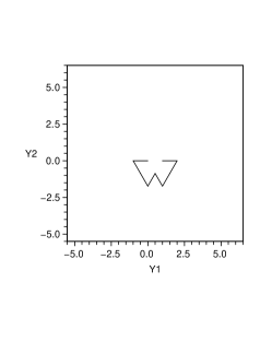
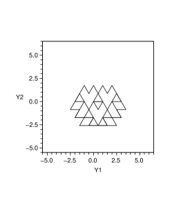
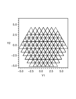
Figure 2. The image of the parameterized curve $\mathbf{S}_{K}$ from Ex. 5 grows linearly with $K$. Here we see $\mathbf{S}_{3}$, $\mathbf{S}_{6}$, and $\mathbf{S}_{12}$.

We generalize slightly the previous lemma into the following assertion.

Proposition 5.

Under Hypothesis 1 with $0\leq\rho\leq\lambda_{*}$, the sequence of running sums $(\mathbf{S}_{K})$ associated to $V^{(\nu-1)}$ satisfies $\left\|\mathbf{S}_{K}\right\|_{\infty}=O(\lambda^{K})$ for every $\lambda>\lambda_{*}$. Moreover if $\lambda_{*}$ is attained, we may replace $O(\lambda^{K})$ by $O(\lambda_{*}^{K})$ in case $\rho<\lambda_{*}$ and by $O(\lambda_{*}^{K}K^{\nu})$ otherwise.

Proof.

The generalized eigenvector $V^{(\nu-1)}$ satisfies $Q^{K}V^{(\nu-1)}=O(\rho^{K}K^{\nu-1})$. As above we conclude $\left\|\mathbf{S}_{K}\right\|_{\infty}=O(\lambda^{K})$ for every $\lambda>\lambda_{*}$. We may refine the computation in case $\lambda_{*}$ is some $\lambda_{T}$ : in that case, if $\rho<\lambda_{*}$ we have $\left\|\mathbf{S}_{K}\right\|_{\infty}=O(\lambda_{*}^{K})$, and if $\rho=\lambda_{*}$ we obtain $\left\|\mathbf{S}_{K}\right\|_{\infty}=O(\lambda_{*}^{K}K^{\nu})$. ∎

Example 6 [Powers of $2$ characteristic sequence].

The sequence $(u(n))$ which takes value $1$ on the powers of $2$ and $0$ on the others integers admits the generating family $(u(n),u(2n+1))$ and the linear representation

$$L=\left(\begin{array}[]{cc}0&1\end{array}\right),\qquad A_{0}=\left(\begin{array}[]{cc}1&0\\ 0&1\end{array}\right),\qquad A_{1}=\left(\begin{array}[]{cc}0&0\\ 1&0\end{array}\right),\qquad C=\left(\begin{array}[]{c}1\\ 0\end{array}\right).$$

Matrix $Q=A_{0}+A_{1}$ has $1$ as a unique eigenvalue and the plane $\mathbb{R}^{2}$ is the characteristic subspace $\operatorname{Ker}(Q-\operatorname{I}_{2})^{2}$. Hypothesis 1 is satisfied with

$$\rho=1,\qquad R(K)=K,\qquad V=\left(\begin{array}[]{cc}0&1\end{array}\right)^{{\mathrm{tr}}}.$$

The joint spectral radius is $\lambda_{*}=1$ (consider $A_{0}$). The fixed point equation is

$$\left\{\begin{array}[]{l}F_{1}(x)=F_{1}(2x),\\ F_{2}(x)=F_{2}(2x),\end{array}\right.\quad\text{for $0\leq x<\frac{1}{2}$\,;}\qquad\left\{\begin{array}[]{l}F_{1}(x)=0,\\ F_{2}(x)=1+F_{1}(2x-1),\end{array}\right.\quad\text{for $\frac{1}{2}\leq x<1$.}$$

It admits the only solution (consider $F_{1}$ and first the interval $\left[1/2,1\right[$, next the interval $\left[1/4,1/2\right[$, and so on)

$$\mathbf{F}(x)=\left\{\begin{array}[]{ll}(\begin{array}[]{cc}0&1\end{array})^{{\mathrm{tr}}}&\text{if $0<x\leq 1$,}\\ (\begin{array}[]{cc}0&0\end{array})^{{\mathrm{tr}}}&\text{if $x=0$.}\end{array}\right.$$

(We do not forget the conditions $\mathbf{F}(0)=0$, $\mathbf{F}(1)=V$.) The sequence $(\mathbf{F}_{K})$ satisfies

$$\mathbf{F}_{K}(x)=\left\{\begin{array}[]{ll}(\begin{array}[]{cc}0&0\end{array})^{{\mathrm{tr}}}&\text{if $0\leq x<1/2^{K}$,}\\ (\begin{array}[]{cc}1/K&k/K\end{array})^{{\mathrm{tr}}}&\text{if $2^{k-1}/2^{K}\leq x<2^{k}/2^{K}$ for $1\leq k\leq K$,}\\ (\begin{array}[]{cc}1/K&1\end{array})^{{\mathrm{tr}}}&\text{if $x=1.$}\end{array}\right.$$

It turns out that $(\mathbf{F}_{K})$ converges simply towards $\mathbf{F}$. This implies that we have $\mathbf{S}_{K}(x)=K\mathbf{F}(x)+O(1)$ and $\left\|\mathbf{S}_{K}\right\|_{\infty}\sim K$.

Previous Examples 5 and 6 show that under the condition $\rho=\lambda_{*}$ the sequence of running sums $(\mathbf{S}_{K})$ can or cannot define a limit function $\mathbf{F}$ according to the case.

4.3. General case

The general case is obtained by expanding the vector $C$ over a Jordan basis for $Q$. Let us recall that the height of a generalized eigenvector is the dimension of the subspace it spans under the action of $Q$. Gathering Prop. 4 and 5, we arrive at the following assertion.

Theorem B.

Let $L$, $(A_{r})_{0\leq r<B}$, $C$ be a linear representation of a rational formal power series. The sequence of running sums

$$\mathbf{S}_{K}(x)=\sum_{\begin{subarray}{c}\lvert w\rvert=K\\ (0.w)_{{B}}\leq x\end{subarray}}A_{w}C$$

admits an asymptotic expansion with error term $O(\lambda^{K})$ for every $\lambda>\lambda_{*}$, where $\lambda_{*}$ is the joint spectral radius of the family $(A_{r})_{0\leq r<B}$. The used asymptotic scale is the family of sequences $\rho^{K}\binom{K}{\ell}$, $\rho>0$, $\ell\in\mathbb{N}_{\geq 0}$. The error term is uniform with respect to $x\in[0,1]$.

If $C$ is a generalized eigenvector $V$ for $Q$ of height $\nu$ associated to an eigenvalue $\rho\omega$ of modulus $\rho>\lambda_{*}$ and if $(V^{(j)})_{0\leq j<\nu}$ is the associated family of vectors such that $V^{(\nu-1)}=V$, $QV^{(j)}=\rho\omega V^{(j)}+V^{(j-1)}$ for $j>0$ and $QV^{(0)}=\rho\omega V^{(0)}$ , from the expansion

$$Q^{K}V=\binom{K}{\nu-1}(\rho\omega)^{K-\nu+1}V^{(0)}+\binom{K}{\nu-2}(\rho\omega)^{K-\nu+2}V^{(1)}+\dotsb\\ +\binom{K}{1}(\rho\omega)^{K-1}V^{(\nu-2)}+(\rho\omega)^{K}V^{(\nu-1)}.$$

is deduced the asymptotic expansion

$$\sum_{\begin{subarray}{c}\lvert w\rvert=K\\ (0.w)_{{B}}\leq x\end{subarray}}A_{w}V\mathop{=}_{K\to+\infty}\binom{K}{\nu-1}(\rho\omega)^{K-\nu+1}\mathbf{F}^{(0)}(x)+\binom{K}{\nu-2}(\rho\omega)^{K-\nu+2}\mathbf{F}^{(1)}(x)\\ +\dotsb+\binom{K}{1}(\rho\omega)^{K-1}\mathbf{F}^{(\nu-2)}(x)+(\rho\omega)^{K}\mathbf{F}^{(\nu-1)}(x)+O(\lambda^{K})$$

where the family $(\mathbf{F}^{(j)})_{0\leq j<\nu}$ is the unique solution to the system of dilation equations

$$\left\{\begin{array}[]{rcl}\rho\omega\mathbf{F}^{(0)}(x)&=&\displaystyle\sum_{r_{1}<x_{1}}A_{r_{1}}V^{(0)}+A_{x_{1}}\mathbf{F}^{(0)}(Bx-x_{1}),\\[12.91663pt] \mathbf{F}^{(0)}(x)+\rho\omega\mathbf{F}^{(1)}(x)&=&\displaystyle\sum_{r_{1}<x_{1}}A_{r_{1}}V^{(1)}+A_{x_{1}}\mathbf{F}^{(1)}(Bx-x_{1}),\\ &\vdots&\\ \mathbf{F}^{(\nu-2)}(x)+\rho\omega\mathbf{F}^{(\nu-1)}(x)&=&\displaystyle\sum_{r_{1}<x_{1}}A_{r_{1}}V^{(\nu-1)}+A_{x_{1}}\mathbf{F}^{(\nu-1)}(Bx-x_{1}).\end{array}\right.$$

Moreover if the joint spectral radius $\lambda_{*}$ is attained, the error term may be improved in the following way. Let $\mathcal{V}$ be a Jordan basis for  $Q$. Let $m$ be the maximal height of the generalized eigenvectors $V$ from $\mathcal{V}$ associated to an eigenvalue of modulus $\lambda_{*}$ such that the vector $C$ has a nonzero component over $V$, with $m=0$ if there does not exist such generalized eigenvector. The error term may be taken as $O(\lambda_{*}^{K}K^{m})$.

The asymptotic expansion is concretely obtained by the algorithm of page 1 named LRtoAE1 (for linear representation to asymptotic expansion). Clearly this gives an asymptotic expansion for the number-valued sum $S_{K}(x)=L\mathbf{S}_{K}(x)$ too. It is noteworthy that two important hypotheses are made in the algorithm. First it is assumed that the joint spectral radius $\lambda_{*}$ is known and even more it is assumed that we know if the joint spectral radius is attained. This is not an obstacle to the use of the algorithm. If we have at our disposal an upper bound $\lambda_{+}>\lambda_{*}$, we may replace $\lambda_{*}$ by $\lambda_{+}$, obtaining of course a less precise expansion. Second it is assumed that we can solve dilation equations according to Lemma 4. This is evidently wrong in full generality, but the solution is mathematically well defined and may be computed exactly over a dense subset by the cascade algorithm.

Input : A linear representation $L$, $(A_{r})_{0\leq r<B}$, $C$, and its joint spectral radius $\lambda_{*}$.

Output : An asymptotic expansion of the running sum $\mathbf{S}_{K}(x)$ associated to the vector $C$ when $K$ goes to infinity at the precision ${O\tilde{\phantom{\imath}}}(\lambda_{*}^{K})$ if $\lambda_{*}$ is attained and $O(\lambda^{K})$ for a $\lambda$ slightly greater than $\lambda_{*}$ if not, with respect to the scale $\rho^{K}\binom{K}{\ell}$, $\rho>0$, $\ell\in\mathbb{N}_{\geq 0}$.

$Q:=\sum_{0\leq r<B}A_{r}$;AlgoLine0.1

if $\lambda_{*}$ is attained then  $\lambda:=\lambda_{*}$ else  $\lambda:=$ any number between $\lambda_{*}$ and the infimum of the modulus of eigenvalues of $Q$ greater than $\lambda_{*}$ end compute a Jordan basis $\mathcal{V}$ for the matrix $Q$;AlgoLine0.2

expand the column vector $C$ of the linear representation over the Jordan basis, as $C=\sum_{V\in\mathcal{V}}\gamma_{V}V$;AlgoLine0.3

$\mathcal{V}_{>}:=$ the set of generalized eigenvectors in $\mathcal{V}$ such that $\gamma_{V}\neq 0$ and the associated eigenvalue $\rho\omega$ has a modulus $\rho>\lambda$;AlgoLine0.4

for each vector $V$ in $\mathcal{V}_{>}$ do  $\rho\omega:=$ the eigenvalue associated to $V$; AlgoLine0.5

$\nu:=$ the height of $V$;AlgoLine0.6

an asymptotic expansion

$$\mathbf{A}_{V;K}(x):=\binom{K}{\nu-1}(\rho\omega)^{K-\nu+1}\mathbf{F}^{(0)}(x)+\binom{K}{\nu-2}(\rho\omega)^{K-\nu+2}\mathbf{F}^{(1)}(x)+\mbox{}\\ \dotsb+\binom{K}{1}(\rho\omega)^{K-1}\mathbf{F}^{(\nu-2)}(x)+(\rho\omega)^{K}\mathbf{F}^{(\nu-1)}(x)\qquad$$

is deduced from Proposition 4end $\mathbf{A}_{K}(x):=\sum_{V\in\mathcal{V}_{>}}\gamma_{V}\mathbf{A}_{V;K}(x)$;AlgoLine0.7

$\operatorname{error~{}term}_{K}(x):=O(\lambda^{K})$;AlgoLine0.8

if $\lambda_{*}$ is attained then  $\mathcal{V}_{=}:=$ the set of generalized eigenvectors in $\mathcal{V}$ such that $\gamma_{V}\neq 0$ and the associated eigenvalue $\rho\omega$ has a modulus $\rho=\lambda_{*}$; AlgoLine0.9

$m:=0$;AlgoLine0.10

for each $V$ in $\mathcal{V}_{=}$ do  $\nu:=$ the height of $V$; AlgoLine0.11

$m:=\max(m,\nu)$end $\operatorname{error~{}term}_{K}(x):=O(\lambda_{*}^{K}K^{m})$end return

$$\mathbf{S}_{K}(x)\mathop{=}_{K\to+\infty}\mathbf{A}_{K}(x)+\operatorname{error~{}term}_{K}(x)$$

Algorithm 1 LRtoAE1

11

11

11

11

11

11

11

11

11

11

11

Example 7 [Lipmaa–Wallen’s formal power series].

For a nonnegative integer $K$, the ring ${\mathbb{Z}}/2^{K}{\mathbb{Z}}$ may be equipped with two additions. The first one is the quotient addition $+$ which comes form the addition of the ring of integers $\mathbb{Z}$. The second one uses the identification of the set ${\mathbb{Z}}/2^{K}{\mathbb{Z}}$ with the set $({\mathbb{Z}}/2{\mathbb{Z}})^{K}$ through the correspondence which maps a $K$-tuple of bits $(\varepsilon_{k})_{0\leq k<K}$ onto the integer $\varepsilon_{0}+2\varepsilon_{1}+\dotsb+2^{K-1}\varepsilon_{K-1}$. It is the bitwise addition $\oplus$, or exclusive-or. The cryptanalysts Lipmaa and Wallen have studied the propagation of differences (in the sense of $+$) through $\oplus$ and more precisely the additive differential probability $\operatorname{adp}$ which maps a triple $(\alpha,\beta,\gamma)\in({\mathbb{Z}}/2^{K}{\mathbb{Z}})^{3}$ onto the probability that the difference $((x+\alpha)\oplus(y+\beta))-x\oplus y$ has value $\gamma$ for $x$, $y$ taken from ${\mathbb{Z}}/2^{K}{\mathbb{Z}}$ with equiprobability. By coding every triple $(\alpha,\beta,\gamma)$ as a word $w$ over the alphabet ${\mathbb{Z}}/8{\mathbb{Z}}$ (with $w_{k}=4\alpha_{k}+2\beta_{k}+\gamma_{k}$ for $0\leq k<K$), Lipmaa et al. (2004) show that $\operatorname{adp}$ turns out to be a rational series. With $(E_{j})_{1\leq j\leq 8}$ the canonical basis of $\mathbb{Q}^{8}$, it admits the $8$-dimensional linear representation

$$L=\sum_{0\leq r<8}E_{i}^{{\mathrm{tr}}},\qquad(A_{r})_{0\leq r<8},\qquad C=E_{1}$$

where $A_{0}$ is defined as

$$A_{0}=\frac{1}{4}\left(\begin{array}[]{cccccccc}4&0&0&1&0&1&1&0\\ 0&0&0&1&0&1&0&0\\ 0&0&0&1&0&0&1&0\\ 0&0&0&1&0&0&0&0\\ 0&0&0&0&0&1&1&0\\ 0&0&0&0&0&1&0&0\\ 0&0&0&0&0&0&1&0\\ 0&0&0&0&0&0&0&0\end{array}\right).$$

and the other matrices $A_{r}$ with $r\neq 0$ are obtained from $A_{0}$ by permuting row $i$ with row $i\oplus r$ and column $j$ with column $j\oplus r$. Using the maximum absolute column sum norm, we find $\lambda_{*}\leq 1$ and because $1$ is an eigenvalue for all matrices $A_{r}$, $0\leq r<8$, we have $\lambda_{*}=1$.

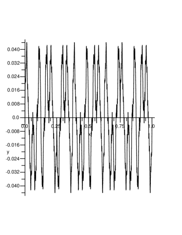
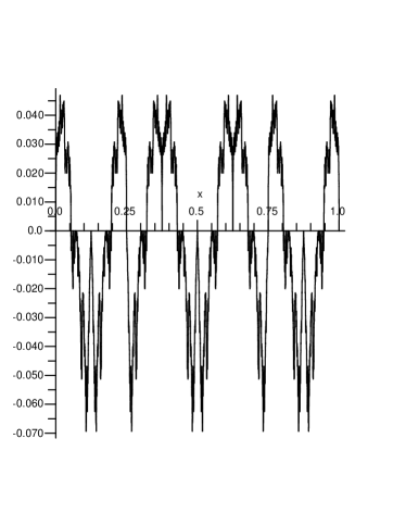
Figure 3. Refinement functions which originate from cryptanalysis (Ex. 7).

The matrix

$$Q=A_{0}+A_{1}+\dotsb+A_{7}=\frac{1}{4}\left(\begin{array}[]{cccccccc}7&2&2&1&2&1&1&0\\ 2&7&1&2&1&2&0&1\\ 2&1&7&2&1&0&2&1\\ 1&2&2&7&0&1&1&2\\ 2&1&1&0&7&2&2&1\\ 1&2&0&1&2&7&1&2\\ 1&0&2&1&2&1&7&2\\ 0&1&1&2&1&2&2&7\end{array}\right)$$

is diagonalizable, with eigenvalues $4$, $2$, $1$, and eigenspaces respectively of dimension $1$, $3$, $4$. The vector $C=E_{1}$ decomposes as $C=V_{4}+V_{2}+V_{1}$, where

$$V_{4}=\frac{1}{8}\left(\begin{array}[]{c}1\\ 1\\ 1\\ 1\\ 1\\ 1\\ 1\\ 1\end{array}\right),\qquad V_{2}=\frac{1}{8}\left(\begin{array}[]{c}3\\ 1\\ 1\\ -1\\ 1\\ -1\\ -1\\ -3\end{array}\right),\qquad V_{1}=\frac{1}{4}\left(\begin{array}[]{c}2\\ -1\\ -1\\ 0\\ -1\\ 0\\ 0\\ 1\end{array}\right)$$

are respectively eigenvectors for the eigenvalues $4$, $2$, $1$. According to Theorem B, we obtain the following asymptotic expansion (with $F_{\rho}=L\mathbf{F}_{\rho}$ for $\rho=4$, $2$)

$$\sum_{\begin{subarray}{c}\lvert w\rvert=K\\ (0.w)_{{8}}\leq x\end{subarray}}\operatorname{adp}(w)\mathop{=}_{K\to+\infty}4^{K}F_{4}(x)+2^{K}F_{2}(x)+O(K),$$

where the functions $\mathbf{F}_{4}$ and $\mathbf{F}_{2}$ are determined by the dilation equation (as usual $x_{1}$ is the first octal digits after the octal point of $x\in\left[0,1\right)$)

$$\mathbf{F}_{\rho}(x)=\frac{1}{\rho}\sum_{r<x_{1}}A_{r}V_{\rho}+\frac{1}{\rho}A_{x_{1}}\mathbf{F}_{\rho}(8x-x_{1}),\qquad\text{with $\mathbf{F}_{\rho}(0)=0$ and $\mathbf{F}_{\rho}(1)=V_{\rho}$}$$

for $\rho=4$, $2$. Functions $\mathbf{F}_{4}$ and $\mathbf{F}_{2}$ are respectively Hölder with exponent $\log_{8}4=2/3$ and $\log_{8}2=1/3$. Function $F_{4}=L\mathbf{F}_{4}$ is very near the identity and the graph of $x\mapsto F_{4}(x)-x$ is drawn on the left of Fig. 3. On the right is the graph of $F_{2}=L\mathbf{F}_{2}$. Both functions have an amplitude of order about $0.05$. The obtained result improves (Dumas et al., 2007) which gives only an error term $O(2^{K})$.

5. Radix-rational sequences and periodic functions

It is usual that sequences rational with respect to a radix introduce periodic functions in logarithmic scale. These periodic functions appear either by subtle elementary arguments, like explicit expression of the sequence with fractional part of a logarithm in base $B$, or by sophisticated argument which express partial sums by contour integral of a meromorphic function whose poles are regularly spaced on a vertical line. With the approach used in this paper, the introduction of periodic functions is natural. Nevertheless these functions are generally only pseudo-periodic functions and we will see why they are periodic in the previous works on the subject.

5.1. Asymptotic expansion

To a rational series $S$ defined by a linear representation $L$, $A_{0}$, $\ldots$, $A_{B-1}$, $C$ is associated a sequence $u$ defined in the following way: we write the integer $n$ with respect to the radix $B$, $n=(w)_{{B}}$, and the value of the sequence for $n$ is the value of the rational series for the word $w$, that is $u(n)=(S,w)$. We want to evaluate the partial sums $\sum_{0\leq n\leq N}u(n)$ of the sequence for $N$ large. With $t\in\left[0,1\right)$ and $K$ integer, we may write $N=B^{K+t}$, that is $K$ is the integer part of $\log_{B}N$ and $t$ is its fractional part. The partial sum up to $N$ is the sum of the partial sum up to $B^{K}-1$ and a complementary term. The first appears as the sum of $(S,w)$ over all words $w$ of length not greater than $K$ minus the sum over all the previous words which begin with a $0$. The complementary term appears as the running sum associated to $S$ we have studied, but without the words of length $K+1$ which begin by a $0$. This remark gives the following formula

$$\sum_{n\leq B^{K+t}}u(n)=\sum_{0\leq k\leq K}\biggl{(}\sum_{\lvert w\rvert=k}LA_{w}C-\sum_{\lvert w^{\prime}\rvert=k-1}LA_{0}A_{w^{\prime}}C\biggr{)}\\ +\biggl{(}\sum_{\begin{subarray}{c}\lvert w\rvert=K+1\\ (w)_{{B}}\leq B^{K+1}B^{t-1}\end{subarray}}LA_{w}C-\sum_{\lvert w^{\prime}\rvert=K}LA_{0}A_{w^{\prime}}C\biggr{)}$$

that is

(13) $$\sum_{n\leq B^{K+t}}u(n)=L(\operatorname{I}_{d}-A_{0})\sum_{0\leq k\leq K}Q^{k}C+\sum_{\begin{subarray}{c}\lvert w\rvert=K+1\\ (w)_{{B}}\leq B^{K+1}B^{t-1}\end{subarray}}LA_{w}C.$$

Just as we have considered the sums $\mathbf{S}_{K}(x)$, we introduce the vector-valued sums

(14) $${\mathbf{\Sigma}}_{N}=\sum_{(w)_{B}\leq N}A_{w}C,$$

that is

(15) $${\mathbf{\Sigma}}_{N}=(\operatorname{I}_{d}-A_{0})\sum_{0\leq k\leq K}Q^{k}C+\sum_{\begin{subarray}{c}\lvert w\rvert=K+1\\ (w)_{{B}}\leq B^{K+1}B^{t-1}\end{subarray}}A_{w}C$$

with $N=B^{K+t}$, $0\leq t<1$. As in the previous section, we decompose the column vector $C$ over a Jordan basis for the matrix $Q$. Hence we consider for the rest of the section a family of linearly independent vectors $(V^{(j)})_{0\leq j<\nu}$ which satisfies $QV^{(j)}=\rho\omega V^{(j)}+V^{(j-1)}$ for $j>0$ and $QV^{(0)}=\rho\omega V^{(0)}$, with $\rho>\lambda_{*}$ and $|\omega|=1$. In other words, we assume Hypotheses 1 and 1. We want to determine an asymptotic expansion for the running sums ${\mathbf{\Sigma}}_{N}$ associated to $V=V^{(\nu-1)}$.

Formula (15) expresses the running sums of the sequence as the sum of two terms. For the first term in the right member of Formula (15), we use formulæ like Eq. (10) and the following elementary summation formula

(16) $$\sum_{k=\ell}^{K}\binom{k}{\ell}\alpha^{k-\ell}=\left\{\begin{array}[]{ll}\displaystyle\binom{K}{\ell+1}+\binom{K}{\ell}&\begin{array}[]{l}\text{if $\alpha=1$,}\end{array}\\[8.61108pt] \begin{aligned} \displaystyle\binom{K}{\ell}\frac{\alpha^{K-\ell+1}}{\alpha-1}+\sum_{j=1}^{\ell}(-1)^{j}\binom{K}{\ell-j}\frac{\alpha^{K-\ell+j}}{(\alpha-1)^{j+1}}&\\ \displaystyle\mbox{}+(-1)^{\ell+1}\frac{1}{(\alpha-1)^{\ell+1}}&\end{aligned}&\begin{array}[]{l}\phantom{\displaystyle\sum_{j=1}^{\ell}}\\ \text{if $\alpha\neq 1$.}\end{array}\end{array}\right.$$

As a consequence, the first term of Formula (15) has an asymptotic expansion in the asymptotic scale $\rho^{K}\binom{K}{\ell}$, $\rho>0$, $\ell\in{\mathbb{N}}_{\geq 0}$.

Lemma 8.

Under Hypothesis 1 with $C=V^{(\nu-1)}$ the first term in the right member of Formula (15) has the following expansion

(17) $$(\operatorname{I}_{d}-A_{0})\sum_{k=0}^{K}Q^{k}V^{(\nu-1)}=\binom{K}{\nu-1}\frac{(\rho\omega)^{K-\nu+2}}{\rho\omega-1}(\operatorname{I}_{d}-A_{0})V^{(0)}\\ +\sum_{\ell=0}^{\nu-2}\binom{K}{\ell}(\rho\omega)^{K-\ell}\left[\frac{\rho\omega}{\rho\omega-1}(\operatorname{I}_{d}-A_{0})V^{(\nu-\ell-1)}\phantom{\sum_{j=\ell+1}^{\nu-1}}\right.\\ \left.+\sum_{j=\ell+1}^{\nu-1}\frac{(-1)^{j-\ell}}{(\rho\omega-1)^{j-\ell+1}}(\operatorname{I}_{d}-A_{0})V^{(\nu-j-1)}\right]\\ +\sum_{\ell=0}^{\nu-1}(-1)^{\ell+1}\frac{1}{(\rho\omega-1)^{\ell+1}}(\operatorname{I}_{d}-A_{0})V^{(\nu-\ell-1)}$$

in case $\rho\omega\neq 1$ and

(18) $$(\operatorname{I}_{d}-A_{0})\sum_{k=0}^{K}Q^{k}V^{(\nu-1)}=\binom{K}{\nu}(\operatorname{I}_{d}-A_{0})V^{(0)}\\ +\sum_{\ell=1}^{\nu-1}\binom{K}{\ell}(\operatorname{I}_{d}-A_{0})\left[V^{(\nu-\ell)}+V^{(\nu-\ell-1}\right]+(\operatorname{I}_{d}-A_{0})V^{(\nu-1)}$$

in case $\rho\omega=1$.

The previous expansion is not an asymptotic expansion but it may easily converted into such an expansion in the scale $\rho^{K}\binom{K}{\ell}$, $\rho>0$, $\ell\in\mathbb{N}_{\geq 0}$, with $K=\lfloor\log_{B}N\rfloor$. The error term depends on the relative places of $\lambda_{*}$, $\rho$, and $1$. We will return on this point in a while.

The second term in the right member of Formula (15) is nothing but $\mathbf{S}_{K+1}(B^{t-1})$. Proposition 4 translates into the following result.

Lemma 9.

Under Hypotheses 1 and 1, the second term in the right member of Formula (15) for the running sum associated to $V^{(\nu-1)}$ admits the following asymptotic expansion with respect to the scale $\rho^{K}\binom{K}{\ell}$, $\rho>0$, $\ell\in\mathbb{N}_{\geq 0}$, with $K=\lfloor\log_{B}N\rfloor$, where the functions $\mathbf{F}^{(\ell)}$’s are defined in Lemma 4,

(19) $$\sum_{\begin{subarray}{c}\lvert w\rvert=K+1\\ (w)_{{B}}\leq B^{K+1}B^{t-1}\end{subarray}}A_{w}V^{(\nu-1)}\mathop{=}_{N\to+\infty}\binom{K}{\nu-1}(\rho\omega)^{K-\nu+2}\mathbf{F}^{(0)}(B^{t-1})\\ +\sum_{\ell=0}^{\nu-2}\binom{K}{\ell}(\rho\omega)^{K-\ell}\left[\rho\omega\mathbf{F}^{(\nu-\ell-1)}(B^{t-1})+\mathbf{F}^{(\nu-\ell-2)}(B^{t-1})\right]+O(\lambda^{K}).$$

for every $\lambda>\lambda_{*}$ and the big oh is uniform with respect to $t$ in $[0,1]$. Moreover if $\lambda_{*}$ is attained we may replace $\lambda$ by $\lambda_{*}$ in the asymptotic expansion.

Proof.

Proposition 4 and the fundamental formula of binomial coefficients provide the expansion of $\mathbf{S}_{K+1}(B^{t-1})$ by a mere substitution. ∎

Gathering the results of the previous discussion, we arrive at the following qualitative theorem.

Theorem C.

Let $L$, $(A_{r})_{0\leq r<B}$, $C$ be a linear representation of a radix-rational sequence $(u_{n})$. The vector-valued running sum ${\mathbf{\Sigma}}_{N}$ defined by Equation (14) admits an asymptotic expansion with error term $O(N^{\log_{B}\lambda})$ for every $\lambda>\lambda_{*}$, where $\lambda_{*}$ is the joint spectral radius of the family $(A_{r})_{0\leq r<B}$. If $\lambda_{*}$ is attained the error term may be replaced by ${O\tilde{\phantom{\imath}}}(N^{\log_{B}\lambda_{*}})$, where the soft big oh hides a power of $\log N$. The used asymptotic scale is the family of sequences $N^{\alpha}\binom{\lfloor\log_{B}N\rfloor}{\ell}$, $\alpha\in\mathbb{R}$, $\ell\in\mathbb{N}_{\geq 0}$.

Theorem C translates concretely into Algorithm LRtoAE2 of pages 2, 3. It is a simple variation on Algorithm LRtoAE1, but is a little more complicated because it takes into account the relative positions of the parameter $\lambda$, which governs the error term, and of the number $1$. The right member of Eq. (19) causes no problem because it is readily seen as an asymptotic expansion in the scale $N^{\alpha}\binom{\lfloor\log_{B}N\rfloor}{\ell}$. The right member of Eq. (17) and (18) is more annoying. In case $\lambda>1$, we take into account only the eigenvalues with modulus $\rho>1$ and the case $\rho\omega=1$ of Lemma 8 cannot happen. For the case $\rho>1$, we consider in the right member of Eq. (17) only the quantity

$$X=\binom{K}{\nu-1}\frac{(\rho\omega)^{K-\nu+2}}{\rho\omega-1}(\operatorname{I}_{d}-A_{0})V^{(0)}\\ +\sum_{\ell=0}^{\nu-2}\binom{K}{\ell}(\rho\omega)^{K-\ell}\left[\frac{\rho\omega}{\rho\omega-1}(\operatorname{I}_{d}-A_{0})V^{(\nu-\ell-1)}\phantom{\sum_{j=\ell+1}^{\nu-1}}\right.\\ \left.+\sum_{j=\ell+1}^{\nu-1}\frac{(-1)^{j-\ell}}{(\rho\omega-1)^{j-\ell+1}}(\operatorname{I}_{d}-A_{0})V^{(\nu-j-1)}\right]$$

because the quantity

$$Y=\sum_{\ell=0}^{\nu-1}(-1)^{\ell+1}\frac{1}{(\rho\omega-1)^{\ell+1}}(\operatorname{I}_{d}-A_{0})V^{(\nu-\ell-1)}$$

is $O(1)$ and negligeable in that case. (See lines LABEL:lrtoaeline3–LABEL:lrtoaeline1 and LABEL:lrtoaeline8–LABEL:lrtoaeline2 of Algorithm LRtoAE2.) In case $\lambda<1$, all terms must be taken into account but we have to distinguish between the cases $\rho\omega\neq 1$ and $\rho\omega=1$. (See lines LABEL:lrtoaeline3–LABEL:lrtoaeline6, LABEL:lrtoaeline4–LABEL:lrtoaeline7, and LABEL:lrtoaeline9–LABEL:lrtoaeline10.) Lastly in case $\lambda=1$, the case $\rho\omega=1$ does not appear because it is assumed $\rho>\lambda$, but it may have an effect on the error term if $\lambda_{*}$ is attained. (See lines LABEL:lrtoaeline11–LABEL:lrtoaeline12 and  LABEL:lrtoaeline5–LABEL:lrtoaeline13.) The case $\rho\omega\neq 1$ provide the term $X$. (See lines LABEL:lrtoaeline3–LABEL:lrtoaeline1 and LABEL:lrtoaeline8–LABEL:lrtoaeline2.) The term $Y$, which is $O(1)$, comes automatically into the error term, which is $O(\lambda^{K})$ that is $O(1)$.

Input : A linear representation $L$, $(A_{r})_{0\leq r<B}$, $C$, and its joint spectral radius $\lambda_{*}$.

Output : An asymptotic expansion of the running sum ${\mathbf{\Sigma}}_{N}$ associated to the vector $C$ when $N$ goes to infinity at the precision ${O\tilde{\phantom{\imath}}}(N^{\log_{B}\lambda_{*}})$ if $\lambda_{*}$ is attained and $O(N^{\log_{B}\lambda})$ for a $\lambda$ slightly greater than $\lambda_{*}$ if not, with respect to the scale $N^{\alpha}\binom{\lfloor\log_{B}N\rfloor}{\ell}$, $\alpha\in\mathbb{R}$, $\ell\in\mathbb{N}_{\geq 0}$.

$Q:=\sum_{0\leq r<B}A_{r}$;AlgoLine0.1

if $\lambda_{*}$ is attained then  $\lambda:=\lambda_{*}$ else  $\lambda:=$ any number between $\lambda_{*}$ and the infimum of the modulus of eigenvalues of $Q$ greater than $\lambda_{*}$ end compute a Jordan basis $\mathcal{V}$ for the matrix $Q$;AlgoLine0.2

expand the column vector $C$ of the linear representation over the Jordan basis, as $C=\sum_{V\in\mathcal{V}}\gamma_{V}V$;AlgoLine0.3

$\mathcal{V}_{>}:=$ the set of generalized eigenvectors in $\mathcal{V}$ such that $\gamma_{V}\neq 0$ and the associated eigenvalue $\rho\omega$ has a modulus $\rho>\lambda$;AlgoLine0.4

for each vector $V$ in $\mathcal{V}_{>}$ do  $\rho\omega:=$ the eigenvalue associated to $V$; AlgoLine0.5

$\nu:=$ the height of $V$;AlgoLine0.6

if $\rho\omega\neq 1$ then  using Eq. (17) $$\!\!\!\!\!\!X:=\binom{K}{\nu-1}\frac{(\rho\omega)^{K-\nu+2}}{\rho\omega-1}(\operatorname{I}_{d}-A_{0})V^{(0)}+\mbox{}\\ \sum_{\ell=0}^{\nu-2}\binom{K}{\ell}(\rho\omega)^{K-\ell}\left[\frac{\rho\omega}{\rho\omega-1}(\operatorname{I}_{d}-A_{0})V^{(\nu-\ell-1)}+\sum_{j=\ell+1}^{\nu-1}\frac{(-1)^{j-\ell}}{(\rho\omega-1)^{j-\ell+1}}(\operatorname{I}_{d}-A_{0})V^{(\nu-j-1)}\right];$$ AlgoLine0.7

$\displaystyle Y:=\sum_{\ell=0}^{\nu-1}(-1)^{\ell+1}\frac{1}{(\rho\omega-1)^{\ell+1}}(\operatorname{I}_{d}-A_{0})V^{(\nu-\ell-1)};$ AlgoLine0.8

[2.0ex] $Z:=X+Y$else  using Eq. (18) $$Z:=\binom{K}{\nu}(\operatorname{I}_{d}-A_{0})V^{(0)}+\sum_{\ell=1}^{\nu-1}\binom{K}{\ell}(\operatorname{I}_{d}-A_{0})\left[V^{(\nu-\ell)}+V^{(\nu-\ell-1}\right]+(\operatorname{I}_{d}-A_{0})V^{(\nu-1)}$$ end if $\lambda\geq 1$ then  $\mathbf{A}_{V;N}:=X$ else  $\mathbf{A}_{V;N}:=Z$ end according to Eq. (19), a second term is added

$$\mathbf{A}_{V;N}:=\mathbf{A}_{V;N}+\binom{K}{\nu-1}(\rho\omega)^{K-\nu+2}\mathbf{F}^{(0)}(B^{t-1})\\ +\sum_{\ell=0}^{\nu-2}\binom{K}{\ell}(\rho\omega)^{K-\ell}\left[\rho\omega\mathbf{F}^{(\nu-\ell-1)}(B^{t-1})+\mathbf{F}^{(\nu-\ell-2)}(B^{t-1})\right]$$

end $\mathbf{A}_{N}:=\sum_{V\in\mathcal{V}_{>}}\gamma_{V}\mathbf{A}_{V;N}$;AlgoLine0.9

Algorithm 2 LRtoAE2 (beginning)

$\operatorname{error~{}term}_{N}:=O(N^{\log_{B}\lambda})$;AlgoLine0.10

if $\lambda_{*}$ is attained then  $\mathcal{V}_{=}:=$ the set of generalized eigenvectors in $\mathcal{V}$ such that $\gamma_{V}\neq 0$ and the associated eigenvalue $\rho\omega$ has a modulus $\rho=\lambda_{*}$; AlgoLine0.11

$m:=0$;AlgoLine0.12

for each $V$ in $\mathcal{V}_{=}$ do  $\nu:=$ the height of $V$; AlgoLine0.13

$m:=\max(m,\nu)$end $\operatorname{error~{}term}_{N}:=O(N^{\log_{B}\lambda_{*}}\log^{m}_{B}N)$end return

$${\mathbf{\Sigma}}_{N}\mathop{=}_{N\to+\infty}\mathbf{A}_{N}+\operatorname{error~{}term}_{N}$$

Algorithm 3 LRtoAE2 (end)

13

13

13

13

13

13

13

13

13

13

13

13

13

The asymptotic expansion has essentially the form

$${\mathbf{\Sigma}}_{N}\mathop{=}_{N\to+\infty}\sum_{\rho>\lambda_{*},\,\ell\geq 0}N^{\log_{B}\rho}\binom{\lfloor\log_{B}N\rfloor}{\ell}\sum_{\omega}\omega^{\lfloor\log_{B}N\rfloor}\Phi_{\rho,\ell,\omega}(\log_{B}N)+{O\tilde{\phantom{\imath}}}(N^{\log_{B}\lambda_{*}}),$$

where $\rho$ is the modulus of any eigenvalue of $Q$, $\omega$ is a complex number with modulus $1$, and $\ell$ is an integer related to the maximal size of the Jordan blocks associated to $\rho\omega$. As regards $\Phi$, we change the status of the variable $t$. It was only an abbreviation for $\{\log_{B}N\}$. Now we see it as a real variable and we substitute to it the logarithm base $B$ of $N$ to obtain the expression of the expansion. As a consequence the functions $\Phi$ appear as $1$-periodic functions.

The asymptotic expansion has variable coefficients (Bourbaki, 1976, Chapter V). The coefficients are taken from the vector space generated by sequences which write $(\omega^{\lfloor\log_{B}N\rfloor}\Phi(\log_{B}N))$ with $|\omega|=1$ and $\Phi$ a $1$-periodic function.

Example 8 [Discrepancy of the van der Corput sequence].

Béjian and Faure (1977, 1978) show that the discrepancy of the van der Corput sequence satisfies the following recursion

$$D(1)=1,\qquad D(2n)=D(n),\qquad D(2n+1)=\frac{1}{2}(D(n)+D(n+1)+1)$$

and we add $D(0)=0$. Let us recall first that the (binary) van der Corput sequence is defined as follows: for an integer $n$, we write its binary expansion $(n_{K-1}\ldots n_{1}n_{0})_{2}$; we reverse it and we place it after the binary dot. The real number $(0.n_{0}n_{1}\ldots n_{K-1})_{2}$ is the value $x_{n}$ of the van der Corput sequence for the integer $n$. Second the discrepancy of the sequence $(x_{n})$ is

$$D(n)=\sup_{0\leq\alpha<\beta\leq 1}\left|\frac{\nu(n,\alpha,\beta)}{n}-(\beta-\alpha)\right|,$$

where $\nu(n,\alpha,\beta)$ is the number of terms $x_{k}$, $1\leq k\leq n$, which fall in the interval $\left[\alpha,\beta\right)$. It measures the deviation from the uniform distribution for the sequence $(x_{n})$ (Niederreiter, 1992). We want to evaluate more precisely the mean value of the sequence $(D(n))$ given by (Béjian and Faure, 1978, Th. 3)

$$\frac{1}{N}\sum_{n=1}^{N}D(n)\mathop{=}_{N\to+\infty}\frac{1}{4}\log_{2}N+O(1).$$

The sequence $(D(n))$ is $2$-rational and admits the following linear representation

$$L=\left(\begin{array}[]{ccc}0&1&1\end{array}\right),\quad A_{0}=\left(\begin{array}[]{ccc}1&1/2&0\\ 0&1/2&0\\ 0&1/2&1\end{array}\right),\quad A_{1}=\left(\begin{array}[]{ccc}1/2&0&0\\ 1/2&1&0\\ 1/2&0&1\end{array}\right),\quad C=\left(\begin{array}[]{c}1\\ 0\\ 0\end{array}\right).$$

with respect to the generating family $(D(n),D(n+1),1)$. Numerical computations lead us to think that the joint spectral radius of the representation is $\lambda_{*}=1$. To prove this result we use the Lie algebra $\mathfrak{g}$ generated by $A_{0}$ and $A_{1}$ (with the usual bracket product $[A,B]=AB-BA$). The derived series of a Lie algebra $\mathfrak{g}$ is the filtration $\mathfrak{g}=D^{0}\mathfrak{g}\supset D^{1}\mathfrak{g}\supset\dotsb\supset D^{k}\mathfrak{g}\supset\dotsb$ defined inductively by $D^{1}\mathfrak{g}=[\mathfrak{g},\mathfrak{g}]$, $D^{k}\mathfrak{g}=[D^{k-1}\mathfrak{g},D^{k-1}\mathfrak{g}]$. The Lie algebra $\mathfrak{g}$ is defined to be solvable if $D^{k}\mathfrak{g}=\{0\}$ for some nonnegative integer $k$. According to Lie’s theorem, if $\mathfrak{g}$ is a solvable Lie algebra over the algebraically closed field of complex numbers there exists a change of basis matrix which makes triangular all matrices of any representation of $\mathfrak{g}$ (Goze and Khakimdjanov, 2000). As a consequence if $\mathcal{A}$ is a finite set of real matrices which generates a solvable Lie algebra, the joint spectral radius of $\mathcal{A}$ is the maximum of the spectral radii $\rho(A)$ for $A$ in $\mathcal{A}$. Moreover the joint spectral radius is attained with a Euclidean norm which writes $x\mapsto(x^{{\mathrm{tr}}}Px)^{1/2}$ where $P$ is a symmetric definite positive matrix (Blondel et al., 2005).

To apply this result it remains to compute the derived series of $\mathfrak{g}$. We use $B_{0}=2A_{0}$ and $B_{1}=2A_{1}$ to avoid denominators. Let $\mathfrak{g}$ be the Lie algebra generated by $B_{0}$ and $B_{1}$. We find at the same time a basis of this algebra and its multiplication table, namely

$$\begin{array}[]{c|c|c|c|c|}[\ ,\ ]&B_{0}&B_{1}&B_{2}&B_{3}\\ \hline\cr B_{0}&0&-B_{2}&-B_{3}&-B_{2}\\ \hline\cr B_{1}&B_{2}&0&B_{4}&-B_{2}\\ \hline\cr B_{2}&B_{3}&-B_{4}&0&B_{5}\\ \hline\cr B_{3}&B_{2}&B_{2}&-B_{5}&0\\ \hline\cr\end{array}$$

with

$$B_{2}=[B_{1},B_{0}]=\left(\begin{array}[]{ccc}-1&1&0\\ 1&1&0\\ -1&1&0\end{array}\right),\qquad B_{3}=[B_{2},B_{0}]=\left(\begin{array}[]{ccc}-1&-1&0\\ 1&1&0\\ -1&-3&0\end{array}\right)$$

and $B_{4}=2B_{0}-2B_{1}+B_{3}$, $B_{5}=-2B_{0}+2B_{1}-2B_{3}$. Hence $\mathfrak{g}$ admits the basis $(B_{0},B_{1},B_{2},B_{3})$ and $D^{1}\mathfrak{g}$ admits the basis $(B_{2},B_{3},B_{4})$. Next we find that $D^{2}\mathfrak{g}$ has dimension $1$ and is generated by $B_{3}+B_{4}=2B_{0}-2B_{1}+2B_{3}$. As a consequence $D^{3}\mathfrak{g}=\{0\}$ and $\mathfrak{g}$ is solvable. Further the joint spectral radius is $\lambda_{*}=1$ and it is attained. Because $1$ is a simple eigenvalue of $Q=A_{0}+A_{1}$, the error term of the asymptotic expansion for the running sum is $O(\log N)$.

Using the basis $(V_{1},V_{2}^{0},V_{2}^{1})$ with

$$V_{1}=\left(\begin{array}[]{c}1/2\\ -1/2\\ 0\end{array}\right),\qquad V_{2}^{0}=\left(\begin{array}[]{c}0\\ 0\\ 1/2\end{array}\right),\qquad V_{2}^{1}=\left(\begin{array}[]{c}1/2\\ 1/2\\ 0\end{array}\right),$$

the matrix $Q$ takes the Jordan form

$$J=\left(\begin{array}[]{ccc}1&0&0\\ 0&2&1\\ 0&0&2\end{array}\right).$$

The vector $C$ expands as $C=V_{1}+V_{2}^{1}$, and because $V_{1}$ is related to the eigenvalue $1$ it may be neglected. We find

$$\mathbf{S}_{K}(x)=\frac{1}{2}2^{K}\,K\,\mathbf{F}^{0}(x)+2^{K}\,\mathbf{F}^{1}(x)$$

where $\mathbf{F}^{0}$ and $\mathbf{F}^{1}$ are solutions of the dilation equations

$$\mathbf{F}^{0}(x)=\frac{1}{2}A_{0}\mathbf{F}^{0}(2x),\qquad\text{for $0\leq x<1/2$,}\\ \mathbf{F}^{0}(x)=\frac{1}{2}A_{0}V_{2}^{0}+\frac{1}{2}\mathbf{F}^{0}(2x-1),\qquad\text{for $1/2\leq x<1$;}$$

$$\mathbf{F}^{1}(x)=-\frac{1}{2}\mathbf{F}^{0}(x)+\frac{1}{2}A_{0}\mathbf{F}^{0}(2x),\qquad\text{for $0\leq x<1/2$,}\\ \mathbf{F}^{1}(x)=-\frac{1}{2}\mathbf{F}^{0}(x)+\frac{1}{2}A_{0}V_{2}^{1}+\frac{1}{2}\mathbf{F}^{1}(2x-1),\qquad\text{for $1/2\leq x<1$}$$

with the boundary conditions $\mathbf{F}^{0}(0)=0$, $\mathbf{F}^{0}(1)=V_{2}^{0}$, $\mathbf{F}^{1}(0)=0$, $\mathbf{F}^{1}(1)=V_{2}^{1}$. It is readily seen that $\mathbf{F}^{0}(x)=xV_{2}^{0}$, but $\mathbf{F}^{1}$ is not explicit. Eventually we arrive at the formula

$$\frac{1}{N}\sum_{n=1}^{N}D(n)\mathop{=}_{N\to+\infty}\frac{1}{4}\log_{2}N+\frac{1}{4}\left(1-\{t\}+2^{3-\{t\}}\left(F^{1}_{2}(2^{\{t\}-1})+F^{1}_{3}(2^{\{t\}-1}\right)\right)+O\left(\frac{\log N}{N}\right).$$

Figure 4 show the empirical periodic function and the comparison between the empirical and theoretical periodic functions.

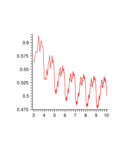
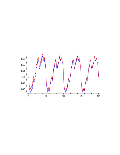
Figure 4. On the left the empirical (red) periodic function of Ex. 8 (mean discrepancy of the van der Corput sequence), and on the right the comparison between it and the theoretical (blue) periodic function computed by the cascade algorithm.

The coefficients of the asymptotic expansion of the running sum ${\mathbf{\Sigma}}_{N}$ inherit the properties of the coefficients of the asymptotic expansion of $\mathbf{S}_{K}(x)$. To see this we need to be more precise about the way we obtain the asymptotic expansion. Anew we use the same formalism as in Section 4.1.

Corollary 3.

Under Hypotheses 1 and 1 the asymptotic expansion of the running sum ${\mathbf{\Sigma}}_{N}$ associated with $V^{(\nu-1)}$ has coefficients which are Hölder with exponent $\log_{B}(\rho/\lambda)$ for $\lambda>\lambda_{*}$ and $\lambda$ may be replaced by $\lambda_{*}$ if $\lambda_{*}$ is attained.

Proof.

The only point which is to be verified is the continuity at integers, because up to this property the Hölderian character is evident (the coefficients are expressed as combinations of solutions of dilation equations and functions which are smooth except perhaps to integers). As we have seen the expansion of ${\mathbf{\Sigma}}_{N}$ comes from both terms in the right member of Formula (15). The first is $(\operatorname{I}_{d}-A_{0})\sum_{0\leq k\leq K}Q^{k}V^{(\nu-1)}$ and we do not want to expand it here, because the asymptotic expansion varies with the relative position of $\rho$, $\lambda_{*}$, and $1$. Moreover this is not necessary since it depends on $t$ only through $K$. The expansion of the second term is given by Formula (19). We note that this expression is merely the last column of the matrix $\mathbb{F}(B^{t-1})J_{\rho\omega}^{K+1}$ with the notations used in the proof of Lemma 4. Hence we are considering the matrix

$$\mathbb{A}(t)=(\operatorname{I}_{d}-A_{0})\sum_{0\leq k\leq K}Q^{k}V+\mathbb{F}(B^{t-1})J_{\rho\omega}^{K+1},$$

where $V$ is the matrix whose columns are the column vectors $V^{(0)}$ , $V^{(1)}$, $\ldots$, $V^{(\nu-1)}$ as in the proof of Lemma 4. The last column of the matrix $\mathbb{A}(t)$ is the regular part of the expansion of ${\mathbf{\Sigma}}_{N}$ (that is without the error term), and we want to verify that $t\mapsto\mathbb{A}(t)$ is a continuous function at integers. Let $K_{0}$ be an integer. When $t$ tends towards $K_{0}$ from above, we have $K=\lfloor t\rfloor=K_{0}$ and

$$\lim_{t\overset{>}{\rightarrow}K_{0}}\mathbb{A}(t)=(\operatorname{I}_{d}-A_{0})\sum_{0\leq k\leq K_{0}}Q^{k}V+\mathbb{F}(1/B)J_{\rho\omega}^{K_{0}+1},$$

but according to the dilation equation (12), $\mathbb{F}(1/B)=A_{0}VJ_{\rho\omega}^{-1}$ and we find

$$\lim_{t\overset{>}{\rightarrow}K_{0}}\mathbb{A}(t)=(\operatorname{I}_{d}-A_{0})\sum_{0\leq k\leq K_{0}}Q^{k}V+A_{0}VJ_{\rho\omega}^{K_{0}}.$$

On the other side when $t$ tends towards $K_{0}$ from below, we have $K=\lfloor t\rfloor=K_{0}-1$ and

$$\lim_{t\overset{<}{\rightarrow}K_{0}}\mathbb{A}(t)=(\operatorname{I}_{d}-A_{0})\sum_{0\leq k\leq K_{0}-1}Q^{k}V+\mathbb{F}(1)J_{\rho\omega}^{K_{0}}=(\operatorname{I}_{d}-A_{0})\sum_{0\leq k\leq K_{0}-1}Q^{k}V+VJ_{\rho\omega}^{K_{0}}.$$

The difference is

$$\lim_{t\overset{>}{\rightarrow}K_{0}}\mathbb{A}(t)-\lim_{t\overset{<}{\rightarrow}K_{0}}\mathbb{A}(t)=(\operatorname{I}_{d}-A_{0})Q^{K_{0}}V+(A_{0}-\operatorname{I}_{d})VJ_{\rho\omega}^{K_{0}}$$

but Hypothesis 1 writes $QV=VJ_{\rho\omega}$ and we conclude that the difference is the null matrix. ∎

Theorem C deserves some comments. Functions which roughly write $\Phi(t)=\omega^{K}\rho^{1-t}F(B^{t-1})$ have not the self-similar character of the solution  $F(x)$ of a dilation equation, because we have cut the piece of the function between $0$ and $1/B$. Moreover it is possible to use a more ordinary scale by expanding $\binom{\lfloor\log_{B}N\rfloor}{\ell}=\binom{-t+\log_{B}N}{\ell}$ as a polynomial in $\log_{B}N$ with coefficients in $t=\{\log_{B}N\}$. But doing this we hide completely the structure of the asymptotic expansion and the dilation equations which are behind it. This is certainly the reason why these equations have not been perceived before, even if the word “fractal” is frequently employed.

Example 9 [Coquet sequence].

The Coquet sequence (Coquet, 1983) is defined as $u(n)=(-1)^{s_{2}(3n)}$. (We recall that $s_{2}(n)$ is the sum of the bits in the binary expansion of $n$.)

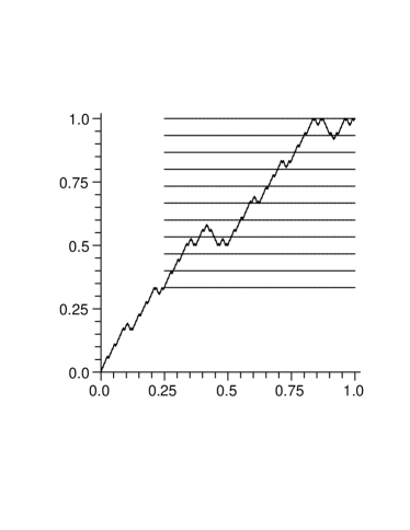
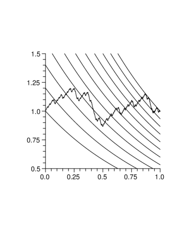
Figure 5. The change from the function $F(x)$ (left) to the periodic function $\Phi(t)$ (right) illustrated for the Coquet sequence.

It is $4$-rational and it admits (with $(u(n),u(4n+2),u(4n+3))$ as a generating family) the linear representation

$$A_{0}=\left(\begin{array}[]{ccc}1&1&1\\ 0&0&0\\ 0&0&0\end{array}\right),\qquad A_{1}=\left(\begin{array}[]{ccc}1&0&0\\ 0&1&-1\\ 0&0&0\end{array}\right),\qquad C=\left(\begin{array}[]{c}1\\ 0\\ 0\end{array}\right)\\ L=\left(\begin{array}[]{ccc}1&1&1\end{array}\right),\qquad A_{2}=\left(\begin{array}[]{ccc}0&0&0\\ 1&1&0\\ 0&0&1\end{array}\right),\qquad A_{3}=\left(\begin{array}[]{ccc}0&0&0\\ 0&0&0\\ 1&-1&1\end{array}\right).$$

The matrix

$$Q=A_{0}+A_{1}+A_{2}+A_{3}=\left(\begin{array}[]{ccc}2&1&1\\ 1&2&-1\\ 1&-1&2\end{array}\right)$$

has as eigenvalue  $3$, which is double, and $0$, which is simple. The joint spectral radius of the family $(A_{r})_{0\leq r<4}$ is $\lambda_{*}=1$, because with the maximum sum column norm we find $\lambda_{1}^{(1)}=1$ and  $1$ is an eigenvalue of each matrix $A_{r}$, $0\leq r<4$. The column vector $C$ decomposes as $C=V_{3}+V_{0}$, with

$$V_{3}=\left(\begin{array}[]{c}2/3\\ 1/3\\ 1/3\end{array}\right),\qquad V_{0}=\left(\begin{array}[]{c}1/3\\ -1/3\\ -1/3\end{array}\right)$$

and $V_{\rho}$ is an eigenvector for $\rho=3$, $0$.

Theorem C applies and we obtain (Coquet, 1983; Flajolet et al., 1994)

$$\sum_{n\leq N}(-1)^{s_{2}(3n)}\mathop{=}_{N\to+\infty}N^{\log_{4}3}\,3^{1-\{t\}}F(4^{\{t\}-1})+O(1),$$

with $t=\log_{4}N$. The function $F$ is the sum $F=F_{1}+F_{2}+F_{3}$, where $\mathbf{F}=(F_{1},F_{2},F_{3})$ is the unique solution of the dilation equation, written with Convention 2.4,

$$\left\{\begin{array}[]{l}F_{1}(x)=\displaystyle\frac{1}{3}F_{1}(4x)+\frac{1}{3}F_{2}(4x)+\frac{1}{3}F_{3}(4x)+\frac{1}{3}F_{1}(4x-1),\\[5.16666pt] F_{2}(x)=\displaystyle\frac{1}{3}F_{2}(4x-1)-\frac{1}{3}F_{3}(4x-1)+\frac{1}{3}F_{1}(4x-2)+\frac{1}{3}F_{2}(4x-2),\\[5.16666pt] F_{3}(x)=\displaystyle\frac{1}{3}F_{3}(4x-2)+\frac{1}{3}F_{1}(4x-3)-\frac{1}{3}F_{2}(4x-3)+\frac{1}{3}F_{3}(4x-3),\end{array}\right.$$

with the conditions $F_{1}(0)=F_{2}(0)=F_{3}(0)=0$, $F_{1}(1)=2/3$, $F_{2}(1)=F_{3}(1)=1/3$. The function $F(x)$ and the periodic function $\Phi(t)=3^{1-\{t\}}F(4^{\{t\}-1})$ are illustrated in Fig. 5 respectively on the left and on the right. The positive character of $\Phi$ proves a subtle phenomenon (Newman, 1969): the number of ones in the binary expansion of the integers which are multiple of $3$ is more often even than odd. Both functions are Hölder with exponent $\log_{4}3\simeq 0.795$. In the translation from $F$ to $\Phi$, the first quarter of $F$ is lost and $\Phi$ has not the auto-similar character of $F$.

As we have seen if the previous sections, it may be interesting to change the radix. Going from radix $B$ to radix $B^{T}$, we change the matrix $Q$ into its power $Q^{T}$. Frequently the eigenvalues of $Q$ have arguments which are commensurable with $\pi$ and a suitable choice of $T$ gives a matrix $Q$ whose all eigenvalues are real nonnegative. This trick is often used implicitly. For example the Coquet sequence is viewed as a $4$-rational sequence (as we have made in the previous example) in (Coquet, 1983; Dumont and Thomas, 1989; Allouche and Shallit, 2003) (but this is not the case in (Flajolet et al., 1994)). However it may be of interest to use two radices at a time. Even if both dilation equations define as well the function under consideration, it may be practically simpler to study the solution for one radix in terms of solutions for the other radix. The next example illustrates this point.

Example 10 [Rudin-Shapiro sequence continued].

As an application of Theorem C, we obtain the asymptotic expansion for the Rudin-Shapiro sequence defined in Ex. 1 (Brillhart et al., 1983)

$$\sum_{n\leq N}u_{n}\mathop{=}_{N\to+\infty}\sqrt{N}\Phi(\log_{4}N)+O(1)$$

where $\Phi$ is the $1$-periodic function defined by $\Phi(t)=2^{1-\{t\}}F(4^{\{t\}-1})$ and $F$ is defined through a dilation equation for radix $4$. Functions $F$ and $\Phi$ are illustrated in Fig. 6. Let us denote $\pi_{k}$ the part of the graph of $F$ which corresponds to the interval $[k/8,(k+1)/8]$ for $0\leq k<8$. It is evident that the parts of odd index on one side and the part of even index on the other side reproduce the same pattern (with a piece upside down) and we want to prove these facts.

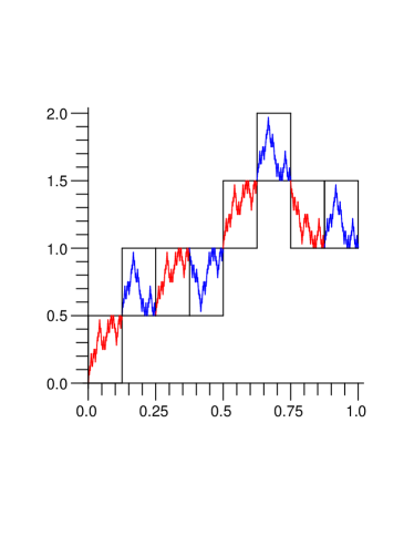
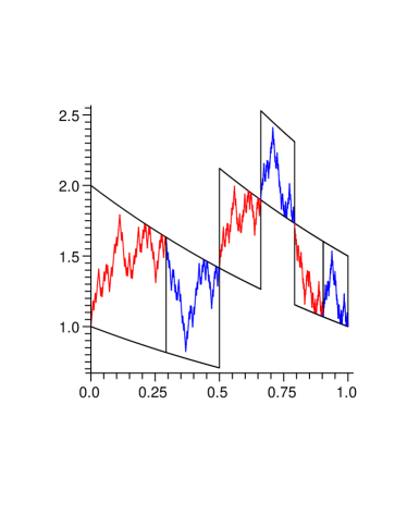
Figure 6. The solution of the dilation equation (left-hand side) and the periodic function (right-hand side) associated to the Rudin-Shapiro sequence show some symmetries.

Besides of radix $4$, we will use radix $2$. The matrix $Q$ for radix $2$ (see Ex. 1) has two eigenvalues $\pm\sqrt{2}$ and associated eigenvectors $V_{\pm}=(2\pm\sqrt{2},\pm\sqrt{2})/4$. The vector $C$ of the representation writes $C=V_{+}+V_{-}$ and we have to consider two vector-valued functions $\mathbf{F}_{\pm}$. Their components are $F_{\pm,1}$ and $F_{\pm,2}$. The function under study is $F=F_{+,1}+F_{+,2}+F_{-,1}+F_{-,2}$.

To abbreviate the computations and with the hope to make them clearer, we introduce the following formalism. The group of affine transforms of the real line acts on the vector space of functions from the real line into itself. More precisely the group acts on the right by substitution: for an affine transform $a$ and a function $f$, the image $f.a$ is simply the composed map $f\circ a$. As affine transforms it is natural in the actual context to consider $d_{0}:x\mapsto 2x$ and $d_{1}:x\mapsto 2x-1$. We will use $t_{1/2}:x\mapsto x+1/2$ too. With these notations the dilation equation for $\mathbf{F}_{\pm}$ writes (We use Convention 2.4 to write the dilation equations, that is we consider that functions are adequately extended to the whole real line.)

(20) $$F_{\pm,1}=\pm\frac{1}{\sqrt{2}}F_{\pm,1}.d_{0}\pm\frac{1}{\sqrt{2}}F_{\pm,2}.d_{0},\qquad F_{\pm,2}=\pm\frac{1}{\sqrt{2}}F_{+,1}.d_{1}\mp\frac{1}{\sqrt{2}}F_{\pm,2}.d_{1},$$

with the conditions $\mathbf{F}_{\pm}(0)=0$ and $\mathbf{F}_{\pm}(1)=V_{\pm}$ We will collect some simple facts in order to achieve our goal. It results from the dilation equations that $F_{\pm,2}$ is $0$ on the left of $1/2$, while $F_{\pm,1}$ is constant on the right of $1/2$. The action of $t_{1/2}$ on both members of the second equation above with the equality $d_{1}\circ t_{1/2}=d_{0}$ provides

$$F_{+,2}.t_{1/2}=\frac{1}{\sqrt{2}}F_{+,1}.d_{0}-\frac{1}{\sqrt{2}}F_{+,2}.d_{0}.$$

A subtraction and an addition give respectively

(21) $$F_{+,1}-F_{+,2}.t_{1/2}=\sqrt{2}F_{+,2}.d_{0},\qquad F_{+,1}+F_{+,2}.t_{1/2}=\sqrt{2}F_{+,1}.d_{0}.$$

From these preliminaries follow the following formulæ

(22) $$\begin{array}[]{llll}F\left(x+\frac{1}{2}\right)-F(x)=1,&\text{for $0\leq x\leq\frac{1}{4}$},&\qquad F\left(x+\frac{1}{2}\right)+F(x)=2,&\text{for $\frac{1}{4}\leq x\leq\frac{1}{2}$},\\[6.88889pt] F\left(x+\frac{1}{4}\right)-F(x)=\frac{1}{2},&\text{for $\displaystyle 0\leq x\leq\frac{1}{8}$},&\qquad F\left(x+\frac{1}{4}\right)+F(x)=\frac{3}{2},&\text{for $\displaystyle\frac{1}{8}\leq x\leq\frac{1}{4}$}.\end{array}$$

We prove only the third one; the other proof are of the same type. For $0\leq x\leq 1/8$, the number $x+1/4$ lies in $[1/4,3/8]$ and both numbers are in $[0,1/2]$. The dilation equations (20) give

$$F_{\pm,1}(x)=\pm\frac{1}{\sqrt{2}}F_{\pm,1}(2x)\pm\frac{1}{\sqrt{2}}F_{\pm,2}(2x),\qquad F_{\pm,2}(x)=0,$$

and

$$F_{\pm,1}\left(x+\frac{1}{4}\right)=\pm\frac{1}{\sqrt{2}}F_{\pm,1}\left((2x+\frac{1}{2}\right)\pm\frac{1}{\sqrt{2}}F_{\pm,2}\left(2x+\frac{1}{2}\right),\quad\displaystyle F_{\pm,2}\left(x+\frac{1}{4}\right)=0.$$

Since $F$ is $F_{+,1}+F_{+,2}+F_{-,1}+F_{-,2}$, we obtain

$$F\left(x+\frac{1}{4}\right)-F(x)=\frac{1}{\sqrt{2}}\left[F_{+,1}\left(2x+\frac{1}{2}\right)+F_{+,2}\left(2x+\frac{1}{2}\right)\right.\\ \left.-F_{-,1}\left(2x+\frac{1}{2}\right)-F_{-,2}\left(2x+\frac{1}{2}\right)-F_{+,1}(2x)-F_{+,2}(2x)+F_{-,1}(2x)+F_{-,2}(2x)\right].$$

However $2x$ is in $[0,1/4]$ and $2x+1/2$ is in $[1/2,3/4]$. The functions $F_{\pm,1}$ are constant on the right of $1/2$, while the functions $F_{\pm,2}$ are constant on the left of $1/2$. Making explicit theses constant values, we obtain

$$F\left(x+\frac{1}{4}\right)-F(x)=\frac{1}{\sqrt{2}}\left[\frac{1}{2}\sqrt{2}-F_{+,1}(2x)+F_{-,1}(2x)+F_{+,2}\left(2x+\frac{1}{2}\right)-F_{-,2}\left(2x+\frac{1}{2}\right)\right].$$

Besides Formula (21) gives

$$F_{\pm,1}(2x)=F_{\pm,2}\left(2x+\frac{1}{2}\right)$$

because $x$ is in $[0,1/8]$. The expected formula is proved.

The previous computations ask some questions. We have established formulæ  which write

$$\sum_{f,a}\lambda_{f,a}f.a=c,$$

where $f$ runs through the four functions $F_{+,1}$, $F_{+,2}$, $F_{-,1}$, $F_{-,2}$; $a$ runs through the set of affine transforms of the real line; the family $(\lambda_{f,a})$ has a finite support; $c$ is some constant. Is it possible to design a method in order to find such relationships? For example, how to obtain mechanically the formula

$$\frac{4}{2+\sqrt{2}}F_{\pm,1}(x)-\frac{4}{\sqrt{2}}F_{\mp,2}(1-x)=1?$$

Does exists a regular process which gives formulæ  of the type

$$\sum_{a}\lambda_{a}F.a=C?$$

Evidently we want a minimal generating set for such formulæ.

From the four formulæ (22) above we deduce that all pieces of the graph of $F$ are obtained from $\pi_{0}$ and $\pi_{1}$ by some translations or glide reflections. The symmetries of $F$ are translated to $\Phi$, but they lose their graphical evidence. The pieces $\pi_{0}$ and $\pi_{1}$ disappear and the pieces $\pi_{k}$, $2\leq k<8$ become the pieces $\pi_{k}^{\prime}$ associated to the interval $[\log_{4}(k/2),\log_{4}((k+1)/2)]$. The links between the pieces become more intricate. For example the pieces $\pi_{2}^{\prime}$ and $\pi_{3}^{\prime}$ on one side and $\pi_{6}^{\prime}$ and $\pi_{7}^{\prime}$ on the other side are linked by the formula $2^{s}\Phi(s)+2^{t}\Phi(t)=4$ under the condition that both numbers $s\in[0,1/2]$ and $t\in[\log_{4}3,1]$ are related by $4^{t}-4^{s}=2$.

Example 11 [Rescaling].

In the study of radix-rational sequences, it is an attractive idea at first sight to multiply all the matrices $A_{0}$, $\ldots$, $A_{B-1}$ of a linear representation by a scalar in order to control the order of growth of the sequence. But after a while the idea seems to be silly, because it introduces a weighting according to the length of the radix $B$ expansions of the integers. The previous theorem shows clearly the effect of such a rescaling. It appears that the modification does not change at all the functions $F(x)$ defined by a dilation equation, and changes very simply the periodic functions $\Phi(t)$.

Let us consider the sequence $u(n)=n$. It admits the representation

$$L=\left(\begin{array}[]{cc}0&1\end{array}\right),\quad A_{0}=\left(\begin{array}[]{cc}{B}&0\\ 0&1\end{array}\right),\quad A_{r}=\left(\begin{array}[]{cc}{B}&0\\ r&1\end{array}\right)\;\text{for $r>0$,}\quad C=\left(\begin{array}[]{c}1\\ 0\end{array}\right).$$

for radix $B$. There is a dominant eigenvalue $\rho={B}^{2}$, with associated functions $F(x)=x^{2}$ and $\Phi(t)=1/2$. We obtain the obvious asymptotic expansion

$$\sum_{n\leq N}n\mathop{=}_{N\to+\infty}\frac{1}{2}N^{2}+O(N).$$

Now consider the sequence $u(n)=n/{B}^{\lambda_{B}(n)}$, where $\lambda_{B}(n)$ is the length of the radix ${B}$ expansion of $n$. With ${B}=2$ it begins with $0$, $0.1$, $0.10$, $0.11$, $0.100$, $0.101$, $0.110$, $0.111$, $0.1000$, $\ldots$ It admits the representation

$$L=\left(\begin{array}[]{cc}0&1\end{array}\right),\quad A_{0}=\left(\begin{array}[]{cc}1&0\\ 0&1/{B}\end{array}\right),\quad A_{r}=\left(\begin{array}[]{cc}1&0\\ r/{B}&1/{B}\end{array}\right)\;\text{for $r>0$,}\quad C=\left(\begin{array}[]{c}1\\ 0\end{array}\right)$$

and again we have $F(x)=x^{2}$, but $\rho={B}$. We obtain the less obvious asymptotic expansion

$$\sum_{n\leq N}\frac{n}{B^{\lambda_{B}(n)}}\mathop{=}_{N\to+\infty}\frac{1}{2}N\Phi(\log_{B}N)+O(1)$$

with

$$\Phi(t)=\frac{{B}^{-t}+{B}^{t-1}}{2}=\frac{1}{{B}^{1/2}}\cosh\left((t-\frac{1}{2})\ln{B}\right),\qquad\text{for $0\leq t<1$.}$$

The convergence towards this function is illustrated in Fig. 7 where a (piece of) catenary appears in an evident way.

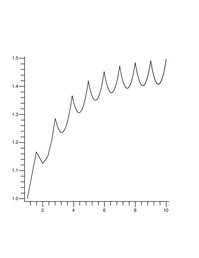
Figure 7. The empirical periodic function for sequence $u(n)=n/2^{\lambda_{2}(n)}$ (where $\lambda_{2}(n)=1+\lfloor\log_{2}n\rfloor$ is the length of the binary expansion of $n$) as a function of $\log_{2}n$. A catenary appears.

5.2. Substitutions and automata

In the very beginning of the introduction we have written that nobody has asserted a general theorem about the asymptotic expansion of radix-rational sequences. This is not quite the truth because Allouche and Shallit (2003, Sec. 3.5) provide a theorem. But their statement suffers from a severe restriction because they assume for example the hypothesis $A_{w}=O(K)$ for $\lvert w\rvert=K$, that is $\lambda_{*}\leq 1$, and some other technical hypotheses. It is noteworthy that the result they give has no error term and for this it appears as a direct generalization of (Delange, 1975).

Other works which deserve attention are related to the name of Dumont (Dumont and Thomas, 1989; Dumont, 1990; Dumont et al., 1999). There is a link between these works and the present one, but it needs some explanations to be emphasized. We consider a finite alphabet $\mathcal{X}$. A substitution $\sigma$ on $\mathcal{X}$ is a map which associates to each letter a non empty word. It extends as a morphism of $\mathcal{X}^{*}$ by concatenation. If $a$ is a letter which turns out to be a strict prefix of the word $\sigma(a)$, the sequence $(\sigma^{k}(a))$, obtained by iteration of $\sigma$ from $a$, converges to an infinite word $\omega=(\omega_{n})_{n\geq 0}$, which is named a fixed point of $\sigma$ (Fogg, 2002).

We may associate to the substitution $\sigma$ and to the letter $a$ an automaton $\mathcal{A}_{\sigma}$. The state of the automaton are the letters of the alphabet. There is a unique initial state which is the letter $a$. All states are final states. The transitions are labeled by nonnegative integers and obtained in the following way. For a letter $x$, the non empty word $\sigma(x)$ has length $\ell\geq 1$ and writes $\sigma(x)=\sigma_{0}(x)\sigma_{1}(x)\ldots\sigma_{\ell-1}(x)$. There is a transition from state $x$ to state $\sigma_{r}(x)$ labeled by $r$. Conversely the automaton determines the substitution and the fixed point of the substitution which begins by $a$. If $B$ is the maximal length of the words $\sigma(x)$ for $x$ a letter, all labels are bounded above by $B-1$. To the automaton is associated the language $\mathcal{L}$ it recognizes, that is the set of words over the alphabet $\left\{0,1,\ldots,B-1\right\}$ which translate a sequence of transitions from the initial state to a final state. This language is regular because it is recognized by the automaton. The simplest case is the case where the substitution is of constant length, which means that all words $\sigma(x)$, $x\in\mathcal{X}$, have the same length $B\geq 2$. In such a case the language $\mathcal{L}$ is merely the free monoid $\left\{0,1,\ldots,B-1\right\}^{*}$.

The automaton may be enriched by an output function $f$ which associates to each state, that is letter, a value. The output function extends to words and the image of the fixed point $\omega$ is an infinite sequence of values. Dumont and Thomas (1989) study the asymptotic behaviour of the running sum

$$S^{f}(N)=\sum_{0\leq n<N}f(\omega_{n})$$

where $f$ is real-valued, under some hypotheses which we will describe later.

To merge the framework of (Dumont and Thomas, 1989) and ours it suffices to consider a linear version of the automaton. For a given commutative field $\mathbb{K}$, we consider the space $\mathbb{K}^{\mathcal{X}}$, whose canonical base is $(e_{x})_{x\in\mathcal{X}}$. To each integer $r$ between $0$ and $B-1$ we associate a $d\times d$ matrix $A_{r}$, where $d$ is the size of the alphabet, defined by $A_{r}e_{x}=e_{y}$ if there is a transition labeled $r$ from state $x$ to state $y$ in the automaton, and $A_{r}e_{x}=0$ otherwise. The matrix $Q=A_{0}+\dotsb+A_{B-1}$ is the incidence matrix of the substitution; its entries $Q_{x,y}$ is the number of occurrences of the letter $y$ in the word $\sigma(x)$. We insert in the description the column vector $C=e_{a}$ and the row vector $L=(f(x))_{x\in\mathcal{A}}$ and we have a linear representation. For a word $w=w_{0}\dotsb w_{K-1}$ taken from the language $\mathcal{L}$ of the automaton, it is equivalent to follow from the initial state $a$ the transitions labeled $w_{0}$, $\ldots$, $w_{K-1}$ and to compute the value $f(z)$ of the state $z$ where ends the path, or to compute the matrix product $LA_{w_{K-1}}\dotsb A_{w_{0}}C$. We are not far to the definition of a radix-rational sequence, but the idea of a numeration system is yet lacking.

The lengths of the iterates $\sigma^{n}(a)$ are the elements of an increasing sequence $\mathcal{B}=(B_{n})_{n\geq 0}$ which begins with $B_{0}=1$. This sequence defines a numeration system: a nonnegative integer $n$ admits an expansion $(a_{K-1}\ldots a_{0})_{\mathcal{B}}$ in the system $\mathcal{B}$ if it writes $n=a_{0}B_{0}+a_{1}B_{1}+\dotsb+a_{K-1}B_{K-1}$. There is always at least one expansion named the normal $\mathcal{B}$-representation, which is obtained by a greedy algorithm. The language $\mathcal{S}$ associated to the system of numeration is the set of all normal $\mathcal{B}$-representations of nonnegative integers. (The representation of $0$ is the empty word.) Generally speaking, the language $\mathcal{L}$ is not regular and is distinct form the language $\mathcal{S}$, but in the simple case where the substitution is of constant length $B$, both languages $\mathcal{L}$ and $\mathcal{S}$ are equal. As a consequence the sequence $(f(\omega_{n}))$ is $B$-rational. It is even $B$-automatic: for an nonnegative integer $n$ we write its radix $B$ expansion and we use this word to follow a path which begins with $a$ in the automaton; the end of the path is $\omega_{n}$ and the value associated to $n$ is $f(\omega_{n})$. It is proved that a $B$-automatic sequence is a $B$-rational sequence which takes a finite number of values.

Nevertheless the previous system of numeration is not suitable in case of a substitution which is not of constant length. The prefix-suffix automaton $\mathcal{A}^{\prime}_{\sigma}$ (Mossé, 1996; Canterini and Siegel, 2001) is the right automaton. Its states are the letters of $\mathcal{X}$. There is a transition labeled $(p,x,s)\in\mathcal{X}^{*}\times\mathcal{X}\times\mathcal{X}^{*}$ from $x$ to $y$ if $\sigma(y)=pxs$ (hence the name of the automaton). All states are initial and $a$ is the only final states. Clearly $\mathcal{A}^{\prime}_{\sigma}$ is a sophisticated version of $\mathcal{A}$ (the transitions are reversed but this is of no importance), which is equivalent in case of a substitution of constant length. Dumont and Thomas (1989) use a version of this automaton which takes into account only the prefixes. The language $\mathcal{L}^{\prime}$ recognized by $\mathcal{A}^{\prime}_{\sigma}$ may be defined by a set of prohibited patterns: a pair of labels $((p,x,s),(p^{\prime},y,s^{\prime}))$ such that $\sigma(y)\neq psx$ does not occur in a word of $\mathcal{L}^{\prime}$. For every subword $\omega^{N}=(\omega_{n})_{0\leq n<N}$ there exists a unique path $((p_{k},x_{k},s_{k}))_{0\leq k<K}$ of length $K$, determined by $B_{K}\leq N<B_{K+1}$, which ends at $a$. In other terms there exists a unique word $((p_{k},x_{k},s_{k}))_{0\leq k<K}$ from $\mathcal{L}^{\prime}$ of length $K$ such that $x_{K-1}=a$. It defines a cutting of $\omega^{N}=(\omega_{n})_{0\leq n<N}$ which writes $\omega^{N}=\sigma^{K-1}(p_{K-1})\sigma^{K-2}(p_{K-2})\ldots\sigma^{0}(p_{0})$. Moreover the prefixes $p_{k}$ lie in the finite set of strict prefixes of the words $\sigma(x)$ with $x$ a letter. Such a result demands hypotheses (Mossé, 1992): the substitution is primitive, which means that there exists a $k$ such that for every pair of letters $x$ and $y$ the letter $x$ occurs in $\sigma^{k}(y)$; the fixed point $\omega$ is not a periodic sequence. Taking into account the lengths of the words, we obtain $N=|\sigma^{K-1}(p_{K-1})|+|\sigma^{K-2}(p_{K-2})|+\dotsb+|\sigma^{0}(p_{0})|$. This is the expansion of the integer $N$ according to the numeration system associated with the substitution $\sigma$ and $a$. (Note that there does not exist a general definition of what is a numeration system.) The proof of the existence of the expansion is anew a greedy algorithm (Dumont and Thomas, 1989, Lemma 1.3): $p_{K-1}$ is the longest prefix of $\omega$ such that $\sigma^{K-1}(p_{K-1})$ is a prefix of $\omega^{N}$.

The asymptotic study of the sequence $(S^{f}(N))_{N\geq 0}$ is based on the following remarks. The function $f$ is defined on the letters of the alphabet $\mathcal{X}$ and extends additively to the word of $\mathcal{X}^{*}$. Particularly we have $S^{f}(N)=f(\omega^{N})$. Let $L$ the row vector whose entries are the values of $f$ on the letters of the alphabet; let $C_{w}$ the column whose entries are the number of occurrences of each letter in the word $w$. A consequence of these definition is the formula $f(w)=LC_{w}$. Let $Q$ be the incidence matrix of the substitution $\sigma$. We see immediately the recursion $C_{\sigma(w)}=QC_{w}$. As a consequence we have two analogous formulæ

$$S^{f}(N)=f(\omega^{N})=L\sum_{k=0}^{K-1}Q^{k}C_{p_{k}},\qquad N=U\sum_{k=0}^{K-1}Q^{k}C_{p_{k}},$$

where $U$ is the row vector whose all entries are equal to $1$. Both formulæ  render plausible the following result (Dumont and Thomas, 1989, Th. 2.6),

$$S^{f}(N)\mathop{=}_{N\to+\infty}L\Lambda\,N+\log_{\theta}^{\alpha}NN^{\beta}G(N)+o(\log_{\theta}^{\alpha}NN^{\beta}).$$

It is proved under the following hypotheses and through the following assertions. Because $Q$ is a primitive nonnegative matrix, its spectral radius $\theta$ is a dominant eigenvalue. The column vector $\Lambda$ is its positive eigenvector, normalized by $U\Lambda=1$. The existence of a sub-dominant eigenvalue $\theta^{\prime}$ is assumed. It dominates all others eigenvalues apart $\theta$, that is $\theta>\theta^{\prime}>|\theta^{\prime\prime}|$ for all eigenvalues $\theta^{\prime\prime}$ except $\theta$ and $\theta^{\prime}$. Moreover it is assumed $\theta^{\prime}>1$. The integer $\alpha$ is defined such that $\alpha+1$ is the multiplicity of $\theta^{\prime}$ as root of the minimal polynomial of $Q$ and the real number $\beta$ is defined by $\beta=\log_{\theta}\theta^{\prime}$. The function $G$ is defined as the limit

$$\forall x>0,\quad G(x)=x^{-\beta}\lim_{k\to+\infty}\frac{S^{f}(\lfloor\theta^{k}x\rfloor)-L\Lambda\lfloor\theta^{k}x\rfloor}{k^{\alpha}\theta^{\prime}{}^{k}}.$$

It satisfies $G(\theta x)=G(x)$ for $x$ positive and is Hölder of exponent $\beta$.

To summarize Dumont and Thomas (1989) study the mean asymptotic behaviour of real-valued sequences defined by substitutions and for substitutions with constant length this reduces to automatic sequences. We study complex-valued sequences associated to complex rational formal power series and for series which takes only a finite number of values this reduces to automatic sequences.

5.3. Linear representation insensitive to the leftmost zeroes

In the use of Formula (13), we may introduce a simplifying hypothesis which turns out to be non restrictive. To a rational formal series we associate a radix-rational series through a numeration system. But the knowledge of a radix-rational sequence does not determine a unique rational formal series, because the expansions of the integers does not use the words which begin with a zero. A first idea which comes in mind to complete the definition of the formal series is to decide that words which begin with zero give a null value. But there is another way to extend a radix-rational sequence into a formal series and it is more natural after all. Let us say that a linear representation of a radix-rational series is insensitive to the leftmost zeroes if it satisfies $LA_{0}=L$. For such a representation the formal power series is completely determined by the radix-rational series, because the adding of some zeroes on the left of the expansion of an integer does not change the value associated to this word.

Lemma 10.

Every radix-rational sequence has a (reduced) linear insensitive to the leftmost zeroes representation, that is a representation such that $LA_{0}=L$.

This point is described in (Dumas, 1993, sec. 4.2) (where an insensitive to the leftmost zeroes representation is termed standard), but we give a proof because it explains how most of the linear representations in this paper are obtained.

Proof.

For the sake of simplicity, let us assume that the radix is $B=2$. The hypothesis is that all subsequences $(u_{2^{k}n+r})$, $k\geq 0$, $0\leq r<2^{k}$, of the radix-rational sequence $(u_{n})$ generate a finite dimensional vector space $U$. Let $d$ be the dimension of that vector space. (For the null sequence, we have $d=0$. We exclude this case.) We consider the subsequences $(u_{n})$, $(u_{2n})$, $(u_{2n+1})$, $(u_{4n})$, $(u_{4n+1})$, $(u_{4n+2})$, $\ldots$ in that order and the dimension $d_{j}$ of the vector space generated by the $j$ first subsequences (with $d_{-1}=0$). We select the subsequences $v^{1}$, $v^{2}$, $\ldots$, $v^{d}$ such that the dimension increases by $1$ when they encountered in the previous list. The family $(v^{\ell})_{1\leq\ell\leq d}$ is a basis of $U$. The sequence $(u_{n})$ expresses as a linear combination of $v^{1}$, $v^{2}$, $\ldots$, $v^{d}$ (the sequence $(u_{n})$ is nothing but $v^{1}$), and this gives the column vector $C$ of the linear representation we are building. Next we consider the action of $0$ and $1$ over the sequences $v^{\ell}$ defined by $(0.v^{\ell})_{n}=v^{\ell}_{2n}$ and $(1.v^{\ell})_{n}=v^{\ell}_{2n+1}$ and we express the images in the basis $(v^{\ell})_{1\leq\ell\leq d}$. This gives the square matrices $A_{0}$ and $A_{1}$ of the representation. At last the row vector $L$ is the vector of initial values $v^{\ell}_{0}$. In that way, we have a linear representation of the sequence $(u_{n})$. This may be readily verified by considering the sequence of row vectors $\Lambda_{n}=(v^{1}_{n},\,v^{2}_{n},\ \ldots\ v^{d}_{n})$ which satisfies $u_{n}=\Lambda_{n}C$, $\Lambda_{2n}=\Lambda_{n}A_{0}$, $\Lambda_{2n+1}=\Lambda_{n}A_{1}$, $L=\Lambda_{0}$. (Note that Allouche and Shallit (2003) use a column vector for $\Lambda_{n}$, hence the transposed matrices for $A_{0}$, $A_{1}$.) Moreover the equation $(0.v^{\ell})_{0}=v^{\ell}_{0}$, that is $\Lambda_{0}A_{0}=\Lambda_{0}$, renders evident the formula $LA_{0}=L$. The proof would be more enlightening by considering a binary tree and a prefix part of the monoid of words, but we will not insist on this point. ∎

We do not have used this hypothesis of insensitivity in the proofs because it is unsuitable for the vector-valued version we have elaborated, but most of the examples we have given have this property and this saves us to compute the first term of Formula (13).

5.4. Periodicity versus pseudo-periodicity

The occurrence of periodic functions in logarithmic scale is common in the asymptotic study of radix-rational sequences (Coquet, 1983; Delange, 1975; Dumont et al., 1999; Flajolet and Golin, 1994; Flajolet et al., 1994; Osbaldestin and Shiu, 1989). Nevertheless the rising of periodic functions, if true in practical examples, is wrong in full generality. The reason is the following: in common examples the eigenvalues of the matrix $Q$ have arguments which are commensurable with $\pi$. As we have already explained, a change of radix permits to consider that the useful eigenvalues are all positive numbers. As a consequence functions $\Phi$ are periodic, because they depend only on the fractional part of the variable $t$. But in the general case they write something like $\Phi(t)=\omega^{\lfloor t\rfloor}\rho^{1-\{t\}}F(B^{\{t\}-1})$ and if $\omega$ does not write $\omega=e^{i\vartheta}$ with $\vartheta/\pi$ a rational number, the function $\Phi$ is not periodic but only pseudo-periodic. Below we exemplify this phenomenon.

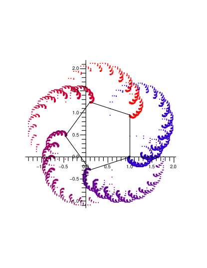
Figure 8. The empirical rosette of Ex. 12 with $\vartheta=2\pi/5$. For each frond of the rosette, the index $N$ goes from $2^{K}$ to $2^{K+1}-1$. Here $K$ goes from $11$ to $15$ and the color from red to blue. The vertices of the pentagon are the points ${\mathbf{\Gamma}}(K)$ with $K$ integer.

Example 12 [Rosettes].

Let us consider the linear representation for radix $B=2$ and dimension $2$,

$$A_{0}=\left(\begin{array}[]{cc}\cos{\vartheta}&0\\ 0&\cos{\vartheta}\end{array}\right),\qquad A_{1}=\left(\begin{array}[]{cc}0&-\sin{\vartheta}\\ \sin{\vartheta}&0\end{array}\right),$$

where $\vartheta$ is a real number restricted by the condition $\vartheta\not\equiv 0\bmod\pi/2$ to avoid degeneracy. We do not define the row vector $L$, because we are interested in the vector-valued sequence

$${\mathbf{\Sigma}}_{N}=\sum_{0\leq n\leq N}A_{w}C$$

($w$ is the binary expansion of the integer $n$). With regard to the column vector $C$, we note that both matrices $A_{0}$ and $A_{1}$ write $A_{0}=\cos\vartheta\,\operatorname{I}_{2}$, $A_{1}=\sin\vartheta\,R_{\pi/2}$ (notation of Ex. 5: $R_{\varphi}$ is the rotation matrix with angle $\varphi$). As a consequence they commute with all rotation matrices and if $C$ is changed into $R_{\varphi}C$, then ${\mathbf{\Sigma}}_{N}$ is changed into $R_{\varphi}{\mathbf{\Sigma}}_{N}$. Evidently we have a similar formula with dilations and so we may take as vector $C$ the first vector $E_{1}$ of the canonical basis.

The joint spectral radius is $\lambda_{*}=\max(|\cos{\vartheta}|,|\sin{\vartheta}|)$, because $\left\|A_{0}\right\|_{1}=|\cos{\vartheta}|$, $\left\|A_{1}\right\|_{1}=|\sin{\vartheta}|$ and $A_{0}^{2}$ and $A_{1}^{2}$ admit respectively the eigenvalues $\cos^{2}{\vartheta}$ and $-\sin^{2}{\vartheta}$. The matrix $Q=A_{0}+A_{1}$ is the rotation matrix $R_{\vartheta}$ and its eigenvalues are $\rho\omega_{\pm}$ with $\rho=1$ and $\omega_{\pm}=e^{\pm i\vartheta}$. We take as eigenvectors respectively for $\omega_{+}$ and $\omega_{-}$ the vectors $V_{+}=\left(\begin{array}[]{cc}1&-i\end{array}\right)^{\mathrm{tr}}$, $V_{-}=\left(\begin{array}[]{cc}1&i\end{array}\right)^{\mathrm{tr}}$. The vector $C$ expands as $C=(V_{+}+V_{-})/2$. We have $\lambda_{*}<\rho$ and Theorem C applies. The asymptotic expansion for the sum ${\mathbf{\Sigma}}_{+,N}$ associated with $V_{+}$ writes

$${\mathbf{\Sigma}}_{+,N}=(\operatorname{I}_{2}-A_{0})\sum_{k=0}^{K}Q^{k}V_{+}+e^{i(K+1)\vartheta}\mathbf{F}_{+}(2^{\{t\}-1})+O(\lambda_{*}^{K}),$$

where $\mathbf{F}_{\pm}$ is defined by the dilation equation

$$\left\{\begin{array}[]{l}F_{{\pm},1}(x)=\cos{\vartheta}e^{\mp i\vartheta}F_{{\pm},1}(2x),\\ F_{{\pm},2}(x)=\cos{\vartheta}e^{\mp i\vartheta}F_{{\pm},2}(2x),\end{array}\right.\quad\text{for $0\leq x<\frac{1}{2}$;}\\ \left\{\begin{array}[]{l}F_{{\pm},1}(x)=\cos{\vartheta}e^{\mp i\vartheta}-\sin{\vartheta}e^{\mp i\vartheta}F_{{\pm},2}(2x-1),\\ F_{{\pm},2}(x)=\mp i\cos{\vartheta}e^{\mp i\vartheta}+\sin{\vartheta}e^{\mp i\vartheta}F_{{\pm},1}(2x-1),\end{array}\right.\quad\text{for $\frac{1}{2}\leq x<1$,}$$

with the boundary conditions $\mathbf{F}_{\pm}(0)=0$, $\mathbf{F}_{\pm}(1)=V_{\pm}$. Both vector-valued functions $\mathbf{F}_{\pm}$ are conjugate. Emphasizing their real and imaginary parts $\mathbf{U}$ and $\pm\mathbf{V}$ and carrying on with the computation we obtain for the sum ${\mathbf{\Sigma}}_{N}$ associated with $C=E_{1}$ the asymptotic expansion

$${\mathbf{\Sigma}}_{N}\mathop{=}_{N\to+\infty}{\mathbf{\Gamma}}(t)+O(\lambda_{*}^{K}),$$

with ${\mathbf{\Gamma}}:t\mapsto\Omega+\mathbf{A}(t)+\mathbf{B}(t)$,

$$\Omega=\sin\frac{\vartheta}{2}\left(\begin{array}[]{c}\sin\vartheta/2\\ \cos\vartheta/2\end{array}\right),\qquad\mathbf{A}(t)=\sin\frac{\vartheta}{2}\left(\begin{array}[]{c}\cos((K+1/2)\vartheta-\pi/2)\\ \sin((K+1/2)\vartheta-\pi/2)\end{array}\right),$$

$$\mathbf{B}(t)=\cos((K+1)\vartheta)\,\mathbf{U}(2^{\{t\}-1})-\sin((K+1)\vartheta)\,\mathbf{V}(2^{\{t\}-1}).$$

Obviously an increasing of $t$ (and consequently of $K$) by $1$ rotates the vector $\mathbf{A}(t)$ by $\vartheta$. The change for $\mathbf{B}$ is less obvious. From the real point of view, the dilation equation for $\mathbf{F}_{+}$ rewrites

$${\mathbf{\Phi}}(x)=T_{0}{\mathbf{\Phi}}(2x)\qquad\text{for $0\leq x<\frac{1}{2}$},\qquad{\mathbf{\Phi}}(x)=T_{0}W+T_{1}{\mathbf{\Phi}}(2x-1)\qquad\text{for $\frac{1}{2}\leq x<1$,}$$

where ${\mathbf{\Phi}}$ is the $4$-dimensional vector-valued function ${\mathbf{\Phi}}=\left(\begin{array}[]{cc}\mathbf{U}&\mathbf{V}\end{array}\right)^{\mathrm{tr}}$. The matrices $T_{0}$ and $T_{1}$ have the following expressions

$$T_{0}=\left(\begin{array}[]{cccc}\cos^{2}{\vartheta}&0&\cos{\vartheta}\sin{\vartheta}&0\\ 0&\cos^{2}{\vartheta}&0&\cos{\vartheta}\sin{\vartheta}\\ -\cos{\vartheta}\sin{\vartheta}&0&\cos^{2}{\vartheta}&0\\ 0&-\cos{\vartheta}\sin{\vartheta}&0&\cos^{2}{\vartheta}\end{array}\right)=\cos{\vartheta}\,R_{-\vartheta}\otimes\operatorname{I}_{2},$$

$$T_{1}=\left(\begin{array}[]{cccc}0&-\cos{\vartheta}\sin{\vartheta}&0&-\sin^{2}{\vartheta}\\ \cos{\vartheta}\sin{\vartheta}&0&\sin^{2}{\vartheta}&0\\ 0&\sin^{2}{\vartheta}&0&-\cos{\vartheta}\sin{\vartheta}\\ -\sin^{2}{\vartheta}&0&\cos{\vartheta}\sin{\vartheta}&0\end{array}\right)=\sin{\vartheta}\,R_{-\vartheta}\otimes R_{\pi/2}.$$

The boundary conditions are ${\mathbf{\Phi}}(0)=0$ and ${\mathbf{\Phi}}(1)=W$ with $W=\left(\begin{array}[]{cccc}1&0&0&-1\end{array}\right)^{\mathrm{tr}}$. Let $P$ be the matrix

$$P=\left(\begin{array}[]{cccc}0&0&0&-1\\ 0&0&1&0\\ 0&1&0&0\\ -1&0&0&0\end{array}\right).$$

We verify $P^{-1}T_{0}P=T_{0}$, $P^{-1}T_{1}P=T_{1}$, $PW=W$. As a result $P{\mathbf{\Phi}}$ is a solution of the dilation equation. But the dilation equation has a unique solution and we conclude that ${\mathbf{\Phi}}$ satisfies $P{\mathbf{\Phi}}={\mathbf{\Phi}}$. This means $-\mathbf{V}=R_{\pi/2}\mathbf{U}$. This shows the formula $\mathbf{B}(t+1)=R_{\vartheta}\mathbf{B}(t)$. Eventually we see that ${\mathbf{\Gamma}}(t+1)$ is the image of ${\mathbf{\Gamma}}(t)$ by the rotation of angle $\vartheta$ about $\Omega$.

Let us assume that $\vartheta$ is commensurable with $\pi$, and let us write $\vartheta/\pi=p/q$ where $p/q$ is in lowest terms. We see immediately that the arc ${\mathbf{\Gamma}}$ is $2q$-periodic, and even $2^{1-\kappa}q$-periodic if $\kappa$ is the dyadic valuation of $p$. This phenomenon is illustrated by Fig. 8. Besides it is easy to verify ${\mathbf{\Gamma}}(t+2^{-\kappa}q)+{\mathbf{\Gamma}}(t)=2\Omega$.

To the contrary when the ratio $\vartheta/\pi$ is irrational, the rotation $R_{\vartheta}$ leaves invariant the image of the arc ${\mathbf{\Gamma}}$ but its order is infinite. The non-periodic character of the arc ${\mathbf{\Gamma}}$ is evident when we consider its value at integers,

$${\mathbf{\Gamma}}(K)=\Omega+\cos\frac{\vartheta}{2}\left(\begin{array}[]{c}\cos(K-1/2)\vartheta\\ \sin(K-1/2)\vartheta\end{array}\right).$$

Hence we see that the functions $\Phi$ are not necessarily periodic, even if they are frequently periodic in concrete examples.

Acknowledgment

I am most grateful towards Frédéric Chyzak (Algorithms Project, INRIA) for his ever patient ear during my effort to understand radix-rational sequences.