Dielectric screening in a spherical cavity

Abstract

In this work we examine the electrostatic screening potential due to a point charge located off-centre in a spherical dielectric cavity. This potential is expanded for the case in which the dielectric constant $\epsilon$ is large, several methods of finding the terms in the expansion are investigated, and closed-form expressions are found through third order in $\epsilon$ along with error bounds. Finally, possible uses of these expressions in molecular dynamics simulations of isolated charged molecules is discussed.

1 Introduction

Over the last generation, molecular dynamics simulations have become a vital theoretical tool in the analysis of the physical interaction of proteins. This has been driven in part by the dramatic increase in cheap computer power in the last decade, which has grown at almost an exponential rate.

This growth in computer power has resulted in a similarly dramatic increase in the size of the systems studied utilizing this technique. What began as a study of modest proteins such as myoglobin has expanded to include complicated systems such as structures embedded in cellular membranes and even a tobacco mosaic virus [1].

Due to the complexity of these systems, previously ignorable errors due to approximations in the model are likely to accumulate, resulting in inaccurate results and unstable simulations. Therefore, it is of vital importance to implement as accurate a representation as possible, particularly with respect to the long-range interactions in the model. Of these, the most problematic is the electrostatic interaction between charged elements in the simulation. In addition to generating long-range forces, the electrostatic field also polarizes the media in which the simulation is taking place, effectively creating more sources for the field in the simulation. It is this aspect of the electrostatic interaction that is the most troublesome to implement accurately while keeping computational time and expense to a minimum.

There have been numerous attempts to circumvent the electrostatics problem in molecular dynamics models. The classic way of doing this is to place the system in a periodic cell and implement Particle Mesh Ewald dynamics [2] to account for the long range fields. This model indeed handles the electrostatic problem while keeping the system size reasonable. However, it artificially imposes a crystalline structure on the system which may not be desirable for some applications.

If one wishes to investigate an isolated structure, then the options are fairly limited. A cutoff on the electrostatic interaction is usually imposed, but this effectively isolates portions of the system from one another. These models also suffer from the defect that the system in effect becomes finite in size, ignoring a large portion of the solvent. Since the solvent — which is usually water — has a large dielectric constant ($\epsilon\approx 80$), it is quite polarizable. Therefore, the field generated by the solvent is very sensitive to the background field. Multipole methods [3] historically have had some success in dealing with these long range terms.

We wish to reformulate the approach to the electrostatic interaction in molecular dynamics simulations to take into account this sensitive dependence of the system on the background field. Our model should have the following properties,

• It should accurately represent the field of the solvent.

• It should be relatively inexpensive from a computational point of view.

• The potential in question should be a solution to Poisson’s equation, so that it represents a physically possible charge distribution.

2 Green’s Function for the Screening Potential

If a charge distribution is placed in a dielectric medium that is uniform and infinite in extent, the well known result is that the electric potential is reduced by a factor of $\epsilon$, the relative permittivity of the dielectric. This reduction is caused by an additional “screening potential” due to the polarization induced in the dielectric, which partly cancels the original potential. The problem is more complicated when there are dielectric boundaries involved, as in the case of a charge distribution inside a cavity within a dielectric. The interaction of charges embedded in a dielectric cavity is a surprisingly complicated and rich subject in the study of classical electromagnetic theory. Even simple systems fail to have closed-form solutions for the potential. If one wishes to construct a realistic model in which charge interacts with a dielectric, then some approximation is inevitably necessary.

To begin building our model, let us assume that a dielectric of uniform relative permittivity $\epsilon$ fills all of space except for a spherical cavity centred at the origin, and that the cavity has unit radius (i.e. all distances are measured in terms of the cavity radius). Suppose that there is a charge distribution $\rho(\mathbf{r})$ within the cavity. The potential everywhere in space may be calculated if the Green’s function $G\left(\mathbf{r};\mathbf{r}^{\prime}\right)$ is known:

$$\Phi(\mathbf{r})=\int_{\mathrm{cavity}}\!\!G\left(\mathbf{r};\mathbf{r}^{\prime}\right)\rho(\mathbf{r}^{\prime})\rmd^{3}\mathbf{r}^{\prime}.$$ (1)

The Green’s function satisfies Poisson’s equation as a function of $\mathbf{r}$ with a unit point charge located at $\mathbf{r}^{\prime}$ as the source:

$$\nabla^{2}G\left(\mathbf{r};\mathbf{r}^{\prime}\right)=-4\pi\delta^{3}\left(\mathbf{r}-\mathbf{r}^{\prime}\right),$$ (2)

and must also satisfy the proper boundary conditions on the cavity wall and at infinity. This problem is easily solved by the method of images in the limit ($\epsilon\to\infty$), corresponding to a cavity in a conductor. However, no closed-form expression for $G\left(\mathbf{r};\mathbf{r}^{\prime}\right)$ is known in terms of elementary functions for the case of finite $\epsilon$, except for the trivial case in which the charge is located at the centre of the cavity. It is therefore necessary to representing the Green’s function with an infinite series or other type of approximation.

Let us choose the positive $z$-axis to pass through the source point $\mathbf{r}^{\prime}$, which we are assuming to be within the cavity so that $r^{\prime}<1$. The classic way of tackling this type of problem is to write the Green’s function as an infinite series in orthogonal functions, which for the case at hand will be Legendre polynomials due to the azimuthal symmetry of the problem. The potential due to the unit point charge alone is

$$G_{\mathrm{point}}\left(\mathbf{r};\mathbf{r}^{\prime}\right)=\frac{1}{\left|\mathbf{r}-\mathbf{r}^{\prime}\right|}=\frac{1}{\sqrt{r^{2}+r^{\prime 2}-2rr^{\prime}\cos\theta}},$$ (3)

which has a well known expansion in terms of Legendre Polynomials [4, 5]. For looking at boundary conditions we will be interested in the region near the cavity wall, for which $r>r^{\prime}$ and the expansion is

$$G_{\mathrm{point}}\left(\mathbf{r};\mathbf{r}^{\prime}\right)=\sum_{l=0}^{\infty}\frac{r^{\prime l}}{r^{l+1}}\,P_{l}\left(\cos\theta\right).$$ (4)

There is also a contribution $G_{\mathrm{screen}}\left(\mathbf{r};\mathbf{r}^{\prime}\right)$ to the Green’s function, the screening potential, due to the polarized dielectric:

$$G\left(\mathbf{r};\mathbf{r}^{\prime}\right)=G_{\mathrm{point}}\left(\mathbf{r};\mathbf{r}^{\prime}\right)+G_{\mathrm{screen}}\left(\mathbf{r};\mathbf{r}^{\prime}\right).$$ (5)

Because the effective polarization charge is only on the surface of the dielectric, the screening contribution to the Green’s function must satisfy Laplace’s equation inside and outside the cavity, be finite in each of these regions, and satisfy the proper boundary conditions at the cavity wall $r=1$. With these conditions in mind we can write

$$G_{\mathrm{screen}}\left(\mathbf{r};\mathbf{r}^{\prime}\right)=\left\{\begin{array}[]{lr}\displaystyle\sum_{l=0}^{\infty}A_{l}r^{l}P_{l}\left(\cos\theta\right)&\mbox{for $r<1$},\vspace{6pt}\\ \displaystyle\sum_{l=0}^{\infty}A_{l}r^{-(l+1)}P_{l}\left(\cos\theta\right)&\mbox{for $r>1$}.\end{array}\right.$$ (6)

The coefficients $A_{l}$ are the same in both sums to ensure continuity of the potential at $r=1$, which is one of the boundary conditions.

To find the coefficients $A_{l}$, we enforce the other boundary condition, which is that the electric displacement be continuous across the boundary. This amounts to a condition on the radial derivative of the complete Green’s function:

$$\left.\frac{\partial G}{\partial r}\right|_{r\to 1-}\!\!=\epsilon\left.\frac{\partial G}{\partial r}\right|_{r\to 1+}.$$ (7)

The result is

$$A_{l}=-\,\frac{\left(\epsilon-1\right)\left(l+1\right)}{1+\epsilon\left(l+1\right)}\,r^{\prime l}.$$ (8)

Substituting these into (6) we find our expression for the screening Green’s function to be

$$G_{\mathrm{screen}}\left(\mathbf{r};\mathbf{r}^{\prime}\right)=\left\{\begin{array}[]{lr}\overline{G}\left(rr^{\prime},\cos\theta,\epsilon\right)&\mbox{for $r<1$},\vspace{6pt}\\ \displaystyle\frac{1}{r}\,\,\overline{G}\left(\frac{r^{\prime}}{r},\cos\theta,\epsilon\right)&\mbox{for $r>1$},\end{array}\right.$$ (9)

where

$$\overline{G}\left(x,u,\epsilon\right)\equiv-\left(\epsilon-1\right)\sum_{l=0}^{\infty}\frac{l+1}{l+\epsilon\left(l+1\right)}\,x^{l}P_{l}\left(u\right)$$ (10)

for $0\leq x\leq 1$ and $-1\leq u\leq 1$. This series solution is well known in the literature [6, 7, 8]. We shall refer to the function $\overline{G}\left(x,u,\epsilon\right)$ as the “screening function.”

While Equation (10) provides a perfectly legitimate expression for the screening function, it is fairly limited to its usefulness in numerical simulations of charges within the cavity. The rate of convergence depends on where the charge is within the cavity, and is rather slow unless the charge is close to the origin. However, we can look for methods of summing the series with hopes of obtaining an expression that may be more useful in calculations. The coefficient within the sum in (10) can be written as

$$\frac{l+1}{l+\epsilon(l+1)}=\frac{1}{\epsilon+1}+\frac{1}{\left(\epsilon+1\right)^{2}}\cdot\frac{1}{l+\epsilon/(\epsilon+1)},$$ (11)

separating the sum into two parts:

$$\overline{G}\left(x,u,\epsilon\right)=-\,\frac{\epsilon-1}{\epsilon+1}\left[\sum_{l=0}^{\infty}x^{l}P_{l}\left(u\right)+\frac{1}{\epsilon+1}\sum_{l=0}^{\infty}\frac{1}{l+\epsilon/(\epsilon+1)}\,x^{l}P_{l}\left(u\right)\right].$$ (12)

The first is just the generating function for the Legendre polynomials [9],

$$\sum_{l=0}^{\infty}x^{l}P_{l}\left(u\right)=\frac{1}{\sqrt{1-2ux+x^{2}}}.$$ (13)

The other sum can be evaluated in several ways, one of the simplest of which is to start with the generating function again,

$$\frac{1}{\sqrt{1-2ut+t^{2}}}=\sum_{l=0}^{\infty}t^{l}P_{l}\left(u\right),$$ (14)

multiply both sides by $t^{\epsilon/(\epsilon+1)-1}$, and integrate:

$$\int_{0}^{x}\frac{t^{\epsilon/(\epsilon+1)-1}}{\sqrt{t^{2}-2tu+1}}\,\rmd t = \int_{0}^{x}t^{\epsilon/(\epsilon+1)-1}\sum_{l=0}^{\infty}t^{l}P_{l}\left(u\right)\,\rmd t$$ (15)

$$= \sum_{l=0}^{\infty}\frac{x^{l+\epsilon/(\epsilon+1)}}{l+\epsilon/(\epsilon+1)}\,P_{l}\left(u\right).$$

This allows us to express the Green’s function in terms of an integral:

$$\overline{G}\left(x,u,\epsilon\right)=-\,\frac{\epsilon-1}{\epsilon+1}\left[\frac{1}{\sqrt{1-2ux+x^{2}}}+\frac{x^{-\epsilon/(\epsilon+1)}}{1+\epsilon}\int^{x}_{0}\frac{t^{-1/(\epsilon+1)}\,\rmd t}{\sqrt{1-2ut+t^{2}}}\right].$$ (16)

Expression (16) lends itself to the following physical interpretation: First of all, in the limit $\epsilon\to\infty$, where the dielectric becomes a conductor, only the first term in the square brackets survives. For the solution inside the cavity, this corresponds to the familiar image point charge outside the cavity, and for the solution outside the cavity, this corresponds to putting an image charge at the location of the original charge, neutralizing the original charge and “grounding” the conductor. Now for finite $\epsilon$, the image charge is reduced in magnitude by the factor $(\epsilon-1)/(\epsilon+1)$ so that there is a nonzero potential outside the cavity, but this point charge is not enough to satisfy the boundary conditions; an additional line image charge is needed, stretching from the image point charge to infinity (for the inner solution) or to the origin (for the outer solution).

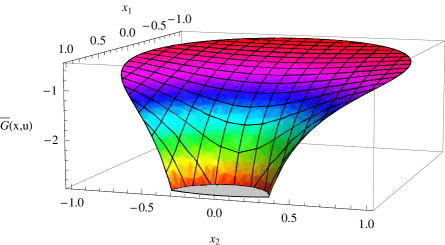
Figure 1: A plot of the screening function for $\epsilon=80$, produced by numerically evaluating and plotting (16) using the standard packages in Mathematica. The axis coordinates in this and subsequent surface plots were chosen to be $x_{1}=xu=x\cos\theta$ and $x_{2}=\pm x\sqrt{1-u^{2}}=\pm x\sin\theta$.

Figure 1 shows a plot of the screening function as a function of the variables $x_{1}=x\cos\theta$ and $x_{2}=x\sin\theta$ in the circular region defined by $0\leq x\leq 1$. For points inside the cavity, $x=rr^{\prime}$ as indicated in (9), so $x_{1}$ and $x_{2}$ are proportional to the spatial coordinates parallel and perpendicular to the $z$-axis, respectively. For a given location $r^{\prime}$ of the source charge, the cavity boundary corresponds to $x=r^{\prime}$ which is at most one, so a plot of the potential inside the cavity may be visualized by truncating the plot in figure 1 to a smaller circular region of radius $r^{\prime}$, and then expanding the plot to fill a region of radius one. The screening function becomes infinite at the point $({x=1},{u=1})$, corresponding to the image point charge referred to in the previous paragraph, but this singularity only shows up in the physical solution when $r^{\prime}=1$, i.e. when the source charge is at the cavity wall.

3 Expansion for Large Values of the Dielectric Constant

Equation (16) provides a concise, exact expression for the screening function, which can be evaluated numerically and also in terms of Appell hypergeometric functions [10]. However, it is of limited use in actual simulations of molecules in which great numbers of these expressions would need to be evaluated. It is therefore useful to look for approximations allowing the use of simpler functions. One such approximation is to recognise that, as we have mentioned, the dielectric constant of water is quite large, so that an expansion good for large values of $\epsilon$ would be useful.

Based on what we have already derived here, there are two ways in which we can obtain a series expansion good for large $\epsilon$. One way is to go back to definition (10) of $G_{n}\left(x,u\right)$ and write it in the form

$$G_{n}\left(x,u\right) = -\,\frac{\epsilon-1}{\epsilon+1}\sum_{l=0}^{\infty}\left[1-\frac{1}{(\epsilon+1)(l-1)}\right]^{-1}x^{l}P_{l}\left(u\right)$$ (17)

$$= -\,\frac{\epsilon-1}{\epsilon+1}\sum_{l=0}^{\infty}\sum_{n=0}^{\infty}\frac{1}{(\epsilon+1)^{n}(l+1)^{n}}\,x^{l}P_{l}\left(u\right).$$

Reversing the order of summation gives us a series in powers of ${1/(\epsilon+1)^{n}}$:

$$\overline{G}\left(x,u,\epsilon\right)=-\,\frac{\epsilon-1}{\epsilon+1}\left(G_{0}\left(x,u\right)+\frac{G_{1}\left(x,u\right)}{\epsilon+1}+\frac{G_{2}\left(x,u\right)}{\left(\epsilon+1\right)^{2}}+\frac{G_{3}\left(x,u\right)}{\left(\epsilon+1\right)^{3}}+\dots\right),$$ (18)

where

$$G_{n}\left(x,u\right)=\sum_{l=0}^{\infty}\frac{x^{l}}{(l+1)^{n}}\,P_{l}\left(u\right).$$ (19)

The other way to get a series is to expand the integral expression (16), noting that

$$x^{-\epsilon/(\epsilon+1)}t^{-1/(\epsilon+1)}=\frac{1}{x}\exp\frac{\ln(x/t)}{\epsilon+1}=\frac{1}{x}\sum_{n=1}^{\infty}\frac{\ln^{n-1}(x/t)}{(k-1)!\left(\epsilon+1\right)^{n-1}}.$$ (20)

This gives the series in (18) again, where this time the coefficients are given by

$$G_{0}\left(x,u\right)=\frac{1}{\sqrt{1-2ux+x^{2}}}$$ (21)

and

$$G_{n}\left(x,u\right)=\frac{1}{(n-1)!}\cdot\frac{1}{x}\int_{0}^{x}\frac{\ln^{n-1}(x/t)}{\sqrt{1-2ut+t^{2}}}\,\rmd t\qquad\mbox{for $n\geq 1$}.$$ (22)

Expression (21) is clearly equivalent to series expression (19) for $n=0$, since the former is the generating function for the Legendre polynomials. It is also possible to show directly that series expression (19) and integral expression (22) are equivalent for $n\geq 0$. Our purpose in deriving these two expressions for $G_{n}\left(x,u\right)$ is that they complement each other: The series is useful for deriving general properties of these coefficients, while the integral is useful for doing actual calculations of them.

To get an idea of what sort of functions may be involved in finding the coefficients $G_{n}\left(x,u\right)$, let us use the series expression to evaluate them in the special case $u=\pm 1$, corresponding to points on the $z$-axis. Since $P_{l}\left(\pm 1\right)=(\pm 1)^{l}$, equation (19) gives

$$G_{n}\left(x,\pm 1\right)=\sum_{l=0}^{\infty}(\pm 1)^{l}\,\frac{x^{l}}{(l+1)^{n}}=\pm\frac{1}{x}\mathrm{Li}_{n}\left[\pm x\right],$$ (23)

where $\mathrm{Li}_{n}$ is the polylogarithm function [11, 12, 13]:

$$\mathrm{Li}_{n}\left[x\right]\equiv\sum_{k=1}^{\infty}\frac{x^{k}}{k^{n}}.$$ (24)

As can be easily seen from this definition, the polylogarithms satisfy a recursion relation,

$$\mathrm{Li}_{n}\left[x\right]=\int_{0}^{x}\frac{\mathrm{Li}_{n-1}\left[t\right]}{t}\,\rmd t.$$ (25)

The polylogarithm for $n=0$ is easily found from definition (24):

$$\mathrm{Li}_{0}\left[x\right]=\frac{x}{1-x},$$ (26)

and those for $n=1,\,2,\,3,\,\ldots$ may be obtained from this function by successive integrations. As a consequence,

$$\mathrm{Li}_{1}\left[x\right]=-\ln(1-x),$$ (27)

while the dilogarithm $\mathrm{Li}_{2}\left[x\right]$, the trilogarithm $\mathrm{Li}_{3}\left[x\right]$, and higher-order polylogarithms cannot be expressed in terms of elementary functions. For any positive integer $n$, $\mathrm{Li}_{n}\left[x\right]$ has a real value for $-\infty<x\leq 1$, but has a branch cut in the complex plane running along the positive real axis from $x=1$ to $\infty$, across which the function has a discontinuous imaginary part.

Like the polylogarithms, the coefficients $G_{n}\left(x,u\right)$ also have a similar recursion relation which follows immediately from series expression (19):

$$G_{n}\left(x,u\right)=\frac{1}{x}\int_{0}^{x}G_{n-1}\left(t,u\right)\,\rmd t,$$ (28)

and in fact the recursion relation for $xG_{n}\left(x,u\right)$ is the same as for $\mathrm{Li}_{n}\left[x\right]$. Equation (28) serves as an alternate way to calculate $G_{n}\left(x,u\right)$ by starting with $G_{0}\left(x,u\right)$ as given by (21).

To calculate $G_{n}\left(x,u\right)$ for specific values of $n$, we can either use integral expression (22) or recursion relation (28); both methods seem to lead to about the same degree of complexity. In both methods we have found it useful to make the change of variable

$$w=\frac{1+t-\sqrt{1-2ut+t^{2}}}{1+u},\quad\mbox{or}\quad t=\frac{w}{1-w}\left(1-\frac{1+u}{2}\,w\right).$$ (29)

In addition, we define the following variables for the sake of convenience,

$$p\equiv\frac{1+x-\sqrt{1-2ux+x^{2}}}{1+u},\qquad q\equiv\frac{1-u}{1+u}.$$ (30)

For physical values of $x$ and $u$, the quantities $p$ and $q$ lie in the range $0\leq p\leq 1$ and $0\leq q<\infty$. The first-order coefficient $G_{1}\left(x,u\right)$ is then easily evaluated using either the integral expression or the recursion relation; both methods lead to the same integral:

$$G_{1}\left(x,u\right) =\frac{1}{x}\int_{0}^{x}\frac{\rmd t}{\sqrt{1-2ut+t^{2}}}=\frac{1}{x}\int_{0}^{p}\frac{\rmd w}{1-w}$$ (31)

$$=-\frac{1}{x}\ln(1-p)=\frac{1}{x}\,\mathrm{Li}_{1}\left[p\right],$$

The higher-order coefficients involve higher-order polylogarithms and become increasingly complicated. A pattern that emerges is that for $n\geq 1$, $xG_{n}\left(x,u\right)$ can be expressed entirely in terms of logarithms and polylogarithms of rational functions of $p$ and $q$. Using transformation (29) on integral (22), along with (30) to eliminate $x$ in the integrand, we obtain

$$xG_{n}\left(x,u\right)=\frac{1}{(n-1)!}\int_{0}^{p}\ln^{n-1}\left[\frac{b(1-w)}{w(1+q-w)}\right]\frac{\rmd w}{1-w},$$ (32)

where $b=p(1+q-p)/(1-p)$. Also, from (28) we obtain a transformed recursion relation,

$$xG_{n}\left(x,u\right)=\frac{1}{x}\int_{0}^{p}tG_{n-1}\left(t,u\right)\left(\frac{1}{w}+\frac{1}{1-w}-\frac{1}{1+q-w}\right)\rmd w,$$ (33)

where $tG_{n-1}\left(t,u\right)$ is assumed to be written in terms of $w$ and $q$. Armed with either of these equations we can evaluate the second-order coefficient without much difficulty. For example, using (33) we have

$$xG_{2}\left(x,u\right)=-\int_{0}^{p}\frac{\ln(1-w)}{w}\,\rmd w-\int_{0}^{p}\frac{\ln(1-w)}{1-w}\,\rmd w+\int_{0}^{p}\frac{\ln(1-w)}{1+q-w}\,\rmd w.$$ (34)

The first integral is just $\mathrm{Li}_{2}\left[p\right]$ and the second one is easily evaluated as $\frac{1}{2}\ln^{2}(1-p)$. The third integral can be found by making the change of variable $w^{\prime}=q/(1+q-w)$; the result is $-\mathrm{Li}_{2}\left[w^{\prime}\right]-\ln(w^{\prime}/q)$ evaluated at the endpoints. The final result is

$$G_{2}\left(x,u\right)=\frac{1}{x}\left\{\mathrm{Li}_{2}\left[p\right]+\mathrm{Li}_{2}\left[\frac{q}{1+q}\right]-\mathrm{Li}_{2}\left[\frac{q}{1-p+q}\right]\right.$$

$$\left.{}+\frac{1}{2}\ln^{2}(1-p)+\frac{1}{2}\ln^{2}(1+q)-\frac{1}{2}\ln^{2}(1-p+q)\right\}.$$ (35)

The third-order coefficient is considerably more complicated, whether we use (32) or (33). We evaluated it using (32), enlisting the aid of Mathematica [14] to find and manipulate the large number of terms and help simplify the expression. In the process we also made use of a number of dilogarithm and trilogarithm identities [12, 13]. Our result is

$$G_{3}\left(x,u\right)=\frac{1}{x}\left\{2\,\mathrm{Li}_{3}\left[p\right]-\mathrm{Li}_{3}\left[\frac{p}{1+q}\right]+\mathrm{Li}_{3}\left[1-p\right]-\mathrm{Li}_{3}\left[\frac{1-p+q}{1+q}\right]\right.$$

$$\left.{}-\mathrm{Li}_{3}\left[\frac{1-p}{1-p+q}\right]+\mathrm{Li}_{3}\left[\frac{1}{1+q}\right]-\mathrm{Li}_{3}\left[\frac{q}{1+q}\right]+\mathrm{Li}_{3}\left[\frac{q}{1-p+q}\right]\right.$$

$$\left.{}-\mathrm{Li}_{3}\left[\frac{pq}{1-p+q}\right]+\ln\frac{(1-p+q)^{2}}{(1-p)(1+q)^{2}}\,\mathrm{Li}_{2}\left[\frac{q}{1+q}\right]\right.$$ (36)

$$\left.{}+\frac{1}{6}\ln^{3}\frac{1-p+q}{(1-p)(1+q)}-\frac{1}{2}\ln\frac{pq}{1+q}\ln^{2}\frac{1-p+q}{(1-p)(1+q)}\right.$$

$$\left.{}-\left[\ln p\ln(1-p)+\ln(1+q)\ln\frac{q}{1+q}\right]\ln\frac{1-p+q}{(1-p)(1+q)}\right\}.$$

One of the complications in writing down the coefficients past first order is that there are many different-looking ways to express each $G_{n}\left(x,u\right)$, due to the numerous identities satisfied by the polylogarithms. In an attempt to be somewhat systematic in our expressions, and also to facilitate the study of their behaviour as well as repeated calculations that would occur in plotting or numerical simulations, we have used these identities where necessary to express the results in a form where the arguments of all polylogarithms are between 0 and 1 inclusive.

As a check on these results, we can look at their behaviour in the limit $u\to 1$, which corresponds to

$$p\to x,\qquad q\to 0.$$ (37)

In (3), the first term in the curly brackets becomes $\mathrm{Li}_{2}\left[x\right]$ while the other terms either become zero or cancel in pairs, so that $G_{2}\left(x,1\right)=\mathrm{Li}_{2}\left[x\right]/x$ as expected from (23). In (3), the first two terms give $\mathrm{Li}_{3}\left[x\right]$ while the rest becomes zero, giving the expected result $G_{3}\left(x,1\right)=\mathrm{Li}_{3}\left[x\right]/x$. The behaviour in the limit $u\to-1$, while correct, is less straightforward; it corresponds to

$$p\to\frac{x}{1+x},\qquad q\to\infty,$$ (38)

and in this limit we obtain

$$G_{2}\left(x,-1\right)=\frac{1}{x}\left\{\mathrm{Li}_{2}\left[\frac{x}{1+x}\right]+\frac{1}{2}\ln^{2}(1+x)\right\},$$ (39)

which reduces to the expected $-\mathrm{Li}_{2}\left[-x\right]/x$ by way of one of the dilog identities. The behaviour of the third-order coefficient is similar.

It should be pointed out that despite the factor of $1/x$ occurring in these expressions, $G_{n}\left(x,u\right)$ is not singular at $x=0$, because the rest of the expression becomes zero there. In fact,

$$G_{n}\left(0,u\right)=1,$$ (40)

as can be seen from series expression (19).

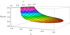
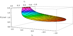
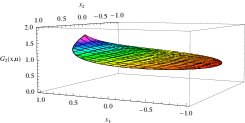
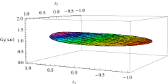
Figure 2: The coefficient functions $G_{0}$ through $G_{3}$.

Figure 2 shows three-dimensional plots of $G_{0}\left(x,\cos\theta\right)$ through $G_{3}\left(x,\cos\theta\right)$ as functions of $x_{1}=x\cos\theta$ and $x_{2}=x\sin\theta$, similarly to figure 1. The zeroth-order coefficient has an inverse first-power singularity at the point $(x=1,u=1)$ corresponding to the image point charge as per the discussion following equation (16), and the first-order coefficient has a logarithmic infinity at that point, while the rest of the coefficients are finite everywhere in the region. Despite the increasing complexity of the expressions as the order becomes higher, their actual behaviour becomes increasingly simple; the plot of the third-order term is comparatively flat. We can in fact obtain bounds on $G_{n}\left(x,u\right)$ in general by noting from integral expression (22) that for any given $x$, the integral will have a maximum value when $u=1$ and a minimum value when $u=-1$. It therefore follows from (23) that for given $x$, the maximum value is $\mathrm{Li}_{n}\left[x\right]/x$ and the minimum value is $-\mathrm{Li}_{n}\left[-x\right]/x$. Since for $0\leq x\leq 1$, $\mathrm{Li}_{n}\left[x\right]/x$ and $-\mathrm{Li}_{n}\left[-x\right]/x$ are strictly increasing and decreasing functions of $x$ respectively, it follows that (for $n\geq 1$) the maximum value over all $x$ and $u$ is $\mathrm{Li}_{n}\left[1\right]=\zeta(n)$, and the minimum value is $-\mathrm{Li}_{n}\left[-1\right]=(1-2^{-n+1})\,\zeta(n)$, where $\zeta(n)$ is the Riemann zeta function:

$$\zeta(n)\equiv\frac{1}{1^{n}}+\frac{1}{2^{n}}+\frac{1}{3^{n}}+\cdots\,.$$ (41)

It follows that

$$(1-2^{-n+1})\,\zeta(n)\leq G_{n}\left(x,u\right)\leq\zeta(n)$$ (42)

for all $x$ and $u$ in the physical region, and for $n\geq 1$. The $n=0$ case is easily treated; the lower bound is $G_{0}\left(1,-1\right)=\frac{1}{2}$. The results are numerically,

$$0.500000 \leq G_{0}\left(x,u\right)<\infty$$

$$0.693147 \leq G_{1}\left(x,u\right)<\infty$$

$$0.822467 \leq G_{2}\left(x,u\right)\leq 1.644934$$ (43)

$$0.901543 \leq G_{3}\left(x,u\right)\leq 1.202057\,.$$

As $n$ becomes large, the lower and upper bounds both approach 1, leading to an increasingly flat plot. The coefficient $G_{n}\left(x,u\right)$ could then be approximated by a simple polynomial, or even a constant, greatly reducing time in computationally intensive problems. However, for problems occurring in practice with large values of the dielectric constant, it may not be necessary to keep very many terms anyway. We will look at the errors due to truncating the series in section 5.

4 Electric Fields

While the potential is useful for calculating the potential energy of the system, one also needs to be able to calculate the force of the various objects upon one another so that the system may evolve from one time step to the next. This in turn requires knowing the electric field due to the charges and the dielectric. Corresponding to the Green’s function $G\left(\mathbf{r};\mathbf{r}^{\prime}\right)$, which is the potential at $\mathbf{r}$ due to a unit point charge at $\mathbf{r^{\prime}}$ in the presence of the dielectric, let us define $\mathbf{E}\left(\mathbf{r};\mathbf{r}^{\prime}\right)$ be the electric field at $\mathbf{r}$ due to a unit point charge at $\mathbf{r^{\prime}}$ in the presence of the dielectric. The electric field is determined from the Green’s function by

$$\mathbf{E}\left(\mathbf{r};\mathbf{r}^{\prime}\right)=-\nabla_{\mathbf{r}}G\left(\mathbf{r};\mathbf{r}^{\prime}\right),$$ (44)

where $\nabla_{\mathbf{r}}$ means the gradient with respect to the vector $\mathbf{r}$, keeping $\mathbf{r^{\prime}}$ constant. Like the potential, the electric field separates into the field to the point charge alone plus the “screening field” due to the polarized dielectric:

$$\mathbf{E}\left(\mathbf{r};\mathbf{r}^{\prime}\right)=\mathbf{E}_{\mathrm{point}}\left(\mathbf{r};\mathbf{r}^{\prime}\right)+\mathbf{E}_{\mathrm{screen}}\left(\mathbf{r};\mathbf{r}^{\prime}\right).$$ (45)

The field $\mathbf{E}_{\mathrm{point}}\left(\mathbf{r};\mathbf{r}^{\prime}\right)$ is the familiar Coulomb field,

$$\mathbf{E}_{\mathrm{point}}\left(\mathbf{r};\mathbf{r}^{\prime}\right)=\frac{\mathbf{r}-\mathbf{r^{\prime}}}{|\mathbf{r}-\mathbf{r^{\prime}}|^{3}}=\frac{(r-r^{\prime}\cos\theta)\,\mathbf{e}_{r}+(r^{\prime}\sin\theta)\,\mathbf{e}_{\theta}}{(r^{2}+r^{\prime 2}-2rr^{\prime}\cos\theta)^{3/2}},$$ (46)

where $\mathbf{e}_{r}$ and $\mathbf{e}_{\theta}$ are unit vectors in the direction of increasing $r$ and $\theta$. In (9) we expressed the screening part of the Green’s function inside and outside of the cavity in terms of a single function $\overline{G}\left(x,u,\epsilon\right)$, which can be thought of as a function of a three-dimensional coordinate $\mathbf{x}$ with spherical coordinates $(x,\theta,\phi)$. Let us define $\overline{\mathbf{E}}\left(x,u,\epsilon\right)$ to be the negative of the gradient of this function:

$$\overline{\mathbf{E}}\left(x,u,\epsilon\right) = -\nabla_{\mathbf{x}}\overline{G}\left(x,u,\epsilon\right)=-\left(\mathbf{e}_{x}\frac{\partial}{\partial x}+\mathbf{e}_{\theta}\frac{1}{x}\,\frac{\partial}{\partial\theta}\right)\overline{G}\left(x,\cos\theta,\epsilon\right)$$ (47)

$$= \left(-\,\mathbf{e}_{x}\frac{\partial}{\partial x}+\mathbf{e}_{\theta}\frac{\sqrt{1-u^{2}}}{x}\,\frac{\partial}{\partial u}\right)\overline{G}\left(x,u,\epsilon\right).$$

Then from (9), the screening field can be written as

$$\mathbf{E}_{\mathrm{screen}}\left(\mathbf{r};\mathbf{r}^{\prime}\right)=\left\{\begin{array}[]{lr}r^{\prime}\,\overline{\mathbf{E}}\left(r^{\prime}r,\cos\theta,\epsilon\right)&\mbox{for $r<1$},\vspace{6pt}\\ \displaystyle\frac{r^{\prime}}{r^{3}}\,\overline{\mathbf{E}}\left(\frac{r^{\prime}}{r},\cos\theta,\epsilon\right)+\frac{1}{r^{2}}\,\overline{G}\left(\frac{r^{\prime}}{r},\cos\theta,\epsilon\right)\mathbf{e}_{r}&\mbox{for $r>1$}.\end{array}\right.$$ (48)

The expansion of $\overline{G}\left(x,u,\epsilon\right)$ in powers of ${1/(1+\epsilon)}$ leads to a corresponding expansion of $\overline{\mathbf{E}}\left(x,u,\epsilon\right)$:

$$\overline{\mathbf{E}}\left(x,u,\epsilon\right)=-\,\frac{\epsilon-1}{\epsilon+1}\left(\mathbf{E}_{0}\left(x,u\right)+\frac{\mathbf{E}_{1}\left(x,u\right)}{\epsilon+1}+\frac{\mathbf{E}_{2}\left(x,u\right)}{\left(\epsilon+1\right)^{2}}+\frac{\mathbf{E}_{3}\left(x,u\right)}{\left(\epsilon+1\right)^{3}}+\dots\right),$$ (49)

where

$$\mathbf{E}_{n}\left(x,u\right)=-\nabla_{\mathbf{x}}G_{n}\left(x,u\right),$$ (50)

The zero-order term is found in a straightforward manner, and is just the Coulomb electric field due to a unit point charge located on the $x$-axis at unit distance from the origin:

$$\mathbf{E}_{0}\left(x,u\right)=\frac{(x-u)\,\mathbf{e}_{x}+\sqrt{1-u^{2}}\,\mathbf{e}_{\theta}}{(1-2ux+x^{2})^{3/2}}.$$ (51)

For the higher orders, we can avoid having to take some of the derivatives of $G_{n}\left(x,u\right)$ explicitly by noticing that if we differentiate both sides of recursion relation (28) with respect to $x$, we obtain

$$\frac{\partial G_{n}}{\partial x}=\frac{1}{x}(G_{n-1}-G_{n})\quad\mbox{for $n\geq 1$}.$$ (52)

The derivative with respect to $u$ is not so easily found, but even it can be simplified. For $n\geq 1$, we found that our expressions for $G_{n}\left(x,u\right)$ were of the form $1/x$ times a function consisting of logarithms and polylogarithms of $p$ and $q$. Therefore, for $n\geq 1$ it is convenient to write

$$\frac{\partial G_{n}}{\partial u}=\frac{1}{x}\,\frac{\partial(xG_{n})}{\partial u}=\frac{1}{x}\left[\frac{\partial p}{\partial u}\,\frac{\partial(xG_{n})}{\partial p}+\frac{\partial q}{\partial u}\,\frac{\partial(xG_{n})}{\partial q}\right].$$ (53)

On the other hand we also know that, again from the recursion relation,

$$G_{n-1}=\frac{\partial(xG_{n})}{\partial x}=\frac{\partial p}{\partial x}\,\frac{\partial(xG_{n})}{\partial p}+\frac{\partial q}{\partial x}\,\frac{\partial(xG_{n})}{\partial q}.$$ (54)

From definitions (30) of $p$ and $q$, the partial derivatives of them with respect to $x$ and $p$ are

$$\begin{array}[]{lr}\displaystyle\frac{\partial p}{\partial x}=\frac{(1-p)^{2}(1+q)}{(1-p)^{2}+q},&\quad\displaystyle\frac{\partial p}{\partial u}=\frac{p^{2}(1-p)(1+q)}{2\left[(1-p)^{2}+q\right]},\vspace{3pt}\\ \displaystyle\frac{\partial q}{\partial x}=0,&\quad\displaystyle\frac{\partial q}{\partial u}=-\,\frac{(1+q)^{2}}{2}.\end{array}$$ (55)

Since $\partial q/\partial x=0$, equation (54) allows us to express $\partial(xG_{n})/\partial x$ in terms of $G_{n-1}$, which can then be used in (53), giving

$$\frac{\partial G_{n}}{\partial u} =\frac{1}{x}\left[\frac{\partial p/\partial u}{\partial p/\partial x}\,G_{n-1}+\frac{\partial q}{\partial u}\,\frac{\partial(xG_{n})}{\partial q}\right]$$ (56)

$$=\frac{1}{x}\left[\frac{p^{2}}{2(1-p)}\,G_{n-1}-\frac{(1+q)^{2}}{2}\,\frac{\partial(xG_{n})}{\partial q}\right]$$

Using these results in (47) along with the fact that $\sqrt{1-u^{2}}=2\sqrt{q}/(1+q)$, we obtain for the $n^{\mathrm{th}}$-order coefficient in the electric field

$$\mathbf{E}_{n}\left(x,u\right)=\frac{1}{x}(G_{n}-G_{n-1})\,\mathbf{e}_{x}+\frac{\sqrt{q}}{x^{2}}\left[\frac{p^{2}}{(1-p)(1+q)}\,G_{n-1}-(1+q)\,\frac{\partial(xG_{n})}{\partial q}\right]\,\mathbf{e}_{\theta}.$$ (57)

so that we only need to take derivatives with respect to $q$. It should be noted that, like $G_{n}\left(x,u\right)$, $\mathbf{E}_{n}\left(x,u\right)$ is not singular at $x=0$ despite the inverse powers of $x$, as they multiply factors which become zero there. In simplifying expressions for the potential and electric field it is sometimes convenient to use the expressions for $x$ and $G_{0}$ in terms of $p$ and $q$:

$$x=\frac{p(1-p+q)}{(1-p)(1+q)},$$ (58)

$$G_{0}\left(x,u\right)=\frac{1}{\sqrt{1-2ux+x^{2}}}=\frac{(1-p)(1+q)}{(1-p)^{2}+q}.$$ (59)

As an example in finding a higher-order coefficient in the electric field, let us evaluate $\mathbf{E}_{1}\left(x,u\right)$. From (31), $xG_{1}=-\ln(1-p)$ which is independent of $q$, so no derivatives have to be taken at all in evaluating (57). After some simplification we obtain

$$\mathbf{E}_{1}\left(x,u\right)=-\,\frac{1}{x^{2}}\left[\frac{p(1-p+q)}{(1-p)^{2}+q}+\ln(1-p)\right]\,\mathbf{e}_{x}+\frac{1}{x^{2}}\,\frac{p^{2}\sqrt{q}}{(1-p)^{2}+q}\,\mathbf{e}_{\theta}.$$ (60)

The $(1-p)^{2}+q$ in the denominator will be recognized as the inverse first-power singularity characteristic of $G_{0}\left(x,u\right)$. As with the potential, the electric field is finite at $x=0$ despite the inverse powers of $x$.

5 Analysis of Errors

In implementing our series expansion (18) for any particular problem, we need to know when we can when we can truncate the series for a given desired degree of accuracy (particularly considering how increasingly complicated the series coefficients become with each subsequent order). Suppose that we have evaluated the series from $n=0$ to $n=N$. The error $e_{N}$ due to ignoring the terms from $N+1$ to infinity is

$$e_{N}=\frac{\epsilon-1}{\epsilon+1}\sum_{n=N+1}^{\infty}\frac{G_{n}\left(x,u\right)}{(\epsilon+1)^{n}}.$$ (61)

The terms in this series are all positive, and the maximum value of $G_{n}\left(x,u\right)$ is $\zeta(n)$ from (42), so

$$e_{N}\leq\frac{\epsilon-1}{\epsilon+1}\sum_{n=N+1}^{\infty}\frac{\zeta(n)}{(\epsilon+1)^{n}}$$ (62)

This sum can be evaluated numerically for any given $\epsilon$ and $N$. For example, using $\epsilon=80$ we find

$$e_{1} \leq 2.468\times 10^{-4}$$

$$e_{2} \leq 2.231\times 10^{-6}$$ (63)

$$e_{3} \leq 2.482\times 10^{-8}.$$

We can also find an upper bound for the fractional error $e_{N}/|\overline{G}\left(x,u,\epsilon\right)|$ by noting that the true value of $|\overline{G}\left(x,u,\epsilon\right)|$ is greater than the $N^{\mathrm{th}}$-order calculated value, and therefore the fractional error will be less than that found by dividing the error by the calculated value. Also, a lower bound over all $x$ and $u$ for the calculated value can be found using the lower bounds for $G_{n}\left(x,u\right)$ in (3). For example, suppose that we have kept only the $n=0$ and $n=1$ terms, again assuming $\epsilon=80$. The maximum error is $e_{1}$ in (5), while the minimum value of $|\overline{G}\left(x,u,\epsilon\right)|$ is at least

$$|\overline{G}\left(x,u,\epsilon\right)|_{\mathrm{min}}=\frac{79}{81}\left(0.5000+\frac{0.6931}{80}\right)=0.4961$$ (65)

and so an upper bound for the fractional error for any $x$ and $u$ is $2.468\times 10^{-4}/0.4961=4.974\times 10^{-4}$. Similarly, for a calculation through second order the fractional error will be less than $4.496\times 10^{-6}$, and for a calculation through third order, less than $5.001\times 10^{-8}$. Of course, the fractional errors will be much smaller than these bounds in regions where $\overline{G}$ is large, even though the error itself do not vary much over the whole region.

6 Use in Molecular Dynamics Simulations

Having obtained our expression for the potential to third order in $\left(1+\epsilon\right)^{-1}$, we now turn to the question of feasibility. That is, to what degree is this calculation useful to those doing large-scale simulations of biological systems?

A cursory objection may be that the computation of special functions as required by this potential for each of the charged objects in a simulation would be intractable, and that it would lead to an inexorable increase in computation time. While certainly true, the problem is not as severe as it first seems.

First, the computation of polylogarithms is very well understood. The Taylor series converges rapidly for arguments in the range $0<x<1$. Moreover, a partial fraction technique exists [15] that converges extremely rapidly. For instance, an evaluation of $\mathrm{Li}_{2}\left[\frac{1}{2}\right]$ converges to within $1\times 10^{-7}$ of the actual value utilizing only 10 divisions.

Second, if the system is of a suitable size, some fields can be calculated using the total charges of extended structures, such as the residues comprising the proteins, rather than the constituent atoms. Since each term in the potential is separately a solution to Laplace’s equation, they each comprise a complete solution. For instance, one could approach a large system by calculating the atomic charges exactly to $O\left[(1+\epsilon)^{-2}\right]$, while using the $G_{2}\left(x,u\right)$ term to calculate screening by using total charge of the protein residues and treating them as point charges.

7 Summary

For the potential of a point charge in a spherical dielectric cavity, the authors have computed integral expressions that lead to a calculable expansion in inverse powers of the relative permittivity. The main feature of this expansion is that the truncated series yields a potential that is accurate over the physical region while remaining a solution to Poisson’s equation at each order. For the case of water, truncating the series to second order leads to a fractional error of no more than $4.5\times 10^{-6}$, and truncating the series to third order leads to a fractional error of no more than $5.0\times 10^{-8}$.

While much of the theoretical groundwork in this article is complete, the feasibility of this model in an actual simulation environment has not been studied. The polylogarithms introduced to describe the series coefficients $G_{n}\left(x,u\right)$ may be computed rapidly and precisely using the partial fraction technique, but it remains to be seen whether the accuracy gains surmount the time lag introduced by having additional terms in the potential. A systematic study of this would need to be done by altering one of the existing molecular dynamics packages such as CHARMM [16] or NAMD [17].

Appendix A Contour Representations

In addition to the methods that we have presented for finding the screening function and the coefficients in the expansion for large $\epsilon$, there are other methods using complex-variable techniques. For example, the second sum in (12) can be found by looking at the special case $u=1$, which can be expressed as a hypergeometric function [9]:

$$\frac{1}{\epsilon+1}\sum_{l=0}^{\infty}\frac{1}{\displaystyle l+\frac{\epsilon}{\epsilon+1}}x^{l}=\frac{1}{\epsilon}\,{}_{2}F_{1}\left[\frac{\epsilon}{\epsilon+1},1;1+\frac{\epsilon}{\epsilon+1};x\right].$$ (66)

The Legendre polynomials can then be brought in by using a contour-integral expression for them,

$$P_{l}\left(u\right)=\frac{1}{2\pi\rmi}\oint\frac{z^{-l}}{\sqrt{1-2uz+z^{2}}}\,\frac{\rmd z}{z},$$ (67)

where the integration is counterclockwise along any path that encircles the origin but does not encircle the branch points of the square root (e.g. a circle of radius less than 1). The sum with the Legendre polynomials can then be expressed in terms of a contour integral:

$$\sum_{l=0}^{\infty}\frac{x^{l}}{\displaystyle l+\frac{\epsilon}{\epsilon+1}}P_{l}\left(u\right) = \frac{1}{2\pi\rmi}\oint\sum_{l=0}^{\infty}\frac{1}{\displaystyle l+\frac{\epsilon}{\epsilon+1}}\frac{\left(z/x\right)^{-l}}{\sqrt{1-2uz+z^{2}}}\,\frac{\rmd z}{z},$$ (68)

$$= \frac{1+\epsilon}{\epsilon}\frac{1}{2\pi\rmi}\oint\frac{{}_{2}F_{1}\left[\frac{\epsilon}{\epsilon+1},1;1+\frac{\epsilon}{\epsilon+1};\frac{x}{z}\right]}{\sqrt{1-2uz+z^{2}}}\,\frac{\rmd z}{z}.$$

The screening function then becomes

$$\overline{G}\left(x,u,\epsilon\right)=-\frac{\epsilon-1}{\epsilon+1}\left[\frac{1}{\sqrt{1-2ux+x^{2}}}+\frac{1}{\epsilon}\frac{1}{2\pi\rmi}\oint\frac{{}_{2}F_{1}\left[\frac{\epsilon}{\epsilon+1},1;1+\frac{\epsilon}{\epsilon+1};\frac{x}{z}\right]}{\sqrt{1-2uz+z^{2}}}\,\frac{\rmd z}{z},\right].$$ (69)

A similar technique can be used in expressing the $n^{\mathrm{th}}$-order coefficient $G_{n}\left(x,u\right)$, using series expression (23) for the case $u=1$ in combination with contour integral (67), giving

$$G_{n}\left(x,u\right)=\frac{1}{x}\frac{1}{2\pi\rmi}\oint\frac{\mathrm{Li}_{n}\left[\displaystyle\frac{x}{z}\right]}{\sqrt{1-2zu+z^{2}}}\,\rmd z.$$ (70)

All of the expressions for the $G_{n}$ listed in the main body of the text may be obtained by directly evaluating this contour expression. In particular, it is easy to derive the recursion relation (28) by direct differentiation of (70).

References

References

- [1] PL Freddolino, AS Arkhipov, SB Larson, A McPherson, and K Schulten. Structure, 14:437–449, 2006.
- [2] T Daren, L Perera, L Li, and L Pedersen. Structure, 7(3):R55–R60, 1999.
- [3] C Niedermeier and P Taven. J. Chem. Phys., 101(1):734, 1994.
- [4] DJ Griffiths. Introduction to Electrodynamics. Benjamin Cummings, 3rd edition, 1999.
- [5] JD Jackson. Classical Electrodynamics. Wiley, 2nd edition, 1975.
- [6] LM Burko. Phys. Rev.E, 65:046618, 2002.
- [7] R Messina. J. Chem. Phys., 117:11062, 2002.
- [8] G Iversen, YI Kharkats, and J Ulstrup. Molec. Phys., 94(2):297–306, 1998.
- [9] Arfken and Weber. Mathematical Methods for Physicists. Harcourt, 5th edition, 2001.
- [10] EW Weisstein. Appell hypergeometric functions. http://mathworld.wolfram.com/AppellHypergeometricFunction.html.
- [11] L Lewin. Polylogarithms and Associated Functions. North Holland, 1981.
- [12] EW Weisstein. Dilogarithm. http://mathworld.wolfram.com/Dilogarithm.html.
- [13] EW Weisstein. Trilogarithm. http://mathworld.wolfram.com/Trilogarithm.html.
- [14] Wolfram Research. Mathematica. Wolfram Research, Inc., Champaign, IL, 5.2 edition, 2005.
- [15] D Cvijovic and J Klinowski. Proc. Amer. Math. Soc., 125(9):2543, 1997.
- [16] B.R. Brooks, R.E. Bruccoleri, D.J. Olafson, D.J. States, S. Swaminathan, and M. Karplus. J. Comput. Chem., 4:187–217, 1983.
- [17] JC Phillips, R Braun, W Wang, J Gumbert, E Tajkhorshid, E Villa, C Chipot, RD Skeel, L Kale, and K Schulten. J. Comput. Chem., 26:1781, 2005.