Galaxy Clusters in the IRAC Dark Field I:
Growth of the red sequence

Abstract

Using three newly identified galaxy clusters at $z\sim 1$ (photometric redshift) we measure the evolution of the galaxies within clusters from high redshift to the present day by studying the growth of the red cluster sequence. The clusters are located in the Spitzer Infrared Array Camera (IRAC) Dark Field, an extremely deep mid-infrared survey near the north ecliptic pole with photometry in 18 total bands from X-ray through far-IR. Two of the candidate clusters are additionally detected as extended emission in matching Chandra data in the survey area allowing us to measure their masses to be $M_{500}=6.2\pm 1.0\times 10^{13}$ and $3.6\pm 1.1\times 10^{13}$ M_⊙. For all three clusters we create a composite color magnitude diagram in rest-frame B-K using our deep HST and Spitzer imaging. By comparing the fraction of low luminosity member galaxies on the composite red sequence with the corresponding population in local clusters at $z=0.1$ taken from the COSMOS survey, we examine the effect of a galaxy’s mass on its evolution. We find a deficit of faint galaxies on the red sequence in our $z\sim 1$ clusters which implies that more massive galaxies have evolved in clusters faster than less massive galaxies, and that the less massive galaxies are still forming stars in clusters such that they have not yet settled onto the red sequence.

1. Introduction

The redshift range from $z=1$ to the present day is a particularly dynamic epoch in the history of groups and clusters as evidenced by the evolution of the morphology-density relation and increasing fraction of blue galaxies with increasing redshift (Capak et al., 2007; Butcher & Oemler, 1984). Interestingly, cluster ellipticals at $z\sim 1$ already have a narrow distribution of red colors (the red cluster sequence (RCS); Blakeslee et al., 2003; van Dokkum et al., 2001). There is some debate about the mechanism by which these cluster galaxies arrive onto the red sequence. It is difficult to distinguish whether these red ellipticals all formed their stars and did their merging at $z>3$, then stopped forming stars when they entered the cluster environment (Ford et al., 2004); or if they are the product of the merging of gas-poor systems which do not produce star formation (van Dokkum, 2005).

We investigate whether the red population is still in the process of forming at $z=1$ or if indeed assembly has already finished at higher redshift by studying the presence of the faint end of the RCS at $z=1$ and comparing it to the present epoch. We measure the ratio of faint to bright RCS galaxies in a sample of three $z\sim 1$ clusters from the IRAC Dark Field (described below). These clusters have the benefit of extremely deep $3.6\,\micron$ data which allows us to study the faint end of the luminosity function at rest frame near-IR, which traces the peak of the spectral energy distribution in galaxies. A confirmed deficit of faint galaxies on the RCS would imply that more massive galaxies have evolved in clusters faster than less massive galaxies. A constant fraction of faint red galaxies between $z=1$ and the present would require a formation mechanism where galaxies of all masses have already joined the red sequence at redshifts higher than one. There is evidence that the faint end of the RCS is not completely in place by z=0.8 (De Lucia et al., 2007; Koyama et al., 2007, and references therein), although at least some clusters at these redshifts appear to have complete RCSs to M*+3.5 (Andreon, 2006).

These questions are ideally addressed with deep infrared surveys of clusters at high redshift. In the last four years deep and wide area surveys in the mid-infrared using the Spitzer Space Telescope have substantially opened a new window on galaxy and star formation at $0<z<3$. Spitzer now routinely produces imaging of large fields to higher resolution and fainter depths than previously possible. IRAC, the mid-infrared camera on-board Spitzer, takes images at 3.6, 4.5, 5.8, and 8.0 µm(Fazio et al., 2004). The shorter wavelengths provide a direct measurement of the stellar content of galaxies at redshifts as high as three. The longer wavelength channels sample emission from polycyclic aromatic hydrocarbons (PAHs) in low redshift galaxies, as well as direct thermal emission from hot dust. The deepest such survey is the dark current calibration field for the mid-infrared camera, commonly known as the “IRAC Dark Field”. These deep mid-IR data are supplemented by additional 14 band photometry including Palomar u’,g’,r’,i’, HST/ACS F814W, MMT $z^{\prime}$, Palomar J, H,& K , Akari 11 & $15\,\micron$, Spitzer MIPS 24 & $70\,\micron$, and Chandra ACIS-I imaging. This extensive, multiwavelength dataset gives us the distinctly unique opportunity to study the development of the red sequence in galaxy clusters at redshift one. The second paper on galaxy clusters in this series will discuss the role of star formation in the evolution of clusters at $z=1$ by examining the Spitzer 24 µm data in conjunction with the morphological information from the HST ACS dataset.

This paper is structured in the following manner. In §2 & §3 we discuss the data and derived photometric redshift determination. Details of the cluster search and cluster properties are presented in §4. In §5 & §6 we present the color magnitude diagrams of the candidate clusters and results of the faint-to bright ratios of red sequence galaxies. In §7 we discuss the implications for the evolution of cluster galaxies. Throughout this paper we use $H_{0}=70$km/s/Mpc, $\Omega_{M}$ = 0.3, $\Omega_{\Lambda}$ = 0.7. With this cosmology, the luminosity distance at z=1 is 6607 Mpc, but the angular diameter distance is a factor of $(1+z)^{2}$ less, or 1652 Mpc. All photometry is quoted in the AB magnitude system.

2. Observations & Data Reduction

2.1. The IRAC Dark Field

The survey region is the IRAC Dark Field, centered at approximately 17h40m +69d. The field is located a few degrees from the north ecliptic pole (NEP) in a region which is darker than the actual pole and is in the Spitzer continuous viewing zone so that it can be observed any time IRAC is powered on for observing. These observing periods are called instrument “campaigns”, and occur roughly once every three to four weeks and last for about a week. Sets of long exposure frames are taken on the Dark Field at least twice during each campaign totaling roughly four hours of integration time per campaign, and these data are used to derive dark current/bias frames for each channel. The dark frames are used by the pipeline in a manner similar to “median sky” calibrations as taken in ground-based near-infrared observing to produce the Basic Calibrated Data (BCD) for all science observations. Each set of dark calibration observations collects roughly two hours of integration time at the longest exposure times in each channel.

The resulting observations are unique in several ways. The Dark Field lies near the lowest possible region of zodiacal background, the primary contributor to the infrared background at these wavelengths, and as such is in the region where the greatest sensitivity can be achieved in the least amount of time. The area was also chosen specifically to be free of bright stars and very extended galaxies, which allows clean imaging to very great depth. The observations are done at many position angles (which are a function of time of observation) leading to a more uniform final psf. Finally, because the calibration data are taken directly after anneals, they are more free of artifacts than ordinary guest observer (GO) observations. Over the course of the mission, the observations have filled in roughly uniformly a region 20′ in diameter. This has created the deepest ever mid-IR survey, exceeding the depth of the deepest planned regular Spitzer surveys over several times their area. Furthermore, this is the only field for which a 5+year baseline of mid-IR periodic observations is expected.

The IRAC data are complemented by imaging data in 14 other bands with facilities including Palomar, MMT, HST, Akari, Spitzer MIPS, and Chandra ACIS-I. Although the entire dark field is $>20\arcmin$ in diameter, because of spacecraft dynamics the central $\sim 15\arcmin$ is significantly deeper and freer of artifacts. Therefore, it is this area which we have matched with the additional observations. The entire dataset will be presented in detail in a future paper (Krick et al, in prep). For completeness we briefly discuss here the Spitzer IRAC, HST ACS, and Chandra ACIS datasets as they are the most critical to this work. All space-based datasets are publicly available through their respective archives.

2.2. Spitzer/IRAC

This work is based on a preliminary combination of 75 hours of IRAC imaging, which is $\approx$30% of the expected depth not including a possible warm mission. Even these 75 hours go well into the confusion limit of IRAC and so the additional exposure time will not add a lot of sensitivity. The Basic Calibrated Data (detector image level) product produced by the Spitzer Science Center was further reduced using a modified version of the pipeline developed for the SWIRE survey (Surace et al., 2005). This pipeline primarily corrects image artifacts and forces the images onto a constant background (necessitated by the continuously changing zodiacal background as seen from Spitzer). The data were coadded onto a regularized 0.6″ grid using the MOPEX software developed by the Spitzer Science Center.

Experiments with DAOPHOT demonstrate that nearly all extragalactic sources are marginally resolved by IRAC, particularly at the shorter wavelengths, and hence point source fitting is inappropriate. Instead, photometry is done using the high spatial resolution ACS data as priors for determining the appropriate aperture shape for extracting the Spitzer data. We do this by first running source detection and photometric extraction on the coadded IRAC images using a matched filter algorithm with image backgrounds determined using the mesh background estimator in SExtractor (Bertin et al. 1995) . This catalog is merged with the HST ACS catalog. For every object in that catalog ,if the object is detected in ACS then we use the ACS shape parameters to determine the elliptical aperture size for the IRAC images. ACS shape parameters are determined by SExtractor on isophotal object profiles after deblending, such that each ACS pixel can only be assigned to one object (or the background). For objects which are not detected in ACS, but which are detected in IRAC, we simply use the original IRAC SExtractor photometry. Because of the larger IRAC beam, we impose a minimum semi-major axis radius of 2″. In all cases aperture corrections are computed individually from PSF’s provided by the Spitzer Science Center based on the aperture sizes and shapes used for photometry.

Final aperture photometry was performed using custom extraction software written in IDL and based on the APER and MASK$\_$ELLIPSE routines with the shape information from SExtractor, from either ACS or IRAC as described above, using local backgrounds. Because we use local backgrounds, the measured fluxes of objects near the confusion limit should have a larger scatter than those non-confused objects, but will on average be the correct flux. This will have the effect of adding scatter to the CMD described below, but will not cause trends of movement for the faint objects in color space. Additionally, this will not effect the photometric redshifts, as it will likely shift all IRAC points up or down, but not relative to each other. The final $95\%$ completeness limit at 3.6 µm is 0.2 $\mu$Jy or 25.7 AB magnitude as calculated from a number count diagram by measuring where the number of observed objects drops below 95% of the expected number of objects, where the expected numbers are calculated by fitting a straight line to the brighter flux number counts.

2.3. HST/ACS

The HST observations consist of 50 orbits with the ACS comprising 25 separate pointings, all with the F814W filter (observed I-band). Within each pointing eight dithered images were taken for cosmic ray rejection and to cover the gap between the two ACS CCDs. The ACS pipeline calacs was used for basic reduction of the images. Special attention was paid to bias subtraction, image registration, and mosaicing. Pipeline bias subtraction was insufficient because it does not measure the bias level individually from each of the four amplifiers used by ACS. We make this correction ourselves by subtracting the mean value of the best fit Gaussian to the background distribution in each quadrant. Due to distortions in the images, registration and mosaicing was performed with a combination of IRAF’s tweakshifts, multidrizzle, and SWarp v.2.16.0 from Terapix. The actual task of mosaicing the final image was complicated by the large image sizes. The single combined mosaic image is 1.7GB and reading in all 200 images (160Mb each) for combination is impossible for most software packages.

The final combined ACS image is $\sim 15\arcmin$ diameter coincident with the deepest part of the IRAC Dark Field and is made with the native $0.05\arcsec$ per pixel resolution. Photometry was performed in a standard manner with SExtractor. The $3\sigma$ detection limit for point sources is $I=28.6(AB)$. The area common to both IRAC and ACS contains $\sim 51,000$ detected sources.

All cluster galaxies are detected in the mid-infrared data, and the ACS data are used as priors for extraction of the mid-IR photometry. Because the cluster galaxies are detected in the optical ACS images, and cluster membership is derived specifically based on the optical data, it is the completeness of the optical data thats sets the fundamental detection limits. Thus our ability to examine the faint end of the cluster (rest frame) K-band luminosity function is ultimately limited by the optical data, not the infrared data.

2.4. Chandra/ACIS-I

The field-of-view of the Chandra ACIS-I is 17′ (for the central four chips) , well-matched to the deepest central area of the Dark Field. As a result, only a single pointing was required. The 100ks observation was broken into three separate observations at different pointing angles to reduce the effect of the gap between chips. The data was reduced using the newest version of the Chandra Interactive Analysis of Observations software (CIAO 4.0). Specific attention was paid to destreaking, bad pixels, and background flares. The task merge_all was then used to combine event files from the three observations into a final event file and image. The final combined Chandra image has $0.5\arcsec$ per pixel resolution. Blind pointing is expected to be 1″. Aperture photometry for extended sources is done manually (see §4.1).

3. Photometric redshifts

The combined IRAC and ACS catalog contains over $50,000$ objects which makes acquisition of spectroscopic redshifts impractical. Even confirmation spectroscopy of red galaxies at $z=1$ in our three candidate clusters will require multiple nights on 8-10m class telescopes. In lieu of spectroscopy we use our extensive multi-wavelength, broad-band catalog to build spectral energy distributions (SEDs) and derive photometric redshifts. These SEDs are fit with template spectra derived from galaxies in the Spitzer wide area infrared survey survey (SWIRE; Polletta et al., 2007). Since the SWIRE templates are based on Spitzer observations we find them the best choice to use as models for this dataset. Photometric redshifts are calculated using Hyperz; a chi-squared minimization fitting program including a correction for Galactic reddening (Bolzonella et al., 2000; Calzetti et al., 2000). We emphasize that in this work photometric redshifts are used only as a first step to find cluster candidates, and not to determine membership within the clusters.

4. Cluster Search

The mid-IR wavelengths of IRAC are well suited to find galaxies at redshift one because the stellar peak of the spectral energy distribution has red-shifted into those bands. We exploit this fact in a search for clusters.

The first step in the search is to combine the spatial information from the 2-D images with photometric redshifts to visually identify clusters of galaxies. We do this by plotting the locations of all galaxies in a certain photometric redshift range on both the optical and IR images to look for clusterings. We step through redshift space in overlapping z=0.2 bins examining each for clusterings. The result of this search is 14 cluster candidates at $0.8<z<1.4$ with average areal densities of 10.3 galaxies with similar redshifts per square arcminute. Next, for each candidate cluster, we examine the redshift distributions of all galaxies within 0.013°of the center ($\sim 375$ Kpc at these redshifts). We choose this radius, at around one third of the virial radius, as the size at which the clustering signal appears to be strongest. The candidate cluster redshift distributions are compared to the average redshift distributions of 50 regions of the same area randomly distributed across the field. After this comparison, three excellent candidate clusters remain with peaks in their redshift distributions which are greater than $2\sigma$ above that of the comparison fields (see Figure 1 & Table 1). In addition the three best candidate clusters show clear over-densities in both the ACS and IRAC images (see Figure 2). While we cannot guarantee that this search is complete without extensive spectroscopy, we are confident that we have found the more massive clusters at redshift one.

In a shallow, large-area IRAC survey Eisenhardt et al. (2008) finds roughly two high-z clusters in an area equivalent to the IRAC dark field. The DEEP2 survey finds seven spectroscopically confirmed groups and clusters with $0.75<z<1.03$ and an upper mass limit of $1\times 10^{13}\hbox{M${}_{\odot}$}$ in a similar area to our survey (Fang et al., 2007). Our finding of three candidate clusters is in agreement with the number of clusters in these other surveys.

Two of the candidate clusters have centers within $1.8\arcmin$ of each other. If clusters were randomly distributed, from Monte Carlo simulations we would expect to find a close pair like this one 2-50% of the time depending on the areal density (here using the IRAC shallow survey and DEEP2 respectively). However, from both hierarchical simulations and cluster surveys we do not expect clusters to be randomly distributed, instead clusters are connected by filaments and are highly correlated even at redshift one(Brodwin et al., 2007). If our two clusters are truly close in all three dimensions then they must lie along a filament. Our photometric redshifts do not allow for the precision needed to know if they indeed are 3-D neighbors.

4.1. X-ray Properties

Two of the three candidate clusters show extended emission in our 100ks Chandra ACIS-I image. This both confirms that they are bound clusters because at these detected luminosities they can only be clusters, and allows us to determine their masses (see Figure 3). We are also able to place a limit on the mass of the third, Chandra undetected, cluster candidate.

X-ray luminosities are obtained by doing aperture photometry on the merged ACIS-I image with the CIAO task dmextract. Aperture sizes were chosen to be 0.9′(0.4Mpc) which fully encompasses all of the excess flux coming from the clusters but avoids neighboring point sources on the Chandra image. Point sources prevent us from using background regions directly adjacent to the clusters, so instead we use the average of 20 background regions taken from empty regions all over the frame. Net counts are 172 $\pm 31$ and 72 $\pm 29$ (Poisson errors) for the clusters respectively. It is possible that the brighter cluster (on the right in Figure 3) is contaminated by a point source which is effecting this count rate, however with such low number of photons we have not attempted to separate this possible point source from the cluster and background.

Taking the count rate from the image, we use the Portable Interactive Multi-Mission Simulator (PIMMS v 3.9d) to derive a flux assuming a thermal bremsstrahlung model with $4\times 10^{20}$cm^-2 of Galactic NH (measured for the location of this field), and a temperature of 5KeV. This temperature is chosen randomly and is calculated more accurately in the following iterative process. Once we have calculated a flux and luminosity of the clusters, we use a combination of the Maughan et al. (2006) and Vikhlinin et al. (2002) $L_{x}-T$ relation based on Chandra and XMM data on 22 clusters with $z>0.4$ to derive a more realistic temperature. We then go back and use this new temperature to re-calculate the X-ray flux and luminosity. The two clusters with detections have luminosities of $3.6\pm 0.6\times 10^{43}$ and $1.6\pm 0.7\times 10^{43}$ erg/s in the 0.5-2 Kev band.

4.2. Mass

To derive the mass from the X-ray luminosity for the two detected clusters, we use the Maughan (2007) $L_{x}-M_{500}$ relation based on 34 clusters with $0.5<z<1.3$. Derived masses are $M_{500}=6.2\pm 1.4\times 10^{13}$ and $3.6\pm 1.4\times 10^{13}$ M_⊙. Since the second cluster is a very low count detection, we take this mass to be the upper limit to the mass of the third, Chandra undetected, cluster. Quoted errors only represent error in the measurements, including uncertainties in redshift, but do not take into account error in the models and should therefore be taken as optimistic.

There is some evidence that using X-ray luminosities to estimate mass is unreliable at high redshift in the sense that higher redshift clusters have lower x-ray luminosities for a given mass (Lubin et al., 2004; Fang et al., 2007). The DEEP2 survey of the aforementioned seven clusters at $0.75<z<1.0$ detect none of their clusters in a 200ks Chandra image (Fang et al., 2007). A possible reason for this is that clusters are not virialized at higher redshifts, an assumption which is necessary to use the cluster hot gas to measure mass. Alternatively, Andreon et al. (2008) have proposed that there are no underluminous X-ray clusters and that previous work has either not properly measured cluster mass via velocity dispersion, or have not correctly interpreted their X-ray observations. If high-z clusters are underluminous in X-rays then there are two relevant implications: 1) our high-z clusters have true masses which are higher than measured from their Chandra luminosities, and 2) this leaves open the possibility that the Chandra undetected cluster is a true cluster with mass larger than the limit afforded by the current non-detection. The resolution of this issue is beyond the scope of this paper.

As a check of cluster mass we have considered using the SDSS relation of optical richness to the weak lensing mass of clusters at low redshifts (Johnston et al., 2007). This relies on multiple assumptions and relations such as that between the number of red sequence galaxies inside of $1h^{-1}$Mpc with luminosities greater than $0.4L^{*}$ and $r_{200}$, the radius at which the cluster is 200 times the critical density of the universe (Hansen et al., 2007) . Furthermore one has to then use the derived value of $r_{200}$ with the weak-lensing relation to arrive at $M_{200}$. To our knowledge none of these relations have been tested at high redshifts and we therefore choose not to make this calculation.

The measured mass of these clusters is consistent with the masses of the, to date, roughly 35 published groups and clusters with confirmed redshifts above 0.9 (Stanford et al., 1997; Ebeling et al., 2001; Stanford et al., 2001, 2002; Blanton et al., 2003; Rosati et al., 2004; Margoniner et al., 2005; Mullis et al., 2005; Siemiginowska et al., 2005; Elston et al., 2006; Stanford et al., 2006; Fang et al., 2007; Finoguenov et al., 2007; Eisenhardt et al., 2008). About two thirds of these clusters are detected in multi-wavelength surveys such as DEEP2, COSMOS, and the IRAC shallow survey and have an average mass of $3.8\times 10^{13}\hbox{M${}_{\odot}$}$. The rest are detected in serendipitous X-ray imaging or are targeted for their location around radio galaxies. These other clusters all have higher masses ($>1E14\hbox{M${}_{\odot}$}$) which is consistent with it being easier to detect high-mass clusters in the X-ray and high mass clusters around radio galaxies. Overall we expect from hierarchical formation that clusters at $z=1$ should be less massive than clusters at $z=0$.

5. Color Magnitude Diagrams

Most galaxies in clusters are ellipticals that have approximately the same red color regardless of magnitude and therefore form a red cluster sequence (RCS) in a color magnitude diagram (CMD), as long as the color is chosen to span the 4000 Å break. Past studies with HST have shown that the RCS is in place at least by redshift one, if not before (Blakeslee et al., 2003; van Dokkum et al., 2001). We choose to make CMDs of the dark field clusters with ACS F814W and Spitzer $3.6\,\micron$. At $z\sim 1$ this corresponds to rest-frame B-K which does span the Balmer break. We generate a composite color magnitude diagram for all three clusters including all galaxies within 0.017°($\sim 500$ Kpc) of the candidate cluster centers (Figure 4). The upper axis is plotted as absolute K-band magnitude in order to compare to a low redshift sample. Because $3.6\,\micron$ at $z=1$ corresponds to K-band at $z\simeq 0.1$, we do not have to apply a K-correction to the data, which avoids a large set of uncertainties. We do make a correction for the redshifting of the bandpass and a correction for the luminosity evolution of galaxies over time taken from the stellar evolution models of Bruzual & Charlot (2003). The color of RCS is consistent with the predicted colors from simple stellar populations with a single burst of star formation above z=3 and a Salpeter initial mass function (Bruzual & Charlot, 2003).

Without benefit of spectroscopy we determine membership based on location in the CMD. Pinpointing the location of the RCS becomes easier when using a composite CMD from three clusters. To determine the location of the RCS, the bright end of the composite red sequence ($[3.6]<22.5$) is fit with a biweight function (Beers et al., 1990) where the slope is fixed to -0.12 (to match the low redshift slope below). The faint end is left out of the fit because of the larger amount of contamination by field galaxies. Members are taken to be those galaxies which lie within $\pm 0.5$ mag of the RCS. We determine the significance of the existence of a red sequence in our CMD by doing a monte carlo calculation with 100 realizations of the CMDs of randomly selected galaxies in the dataset. From this calculation we find that the number of galaxies on the true RCS is significant compared to random galaxies at the $6.7\sigma$ level. The histogram of member galaxies in the composite cluster is shown in Figure 4.

Although the RCS is mainly composed of cluster galaxies at a particular redshift, there will be some fore- and back-ground galaxies that will contaminate the membership count. We statistically subtract fore-and back-ground galaxies within the measured RCS. The number of contaminating galaxies is calculated by counting the average number of galaxies from 50 random regions of the same size as the clusters which have colors consistent with the measured RCS. The average number of contaminating galaxies within a cluster area (0.017°) and their standard deviation are $40.3\pm 7.3$ and $16.9\pm 8.0$ respectively for the magnitude bins used below ( $-20<M_{k}<-18$ and $-22<M_{k}<-20$). After this subtraction the number of member galaxies remaining in each cluster is a few to none in the faint bin, and about twenty each in the bright bin.

We create CMDs for a comparison sample of low redshift clusters using the same process on publically available B- and K- band data from the Cosmic Evolution Survey (COSMOS; Capak et al., 2007). From COSMOS we use four X-ray confirmed clusters with average $0.09<z<0.12$ (Finoguenov et al., 2007, Id’s 42, 58, 113, 140). These clusters have an average mass of $M_{500}=1.1\times 10^{13}\hbox{M${}_{\odot}$}$ as determined from the X-ray temperature. Figure 5 shows both the CMD of the composite COSMOS data from four clusters and the K-band distribution of RCS member galaxies including a statistical correction for fore- and back-ground galaxies taken from neighboring COSMOS regions.

This comparison sample is not ideal since these low redshift clusters are roughly the same mass as the high-z clusters, and we expect clusters to hierarchically gain mass over time through the infall of other groups and clusters. Unfortunately, to our knowledge, there is no sufficiently deep near-IR imaging on local $\sim 10^{\{}14\}$M_⊙clusters. While it is possible that more massive clusters will have fewer faint red galaxies than a less massive cluster due to merging, we do not expect this to be a large effect. Deep, wide-field, near-IR imaging of local clusters is required to study this effect in detail.

The CMD’s from the two samples have clear differences. Despite our ultradeep data, the distribution of the $z=0.1$ galaxies extends to fainter magnitudes than that for the clusters at $z=1$ (thanks to the approximately four magnitudes of surface brightness extinction). We plot the deeper low redshift data to $M_{K}=-14$, whereas for the high redshift dark field clusters we can only plot a smaller range of magnitudes extending to $M_{k}=-18$. Everything fainter than that is below our $5\sigma$ detection threshold, so we are unable to compare that magnitude range with the lower redshift clusters.

6. Results

We investigate the evolution of the fraction of faint galaxies on the red sequence from redshift one to the present. To make the comparison between the two different redshift samples, we choose a rest-frame K-band absolute magnitude range which is both brighter than the $5\sigma$ detection threshold for both datasets, and not too far towards the bright end of the luminosity function that extremely small number statistics would effect the measurement. We divide the resulting magnitude range into two bins which are two magnitudes wide; $-20<M_{k}<-18$ (faint bin), and $-22<M_{k}<-20$ (bright bin).

The quantity we want to measure is the amount of faint galaxies on the RCS at $z=1$ compared to the present epoch as an evolutionary measure of the build-up of the red sequence. This is calculated as the ratio of faint RCS galaxies to bright RCS galaxies. This faint-to-bright ratio is shown explicitly for both cluster samples in Figure 6 and can also be seen by comparing Figures 4 & 5. We find that the relative number of faint galaxies on average in clusters at redshift one is less than in the average cluster at redshift 0.1 at the $3\sigma$ level.

The major sources of error in this work are the background measurement of field galaxies, the area over which cluster membership is determined, the possibility that the third cluster is a chance projection, and the size of the magnitude bins. Recall that completeness in the IRAC data is not a limiting factor to this measurement because we use ACS source locations and shapes as a prior for doing IRAC photometry. To quantify the error originating from the field galaxy subtraction, error bars on Figure 6 show one standard deviation on the background measurement propagated to the ratio of faint to bright number of galaxies.

To estimate the effect of changing the area over which cluster members are counted we re-calculate the faint-to-bright ratio using a radius which is 50% larger than the original radius (2.25 times the area). The original radius was chosen as a compromise between the relative physical sizes of the implied area around the low redshift and high redshift clusters. For reference the original 500 Kpc radius circle is shown on the IRAC images in Figure 2. The new, larger radius, ratios are shown as stars in Figure 6. The effect of changing radius is negligible.

We examine the possibility that the third cluster is a chance projection, not a cluster, and therefore contaminating this measurement. Spectroscopy is the best way to confirm that it is a cluster. Without spectroscopy, we re-calculate the ratios without the third cluster, using just the two X-ray detected clusters. The same trend of the bright galaxies far outnumbering the faint galaxies on the red sequence at z=1 is recovered, albeit with a larger noise contribution. Additionally, we test that any two clusters are dominating the signal by removing one cluster from the measurement in turn. When we recalculate ratios each time the significance of the signal goes down. From this we conclude that all three clusters are contributing to the signal.

Lastly, we consider the possibility that the four magnitude range used is too large in that it goes too close to the very uncertain bright end of the luminosity function of the z=0.1 clusters, and too far into a regime where photometry is confused at the faint end of the luminosity function in the z=1.0 clusters. To test our results, we re-calculate the ratios with 1.5 magnitude wide bins centered at $M_{K}=-20$. We find, again, the same trend of faint galaxies disappearing from the red sequence population at high redshift.

There is a clear deficit of faint galaxies on the red sequence at z=1 compared to the current epoch when taking into account possible sources of error.

7. Discussion

We find that there are fewer faint red cluster galaxies at high redshift than low redshift in comparison to the number of bright red galaxies. There are two possible explanations for this. There could be overall less faint cluster galaxies at z=1 at all colors than the present epoch, or the faint end of the red sequence is not yet in place, and instead those galaxies which will fill the faint end at z=0, are still forming stars at higher redshifts.

The first explanation, that there are overall, at all colors, fewer faint galaxies at z=1 than at z=0, goes directly against the theory of hierarchical formation. We expect that clusters at higher redshifts will have more faint galaxies than today, and that over time the faint galaxies will merge into brighter, more massive galaxies. This will have the effect of clusters at higher redshifts having steeper faint end slopes of the luminosity function than today’s flatter slopes, or exactly the opposite trend of what would be suggested if overall there were less faint galaxies at $z=1$. While we do not think this is a likely solution, it is interesting that in a simulation of cluster luminosity functions, Khochfar et al. (2007) find a slight trend that the faint end slope of clusters does steepen from redshift 1 to 0, whereas overall they find the hierarchical formation trend of flattening slope from z=6 to 0. This is probably due to noise in their calculation. It would be nice to know how the overall faint end slope of clusters is evolving from z=1 to 0, however we do not have a large enough sample to attack this problem.

It is more likely that the deficit of faint red galaxies at high z is due to the fact that those faint galaxies are still forming stars, and so have bluer colors at those redshifts. This implies that a) bright, massive galaxies have already shut off their star formation in clusters by z=1, and b) faint, less massive galaxies are still forming stars in clusters at z=1. We know that clusters exhibit red sequences at higher z, so it is not new that massive galaxies have already undergone some process, excited by the cluster environment, which keeps them from forming stars, and lands them on the red sequence. This is further evidence for the popular theory of ’downsizing’, in which the more massive galaxies evolve first. However, all galaxies in clusters do not follow the same evolutionary processes, instead evolution from the blue cloud to the red sequence seems to be mass dependent. Whatever process stops star formation in clusters appears has not yet happened at z=1 to the less massive galaxies. Those galaxies are still being allowed to form enough stars to stay off of the red sequence. The red population of clusters is not yet fully in place by z=1.

We do not compare the specific values of faint-to-bright ratios of this work with those in the literature as different wavelengths, areas, and definitions of faint and bright are used. However the trend for a deficit of faint galaxies at high redshifts is in agreement with the works of De Lucia et al. (2007); Gilbank et al. (2008); Stott et al. (2007) and Koyama et al. (2007), but in contrast to Andreon (2007). The cause of the difference is unclear, but we note that we use a much redder, wider filter set at high redshifts (rest-frame B-K) than Andreon (2007) (rest-frame u-g). We also compare with the same rest-frame color at low redshift without applying a k-correction.

Future work in this field requires a large enough sample of confirmed clusters at high-z with consistent observations well below $M^{*}$ to be able to split the sample on cluster properties. There are hints that the faint-to-bright ratios are cluster mass or richness dependent, but the literature shows contradictory trends for these effects likely due to the small samples used to date (Gilbank et al., 2008; De Lucia et al., 2007). With this evidence for ongoing star formation in clusters at z=1, in paper two of this series we will examine the star formation rates and morphologies of the cluster galaxies using deep SPITZER MIPS $24\,\micron$ and HST ACS F814W data. Additionally as the community continues to build a larger sample of high redshift clusters we will be able to study their properties, in particular their suitability for dark energy number count surveys (Wang et al., 2004).

Table 1Cluster Characteristics

Cluster	ra	dec	$N_{gals}$	z${}_{peak}\tablenotemark{a}$	Lx (0.5-2.0 Kev)	M500
	J2000 (deg)	J2000 (deg)	$r<500Kpc$		$1\times 10^{43}$erg/s	$1\times 10^{13}\hbox{M${}_{\odot}$}$
1	264.68160	69.04481	215	$1.0\pm 0.1$	$3.6\pm 0.6$	$6.2\pm 1.4$
2	264.89228	69.06851	255	$1.0\pm 0.1$	$1.6\pm 0.7$	$3.6\pm 1.4$
3	264.83102	69.09031	241	$1.0\pm 0.2$	$\leq 1.6\pm 0.7$	$\leq 3.6\pm 1.1$

Figure 1.— Redshift distributions of the three candidate clusters. The solid histogram shows the redshifts for all galaxies within $\sim 375$ Kpc of the cluster centers. The dotted line shows the average redshift distribution of the field galaxy population measured in regions with the same area. These distributions are based on photometric redshifts.

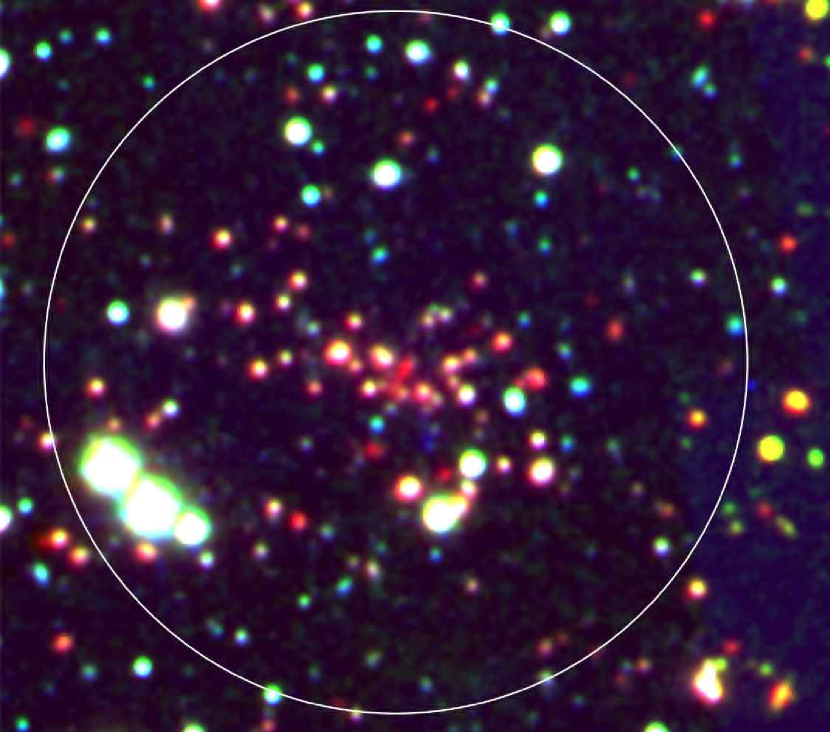
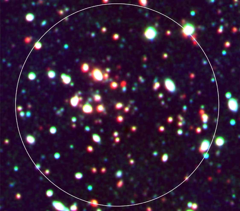
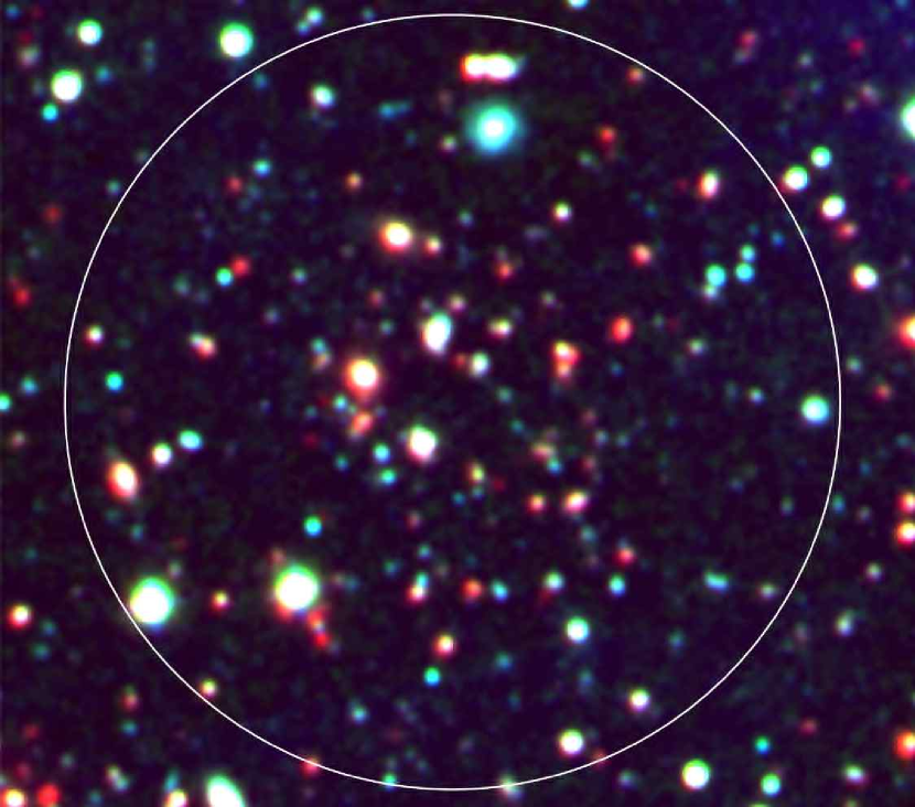
Figure 2.— Color composite images of candidate clusters from ACS F814 (blue), MMT $z^{\prime}$ (green), and IRAC $3.6\,\micron$ (red) data all smoothed to the resolution of the IRAC data. The circle shows the 0.017°(500Kpc) radius used to count the number of galaxies on the red sequence.

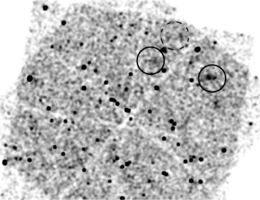
Figure 3.— Chandra ACIS-I 0.3 - 7kev image of extended emission in the field. The two detected clusters are encircled with a 500Kpc radius circle. The third, undetected cluster location is shown with a dashed line circle. The detected cluster on the right has a higher count rate and therefore a higher mass. Specifically the extended emission is associated with the center of the cluster and not with the stars in the bottom left of Figure 2.The extended emission just below the cluster on the right corresponds to a cluster at z_phot=0.25, and is not discussed in this paper.

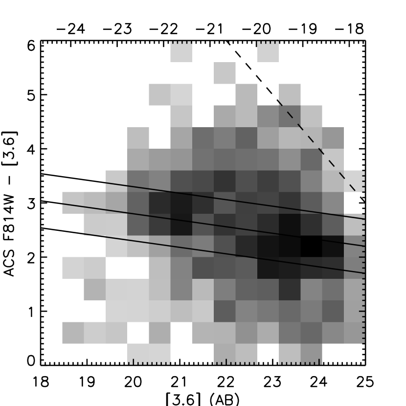
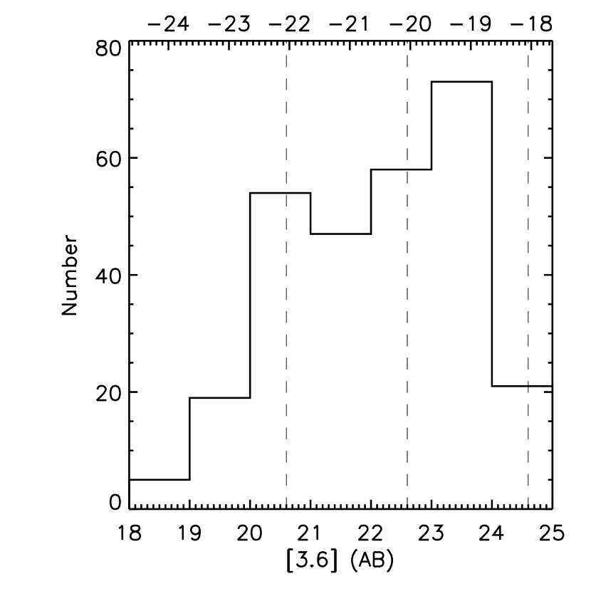
Figure 4.— Left: Color magnitude diagram of all 711 galaxies within 500 Kpc of the centers of the three clusters at z=1 from the IRAC dark field. Greyscale indicates the density of galaxies within each bin. Lines represent the RCS $\pm 0.5$mag. The top scale is absolute rest frame K-band magnitude. The dashed line shows the $5\sigma$ detection limit of the ACS data which does not come close to our fitted RCS. The CMD is plotted only to magnitudes well brighter than the measured 95% completeness limit of the IRAC data. Right: Distribution of galaxies along the red sequence for the composite cluster at z=1. Dashed lines delineate the faint and bright magnitude bins used in the analysis.

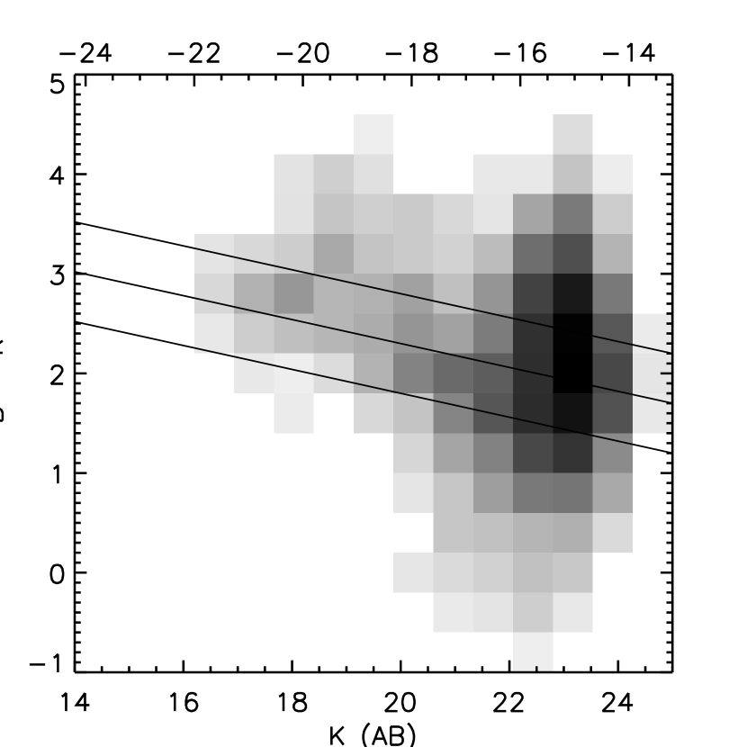
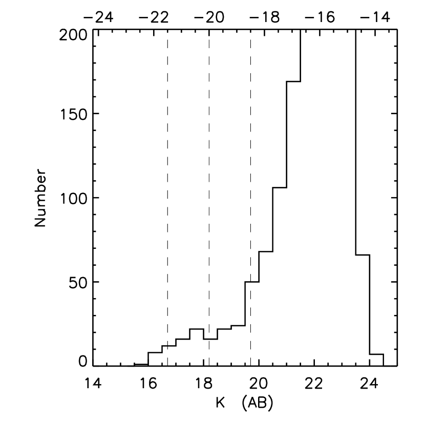
Figure 5.— Color magnitude diagram and K-band distribution for the composite COSMOS cluster at z=0.1. Lines have the same meaning as Figure 4. For clarity this CMD only includes those galaxies with photometric redshifts in the range of the clusters, however the actual measurement is made in the exact same way as for the clusters at $z=1$ which is to use the RCS minus a statistical background for membership information.

Figure 6.— Ratio of faint-to-bright galaxies on the red sequence in both the samples at high and low z. Squares represent background subtracted numbers of member galaxies on the red sequence measured inside of a 500 KPC radius. Stars show the same measurement for a 750 Kpc radius. Error bars are only shown on the 500 Kpc points and represent error in the background measurement.

References

- Andreon (2006) Andreon, S. 2006, A&A, 448, 447
- Andreon (2007) —. 2007, ArXiv e-prints, 710
- Andreon et al. (2008) Andreon, S., de Propris, R., Puddu, E., Giordano, L., & Quintana, H. 2008, MNRAS, 383, 102
- Beers et al. (1990) Beers, T. C., Flynn, K., & Gebhardt, K. 1990, AJ, 100, 32
- Blakeslee et al. (2003) Blakeslee, J. P. et al. 2003, ApJ, 596, L143
- Blanton et al. (2003) Blanton, E. L., Gregg, M. D., Helfand, D. J., Becker, R. H., & White, R. L. 2003, AJ, 125, 1635
- Bolzonella et al. (2000) Bolzonella, M., Miralles, J.-M., & Pelló, R. 2000, A&A, 363, 476
- Brodwin et al. (2007) Brodwin, M., Gonzalez, A. H., Moustakas, L. A., Eisenhardt, P. R., Stanford, S. A., Stern, D., & Brown, M. J. I. 2007, ApJ, 671, L93
- Bruzual & Charlot (2003) Bruzual, G., & Charlot, S. 2003, MNRAS, 344, 1000
- Butcher & Oemler (1984) Butcher, H., & Oemler, A. 1984, ApJ, 285, 426
- Calzetti et al. (2000) Calzetti, D., Armus, L., Bohlin, R. C., Kinney, A. L., Koornneef, J., & Storchi-Bergmann, T. 2000, ApJ, 533, 682
- Capak et al. (2007) Capak, P. et al. 2007, ApJS, 172, 99
- De Lucia et al. (2007) De Lucia, G. et al. 2007, MNRAS, 374, 809
- Ebeling et al. (2001) Ebeling, H., Jones, L. R., Fairley, B. W., Perlman, E., Scharf, C., & Horner, D. 2001, ApJ, 548, L23
- Eisenhardt et al. (2008) Eisenhardt, P. R. M. et al. 2008, ArXiv e-prints, 804
- Elston et al. (2006) Elston, R. J. et al. 2006, ApJ, 639, 816
- Fang et al. (2007) Fang, T. et al. 2007, ApJ, 660, L27
- Fazio et al. (2004) Fazio, G. G. et al. 2004, ApJS, 154, 10
- Finoguenov et al. (2007) Finoguenov, A. et al. 2007, ApJS, 172, 182
- Ford et al. (2004) Ford, H. et al. 2004, in Astrophysics and Space Science Library, Vol. 319, Penetrating Bars Through Masks of Cosmic Dust, ed. D. L. Block, I. Puerari, K. C. Freeman, R. Groess, & E. K. Block, 459–+
- Gilbank et al. (2008) Gilbank, D. G., Yee, H. K. C., Ellingson, E., Gladders, M. D., Loh, Y.-S., Barrientos, L. F., & Barkhouse, W. A. 2008, ApJ, 673, 742
- Hansen et al. (2007) Hansen, S. M., Sheldon, E. S., Wechsler, R. H., & Koester, B. P. 2007, ArXiv e-prints, 710
- Johnston et al. (2007) Johnston, D. E. et al. 2007, ArXiv e-prints, 709
- Khochfar et al. (2007) Khochfar, S., Silk, J., Windhorst, R. A., & Ryan, Jr., R. E. 2007, ApJ, 668, L115
- Koyama et al. (2007) Koyama, Y., Kodama, T., Tanaka, M., Shimasaku, K., & Okamura, S. 2007, MNRAS, 382, 1719
- Lubin et al. (2004) Lubin, L. M., Mulchaey, J. S., & Postman, M. 2004, ApJ, 601, L9
- Margoniner et al. (2005) Margoniner, V. E., Lubin, L. M., Wittman, D. M., & Squires, G. K. 2005, AJ, 129, 20
- Maughan (2007) Maughan, B. J. 2007, ApJ, 668, 772
- Maughan et al. (2006) Maughan, B. J., Jones, L. R., Ebeling, H., & Scharf, C. 2006, MNRAS, 365, 509
- Mullis et al. (2005) Mullis, C. R., Rosati, P., Lamer, G., Böhringer, H., Schwope, A., Schuecker, P., & Fassbender, R. 2005, ApJ, 623, L85
- Polletta et al. (2007) Polletta, M. et al. 2007, ApJ, 663, 81
- Rosati et al. (2004) Rosati, P. et al. 2004, AJ, 127, 230
- Siemiginowska et al. (2005) Siemiginowska, A., Cheung, C. C., LaMassa, S., Burke, D. J., Aldcroft, T. L., Bechtold, J., Elvis, M., & Worrall, D. M. 2005, ApJ, 632, 110
- Stanford et al. (1997) Stanford, S. A., Elston, R., Eisenhardt, P. R., Spinrad, H., Stern, D., & Dey, A. 1997, AJ, 114, 2232
- Stanford et al. (2002) Stanford, S. A., Holden, B., Rosati, P., Eisenhardt, P. R., Stern, D., Squires, G., & Spinrad, H. 2002, AJ, 123, 619
- Stanford et al. (2001) Stanford, S. A., Holden, B., Rosati, P., Tozzi, P., Borgani, S., Eisenhardt, P. R., & Spinrad, H. 2001, ApJ, 552, 504
- Stanford et al. (2006) Stanford, S. A. et al. 2006, ApJ, 646, L13
- Stott et al. (2007) Stott, J. P., Smail, I., Edge, A. C., Ebeling, H., Smith, G. P., Kneib, J.-P., & Pimbblet, K. A. 2007, ApJ, 661, 95
- Surace et al. (2005) Surace, J. A., Shupe, D. L., Fang, F., Evans, T., Alexov, A., Frayer, D., Lonsdale, C. J., & SWIRE Team. 2005, in Bulletin of the American Astronomical Society, Vol. 37, Bulletin of the American Astronomical Society, 1246–+
- van Dokkum (2005) van Dokkum, P. G. 2005, AJ, 130, 2647
- van Dokkum et al. (2001) van Dokkum, P. G., Stanford, S. A., Holden, B. P., Eisenhardt, P. R., Dickinson, M., & Elston, R. 2001, ApJ, 552, L101
- Vikhlinin et al. (2002) Vikhlinin, A., VanSpeybroeck, L., Markevitch, M., Forman, W. R., & Grego, L. 2002, ApJ, 578, L107
- Wang et al. (2004) Wang, S., Khoury, J., Haiman, Z., & May, M. 2004, Phys. Rev. D, 70, 123008