Landau-Zener tunnelling in dissipative circuit QED

Abstract

We investigate the influence of temperature and dissipation on the Landau-Zener transition probability in circuit QED. Dissipation is modelled by coupling the transmission line to a bath of harmonic oscillators, and the reduced density operator is treated within Bloch-Redfield theory. A phase-space representation allows an efficient numerical implementation of the resulting master equation. It provides reliable results which are valid even for rather low temperatures. We find that the spin-flip probability as a function of temperature and dissipation strength exhibits a non-monotonic behaviour. Our numerical results are complemented by analytical solutions for zero temperature and for vanishing dissipation strength.

1 Introduction

The demonstration of coherent quantum dynamics in superconducting flux and charge qubits [1, 2, 3] represents a major step towards a solid-state implementation of a quantum computer. Manipulation and readout of a qubit can be achieved by a controlled interaction with an electromagnetic circuit. For charge qubits implemented with Cooper-pair boxes, this can be established either by a capacitive coupling to a transmission line [4, 5] or an oscillating circuit [6, 7] which can be modelled as a harmonic oscillator. The corresponding qubit-oscillator model also plays a role for the description of a flux qubit that couples inductively to an embracing dc SQUID [8]. These setups represent solid-state realizations of a two-level atom in an optical cavity [9, 10]. As compared to optical realizations, most solid-state implementations are characterised by a much larger ratio between qubit-oscillator coupling and oscillator linewidth [5].

Circuit QED experiments have already demonstrated quantum coherent dynamics [11], measurements with low backaction [7, 12], and the creation of entanglement between two qubits in a cavity [13, 14]. A further crucial prerequisite for a working quantum computer is quantum state preparation, i.e. the initialisation of the qubits. It has been suggested to achieve this goal by switching a control parameter through an avoided crossing with an intermediate velocity, such that the resulting Landau-Zener transition is neither in the adiabatic nor in the diabatic limit [15, 16]. Then the avoided crossing effectively acts like a beam splitter.

The physics of Landau-Zener tunnelling is also of relevance for adiabatic quantum computation which relies on the time evolution of the ground state of a quantum system of a slowly time-dependent Hamiltonian [17]. In this scheme, a relevant source of errors are Landau-Zener transitions at avoided crossings between adiabatic energy levels. For an isolated two-level system, the corresponding transition probability has been derived in the classic works by Landau, Zener, and Stueckelberg [18, 19, 20]. When the qubit is coupled to a heat bath, this probability may change significantly. However, there exist also system-bath interactions for which the transition probability at zero temperature surprisingly is not affected at all by the coupling to a harmonic-oscillator bath [21] or a spin bath [22, 23]. For a heat bath with Ohmic spectral density, the transition probability at high temperatures is bath-independent as well [24, 25, 26, 27, 28]. The same holds true for the coupling to a classical noise source [29, 30, 31].

With this work we study finite temperature Landau-Zener transitions of a qubit that couples via a harmonic oscillator to a heat bath. For the qubit itself, this represents a case of a structured heat bath, because owing to its linearity, the oscillator plus the bath can be considered as an effective bath with a peaked spectral density [32, 33, 34, 35, 36, 37, 38, 39, 40] for which we provide results for the dissipative Landau-Zener problem for finite temperatures. In doing so, we restrain from eliminating this extra oscillator degree of freedom because in the present context, the oscillator dynamics is of experimental interest as well. The organisation of the work is as follows. In section 2, we introduce the qubit-oscillator-bath model and its treatment within Bloch-Redfield theory. Section 3 is devoted to Landau-Zener transitions for a thermal initial state, while in section 4, we investigate dissipative transitions. Details of the derivation of the quantum master equation and its numerical treatment are deferred to the appendices.

2 Model and master equation

2.1 Landau-Zener dynamics in circuit QED

Circuit QED involves a Cooper pair box that couples capacitively to a transmission line which is described as a harmonic oscillator [5]. The Cooper pair box is formed by a dc SQUID such that the effective Josephson energy ${E_{\rm J}}=E_{\mathrm{J}}^{0}\cos(\pi\Phi/\Phi_{0})$ can be tuned via an external flux $\Phi$, where $\Phi_{0}$ denotes the flux quantum. We assume that $\Phi$ can be switched such that ${E_{\rm J}}=\hbar vt$, $v>0$, in a sufficiently large time interval. The capacitive energy $\frac{1}{2}{E_{\rm C}}(N-N_{g})^{2}$ is determined by the number $N$ of Cooper pairs on the island and the scaled gate voltage $N_{g}$. In the charging limit ${E_{\rm C}}\gg{E_{\rm J}}$, only the two states $|N=0\rangle$ and $|N=1\rangle$ determine the physics, and one defines the qubits states $|{\uparrow}\rangle\propto|0\rangle+|1\rangle$ and $|{\downarrow}\rangle\propto|0\rangle-|1\rangle$. Then, at the charge degeneracy point $N_{g}=1/2$, the Hamiltonian reads

$$\mathcal{H}_{\rm s}=-\hbar\frac{vt}{2}\sigma_{z}+\hbar g\sigma_{x}(a^{{\dagger}}+a)+\hbar\Omega a^{{\dagger}}a,$$ (1)

where the first term describes the qubit in pseudo spin notation with $\sigma_{z}|{\uparrow},{\downarrow}\rangle=\pm|{\uparrow},{\downarrow}\rangle$. The second term refers to the coupling of the qubit to the fundamental mode of the transmission line which is described as a harmonic oscillator with the usual bosonic creation and annihilation operators $a^{\dagger}$ and $a$ and the energy eigenstates $|n\rangle$, $n=0,1,\ldots,\infty$. Note that below we also consider the case of strong qubit-oscillator coupling for which a rotating-wave approximation for the coupling Hamiltonian is not justified.

Figure 1: Adiabatic energy levels of the qubit-oscillator Hamiltonian (1) as a function of the Josephson energy which is swept at constant velocity such that ${E_{\rm J}}=\hbar vt$. The arrows mark the values of ${E_{\rm J}}$ where the anticrossings are located.

When the effective Josephson energy is switched from a large negative value to a large positive value, the system exhibits interesting quantum dynamics which can be qualitatively understood by computing the adiabatic energies as a function of time, see figure 1: For low temperatures, we can assume that both the qubit and the oscillator are initially in their instantaneous ground state $|{\uparrow},0\rangle$. As time evolves, the system will adiabatically follow the state $|{\uparrow},0\rangle$ until at time $t=\Omega/v$, an avoided crossing is reached. Then the system will evolve into the superposition $\alpha(v)|{\uparrow},0\rangle+\beta(v)|{\downarrow},1\rangle$ with velocity-dependent probability amplitudes. This means that by adjusting the sweep velocity $v$, one can generate a single-photon state or qubit-oscillator entanglement [15]. For the time-evolution from $t=-\infty$ to $t=\infty$, the corresponding bit-flip probability can be evaluated exactly and reads [15]

$$P_{\uparrow\to\downarrow}=1-\rme^{-2\pi g^{2}/v}.$$ (2)

Note that this generalisation of the Landau-Zener formula is also valid for large qubit-oscillator coupling $g\gg\Omega$ for which more than two levels are relevant and, thus, the scenario sketched above becomes more involved.

2.2 Dissipative dynamics

Dissipative effects in an electromagnetic circuit are characterised by an impedance $Z(\omega)$ which, within a quantum mechanical description, can be modelled by coupling the circuit bi-linearly to its electromagnetic environment [41]. This provides the system-bath Hamiltonian [42, 43, 44, 45]

$$\mathcal{H}_{\rm tot}=\widetilde{\mathcal{H}_{\rm s}}+(a^{{\dagger}}+a)\sum_{k}\hbar c_{k}(b^{{\dagger}}_{k}+b_{k})+\sum_{k}\hbar\omega_{k}b_{k}^{\dagger}b_{k},$$ (3)

where $\widetilde{\mathcal{H}_{\rm s}}=\mathcal{H}_{\rm s}+(a^{{\dagger}}+a)^{2}\sum\hbar c_{k}^{2}/2\omega_{k}$ is the Hamiltonian of the qubit and the transmission line augmented by a counterterm, such that a frequency renormalisation due to the coupling to the bath is cancelled [42, 46, 43, 45]. The second and third term describe the capacitive coupling of the transmission line to a bath of harmonic oscillators. The bath is fully characterised by its spectral density

$$J(\omega)=\sum_{k}c_{k}^{2}\,\delta(\omega_{k}-\omega)=\frac{1}{2\pi}\sqrt{\frac{L}{C}}\;\omega\mathop{\mathrm{Re}}Z(\omega)\;.$$ (4)

The second equality relates the system-bath model to classical circuit theory, where $L$ and $C$ are the specific inductance and capacitance of an effective transmission line that forms the dissipative environment. This relation can be established by comparing the resulting quantum Langevin equation with Kirchhoff’s laws [41, 47].

Since we are only interested in the dynamics of the qubit and the oscillator, all relevant information is contained in the reduced density operator $\varrho=\tr_{\mathrm{B}}\varrho_{\mathrm{total}}$ which is obtained by tracing out the bath degrees of freedom. For weak system-bath coupling, the bath can be eliminated within Bloch-Redfield theory [48, 49] in the following way: Assuming that initially the bath is at thermal equilibrium and not correlated with the system, $\varrho_{\mathrm{tot}}\propto\varrho\otimes\exp(-\sum_{k}\hbar\omega_{k}b_{k}^{\dagger}b_{k}/k_{\mathrm{B}}T)$, one derives within perturbation theory the quantum master equation

$$\frac{\mathrm{d}}{\mathrm{d}t}\varrho=-\frac{{\rm i}}{\hbar}[\mathcal{H}_{\rm s},\varrho]-\int_{0}^{\infty}{\rm d}\tau\,\Big{\{}\mathcal{S}(\tau)[Q,[Q(-\tau),\varrho]]+{\rm i}\mathcal{A}(\tau)[Q,[Q(-\tau),\varrho]_{+}]\Big{\}}\;,$$ (5)

where $[A,B]_{+}=AB+BA$ and $[A,B]=AB-BA$ denote the anti-commutator and the commutator, respectively, while the scaled “position” $Q=a+a^{{\dagger}}$ is the system operator to which the bath couples. The first term describes the unitary evolution generated by the system Hamiltonian, while the second one captures the dissipative influence of the environment. The dissipative terms depend on the system dynamics through the Heisenberg operator $Q(t)=\rme^{{\rm i}\mathcal{H}_{\rm s}t/\hbar}Q\rme^{-{\rm i}\mathcal{H}_{\rm s}t/\hbar}$. The bath enters via the symmetric and the antisymmetric correlation functions

$$\mathcal{S}(t)=\frac{1}{2}\langle[\xi(t),\xi]_{+}\rangle_{\rm eq} = \int_{0}^{\infty}{\rm d}\omega\;J(\omega)\coth\Big{(}\frac{\hbar\omega}{2k_{\mathrm{B}}T}\Big{)}\cos(\omega t)$$ (6)

$$\mathcal{A}(t)=\frac{1}{2{\rm i}}\langle[\xi(t),\xi]\rangle_{\rm eq} = \int_{0}^{\infty}{\rm d}\omega\;J(\omega)\sin(\omega t)$$ (7)

of the effective bath operator $\xi=\sum_{k}c_{k}(b_{k}^{\dagger}+b_{k})$. The Markovian master equation implies that the bath stays always close to equilibrium and that no system-bath correlations build up.

For an explicit form of the master equation, we still need to evaluate the Heisenberg time evolution of the system operator $Q(t)$. For a time-independent system Hamiltonian, this can be done exactly by a decomposition into the energy eigenbasis. Then one obtains the standard Bloch-Redfield approach [48, 49]. For periodically driven systems, the coherent dynamics is solved by the Floquet states which provide an appropriate basis [50]. The Hamiltonian (1), however, possesses a more general time-dependence and, thus, we have to resort to further approximations. If ${E_{\rm J}}\sim\hbar\Omega$, one could employ a rotating-wave approximation (RWA) for the cavity-qubit coupling, $\sigma_{x}(a+a^{{\dagger}})\cong\sigma_{+}a+\sigma_{-}a^{{\dagger}}$ with $\sigma_{\pm}=\sigma_{x}\pm{\rm i}\sigma_{y}$. Within RWA, the Hamiltonian (1) turns into the Jaynes-Cummings model for which the eigenvalues and eigenvectors are known [51]. Far off resonance, by contrast, i.e. for $\hbar\Omega\gg{E_{\rm J}}$ or $\hbar\Omega\ll{E_{\rm J}}$, an adiabatic approximation for either the qubit or the harmonic oscillator [52, 53] is helpful. For the present case of a Landau-Zener sweep, however, the Josephson energy assume all values from $-\infty$ to $+\infty$, such that generally none of these approximations is well suited. Therefore, we resort to a weak-coupling approximation in the qubit-oscillator interaction $g$. The corresponding solution of the Heisenberg equations for the dimensionless position operator $Q(t)$ is derived in the A and reads

$$Q(t)=a^{{\dagger}}\rme^{{\rm i}\Omega t}+a\rme^{-{\rm i}\Omega t}+g\big{[}{I_{\rm c}}(t)\sigma_{x}-{I_{\rm s}}(t)\sigma_{y}\big{]},$$ (8)

with the time-dependent functions ${I_{\rm c}}(t)=\Omega[\cos(\Omega t)-\cos(\omega_{\mathrm{J}}t)]/(\Omega^{2}-\omega_{\mathrm{J}}^{2})$ and ${I_{\rm s}}(t)=[\omega_{\mathrm{J}}\sin(\Omega t)-\Omega\cos(\omega_{\mathrm{J}}t)]/(\Omega^{2}-\omega_{\mathrm{J}}^{2})$, where $\omega_{\mathrm{J}}={E_{\rm J}}/\hbar$. In the derivation of this expression, we have neglected all terms of order $(gt)^{2}$. Note that this approximation is used only for the evaluation of the dissipative kernels of the master equation (5), while for the solution of the master equation, the qubit-oscillator coupling is treated exactly. This means that we neglect dissipative terms of the order $\gamma g^{2}/\Omega^{3}$ only, which is justified for a weak oscillator-bath coupling.

For the further evaluation, we still need to specify the spectral density $J(\omega)$. Assuming that the environment is strictly ohmic and recalling that $\Omega=1/\sqrt{LC}$, we obtain from Eq. (4)

$$J(\omega)=\frac{\gamma}{2\pi\Omega}\omega$$ (9)

with the effective damping rate $\gamma$. Inserting expressions (6)–(8) into Eq. (5), we arrive at the explicit quantum master equation (see again A)

$$\frac{\mathrm{d}}{\mathrm{d}t}\varrho = -\frac{{\rm i}}{\hbar}[\mathcal{H}_{\rm s},\varrho]-{\rm i}\frac{\gamma}{4\Omega}[Q,[\dot{Q},\varrho]_{+}]-\frac{\gamma}{4}D_{pp}[Q,[Q,\varrho]]$$ (10)

$$-\frac{\gamma}{4\Omega}D_{xp}[Q,[\dot{Q},\varrho]]-\frac{\gamma}{4}F_{\sigma}[Q,[\sigma_{z},\varrho]],$$

with the operator $\dot{Q}={\rm i}/\hbar[\mathcal{H}_{\rm s},Q]={\rm i}\Omega(a^{{\dagger}}-a)$ and diffusion constants

$$D_{pp} \equiv \coth\Big{(}\frac{\hbar\Omega}{2k_{\mathrm{B}}T}\Big{)}\;,$$ (11)

$$D_{xp} = \frac{\nu_{1}\omega_{{\rm c}}^{2}}{2(\omega_{{\rm c}}^{2}+\Omega^{2})}\sum_{n=-\infty}^{\infty}\frac{\Omega^{2}-\nu_{n}\omega_{{\rm c}}}{(\nu_{n}+\omega_{{\rm c}})(\nu_{n}^{2}+\Omega^{2})},$$ (12)

which refer to momentum diffusion and to cross-diffusion, respectively, while $\nu_{n}=2\pi k_{{\rm B}}T/\hbar$ denotes the Matsubara frequencies and $\omega_{{\rm c}}$ is a high frequency Drude cutoff. The prefactor of the last term contains an effective force

$$F_{\sigma}=\frac{g}{2(\Omega^{2}-\omega_{\mathrm{J}}^{2})}\Big{[}\omega_{\mathrm{J}}\coth\Big{(}\frac{\hbar\omega_{\mathrm{J}}}{2k_{\mathrm{B}}T}\Big{)}-\Omega\coth\Big{(}\frac{\hbar\Omega}{2k_{\mathrm{B}}T}\Big{)}\Big{]}$$ (13)

which acts on the oscillator and depends on the state of the qubit. This means that the qubit dynamics influences the dissipative terms despite the fact that it couples to the bath only indirectly via the oscillator. This influence vanishes in the high-temperature limit, where in addition the diffusion coefficients become $D_{pp}=2k_{\mathrm{B}}T/\hbar\Omega$ and $D_{xp}=0$, such that dissipative terms in Eq. (9) reduces to those of the well-known form derived in Ref. [54].

The cross-diffusion diffusion term $\propto D_{xp}$ can be rather cumbersome due to its explicit dependence on the cutoff $\omega_{{\rm c}}$, which yields an ultraviolet divergence. Still it is possible to avoid its explicit evaluation and, thus, to render the cutoff obsolete with renormalisation arguments: The divergence and its regularization can be related to the ultraviolet divergence for the equilibrium momentum variance $\langle\dot{Q}^{2}\rangle_{\mathrm{eq}}$ for which we find the relation

$$\frac{\gamma}{\Omega}D_{xp}=\langle Q^{2}\rangle_{{\rm eq}}-\Omega^{2}\langle\dot{Q}^{2}\rangle_{{\rm eq}},$$ (14)

where $\langle\,\cdots\,\rangle_{{\rm eq}}$ denotes the thermal average. It turns out that in the solution of the quantum master equation, $D_{xp}$ appears only in the combination $\langle Q^{2}\rangle_{{\rm eq}}=\gamma D_{xp}/\Omega+D_{pp}$ (see Eq. (53)), neglecting $D_{xp}$ is consistent with a weak-coupling approximation. Since for the harmonic oscillator the exact relation $\langle Q^{2}\rangle_{{\rm eq}}=D_{pp}/\Omega^{2}$ holds [55], the replacement $D_{xp}\to 0$ provides the correct equilibrium expectation values, even in the limit of low temperatures.

2.3 Solving the master equation in phase space

The numerical solution of the quantum master equation (10) requires an appropriate basis expansion. For the qubit, we choose the eigenstates of $\sigma_{z}$, i.e. $|{\uparrow}\rangle$ and $|{\downarrow}\rangle$. The resulting matrix elements $\rho_{ij}$ with $i,j={\uparrow},{\downarrow}$ are operators in the Hilbert space of the harmonic oscillator. For these, at first sight, the natural basis is provided by the Fock states $|n\rangle$. With increasing temperature, however, good convergence is obtained only for a relatively large number of states. Then it is advantageous to transform the operators $\rho_{ij}$ to a phase-space quasi distribution like the Wigner representation [56] which can be defined as

$$W_{jj^{\prime}}(x,p)=\frac{1}{2\pi}\int_{-\infty}^{\infty}{\rm d}y\mathrm{e}^{{\rm i}yp}\rho_{jj^{\prime}}(x-\frac{1}{2}y,x+\frac{1}{2}y)\;.$$ (15)

The actual transformation can be accomplished by using Bopp operators [56]. Introducing for the qubit part the matrix notation

$${\bf W}(x,p)\equiv\left(\begin{array}[]{cc}W_{{\uparrow}{\uparrow}}&W_{{\uparrow}{\downarrow}}\\ W_{{\downarrow}{\uparrow}}&W_{{\downarrow}{\downarrow}}\end{array}\right),$$ (18)

one obtains for the master equation (10) the Wigner representation

$$\partial_{t}{\bf W}=\mathcal{L}_{\rm{ho}}{\bf W}+{\rm i}\frac{{E_{\rm J}}}{2\hbar}[\sigma_{z},{\bf W}]+g\partial_{p}[\sigma_{x},{\bf W}]_{+}+{\rm i}gx[\sigma_{x},{\bf W}]-{\rm i}\gamma F_{\sigma}\partial_{p}[\sigma_{x},{\bf W}].$$ (19)

The Fokker-Planck-like operator

$$\mathcal{L}_{\rm{ho}}\equiv-\Omega\big{(}p\partial_{x}+x\partial_{p}\big{)}+\gamma\partial_{p}p+\gamma D_{pp}\partial^{2}_{p}+\gamma D_{xp}\partial^{2}_{xp}$$ (20)

governs the dissipative time-evolution of the harmonic oscillator, while the next three terms describe the coherent time evolution of the qubit and its coupling to the oscillator. The last term refers to the modification of the dissipative terms that stems from the qubit-oscillator coupling.

The main advantage of this representation comes from the fact that the oscillator part $\mathcal{L}_{\rm{ho}}$ is formally identical with the Klein-Kramers equation [57, 43] for the classical dissipative oscillator, which allows one to adapt techniques for solving Fokker-Planck equations to quantum master equations [50, 58, 59]. In particular, we will use the eigenfunctions $\phi_{nn^{\prime}}(x,p)$ of $\mathcal{L}_{\rm{ho}}$ which obey the eigenvalue equation [60]

$$\mathcal{L}_{\rm{ho}}\phi_{nn^{\prime}}(x,p)=(n\lambda+n^{*}\lambda^{*})\phi_{nn^{\prime}}(x,p),\qquad n,n^{\prime}=0,1,2,\ldots,$$ (21)

where $\lambda=-\gamma/2+\mathrm{i}(\Omega^{2}-\gamma^{2}/4)^{1/2}$; see B.1. The “ground state” $\phi_{00}$ is the Wigner representation of the density operator of the harmonic oscillator at thermal equilibrium. Thus, if the oscillator stays close to equilibrium, the decomposition of the density operator can be performed with only a few basis states — irrespective of the temperature. The resulting equations of motion for the coefficients can be found in B.

3 Landau-Zener tunnelling at finite temperature

Thermal effects can modify the Landau-Zener transition probability (2) even in the absence of dissipation, i.e. for $\gamma=0$. Then the natural initial state is no longer the (initial) ground state $|{\uparrow},0\rangle$, but rather the canonical ensemble

$$\varrho(t=-\infty)=|{\uparrow}\rangle\langle{\uparrow}|\otimes\frac{\rme^{-\mathcal{H}_{\rm ho}/k_{{\rm B}}T}}{\mathcal{Z}},$$ (22)

where $\mathcal{H}_{\rm ho}=\hbar a^{{\dagger}}a$ is the cavity Hamiltonian and $\mathcal{Z}=\tr[\exp({-\mathcal{H}_{\rm ho}/k_{{\rm B}}T})]$ the partition function at temperature $T$. Note that initially the qubit splitting is infinite, so that even at finite temperature, only the qubit ground state is populated.

Since $\gamma=0$, the quantum master equation (10) reduces to the unitary von Neumann equation for the Hamiltonian (1), which is independent of the approximations made in the derivation of the master equation. Then the transition probability $P_{\uparrow\to\uparrow}$ is the thermal average of the transition probabilities for the initial states $|{\uparrow},n\rangle$, i.e.

$$P_{\uparrow\to\uparrow}=\sum_{n}p_{n}\;P_{\uparrow,n\to\uparrow}=\sum_{n,m}p_{n}\;P_{\uparrow,n\to\uparrow,m},$$ (23)

where $p_{n}={\rme^{-n\hbar\Omega/k_{{\rm B}}T}}/\mathcal{Z}$ and $P_{\uparrow,n\to\uparrow,m}=|\langle{\uparrow},n|U(\infty;0)|{\uparrow},m\rangle|^{2}$. It is worth noting that only terms with $n>m$ contribute to the sum, due to the “no-go-up” theorem [22] which states that $P_{{\uparrow},n\to{\uparrow},m}=0$ for $m>n$. For the computation of the remaining probabilities $P_{{\uparrow},n\to{\uparrow},m}$ we need to resort to an approximation: If all avoided crossings in the adiabatic qubit-oscillator spectrum (Fig. 1) are well separated, one can treat the transitions at the avoided crossing as being independent of each other and compute the transition probabilities $P_{{\uparrow},n\to{\uparrow},m}$ as joint probabilities [23]. In the vicinity of an avoided crossing, the qubit-oscillator Hamiltonian is described by the two-level system $H_{\mathrm{TLS}}=\frac{1}{2}vt\sigma_{z}+\frac{1}{2}\Delta\sigma_{x}$ with sweep velocity $v$ and some level splitting $\Delta$. The corresponding probability for a non-adiabatic transition is given by the standard Landau-Zener expression [18, 19, 20]

$$w(\Delta)=\rme^{-\pi\Delta^{2}/2v}.$$ (24)

For the Hamiltonian (1), the avoided crossings are formed only between states $|{\uparrow},n\rangle$ and $|{\downarrow},n+1\rangle$ at times $t=\mp\Omega/v$ with the level splitting

$$\Delta_{n}=2g\sqrt{n+1}.$$ (25)

Then the only paths that connect two qubit states $|{\uparrow}\rangle$ are sketched in Fig. 2. For the initial states $|{\uparrow},0\rangle$ and $|{\uparrow},1\rangle$, the probabilities to end up in the qubit state $|{\uparrow}\rangle$ then become $P_{{\uparrow},0\to{\uparrow}}=w(2g)$ and $P_{{\uparrow},1\to{\uparrow}}=w(2g)w(2g\sqrt{2})$, respectively. For oscillator states with $n>1$, two final oscillator states are possible. Assuming that interference terms do not play any role, we find the transition probability

$$P_{{\uparrow},n\to{\uparrow}}=w(2g\sqrt{n})w(2g\sqrt{n+1})+[1-w(2g\sqrt{n})][1-w(2g\sqrt{n-1})],$$ (26)

which formally also holds for $n=0,1$.

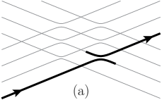
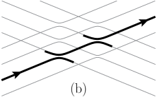
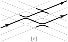
Figure 2: Transition paths from the initial states $|{\uparrow},n\rangle$, $n=0,1,2$, to the qubit state $|{\uparrow}\rangle$, i.e. those contributing to the probability $P_{{\uparrow}\to{\uparrow}}$ in the individual-crossing approximation, which is valid for weak qubit-oscillator coupling $g\ll\Omega$.

Inserting (26) into (23), we obtain the transition probability $P_{\uparrow\to\downarrow}=1-\sum_{n}p_{n}P_{{\uparrow},n\to{\uparrow}}$, where the sum can be identified as a geometric series. Evaluating this series, yields a central result, namely the Landau-Zener transition probability for finite temperature and weak qubit-oscillator coupling:

$$P_{\uparrow\to\downarrow}=f(g^{2}/v)-f(2g^{2}/v)\,\rme^{-2\pi g^{2}/v}+\big{[}f(g^{2}/v)-f(2g^{2}/v)\big{]}\rme^{2\pi g^{2}/v}\;,$$ (27)

where the temperature dependence is captured by the function

$$f(x)=\frac{1-\rme^{-\hbar\Omega/k_{{\rm B}}T}}{1-\rme^{-(\hbar\Omega/k_{{\rm B}}T+2\pi x)}}\;,$$ (28)

which for $x>0$ vanishes in the high-temperature limit, while $f(x)=1$ for zero temperature. In the latter limit, expression (27) becomes identical to equation (2). The independent-crossing approximation is valid whenever the time between the anti-crossings, $t=2v/\Omega$, exceeds the duration of an individual Landau-Zener transition, $\tau_{{\rm LZ}}\sim\sqrt{1/v}\,\max\{1,\sqrt{\Delta^{2}/v}\}$ [61]. Inserting the explicit expression (25) for $\Delta_{n}$, this condition becomes $\Omega>ng$. Thus, analytical result (27) hold only as long as oscillator states $|n\rangle$ with $n>\Omega/g$ are not thermally occupied, i.e. for $k_{{\rm B}}T<\hbar\Omega^{2}/g$. Fortunately, in the range of current experimental interest, $k_{{\rm B}}T\lesssim\hbar\Omega$ and $g<\Omega$, this condition is fulfilled. The numerical results shown in figures 3(a,b) confirm the results of the individual crossing approximation very well. Even for higher temperatures, $k_{{\rm B}}T>\hbar\Omega$, we find very good agreement, provided that the qubit-oscillator coupling $g$ is sufficiently weak, see figure 3(b). Moreover, the time evolution of the population (see figure 6, below) confirms that the dynamics indeed discerns into two individual transitions.

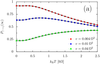
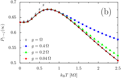
Figure 3: Spin-flip probability $P_{\uparrow\to\downarrow}$ as a function of the temperature for various sweep velocities and $g=0.04\Omega$ (a) and for various qubit-oscillator coupling strengths and $v=0.01\Omega^{2}$ (b). The symbols mark the numerical solution of the Liouville-von Neumann equation (Eq. (19) for $\gamma=0$), while the solid lines refer to the individual-crossing result (27). The dashed lines are a guide to the eye.

The temperature dependence of the spin-flip probability $P_{\uparrow\to\downarrow}$ shown in figure 3 possesses an intriguing non-monotonic behaviour: For low temperatures, $k_{{\rm B}}T\lesssim 0.2\hbar\Omega$, the probability is almost temperature independent. With an increasing temperature, $P_{\uparrow\to\downarrow}$ first becomes larger, while it eventually converges to zero in the high-temperature limit. The temperature for which the the spin-flip probability assumes a maximum is essentially independent of the qubit-oscillator coupling $g$ and increases with the sweep velocity.

This behaviour can be understood in the individual-crossing scenario sketched in figure 2. For very low temperatures, initially only the state $|{\uparrow},0\rangle$ is significantly populated and, thus, only the path sketched in figure 2(a) is relevant. For a temperature $T\approx\hbar\Omega/k_{{\rm B}}$, also the initial state $|{\uparrow},1\rangle$ becomes relevant. For this initial state, reaching the final state $|{\uparrow}\rangle$ requires two non-adiabatic transitions (see figure 2(b)) which enhances the probability to end up in state $|{\downarrow}\rangle$. With further increasing higher temperature, states $|{\uparrow},n\rangle$ with $n\geq 2$ start to play a role. In the individual-crossing picture, each of these states can evolve into four possible finale states, two of which with spin up and two with spin down (see figure 2(c)). Consequently, the probability of reaching the spin state $|{\downarrow}\rangle$ is no longer enhanced. The relevance of oscillator states with $n\geq 2$ also qualitatively explains the fact that $P_{\uparrow\to\downarrow}$ vanishes for high temperatures: In the adiabatic limit $v\ll g^{2}$, the state $|{\uparrow},n\rangle$ evolves via the state $|{\downarrow},n-1\rangle$ into the final state $|{\uparrow},n-2\rangle$. In the opposite limit of fast sweeping, the systems essentially remains in its initial state $|n,{\uparrow}\rangle$. In both cases, the qubit will predominantly end up in state $|{\uparrow}\rangle$, which complies with our numerical results.

The non-monotonic temperature dependence is in contrast to the behaviour found for Landau-Zener transitions of a qubit that is coupled to further spins, for which a monotonic temperature dependence has been conjectured [23]. The physical reason for this difference is that the spin coupled to the qubit possesses only one excited state. Then the paths sketched in figures 2(b,c), which are responsible for the non-monotonic temperature dependence, do not exist.

4 Dissipative Landau-Zener transitions

In the previous section we have studied the consequences of thermal excitations of the initial state for the transition probability (2) in the absence of an oscillator-bath coupling, i.e. for dissipation strength $\gamma=0$. We next address the question how dissipation and decoherence modify Landau-Zener tunnelling.

4.1 The zero-temperature limit

For a heat bath at zero temperature, the exact solution of the dissipative Landau-Zener problem has been derived in recent works [21, 22]. Moreover, this limit generally is rather challenging for a master equation description of quantum dissipation [46, 43]. Therefore the zero-temperature limit represents a natural test bed for our Bloch-Redfield master equation.

Let us start with a brief summary of the derivation of the exact expression for the spin-flip probability $P_{\uparrow\to\downarrow}$, as given in Ref. [22]. The central idea is to consider the cavity plus the bath as an effective bath that consists of “$\infty+1$” oscillators [32, 33, 37, 35, 38, 39, 40]. Then the qubit-oscillator coupling operator $\sigma_{x}(a+a^{{\dagger}})$ is replaced by a qubit-bath coupling of the type $\sigma_{x}\sum_{k^{\prime}}(\bar{a}^{{\dagger}}_{k^{\prime}}+\bar{a}_{k^{\prime}})$, where $(\bar{a}^{{\dagger}}_{k^{\prime}}+\bar{a}_{k^{\prime}})$ denotes the normal coordinates of the effective bath. Thus the total Hamiltonian (3) can be written in terms of the spin-boson Hamiltonian [55]

$${\mathcal{H}}_{{\rm tot}}=-\frac{{E_{\rm J}}(t)}{2}\sigma_{z}+\hbar g\sigma_{x}\sum_{k^{\prime}}\bar{c}_{k^{\prime}}(\bar{a}^{{\dagger}}_{k^{\prime}}+\bar{a}_{k^{\prime}})+\sum_{k^{\prime}}\hbar\bar{\omega}_{k^{\prime}}\bar{a}^{{\dagger}}_{k^{\prime}}\bar{a}_{k^{\prime}}.$$ (29)

Moreover, the transformation to the normal coordinates provides the effective spectral density [32, 62]

$$J_{{\rm eff}}(\omega)=g^{2}\sum_{k^{\prime}}\bar{c}_{k^{\prime}}^{2}\delta(\omega-\bar{\omega}_{k^{\prime}})=\frac{2\alpha\omega\Omega^{4}}{(\Omega^{2}-\omega^{2})^{2}+(\gamma\omega)^{2}}$$ (30)

with the effective dissipation strength

$$\alpha=\frac{4}{\pi}\frac{g^{2}}{\Omega^{3}}\gamma.$$ (31)

For the time-dependent Josephson energy ${E_{\rm J}}(t)=\hbar vt$, this model defines a dissipative Landau-Zener problem for which at $T=0$ the spin-flip probability reads [22]

$$P_{\uparrow\to\downarrow}=1-\rme^{-2\pi g^{2}\sum_{k^{\prime}}\bar{c}_{k^{\prime}}^{2}/v}.$$ (32)

Note that this formula is exact for any values of the coefficients $g$ and $\bar{c}_{k^{\prime}}$, provided that the systems starts at $t=-\infty$ in its ground state. The sum $\sum_{k^{\prime}}c_{k^{\prime}}^{2}$ can be expressed in terms of the spectral density (30), such it becomes

$$\sum_{k^{\prime}}\bar{c}_{k^{\prime}}^{2}=\frac{1}{g^{2}}\int{\rm d}\omega\,J_{{\rm eff}}(\omega)=\frac{1}{\pi}\left[\arctan\left(\frac{2\Omega^{2}-\gamma^{2}}{\gamma\sqrt{4\Omega^{2}-\gamma^{2}}}\right)+\frac{\pi}{2}\right].$$ (33)

In the limit $\gamma\to 0$, we obtain $\sum_{k^{\prime}}\bar{c}_{k^{\prime}}^{2}=1$, such that the transition probability (32) equals expression (2) which is valid in the absence of the oscillator-bath coupling. For a small but finite dissipation strength $\gamma$, $\sum_{k^{\prime}}\bar{c}_{k^{\prime}}^{2}<1$ and, thus, the spin-flip probability becomes smaller when the oscillator is damped.

We now use this exact result as a test for the master equation (10). It is worth emphasising that both problems are not fully equivalent, because the preparations are different: At zero temperature, the initial condition (22) for the master equation reads $\varrho(t=-\infty)=|{\uparrow},0\rangle\langle{\uparrow},0|$, i.e. the composed qubit-oscillator-bath system starts in the pure state $|{\uparrow},0\rangle\otimes|0,0,\ldots\rangle$, where the latter factor refers to the bath. In the analytical treatment sketched in the preceding paragraph, by contrast, the initial condition is the ground state of the total Hamiltonian (29), $|{\uparrow}\rangle\otimes|\bar{0},\bar{0},\bar{0},\ldots\rangle$. Since a finite oscillator-bath coupling induces system-bath correlations [45], the oscillator is generally entangled with the bath. Nevertheless, in the present context, the difference should be minor, because we consider a time evolution that starts at $t=-\infty$, such that the oscillator-bath setting can evolve into its ground state before Landau-Zener tunnelling occurs.

In figure 4, we compare the transition probabilities obtained with the quantum master equation (10) with the corresponding exact analytical result (32). For the system parameters used below, we find that Bloch-Redfield theory predicts even at zero temperature the exact results with an error of less than one percent. Since the quality of a Markovian quantum master equation generally improves with increasing temperature, the results presented below are rather reliable.

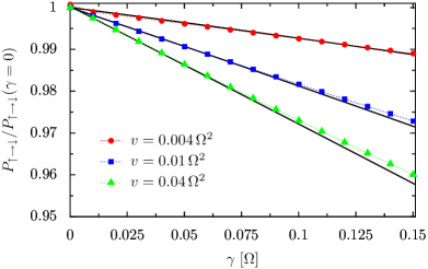
Figure 4: Comparison of the spin-flip probability $P_{\uparrow\to\downarrow}$ at $T=0$ obtained with Bloch-Redfield theory (symbols) and the exact result, Eqs. (32) and (33), as a function of the dissipation strength for qubit-oscillator coupling strength $g=0.04\Omega$ and various sweep velocities. The probability has been normalised to the corresponding value in the absence of dissipation, $P_{\uparrow\to\downarrow}(\gamma=0)$. The deviation from the exact result is always below 1%.

4.2 Thermal excitations and dissipative transitions

We next turn to the generic situation in which both thermal excitations of the initial state and dissipative transitions play a role, i.e. we consider the situation of finite temperatures and finite dissipation strength. The resulting spin-flip probabilities $P_{\uparrow\to\downarrow}$ for three different sweep velocities are shown in figure 5. For small temperatures, $k_{{\rm B}}T\lesssim 0.2\hbar\Omega$, we find that dissipation slightly reduces the spin-flip probability $P_{\uparrow\to\downarrow}$. This is consistent with the behaviour at zero temperature, discussed in section 4.1. Once the thermal energy is of the order $\hbar\Omega$, the opposite is true: dissipation supports transitions to the final ground state $|{\downarrow}\rangle$ and, thus, $P_{\uparrow\to\downarrow}$ increases. This tendency is most pronounced for the intermediate sweep velocity chosen in figure 5(b). In this regime we again find a non-monotonic temperature dependence of the transition probabilities.

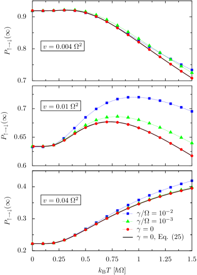
Figure 5: Damping effects on the asymptotic transition probability $P_{\uparrow\to\downarrow}$ as a function of the temperature for qubit-oscillator coupling $g=0.04\Omega$, various sweep velocities $v$ and damping strengths $\gamma$. The symbols depict numerical results obtained with the quantum master equation (19), while the solid lines mark the results from the independent-crossing approximation (27) for $\gamma=0$.

In order to reveal the role of dissipative decays, we focus on the population dynamics for an intermediate temperature $k_{{\rm B}}T\approx 0.5\hbar\Omega$, where the transition probabilities are already significantly influenced by thermal excitations; cf. figure 5. Nevertheless, the temperature is still sufficiently low, such that only the oscillator states $|0\rangle$ and $|1\rangle$ are relevant. Figure 6 shows the time evolution of the population of the states $|{\uparrow},0\rangle$ and $|{\uparrow},1\rangle$. Obviously, the populations change considerably at the avoided crossings of the qubit-oscillator spectrum, so that the dynamics discerns into three stages.

For $t<-\Omega/v$, the system remains in the canonical state. When at time $t=-\Omega/v$ the anti-crossing between the states $|{\uparrow},1\rangle$ and $|{\downarrow},0\rangle$ is reached, the population of the former state drops due to an adiabatic transition to the latter. As a consequence, the oscillator is no longer at thermal equilibrium and, consequently, we observe thermal excitations from $|{\uparrow},0\rangle$ to $|{\uparrow},1\rangle$. When at time $t=\Omega/v$, the second set of anti-crossings is reached (see figure 2(a,b)), both states undergo an individual Landau-Zener transition after which the populations converge in an oscillatory manner towards their final value. At the final stage, the oscillator populations thermalize, while those of the qubit remains practically unchanged. The latter sounds counter-intuitive because the physical system is dissipative. Nevertheless this has a physical explanation: The qubit experiences an effective heat bath with a spectral density sharply peaked at the oscillator frequency $\Omega$. Thus for large times, $t\gg\Omega/v$, the spectral density at the qubit splitting $\hbar vt$ vanishes and, consequently, the qubit is effectively decoupled from the bath.

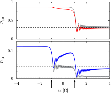
Figure 6: Population dynamics of the states $|{\uparrow},0\rangle$ (a) and $|{\uparrow},1\rangle$ (b) during the Landau-Zener sweep. Dissipation strength and temperature are $\gamma=10^{-2}\Omega$ and $k_{{\rm B}}T=0.5\hbar\Omega$, respectively. The gray lines are the corresponding results in the zero-friction limit $\gamma=0$, for which the probabilities converge to the values indicated by the dashed lines. The arrows mark the positions of the avoided crossings in the qubit oscillator spectrum; cf. figure 1.

The population dynamics provides evidence that for weak dissipation and narrowly avoided crossings, the dynamics consists of individual Landau-Zener transitions, while dissipation takes place mainly in-between the transitions. This behaviour resembles the one occurring in nanomagnets [63, 64].

5 Conclusions

We have investigated the influence of finite temperature, decoherence, and dissipation on Landau-Zener transitions of a two-level system (qubit) that is coupled via a harmonic oscillator to a heat bath. In particular, we have focussed on a recent solid-state realization of this model, namely the so-called circuit QED for which Landau-Zener sweeps can be performed by switching the effective Josephson energy of the Cooper pair box. The adiabatic spectrum of this system consists of a sequence of exact and avoided crossings, where for strong qubit-oscillator coupling, the latter may even overlap. Therefore, the resulting quantum dynamics is more complex than in the “standard” two-level Landau-Zener problem. Moreover, this qubit-oscillator-bath model is equivalent to coupling the qubit to a bath with peaked spectral density.

Dissipation has been modelled by coupling the oscillator to an Ohmic environment which we integrated out within a Bloch-Redfield approach. We solved the resulting master equation numerically after a transformation to Wigner representation followed by a decomposition into proper basis functions. The comparison with results for the exactly solvable zero-temperature limit, demonstrated that our approach provides reliable results, even though this limit is known to be rather challenging for a Markovian master equation.

For vanishing dissipation strength, the temperature enters only via initial thermal excitations of the oscillator. Most interestingly, we found for this case that the spin-flip probability exhibits a non-monotonic temperature dependence. For a sufficiently small qubit-oscillator coupling, this can be understood within the approximation of individual Landau-Zener crossings. This picture reveals the special role played by the first excited oscillator state. As compared to any other state, this state is more likely to induce a spin-flip. At intermediate temperatures, the first excited oscillator state possesses a relatively high influence, which leads to the observed non-monotonic behaviour. When dissipative decays become relevant as well, transitions to the final (adiabatic) ground state of the qubit become more likely. Nevertheless, in some small regions of parameter space, we find the opposite, namely that the probability to find the qubit in the excited state is slightly enhanced. This is at first sight counter-intuitive, but can be understood from the fact that the qubit effectively experiences a bath with a peaked spectral density. Therefore, dissipative qubit transitions can occur only during the short lapses of time in which the adiabatic energy splitting of the qubit is of the order of the oscillator frequency. With an increasing oscillator-bath coupling, the peak in the spectral density becomes broader and, thus, the more intuitive tendency towards the final ground state starts to dominate.

Finally, our results provide evidence that the recently derived zero-temperature results hold true also for finite temperatures, provided that the thermal energy does not exceed a value of roughly 20 percent of the oscillator’s energy quantum. This means that experimental quantum state preparation schemes that rely on Landau-Zener transitions in the zero-temperature limit, are feasible already when the oscillator is initially in its ground state, while the low-frequency modes of the bath may nevertheless be thermally excited.

Appendix A Derivation of the quantum master equation

In this Appendix we outline the derivation of the master equation (10) starting from the general Bloch-Redfield expression (5).

A.1 Heisenberg coupling operator

The essential step is the solution of the Heisenberg equation of motion for the scaled position operator $Q=a+a^{{\dagger}}$ of the oscillator, which will rely on approximations. In doing so, we even address a slightly more general qubit Hamiltonian outside the charge degeneracy point, i.e. we also consider the charging energy $\frac{1}{2}{E_{\rm C}}\sigma_{x}$, such that the Rabi Hamiltonian (1) becomes

$$\mathcal{H}_{\rm s}=-\frac{{E_{\rm J}}}{2}\sigma_{z}-\frac{{E_{\rm C}}}{2}\sigma_{x}+\hbar\Omega a^{{\dagger}}a+\hbar g\sigma_{x}(a^{{\dagger}}+a).$$ (34)

For convenience, we write this Hamiltonian in the eigenbasis of the qubit:

$$\mathcal{H}_{\rm s}=-\frac{\hbar\Delta}{2}\bar{\sigma}_{z}-\hbar\Omega a^{{\dagger}}a+\hbar g(\cos\theta\bar{\sigma}_{z}-\sin\theta\bar{\sigma}_{x})(a^{{\dagger}}+a),$$ (35)

where

$$\hbar\Delta=\sqrt{{E_{\rm J}}^{2}+{E_{\rm C}}^{2}},\qquad\theta=\arctan\frac{{E_{\rm J}}}{{E_{\rm C}}}$$ (36)

denote the energy splitting and the coupling angle, respectively, of the qubit. The corresponding Heisenberg equations become

$$\ddot{Q} = -\Omega^{2}Q-g\Omega(\cos\theta\bar{\sigma}_{z}-\sin\theta\bar{\sigma}_{x}),$$ (37)

$$\dot{\bar{\sigma}}_{z} = -2g\sin\theta\bar{\sigma}_{y}Q,$$ (38)

$$\dot{\bar{\sigma}}_{x} = (\Delta-2g\cos\theta)\bar{\sigma}_{y},$$ (39)

$$\dot{\bar{\sigma}}_{y} = -(\Delta-2g\cos\theta)\bar{\sigma}_{x}+2g\sin\theta\bar{\sigma}_{z}x,$$ (40)

which are non-linear due to the qubit-oscillator coupling and, thus, cannot be solved directly. We are only interested in the time evolution of the coordinate $Q$ of the oscillator with eigenfrequency $\Omega$. Since in typical circuit QED experiments $g\ll\Omega$, we treat the coupling as a perturbation. In the absence of the coupling, the time evolution of the qubit operators reads

$$\bar{\sigma}_{x}(t) = \bar{\sigma}_{x}\cos(\Delta t)+\bar{\sigma}_{y}\sin(\Delta t),$$ (41)

$$\bar{\sigma}_{z}(t) = \bar{\sigma}_{z}.$$ (42)

Inserting this into the equation of motion (37) for the oscillator coordinate, it becomes evident that the qubit entails on the oscillator the time-dependent force

$$F(t)=-g\Omega\Big{\{}\bar{\sigma}_{z}\cos\theta-\big{[}\bar{\sigma}_{x}\cos(\Delta t)+\bar{\sigma}_{y}\sin(\Delta t)\big{]}\sin\theta\Big{\}}.$$ (43)

To first order in $g$, the solution of equation (37) reads

$$Q(t)=a\rme^{{\rm i}\Omega t}+a^{{\dagger}}\rme^{-{\rm i}\Omega t}+\int_{0}^{t}{\rm d}t^{\prime}\,G(t-t^{\prime})F(t^{\prime}),$$ (44)

where

$$G(t)=\frac{\sin(\Omega t)}{\Omega}\theta(t)$$ (45)

denotes the retarded Green function of the classical dissipative harmonic oscillator. Evaluating the integral we finally obtain the Heisenberg operator

$$Q(t) = a\rme^{{\rm i}\Omega t}+a^{{\dagger}}\rme^{-{\rm i}\Omega t}-g{I_{\rm c}}(0,\Omega;t)\sigma_{z}\cos\theta$$ (46)

$$+g\big{[}{I_{\rm c}}(\Omega,\Delta;t)\sigma_{x}+{I_{\rm s}}(\Omega,\Delta;t)\sigma_{y}\big{]}\sin\theta,$$

with the functions

$${I_{\rm c}}(a,b;t) = \frac{a\cos(at)-a\cos(bt)}{a^{2}-b^{2}},$$ (47)

$${I_{\rm s}}(a,b;t) = \frac{b\sin(at)-a\sin(bt)}{a^{2}-b^{2}}.$$ (48)

Expression (46) allows one to explicitly evaluate the Bloch-Redfield equation (5).

A.2 Ohmic spectral density

In circuit QED, the environment of the qubit and the transmission line is formed by electric circuits and, thus, can be characterised by an effective impedance. In most cases, this impedance is dominated by an Ohmic resistor, which corresponds to the Ohmic spectral density (9) of the bath. Then the time integration in the Bloch-Redfield equation (5) can be evaluated. The antisymmetric correlation function (7) is then given by

$$\mathcal{A}(\tau)=\frac{\gamma}{2\pi\Omega}\int_{0}^{\infty}{\rm d}\tau\,\omega\sin(\omega\tau)=-\frac{\gamma}{2\Omega}\frac{{\rm d}}{{\rm d}\tau}\delta(\tau),$$ (49)

such that the last term of equation (5) becomes $({\rm i}\gamma/4\Omega)\dot{Q}$. The remaining time integrals are of the type

$$\int_{0}^{\infty}{\rm d}\tau\;\mathcal{S}(\tau)\cos(\Omega\tau) = \frac{\Omega}{2}\coth\Big{(}\frac{\hbar\Omega}{2k_{{\rm B}}T}\Big{)}$$ (50)

$$\int_{0}^{\infty}{\rm d}\tau\;\mathcal{S}(\tau)\sin(\Omega\tau) = \frac{\nu_{1}\Omega\omega_{{\rm c}}^{2}}{\omega_{{\rm c}}^{2}+\Omega^{2}}\sum_{n=-\infty}^{\infty}\frac{\Omega^{2}-\nu_{n}\omega_{{\rm c}}}{(\nu_{n}+\omega_{{\rm c}})(\nu_{n}^{2}+\Omega^{2})}\;,$$ (51)

where we introduced the Matsubara frequencies $\nu_{n}=2\pi nk_{{\rm B}}T/\hbar$. In the second integral, an ultraviolet divergence has been regularised by a Drude cutoff $\rme^{-\omega/\omega_{{\rm c}}}$ [44].

Appendix B Basis expansion

In this appendix we outline the diagonalisation of the oscillator Liouvillian in Wigner representation, $\mathcal{L}_{\rm{ho}}$, whose eigenvectors are used as a basis set for the numerical treatment. Since the operator $\mathcal{L}_{\rm{ho}}$, apart from the cross-diffusion $D_{xp}$, is of the same form as the Fokker-Planck operator of the corresponding problem for classical Brownian motion, we can make use of an idea put forward by Titulaer [60, 57] and generalise it along the lines of Ref. [50].

B.1 Diagonalisation of the oscillator Liouvillian

By solving the characteristic functions of the partial differential equation $\dot{\phi}=\mathcal{L}_{\rm{ho}}\phi$, one finds the operators

$$r_{+} = \partial_{x}+\frac{\lambda}{\Omega}\partial_{p}\,,$$ (52)

$$r_{-} = \frac{\Omega^{2}}{\lambda^{2}-\Omega^{2}}\Big{(}\langle Q^{2}\rangle_{{\rm eq}}\partial_{x}-\frac{\lambda}{\Omega}D_{pp}\partial_{p}+x-\frac{\lambda}{\Omega}p\Big{)},$$ (53)

which commute with $\partial/\partial t-\mathcal{L}_{\rm{ho}}$ and, thus, map any solution of the Liouville equation to a further solution. For notational convenience, we have introduced the eigenvalues of the classical equation of motion of the dissipative harmonic oscillator,

$$\lambda=-\frac{\gamma}{2}+{\rm i}\sqrt{\Omega^{2}-\frac{\gamma^{2}}{4}}\;,$$ (54)

and $\lambda^{*}$. It will turn out that the equilibrium expectation value of the dimensionless oscillator coordinate $Q$ becomes $\langle Q^{2}\rangle_{{\rm eq}}=D_{pp}+\gamma D_{xp}/\Omega$. Since moreover, the diffusion coefficient $D_{xp}$ appears in all results only in this combination, the introduction of $\langle Q^{2}\rangle_{{\rm eq}}$ turns out to be convenient as well; see also the discussion after equation (13). The operators (52) and (53) fulfil the commutation relations

$$[r_{-},r_{+}]=1\;,\quad[r_{-},r_{+}^{*}]=[r_{-}^{*},r_{+}]=0\;,\quad\left[\mathcal{L}_{\rm{ho}},r_{\pm}\right]=\pm\lambda r_{\pm}$$ (55)

and allow one to write the Liouvillian in the diagonal form

$$\mathcal{L}_{\rm{ho}}=\lambda r_{+}r_{-}+\lambda^{*}r_{+}^{*}r_{-}^{*}\;,$$ (56)

where the symbol ^∗ denotes complex conjugation. Formally we have reduced the eigenvalue problem for the Liouvillian to that of two uncoupled harmonic oscillators, so that the eigenvalues obviously read

$$\lambda_{nn^{\prime}}=\lambda n+\lambda^{*}n^{\prime}=-(n+n^{\prime})\frac{\gamma}{2}+{\rm i}(n-n^{\prime})\sqrt{\Omega^{2}-\frac{\gamma^{2}}{4}}\,,$$ (57)

where $n,n^{\prime}=0,1,2,\ldots$ The corresponding eigenfunctions $\phi_{nn^{\prime}}$ can be constructed by applying the raising operators $r_{+}$ and $r_{+}^{*}$ on the “ground state”. The latter is the stationary state defined by the relation $\mathcal{L}_{\rm{ho}}\phi_{00}=0$ whose solution is the Gaussian

$$\phi_{00}(x,p)=\frac{\Omega}{2\pi\sqrt{\langle Q^{2}\rangle_{{\rm eq}}\langle\dot{Q}^{2}\rangle_{{\rm eq}}}}\exp\Big{(}-\frac{\Omega^{2}p^{2}}{2\langle\dot{Q}^{2}\rangle_{{\rm eq}}}-\frac{x^{2}}{2\langle Q^{2}\rangle_{{\rm eq}}}\Big{)}.$$ (58)

Since $\mathcal{L}_{\rm{ho}}\neq\mathcal{L}_{\rm{ho}}^{{\dagger}}$, the eigenfunctions $\phi_{nn^{\prime}}$ are not mutually orthogonal, so that we need to compute the left eigenvectors $\bar{\phi}_{nn^{\prime}}$ of $\mathcal{L}_{\rm{ho}}$ as well. Repeating the calculation from above for $\mathcal{L}_{\rm{ho}}^{\dagger}$, we find the left ground state $\bar{\phi}_{00}=1$, so that we obtain the eigenfunctions

$$\phi_{nn^{\prime}} = \frac{1}{n!n^{\prime}!}(r_{+})^{n}(r_{+}^{*})^{n^{\prime}}\phi_{00}$$ (59)

$$\bar{\phi}_{nn^{\prime}} = (\bar{r}_{+})^{n}(\bar{r}_{+}^{*})^{n^{\prime}}\;1$$ (60)

which fulfil the ortho-normalisation relation

$$\int{\rm d}x{\rm d}p\,\bar{\phi}_{mm^{\prime}}\phi_{nn^{\prime}}=\delta_{nm}\delta_{n^{\prime}m^{\prime}}.$$ (61)

B.2 Expansion of the entire Liouvillian

Besides the already diagonalized oscillator Liouvillian, the total Liouvillian (19) for the qubit plus the oscillator contains also the operators

$$x = -r_{-}-r_{-}^{*}+\kappa r_{+}+\kappa^{*}r_{+}^{*},\qquad\kappa=\langle Q^{2}\rangle_{{\rm eq}}\frac{\Omega^{2}}{\lambda^{2}-\Omega^{2}},$$ (62)

$$\partial_{p} = -{\rm i}\frac{r_{+}-r_{+}^{*}}{2\sqrt{1-\gamma^{2}/4\Omega^{2}}}.$$ (63)

Then, the basis decomposition of the Wigner function,

$${\bf W}=\sum_{nn^{\prime}}{\bf C}_{n,n^{\prime}}\phi_{nn^{\prime}}\;;\qquad{\bf C}_{n,n^{\prime}}=\left(\begin{array}[]{cc}c_{n,n^{\prime}}^{{\uparrow}{\uparrow}}&c_{n,n^{\prime}}^{{\uparrow}{\downarrow}}\\ c_{n,n^{\prime}}^{{\downarrow}{\uparrow}}&c_{n,n^{\prime}}^{{\downarrow}{\downarrow}}\end{array}\right),$$ (64)

obeys the equation of motion

$$\dot{\bf C}_{n,n^{\prime}} = (n\lambda+n^{\prime}\lambda^{*}){\bf C}_{n,n^{\prime}}+{\rm i}\frac{{E_{\rm J}}}{2\hbar}[\sigma_{z},{\bf C}_{n,n^{\prime}}]-{\rm i}g[\sigma_{x},{\bf C}_{n+1,n^{\prime}}+{\bf C}_{n,n^{\prime}+1}]$$ (65)

$$+{\rm i}\frac{g}{\sqrt{1-\gamma^{2}/4\Omega^{2}}}[\sigma_{x},n^{\prime}{\bf C}_{n,n^{\prime}-1}-n{\bf C}_{n-1,n^{\prime}}]_{+}$$

$$+{\rm i}\frac{g}{\sqrt{1-\gamma^{2}/4\Omega^{2}}}[\sigma_{x},\kappa n{\bf C}_{n-1,n^{\prime}}-\kappa^{*}n^{\prime}{\bf C}_{n,n^{\prime}-1}]$$

$$-{\rm i}\frac{\gamma F_{\sigma}}{\sqrt{1-\gamma^{2}/4\Omega^{2}}}[\sigma_{x},n^{\prime}{\bf C}_{n,n^{\prime}-1}-n{\bf C}_{n-1,n^{\prime}}],$$

which is a set of $4N^{2}$ coupled linear ordinary differential equations.

B.3 Computation of expectation values

The expectation value of an operator can be performed directly in the basis of the eigenfunctions without back transformation to the operator representation of the density operator. For an observable

$${B}={S}\otimes{O}(x,p),$$ (66)

for which $S$ and ${O}$ refer to qubit and oscillator variables, respectively, the expectation value

$$\langle{B}\rangle=\tr\big{(}{B}\varrho\big{)}=\sum_{ij}{S}_{ij}\int{\rm d}x{\rm d}p\;{O}(x,p)\sum_{nn^{\prime}}c_{n,n^{\prime}}^{ij}\phi_{nn^{\prime}}(x,p)$$ (67)

can be expressed in terms of the operators (52) and (53) such that

$$\langle{B}\rangle=\sum_{ij}\sum_{nn^{\prime}}{S}_{ij}{O}_{nn^{\prime}}c_{n,n^{\prime}}^{ij}(t)\,,$$ (68)

where ${O}(x,p)$ is the corresponding operator in phase-space [56] and

$${O}_{nn^{\prime}}=\int{\rm d}x{\rm d}p\,O(x,p)\phi_{nn^{\prime}}(x,p).$$ (69)

If one is only interested in the behaviour of the qubit, i.e. for $O=1$, the expectation value becomes

$$\langle B\rangle=\langle{S}\rangle=\sum_{ij}{S}_{ij}\;c_{00}^{ij}(t).$$ (70)

This implies that any information about the qubit state is already contained in the four coefficients $c_{00}^{ij}(t)$, which represents a particular advantage in the present decomposition.

References

References

- [1] Nakamura Y, Pashkin Y A and Tsai J S 1999 Nature 398 786
- [2] Vion D, Aassime A, Cottet A, Joyez P, Pothier H, Urbina C, Esteve D and Devoret M H 2002 Science 296 886
- [3] Chiorescu I, Nakamura Y, Harmans C J P and Mooij J E 2003 Science 299 1869
- [4] Wallraff A, Schuster D I, Blais A, Frunzio L, Huang R S, Majer J, Kumar S, Girvin S M and Schoelkopf R J 2004 Nature 431 162
- [5] Blais A, Huang R S, Wallraff A, Girvin S M and Schoelkopf R J 2004 Phys. Rev. A 69 062320
- [6] Grajcar M et al. 2004 Phys. Rev. B 69 060501(R)
- [7] Sillanpää M A, Lehtinen T, Paila A, Makhlin Y, Roschier L and Hakonen P J 2005 Phys. Rev. Lett. 95 206806
- [8] Chiorescu I, Bertet P, Semba K, Nakamura Y, Harmans C J P M and Mooij J E 2004 Nature 431 159
- [9] Raimond J M, Brune M and Haroche S 2001 Rev. Mod. Phys. 73 565
- [10] Walther H, Varcoe B T H, Englert B G and Becker T 2006 Reports of Progress in Physics 69 1325
- [11] Sillanpää M, Lehtinen T, Paila A, Makhlin Y and Hakonen P 2006 Phys. Rev. Lett. 96 187002
- [12] Duty T, Johansson G, Bladh K, Gunnarsson D, Wilson C and Delsing P 2005 Phys. Rev. Lett. 95 206807
- [13] Sillanpää M A, Park J I and Simmonds R W 2007 Nature 449 438
- [14] Majer J et al. 2007 Nature 449 443
- [15] Saito K, Wubs M, Kohler S, Hänggi P and Kayanuma Y 2006 Europhys. Lett. 76 22
- [16] Wubs M, Kohler S and Hänggi P 2007 Physica E 40 187
- [17] Farhi E, Goldstone J, Gutmann S, Lapan J, Lundgren A and Preda D 2001 Science 292 472
- [18] Landau L D 1932 Phys. Z. Sowjetunion 2 46
- [19] Zener C 1932 Proc. R. Soc. London, Ser. A 137 696
- [20] Stueckelberg E C G 1932 Helv. Phys. Acta 5 369
- [21] Wubs M, Saito K, Kohler S, Hänggi P and Kayanuma Y 2006 Phys. Rev. Lett. 97 200404
- [22] Saito K, Wubs M, Kohler S, Kayanuma Y and Hänggi P 2007 Phys. Rev. B 75 214308
- [23] Wan A T S, Amin M H S and Wang S, arXiv:cond-mat/0703085, 2007
- [24] Gefen Y, Ben-Jacob E and Caldeira A O 1987 Phys. Rev. B 36 2770
- [25] Shimshoni E and Gefen Y 1991 Ann. Phys. (NY) 210 16
- [26] Ao P and Rammer J 1989 Phys. Rev. Lett. 62 3004
- [27] Ao P and Rammer J 1991 Phys. Rev. B 43 5397
- [28] Pokrovsky V L and Sun D 2007 Phys. Rev. B 76 024310
- [29] Kayanuma Y 1984 J. Phys. Soc. Jpn. 53 108
- [30] Saito K and Kayanuma Y 2002 Phys. Rev. A 65 033407
- [31] Vestgarden J I, Bergli J and Galperin Y M 2008 Phys. Rev. B 77 014514
- [32] Garg A, Onuchi J N and Ambegaokar V 1985 J. Chem. Phys. 83 4491
- [33] Ford G W, Lewis J T and O’Connell R F 1988 J. Stat. Phys. 53 439
- [34] Thorwart M, Hartmann L, Goychuk I and Hänggi P 2000 J. Mod. Opt. 47 2905
- [35] Thorwart M, Paladino E and Grifoni M 2004 Chem. Phys. 296 333
- [36] Wilhelm F K, Kleff S and von Delft J 2004 Chem. Phys. 296 345
- [37] van Kampen N G 2004 J. Stat. Phys. 115 1057
- [38] Ambegaokar V 2006 J. Stat. Phys. 125 1187
- [39] Ambegaokar V 2007 Ann. Phys. 16 319
- [40] Nesi F, Grifoni M and Paladino E 2007 New. J. Phys. 9 316
- [41] Yurke B and Denker J S 1984 Phys. Rev. A 29 1419
- [42] Caldeira A O and Leggett A L 1983 Ann. Phys. (N.Y.) 149 374
- [43] Hänggi P, Talkner P and Borkovec M 1990 Rev. Mod. Phys. 62 251
- [44] Weiss U 1998 Quantum Dissipative Systems, 2nd ed. (Singapore: World Scientific)
- [45] Hänggi P and Ingold G L 2005 Chaos 15 026105
- [46] Leggett A J, Chakravarty S, Dorsey A T, Fisher M P A, Garg A and Zwerger W 1987 Rev. Mod. Phys. 59 1
- [47] Ingold G L and Nazarov Y V 1992 in Charge tunneling in ultrasmall junctions, Vol. 294 of NATO ASI Series B (New York: Plenum Press), Chap. 2
- [48] Redfield A G 1957 IBM J. Res. Develop. 1 19
- [49] Blum K 1996 Density Matrix Theory and Applications (New York: Springer)
- [50] Kohler S, Dittrich T and Hänggi P 1997 Phys. Rev. E 55 300
- [51] Gardiner C W 1991 Quantum Noise, Vol. 56 of Springer Series in Synergetics (Berlin: Springer)
- [52] Tornberg L and Johansson G 2007 J. Low. Temp. 146 227
- [53] Irish E, Gea-Banacloche J, Martin I and Schwab K C 2005 Phys. Rev. B 72 195410
- [54] Caldeira A O and Leggett A J 1983 Physica A 121 587
- [55] Weiss U 1993 Quantum Dissipative Systems, Vol. 2 of Series in Modern Condensed Matter Physics (Singapore: World Scientific)
- [56] Hillery M, O’Connell R F, Scully M O and Wigner E P 1984 Phys. Rep. 106 121
- [57] Risken H 1989 The Fokker-Planck equation, Vol. 18 of Springer Series in Synergetics, 2nd ed. (Berlin: Springer)
- [58] Garcia-Palacios J L and Zueco D 2004 J. Phys.: A Math. Gen. 37 10735
- [59] Coffey W T, Kalmykov Y P, Titov S V and Mulligan B P 2007 EPL 77 2001
- [60] Titulaer U M 1978 Physica A 91 321
- [61] Mullen K, Ben-Jacob E, Gefen Y and Schuss Z 1989 Phys. Rev. Lett. 62 2543
- [62] Goorden M C, Thorwart M and Grifoni M 2004 Phys. Rev. Lett. 93 267005
- [63] Wernsdorfer W and Sessoli R 1999 Science 284 133
- [64] Giraud R, Wernsdorfer W, Tkachuk A M, Mailly D and Barbara B 2001 Phys. Rev. Lett. 87 057203