Stability and interactions of nanocolloids at fluid interfaces: effects of capillary waves and line tensions 

Abstract

We analyze the effective potential for nanoparticles trapped at a fluid interface within a simple model which incorporates surface and line tensions as well as a thermal average over interface fluctuations (capillary waves). For a single colloid, a reduced steepness of the potential well hindering movements out of the interface plane compared to rigid interface models is observed, and an instability of the capillary wave partition sum in case of negative line tensions is pointed out. For two colloids, averaging over the capillary waves leads to an effective Casimir–type interaction which is long–ranged, power-like in the inverse distance but whose power sensitively depends on possible restrictions of the colloid degress of freedom. A nonzero line tension leads to changes in the magnitude but not in the functional form of the effective potential asymptotics.

1 Introduction

The effective forces between rigid objects immersed in a fluctuating medium have attracted a steadily growing interest because their understanding allows one to design and tune them by choosing suitable media and boundary conditions and by varying the thermodynamic state of the medium. Possible applications range from micromechanical systems to colloidal suspensions and embedded biological macromolecules. Accordingly, these fluctuations may be the zero–temperature, long–ranged quantum fluctuations of the electromagnetic fields giving rise to the original Casimir effect [1] between flat or corrugated immersed metallic bodies [2, 3]. Other examples for fluctuation induced long–ranged effective forces between immersed objects involve media such as bulk fluids near their critical point [4, 5], membranes [6] or interfaces [7].

A quasi two–dimensional realization of a fluctuating system with long–ranged correlations is given by a liquid–liquid or liquid–vapor interface along with its capillary wave excitations, for an experimental study in real space see Ref. [8]. Consequently rigid objects such as colloids which are trapped at the interface are subject to an effective force generated by the fluctuating capillary waves. Theoretical investigations of this phenomenon have dealt with the effective interaction between pointlike [7] or rodlike [9] objects. If the particles are held fixed, and the interface is pinned at their surfaces, the capillary wave mediated interaction between the particles is a direct analogon of the original Casimir effect for a two–dimensional Gaussian scalar field with Dirichlet boundary conditions at the one–dimensional boundaries, given by the three–phase contact lines (for a general treatment on the Casimir effect in scalar fields, see Ref. [10]). However, the interface and the colloids are embedded in three–dimensional space, and therefore the colloids and the position of the three–phase contact lines may fluctuate. It has been shown in Refs. [11, 12, 13] that this situation corresponds theoretically to a Casimir problem with fluctuating boundary conditions. Depending on the type of admitted boundary fluctuations, the asymptotics of the resulting Casimir interaction varies considerably. This is an effect absent in the case of objects immersed in three–dimensional bulk systems. Moreover, the fluctuations of the colloids in direction perpendicular to the interface plane influence their stability, i.e. the activation energy to desorb them from the interface. This aspect has received little attention so far, as often rigid–interface models are employed to discuss the energetics of trapped colloids at interfaces (see, e.g., Refs. [14, 15]).

In this work, both questions, the stability of single colloids and their Casimir–like interactions in the presence of fluctuating capillary waves, are analyzed with particular attention to the effects of a nonzero line tension. The paper is structured as follows: In Sec. 2 we discuss a free energy model for the entrapment and stability of a single colloid at a fluid interface. In order to be self–contained, the predictions of the rigid interface models incorporating surface and line tensions are summarized in Subsecs. 2.1 and 2.2, whereas the effect of capillary waves is treated in Subsec. 2.3. In Sec. 3 we discuss the fluctuation–induced interaction between two trapped colloids, making use of the fluctuation Hamiltonians derived for the single colloid problem. The importance of the type of admitted boundary fluctuations on the effective interaction is highlighted with the exemplary discussion of two cases: (i) both colloids fluctuate freely and (ii) the colloids are held fixed. For both cases, line tensions modify the magnitude of the effective interaction but are shown not to lead to qualitatively new behavior.

2 Free energy model for spherical colloids trapped at interfaces

In this section, we consider the free energy of a single, spherical colloid with radius $R$ trapped at an interface between two phases I and II which is assumed to be flat in equilibrium. The height of the center of the colloid above the interface is denoted by $z$, and we look for the free energy $F$ of the colloid with $z$ fixed, i.e. $F\equiv F(z)$ describes a constrained free energy and the equilibrium free energy for the colloid follows upon minimization with respect to $z$. This constrained free energy can be viewed as an effective potential, in which the colloid fluctuates. In Subsecs. 2.1 and 2.2 we introduce the surface and line tension contributions to $F(z)$ under the assumption that the interface stays rigidly flat. In Subsec. 2.3 the effect of interface fluctuations on the constrained free energy $F(z)$ is calculated in a perturbative manner, employing the capillary wave concept.

2.1 Surface tension

Figure 1: Side view of a single colloid with radius $R$ trapped at an interface ($z=0$). The full circle shows the colloid in equilibrium, with ist center located at a height $z_{\rm eq}$ above the interface. The radius of the circular three–phase contact line is given by $r_{0,{\rm eq}}$. The dashed circle shows the colloid out of equilibrium at a center position $z$. The surface tensions phase I/phase II, colloid/phase I, and colloid/phase II are denoted by $\gamma$, $\gamma_{\rm I}$, and $\gamma_{\rm II}$, respectively. The physical contact angle $\theta$ differs from Young’s angle $\cos\theta_{0}=(\gamma_{\rm I}-\gamma_{\rm II})/\gamma$ for a non–vanishing line tension.

Let $\gamma$ denote the surface tension of the fluid interface and $\gamma_{\rm I[II]}$ denote the surface tension of the colloid surface (with area $A_{\rm I[II]}$) exposed to phase I [II] (see Fig. 1). The free energy $F(z)$, measured with respect to the configuration where the colloid is completely immersed in phase I, is given by [14]

$$F(z) = \gamma_{\rm I}\,(A_{\rm I}-4\pi R^{2})+\gamma_{\rm II}\,A_{\rm II}-\gamma\,A\;.$$ (1)

Here, $A$ is the cross section area of the colloid with the interface. Introducing the reduced quantities $\hat{z}=z/R$, $\hat{F}(\hat{z})=F(z)/(\pi\gamma R^{2})$, and Young’s angle $\theta_{0}$ via $\cos\theta_{0}=(\gamma_{\rm I}-\gamma_{\rm II})/\gamma$, the free energy becomes

$$\hat{F}(\hat{z}) = (\hat{z}+\cos\theta_{0})^{2}-(1+\cos\theta_{0})^{2}\;.$$ (2)

According to this model, the free energy (or single colloid effective potential) is harmonic with spring constant $k=F^{\prime\prime}(z_{\rm eq})=2\pi\gamma$. The equilibrium position is given by $\hat{z}_{\rm eq}=-\cos\theta_{0}$ and the depth of the harmonic well defines the activation energy $E_{\rm a}=\pi\gamma R^{2}(1-|\cos\theta_{0}|)^{2})$. Thus we see that for interfaces of simple fluids ($\gamma\sim 10^{-2}$ N/m) the activation energy becomes comparable to the thermal energy $\beta^{-1}=k_{\rm B}T$ only for nanoscopic colloids with radius $R\simeq 1$ nm. At such small scales the application of the simple, thermodynamic concept of surface tension seems doubtful. Nonetheless, recent investigation using computer simulations [16, 17] have indicated that the behavior of truly nanoscale particles can be described within a wide range of conditions by such a phenomenological thermodynamic model upon introduction of particle size dependent surface tensions and three–phase line tensions.

2.2 Line tension

The line tension was introduced by Gibbs [18, 19] to define the excess free energy associated to the line where three phases meet. The accurate experimental measurement of the line tension has been a considerable challenge. In fact, the uncertainty in the order of magnitude of the line tension has generated a considerable number of studies. The interested reader is referred to a recent review devoted to the current status of the three–phase line tension [20]. On theoretical grounds the line tension can be either positive or negative and it is expected to be a small force [19], $10^{-11}$ N. For simple fluids away from criticality, dimensional analysis gives $\tau\sim k_{\rm B}T/\sigma$ where $\sigma\sim 0.1$ nm is a typical atomic length scale. Line tensions inferred from experiments span several orders of magnitude, $10^{-12}-10^{-6}$ N [20, 21], reflecting the variety of experimental techniques (which are all indirect and where systematic errors can hardly be estimated) and the variety of materials used. More recent experimental efforts point towards line tensions with magnitudes at the lower end of the range given above (see, e.g., the discussion in Ref. [22] and references therein). It is not clear from the outset that the concept of line tension is unique, i.e. independent from notional shifts of the interfaces (which also shift the location of the contact line) that should be permitted within the molecularly diffuse interface region. This question is treated in detail in Ref. [22] which lines out a protocol how to define and relate line tensions obtained in different experimental setups.

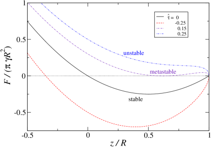
Figure 2: Plots of the reduced effective potential $\hat{F}(\hat{z})$ for 4 different values of the reduced line tension $\hat{\tau}$. With increasing $\hat{\tau}$, the configuration crosses from the stable via the metastable to the unstable regime. Young’s angle is set to $\theta_{0}=120^{o}$ which corresponds to the contact angle of $\mu$m–sized polystyrene colloids at an oil/water interface [23].

For our purposes, we may assume that a specific definition for the interface locations has been adopted with regard to which surface tensions are defined (see Fig. 1). If we associate a line tension $\tau$ with the energy of the three–phase contact line (which is a circle with radius $r_{0}=\sqrt{R^{2}-z^{2}}$), the free energy of Eq. (2) must be amended as follows:

$$\hat{F}(\hat{z}) = (\hat{z}+\cos\theta_{0})^{2}-(1+\cos\theta_{0})^{2}+2\sqrt{1-\hat{z}^{2}}\,\hat{\tau}\;.$$ (3)

Here, the reduced line tension is given by $\hat{\tau}=\tau/(\gamma R)$. The new equilibrium position of the colloid is determined by an equation of fourth order in $\hat{z}$:

$$\hat{z}_{\rm eq}\left(\frac{\hat{\tau}}{\sqrt{1-\hat{z}_{\rm eq}^{2}}}-1\right) = \cos\theta_{0}\;.$$ (4)

The spring constant $k=F^{\prime\prime}(z_{\rm eq})$ of the potential well near the minimum is also modified and becomes

$$k=2\pi\gamma(1-\hat{\tau}/\hat{r}_{0,\rm eq}^{3})$$ (5)

where $\hat{r}_{0,\rm eq}=\sqrt{1-\hat{z}_{\rm eq}^{2}}$. Note that the effective potential defined by Eq. (3) is not harmonic anymore. Positive values for the line tension lead to a shallower well, inducing metastability for the trapped colloid [15]. Large positive line tensions lead to the desorption of the colloid from the interface (see Fig. 2 for the variation of the effective potential $\hat{F}(\hat{z})$ with $\hat{\tau}$ for $\theta_{0}=120^{o}$). Thus, within this simple model, a first order transition between colloids desorbed in one of the bulk phases and adsorption to the interface is possible [15].

2.3 Capillary waves

In thermal equilibrium, the interface is not sharp but acquires a finite thickness through density fluctuations. In a coarse–grained picture, these density fluctuations correspond to fluctuations of the mean interface position $u(\mathbf{x})$ around the equilibrium position $u=0$. Here, $\mathbf{x}=(x,y)$ is a vector in the equilibrium interface plane $z=0$. For wavelengths of these interface position fluctuations which are larger than the correlation length in the bulk phases, the free energy of an interface configuration $u(\mathbf{x})$ is given by the surface energy of this configuration:

$$F_{\rm men}=\gamma\int_{S_{\rm men}}d^{2}x\left[\sqrt{1+(\nabla u)^{2}}+\frac{u^{2}}{\lambda_{c}^{2}}\right]\;.$$ (6)

Here, $S_{\rm men}$ is the interface or meniscus area projected onto the plane $z=0$ of the reference interface, i.e. it is the whole plane $z=0$ with colloids which are possibly trapped at the interface “cut out”. The free energy in Eq. (6) contains an additional term which accounts for the costs in gravitational energy associated with the meniscus fluctuations. It involves the capillary length $\lambda_{c}$ given by $\lambda_{c}=[\gamma/(|\rho_{\rm II}-\rho_{\rm I}|g)]^{1/2}$, where $g$ is the gravitational constant and $\rho_{i}$ the mass density in phase $i$. Usually, in simple fluids $\lambda_{c}$ is in the range of millimeters. Surface excitations whose free energy are described by Eq. (6) are termed capillary waves, and their effect on static and dynamic properties of liquid interfaces is a subject of lively interest [24, 25, 26, 27, 28, 29, 30].

The effective potential $F(z)$ for the colloid whose center is fixed at height $z$ above the equilibrium interface can be obtained through the partition function of the capillary waves:

$$F(z) = -k_{\rm B}T\ln\mathcal{Z}\;,$$ (7)

$$\mathcal{Z} = \mathcal{Z}_{0}^{-1}\int\mathcal{D}u\,\exp(-\beta\mathcal{H})\qquad\qquad(\beta^{-1}=k_{\rm B}T)\;.$$ (8)

Here, $\mathcal{Z}_{0}$ is a suitable normalization factor. The Hamiltonian $\mathcal{H}$ which enters the Boltzmann weight for a certain interface configuration $u(\mathbf{x})$ is the difference in free energy between the configuration $\{u(\mathbf{x}),z\}$ (describing the interface and colloid position) and the equilibrium configuration $\{u=0,z_{\rm eq}\}$ which we call the reference configuration. The equilibrium position of the colloid is determined through Eq. (4). Therefore

$$\mathcal{H}[u(\mathbf{x}),z] = (F_{\rm men}[\{u(\mathbf{x}),z\}]-F_{\rm men}[\{0,z_{\rm eq}\}])+\gamma_{\rm I}\Delta A_{\rm I}+\gamma_{\rm II}\Delta A_{\rm II}+\tau\Delta L$$ (9)

The difference in the interface areas colloid/phase I and colloid/phase II between the configuration $\{u,z\}$ and the reference configuration is given by $\Delta A_{\rm I}$ and $\Delta A_{\rm II}$, respectively, and the difference of the three–phase contact line length between these configurations is given by $\Delta L$. In general, $\mathcal{H}[u(\mathbf{x}),z]$ is a complicated functional of $u$ and $z$. In order to reduce it to a tractable expression which allows the analytical determination of the functional integral in Eq. (8), we perform a Taylor expansion in $u$ and $z$ [31]. To quadratic order, this implies that the Hamiltonian can be split into a two–dimensional “bulk” term $\mathcal{H}_{\rm cw}$ and a one–dimensional “boundary” term $\mathcal{H}_{\rm b}$:

$$\mathcal{H}[u(\mathbf{x}),z] = \left.\mathcal{H}_{\rm cw}[u(\mathbf{x})]\right|_{\mathbf{x}\in S_{\rm men,ref}}+\left.\mathcal{H}_{\rm b}[u(\mathbf{x}),z]\right|_{\mathbf{x}\in\partial S_{\rm men,ref}}\;.$$ (10)

The two–dimensional “bulk” area $S_{\rm men,ref}$ is given by the interface in the reference configuration (i.e. the plane $z=0$ with the colloid cut out), and the boundary line $\partial S_{\rm men,ref}$ is given by the three–phase contact line in the reference configuration. With these definitions $\mathcal{H}_{\rm cw}$ corresponds to the usual capillary wave Hamiltonian [32]:

$$\mathcal{H}_{\rm cw}[u(\mathbf{x})] = \frac{\gamma}{2}\int_{S_{\rm men,ref}}d^{2}x\,\left[(\nabla u)^{2}+\frac{u^{2}}{\lambda_{c}^{2}}\right]\;.$$ (11)

The boundary term $\mathcal{H}_{\rm b}$ only depends on the difference $h=z-z_{\rm eq}$ and the vertical position of the contact line $f$. The latter is expressed by its Fourier transform:

$$f(\varphi)=u(\partial S_{\rm men,ref})=\sum_{m=-\infty}^{\infty}P_{m}\,e^{{\rm i}m\varphi}\;.$$ (12)

In Eq. (12), the polar angle $\varphi$ is defined on the reference contact line circle $\partial S_{\rm men,ref}$. The Fourier coefficients $P_{m}$ are referred to as contact line multipoles below, and since the contact line height $f(\varphi)$ is real, $P_{m}=P^{*}_{-m}$ holds. With these definitions, the boundary term acquires the form

$$\mathcal{H}_{\rm b}[u(\mathbf{x}),h] = \mathcal{H}_{\rm b,1}+\mathcal{H}_{\rm b,2}\,,$$ (13)

$$\mathcal{H}_{\rm b,1} = \frac{\pi\gamma}{2}\left[2(P_{0}-h)^{2}+4\sum_{m=1}^{\infty}|P_{m}|^{2}\right]\;,$$ (14)

$$\mathcal{H}_{\rm b,2} = \frac{\pi\gamma}{2}\frac{R^{3}}{r_{0,\rm eq}^{3}}\,\hat{\tau}\left[-2\,(P_{0}-h)^{2}+4\sum_{m=1}^{\infty}\left(m^{2}-1\right)\,|P_{m}|^{2}\right]\;.$$ (15)

As before, $r_{0,\rm eq}=\sqrt{R^{2}-z_{\rm eq}^{2}}$ is the radius of the circle enclosed by the reference contact line and $\hat{\tau}=\tau/(\gamma R)$ is the reduced line tension. The detailed derivation of the two terms contributing to $\mathcal{H}_{\rm b}$ can be found in A. Note that $\mathcal{H}_{\rm b,1}$ which describes the change in colloid surface energy upon shifting the contact line is strictly positive definite, whereas $\mathcal{H}_{\rm b,2}$ is not positive definite, regardless of the sign of $\tau$.

The partition function $\mathcal{Z}$ (Eq. (8)) can be written such that the integral over contact line fluctuations $\int\mathcal{D}f$ appears explicitly:

$$\mathcal{Z}=\mathcal{Z}_{0}^{-1}\int\mathcal{D}u\,\exp\left(-\beta\mathcal{H}_{\rm cw}[u,z]\right)\;\int\mathcal{D}f\!\!\!\prod_{{\bf x}\in\partial S_{\rm men,ref}}\delta[u({\bf x})-f({\bf x})]\exp\left(-\beta\mathcal{H}_{{\rm b}}[f,h]\right)\;.\quad$$ (16)

The integration measure for the contact line fluctuations is given by $\mathcal{D}f=dP_{0}\prod_{m>0}d{\rm Re}P_{m}d{\rm Im}P_{-m}$. However, in this form the 2d-“bulk” fluctuations $u$ are not yet separated from the “boundary” fluctuations $f$. This can be achieved by splitting the field $u$ of the local interface position into a mean–field and a fluctuation part, $u=u_{\rm mf}+v$. The mean–field part solves the Euler–Lagrange equation $(-\Delta+\lambda_{c}^{-2})\,u_{\rm mf}=0$ with the boundary condition $u_{\rm mf}\,|_{\partial S_{\rm men,ref}}=f$. Consequently the fluctuation part vanishes at the contact line: $v\,|_{\partial S_{\rm men,ref}}=0$. Then the partition function $\mathcal{Z}=\mathcal{Z}_{\rm fluc}\mathcal{Z}_{\rm mf}$ factorizes into a product of a fluctuation part independent of the boundary conditions and a mean field part which depends on the fluctuating contact line $f$:

$$\mathcal{Z}_{\rm fluc} = \mathcal{Z}_{0}^{-1}\int\mathcal{D}v\,\prod_{{\bf x}\in\partial S_{\rm men,ref}}\delta(v({\bf x}))\exp\left(-\beta\mathcal{H}_{\rm cw}[v]\right)\;,$$ (17)

$$\mathcal{Z}_{\rm mf}(h) = \int\mathcal{D}f\,\exp\left\{-\frac{\beta\gamma}{2}\oint_{\partial S_{\rm men,ref}}\!\!\!\!\!\!\!\!\!\!d\ell\,f({\bf x})\,(\partial_{n}u_{\rm mf}({\bf x}))\right\}\exp\left(-\beta\mathcal{H}_{{\rm b}}[f,h]\right)\;.$$

The first exponential in $\mathcal{Z}_{\rm mf}$ stems from applying Gauss’ theorem to the energy associated with $u_{\rm mf}$. In this term $\partial_{n}u_{\rm mf}$ denotes the normal derivative of the mean–field solution towards the interior of the circle $\partial S_{\rm men,ref}$, and $d\ell$ is the infinitesimal line segment on $\partial S_{\rm men,ref}$.

Since $\mathcal{Z}_{\rm fluc}$ does not depend on the colloid position $h=z-z_{\rm eq}$, it only contributes an additive constant to the effective potential. In $\mathcal{Z}_{\rm mf}$, only the monopole fluctuations of the contact line $P_{0}$ are coupled to $h$ (see Eqs. (14) and (15)). The mean–field energy term (the first exponential in $\mathcal{Z}_{\rm mf}$, Eq. (2.3)) is diagonal in the multipole moments $P_{m}$ (see B):

$$-\frac{\beta\gamma}{2}\oint_{\partial S_{\rm men,ref}}\!\!\!\!\!\!\!\!\!\!d\ell\,f({\bf x})\,(\partial_{n}u_{\rm mf}({\bf x}))\stackrel{{\scriptstyle\lambda_{c}\gg R}}{{\simeq}}-\pi\beta\gamma\left(\frac{P_{0}^{2}}{\ln\hat{\lambda}_{c}}+2\sum_{m>0}m|P_{m}|^{2}\right)\;,$$ (18)

with the reduced capillary length given by $\hat{\lambda}_{c}=1.12\lambda_{c}/r_{0,{\rm eq}}$. Therefore only the integral over the monopole fluctuation $P_{0}$ yields a dependence on $h$ in the partition function:

$$\mathcal{Z} = \mathcal{Z}^{\prime}_{0}[v,P_{m\,(m\not=0)}]\,\int dP_{0}\exp\left\{-\pi\beta\gamma\left[\frac{P_{0}^{2}}{\ln\hat{\lambda}_{c}}+(P_{0}-h)^{2}\,\left(1-\frac{\hat{\tau}}{\hat{r}_{0,{\rm eq}}^{3}}\right)\right]\right\}$$ (19)

$$= \mathcal{Z}^{\prime}_{0}[v,P_{m\,(m\not=0)}]\,\left[\beta\gamma\left(\frac{1}{\ln\hat{\lambda}_{c}}+1-\frac{\hat{\tau}}{\hat{r}_{0,{\rm eq}}^{3}}\right)\right]^{-1/2}\;\times$$ (21)

$$\qquad\qquad\exp\left\{-\pi\beta\gamma\,h^{2}\,\frac{1-\frac{\displaystyle\hat{\tau}}{\displaystyle\hat{r}_{0,{\rm eq}}^{3}}}{1+\ln\hat{\lambda}_{c}\left(1-\frac{\displaystyle\hat{\tau}}{\displaystyle\hat{r}_{0,{\rm eq}}^{3}}\right)}\right\}$$

The $h$–independent contributions have been put into the new normalization factor $\mathcal{Z}^{\prime}_{0}$. Thus the effective potential for the colloid moving around its equilibrium position is given by

$$F(z) = -\beta^{-1}\;\ln\mathcal{Z}$$ (22)

$$= {\rm const.}+\pi\gamma\,(z-z_{\rm eq})^{2}\,\frac{1-\frac{\displaystyle\hat{\tau}}{\displaystyle\hat{r}_{0,{\rm eq}}^{3}}}{1+\ln\hat{\lambda}_{c}\left(1-\frac{\displaystyle\hat{\tau}}{\displaystyle\hat{r}_{0,{\rm eq}}^{3}}\right)}\;.$$ (23)

The spring constant $k=F^{\prime\prime}(z_{\rm eq})$ of the effective potential can be compared to the one derived for the case of a rigid interface (Eq. (5). It is seen that we recover the latter upon neglecting the term involving the capillary length $\lambda_{c}$. However, for a physical situation, the capillary length is not small and greatly diminishes the steepness of the potential well (for colloids with $R=10$ nm at an air–water interface, $\theta_{0}\simeq 90^{o}$ and negligible line tensions, $k$ is reduced by a factor of 14). In accordance with the Goldstone boson character of capillary waves, the spring constant vanishes for $\lambda_{c}\to\infty$ since the whole interface can move with no energy cost upon shifting the colloid.

In accordance with the rigid interface result (Eq. (5)), the effective potential becomes unstable for $\hat{\tau}>\hat{r}_{0,{\rm eq}}^{3}$. However, this perturbative calculation of the effective potential $F(z)$ allows no conclusion on the height of the energy barrier, which exists in the metastable regime of positive line tensions (see Fig. 2). One may speculate that the considerable reduction of the potential well steepness by capillary waves goes along with a reduction of the barrier height and would thus facilitate particle desorption.

For negative line tensions, the shape of the effective potential in Eq. (23) is hardly affected since $\ln\hat{\lambda}_{c}\gg 1$. However, an instability shows up in the partition function which is contained in the factor $\mathcal{Z}_{0}^{\prime}$. This factor contains a contribution of the form

$$\mathcal{Z}_{0}^{\prime} \propto \mathcal{D}^{\prime}f\exp\left\{-2\pi\beta\gamma\,\sum_{m>0}|P_{m}|^{2}\left[(m+1)+(m^{2}-1)\frac{\displaystyle\hat{\tau}}{\displaystyle\hat{r}_{0,{\rm eq}}^{3}}\right]\right\}$$ (24)

where the measure for the contact line fluctuations does not contain the monopoles, $\mathcal{D}^{\prime}f=\int\prod_{m>0}d{\rm Re}P_{m}d{\rm Im}P_{-m}$. Clearly, for arbitrarily small but negative $\tau$ there exists a critical multipole order $m_{c}$ above which the exponent becomes positive and thus the partition function becomes infinite. Taken at face value, for negative line tensions the interface would become unstable by forming ripples with small wavelengths near the colloid. In a physical situation, there is however a lower cutoff in the wavelength of these ripples set by the colloid surface roughness which presumably adds a positive energy penalty to higher multipole fluctuations of the contact line.

As is well–known, the capillary length $\lambda_{c}$ serves effectively as an infrared cutoff for the capillary wave spectrum. Although the capillary wave model used in this work was derived assuming gravitational damping of the capillary waves (see Eq. (6)), the dependence of all resulting expressions on $\lambda_{c}$ is not specific to that form of the capillary wave Hamiltonian [31]. Such an infrared cutoff results equally well from a finite system size (e.g. a two–phase system with trapped colloids in a container with extension $L$ or colloids trapped on a droplet with radius $R_{\rm d}$). Thus for such systems, the effective potential (Eq. (23)) is obtained by just replacing $\lambda_{c}$ by $L$ or $R_{\rm d}$. Since for smaller system sizes the influence of the line tension on $F(z)$ is more pronounced, it is conceivable to obtain a value for $\tau$ from the fluctuations in the colloid position which sample $F(z)$. As can be seen from Eq. (23), no knowledge of the surface tension $\gamma_{\rm I}$ and $\gamma_{\rm II}$ (or Young’s angle $\theta_{0}$) is required, but the modified contact angle $|\sin\theta|=\hat{r}_{0,\rm eq}$ enters. Certainly, an experimental realization appears to be difficult because of the difficulty in determining $\theta$, and one could resort to simulations in a first step which determine the colloid fluctuations with varying system size and in which $\theta$ can be determined straightforwardly.

3 Fluctuation induced forces between two colloids

The previous considerations can be extended to the case of two colloids which are trapped at the interface at distance $d$. Clearly, if both colloids are at their equilibrium position (defined by Eq. (4)) and capillary waves are neglected, the interface is flat and therefore no interface–mediated interactions are present. If, by some external force, the colloids are moved away from equilibrium, the interface will adapt to a long–ranged deformation and induce a capillary interaction energy $\propto\ln d$ between the colloids [34], the well–known cheerios effect [35]. The occurence of such a long–ranged interaction is tied to the occurence of a net force on the system “colloids + interface” [36, 31, 37].

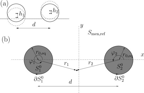
Figure 3: (a) Side view of two colloids at distance $d$ trapped at an interface, with $h_{i}$ $(i=1,2)$ denoting the relative center position of the fluctuating colloid $i$ (dashed circles) with respect to the colloid $i$ in equilibrium (full circles). (b) Top view on the equilibrium interface, spanning the $x-y$–plane. The colloids in equilibrium occupy the circular areas $S_{i}^{0}$, and their boundaries $\partial S_{i}^{0}$ are the equilibrium (or reference) three–phase contact lines.

Here, we are interested in the occurence of an interface–mediated interaction potential $V(d)$ in the force–free situation which are brought about by the fluctuating capillary waves. To that end, we can apply the partition function analysis developed in the previous section, extended to the case of two spherical “obstacles” trapped within the interface. We will focus on two scenarios:

• No external force acts on the colloids, therefore the colloids are free to fluctuate in the direction perpendicular to the interface.

• The colloids are fixed at their equilibrium position by external means. On average, there is no external force acting vertically on the colloids, although at a given instant of time some force is needed to counteract the Brownian fluctuations of the colloids. In this case, the effective potential $V(d)$ between the colloids is related to the pair correlation function $g(z_{\rm eq},z_{\rm eq},d)$ between the colloids through $\beta V(d)=-\ln g(z_{\rm eq},z_{\rm eq},d)$.

In both scenarios, the interface and in particular the three–phase contact line are free to fluctuate, subject to the energy penalty of the capillary wave and the boundary Hamiltonian lined out in the previous section. In previous work [12, 13] (neglecting line tensions) we have established that the long–range behavior of the effective potential $V(d)$ depends sensitively on the types of contact line fluctuations. For the case of a pinned contact line on the colloid and the colloids fixed at their equilibrium position, $V(d)\propto\ln\ln d$ whereas for the case (A1), $V(d)\propto d^{-8}$. In the present work, we will show (i) that for case (A2), fixed colloids but unpinned contact line, the effective potential is still long–ranged, $V(d)\propto\ln(1+\ln d)$ and (ii) that line tensions do not change the leading power in the long–range behavior of $V(d)$ but the instability for negative line tensions in the partition sum for a single colloid also occurs in the leading interaction term for case (A1).

The effective potential $V(d)$ is obtained via the partition function of the fluctuating capillary waves $\mathcal{Z}$ via

$$V(d)=-k_{\rm B}T\ln\mathcal{Z}(d)\;.$$ (25)

The partition function $\mathcal{Z}\propto\int\mathcal{D}u\,\exp(-\beta\mathcal{H})$ contains a Hamiltonian which as before contains a 2d-“bulk” term and a sum of boundary terms for each of the two colloids:

$$\mathcal{H}[u(\mathbf{x}),z] = \left.\mathcal{H}_{\rm cw}[u(\mathbf{x})]\right|_{\mathbf{x}\in S_{\rm men,ref}}+\sum_{i=1}^{2}\left.\mathcal{H}^{i}_{\rm b}[u(\mathbf{x}),z]\right|_{\mathbf{x}\in\partial S^{0}_{i}}\;.$$ (26)

The functional form of $\mathcal{H}_{\rm cw}$ and the $\mathcal{H}^{i}_{\rm b}$ is given by Eqs. (11) and (13)–(15), respectively, with due generalization of contact line multipoles for each colloid $i$, $P_{m}\to P_{im}$, and of colloid height differences $h\to h_{i}=z_{i}-z_{\rm eq}$. In the equilibrium (reference) configuration, colloid $i$ intersects the interface plane in the circular area $S^{0}_{i}$, thus the three–phase contact lines in the reference configuration are given by $\partial S^{0}_{i}$ ($i=1,2$). Thus the 2d-“bulk” area over which the capillary waves fluctuate is given by $S_{\rm men,ref}=\mathbb{R}^{2}\setminus\bigcup_{i=1}^{2}S^{0}_{i}$ (see also Fig. 3 for the geometric definitions). Via the integration domain $S_{\rm men,ref}$ of $\mathcal{H}_{\rm cw}$, the total Hamiltonian and hence the partition function $\mathcal{Z}(d)$ of the system depends on the distance $d$ of the colloid centers.

As before, the fluctuations over the contact lines $f_{i}=\sum_{m}\exp({\rm i}m\varphi_{i})P_{im}$ are incorporated into the partition function via $\delta$–function constraints:

$$\mathcal{Z}(d) = \mathcal{Z}_{0}^{-1}\int\mathcal{D}u\,\exp\left(-\beta\mathcal{H}_{\rm cw}[u,d]\right)\;\times$$

$$\prod_{\rm i=1}^{2}\int\mathcal{D}f_{i}\prod_{{\bf x}_{i}\in\partial S^{0}_{i}}\delta[u({\bf x}_{i})-f_{i}({\bf x}_{i})]\exp\left(-\beta\mathcal{H}^{i}_{{\rm b}}[f_{i},h_{i}]\right)\;.$$

The normalisation factor $\mathcal{Z}_{0}$ is chosen such that $\mathcal{Z}(d\to\infty)\to 1$. The difference between cases (A1) and (A2) defined above shows up in the definition of the measure for the contact line fluctuations:

$$\mathcal{D}f_{i} = \left\{\begin{array}[]{lr}dh_{i}\,dP_{i0}\prod_{m>0}d{\rm Re}P_{im}d{\rm Im}P_{i-m}&\quad\mbox{(A1)}\\ \\ dP_{i0}\prod_{m>0}d{\rm Re}P_{im}d{\rm Im}P_{i-m}&\quad\mbox{(A2)}\end{array}\right.\;.$$ (31)

As seen above, in the unconstrained case (A1) an additional integral over the colloid height variables is performed. Both cases can be discussed conveniently by splitting the field $u$ of the local interface position into a mean–field and a fluctuation part, $u=u_{\rm mf}+v$. The mean–field part solves the Euler–Lagrange equation $(-\Delta+\lambda_{c}^{-2})\,u_{\rm mf}=0$ with the boundary condition $u_{\rm mf}\,|_{\partial S^{0}_{i}}=f_{i}$. Consequently the fluctuation part vanishes at the contact line: $v\,|_{\partial S_{i}^{0}}=0$. Then the partition function $\mathcal{Z}=\mathcal{Z}_{\rm fluc}\mathcal{Z}_{\rm mf}$ factorises into a product of a fluctuation part independent of the boundary conditions and a mean field part which depends on the fluctuating boundary conditions $f_{i}$ of the meniscus on the colloid surfaces:

$$\mathcal{Z}_{\rm fluc} = \mathcal{Z}_{0}^{-1}\int\mathcal{D}v\,\prod_{\rm i=1}^{2}\prod_{{\bf x}_{i}\in\partial S^{0}_{i}}\delta(v({\bf x}_{i}))\exp\left(-\beta\mathcal{H}_{\rm cw}[v,d]\right)\;,$$

$$\mathcal{Z}_{\rm mf} = \prod_{\rm i=1}^{2}\int\mathcal{D}f_{i}\,\exp\left\{-\frac{\beta\gamma}{2}\sum_{i}\oint_{\partial S^{0}_{i}}d\ell_{i}f_{i}({\bf x}_{i})\,(\partial_{n}u_{\rm mf}({\bf x}_{i};d))\right\}\exp\left(-\beta\mathcal{H}^{i}_{{\rm b}}[f_{i},h_{i}]\right)\;.$$ (32)

The first exponential in $\mathcal{Z}_{\rm mf}$ stems from applying Gauss’ theorem to the energy associated with $u_{\rm mf}$. In this term $\partial_{n}u_{\rm mf}$ denotes the normal derivative of the mean–field solution towards the interior of the circle $\partial S^{0}_{i}$, and $d\ell_{i}$ is the infinitesimal line segment on $\partial S^{0}_{i}$ .

Figure 4: Pictorial representation of the separability of the total effective potential $V$ caused by the fluctuating capillary waves and the possibly fluctuating colloid into a fluctuation ($V_{\rm fluc}$) and a mean–field part ($V_{\rm men}$). The fluctuation part (second picture) is obtained by summing over all admissible capillary waves which are pinned at the colloid surface ($u=0$) and with the colloids themselves fixed. The mean–field part (third picture) is obtained by summing over the colloid height fluctuations (long arrows) and the contact line fluctuations (short arrows) equipped with a Boltzmann factor incorporating the energy of the mean–field meniscus solution whose boundary condition is set by the momentary position of the contact line.

In this form, the partition function is amenable to analytical expansions for small and large distances $d$ between the colloids. The multiplicative separation of $\mathcal{Z}$ allows to define additive contributions to the effective potential: $V=V_{\rm fluc}+V_{\rm mf}$ with $\beta V_{\rm fluc[mf]}=\ln\mathcal{Z}_{\rm fluc[mf]}$. The techniques to evaluate the fluctuation and mean–field part to the effective potential have been presented in detail in Ref. [13], and we give a summary of the main results which are necessary to discuss the influence of the line tension terms on $V(d)$.

3.1 Fluctuation part

The fluctuation part contributes equally for both cases (A1) and (A2) introduced above. The $\delta$-functions in the fluctuation part of the partition function can be removed by using their integral representation via auxiliary fields $\psi_{i}({\bf x}_{i})$ defined on the interface boundaries $\partial S^{0}_{i}$  [38]. This enables us to integrate out the field $u$ leading to

$$\mathcal{Z}_{\rm fluc}=\int\prod_{i=1}^{2}\mathcal{D}\psi_{i}\,\exp\left\{-\frac{k_{\rm B}T}{2\gamma}\sum_{i,j=1}^{2}\oint_{\partial S^{0}_{i}}d\ell_{i}\oint_{\partial S^{0}_{j}}d\ell_{j}\,\psi_{i}({\bf x}_{i})\,G(|{\bf x}_{i}-{\bf x}_{j}|)\,\psi_{j}({\bf x}_{j})\right\}\;.$$ (33)

We note in passing, that the fluctuation part in the form of Eq. (33) resembles 2d screened electrostatics: it is the partition function of a system of fluctuating charge densities $\psi_{i}$ residing on the contact circles. For large $d/r_{0}$ it can be calculated by utilizing the multipole expansion

$$\psi_{i}(\varphi_{i})=\sum_{m=-\infty}^{\infty}\psi_{im}\exp({\rm i}m\varphi_{i})\;,$$ (34)

introducing the auxiliary multipole moments $\psi_{im}$ of order $m$ pertaining to colloid $i$. Using these it can be shown that in the limit $\lambda_{c}\gg d\gg R$ the fluctuation part of the effective potential $\beta V_{\rm fluc}=-\ln\mathcal{Z}_{\rm fluc}$ has the form

$$\beta V_{\rm fluc}(d) = {\rm const.}+a_{0}(d)+\sum_{n=1}^{\infty}\frac{a_{n}}{d^{2n}},$$ (35)

$$a_{0}(d) = \frac{1}{2}\ln\ln\frac{d}{r_{0,{\rm eq}}}\;,$$ (36)

where the $a_{n}$ for $n>0$ are numerical coefficients. Through the multipole analysis it is found that interaction terms $\propto\psi_{1m}\psi_{2m^{\prime}}$ contribute terms to $V_{\rm fluc}$ which are proportional to $d^{-2(m+m^{\prime})}$. The combination $\propto\psi_{10}\psi_{20}$ (fluctuating auxiliary monopoles) gives rise to the leading term $a_{0}$ in $V_{\rm fluc}$.

3.2 Mean–field part

The calculation of $\mathcal{Z}_{\rm mf}$ (Eq. (3)) requires to determine the solution of the differential equation

$$(-\Delta+\lambda_{c}^{-2})\,u_{\rm mf}=0$$ (37)

with the boundary conditions at the fluctuating contact line and at infinity, respectively:

$$\left.u_{\rm mf}({\bf x}_{i})\right|_{{\bf x}_{i}\in\partial S^{0}_{i}} = f_{i}(\varphi_{i})$$ (38)

$$\left.u_{\rm mf}({\bf x})\right|_{|{\bf x}|\to\infty} \to 0\;.$$ (39)

We write the solution as a superposition $u_{\rm mf}=u_{1}+u_{2}$ where $u_{i}=\sum_{m}K_{m}(r_{i}/\lambda_{c})A_{im}e^{{\rm i}m\varphi_{i}}$ is the general mean–field solution in $\mathbb{R}^{2}\setminus S^{0}_{i}$ (see Fig. 3 for the geometric definitions). The solution has to match to the boundary conditions at both circles $\partial S^{0}_{1}$ and $\partial S^{0}_{2}$. This can be achieved by a projection of $u_{2}$ onto the complete set of functions on $\partial S^{0}_{1}$, $\{e^{{\rm i}m\varphi_{1}}\}$, and vice versa. Equating this expansion with the contact line multipole expansion $f_{i}(\varphi_{i})=\sum_{i}P_{i}\,\exp({\rm i}m\varphi_{i})$ leads to a system of linear equations for the expansion coefficients $\{A_{im}\}$. This system can be solved analytically within a systematic $1/d$ expansion or numerically, observing rapid convergence. Owing to the linearity of Eq. (37), the mean field part of the partition function $\mathcal{Z}_{\rm mf}$ can be written in a Gaussian form:

$$\mathcal{Z}_{\rm mf}=\int\mathcal{D}f_{i}\;\exp\left(-\beta\mathcal{H}[u_{\rm mf},d]\right)\;\exp\left\{-\pi\beta\gamma\left(1-\frac{\displaystyle\hat{\tau}}{\displaystyle\hat{r}_{0,{\rm eq}}^{3}}\right)\sum_{i}(P_{i0}-h_{i})^{2}\right\},$$ (40)

where $\mathcal{H}[u_{\rm mf}]$ is a symmetric quadratic form in the vector of the contact line multipole moments ${\bf{\hat{f}}}_{i}=(\dots,P_{i-1},P_{i0},P_{i1},\dots)$:

$$\mathcal{H}[u_{\rm mf},d] = \frac{\gamma}{2}\left(\begin{array}[]{c}{\bf\hat{f}}_{1}\\ {\bf\hat{f}}_{2}\end{array}\right)^{\rm T}\left(\begin{array}[]{cc}{\bf E}_{\rm 1\,self}&{\bf E}_{\rm int}(d)\\ {\bf E}_{\rm int}(d)&{\bf E}_{\rm 2\,self}\end{array}\right)\left(\begin{array}[]{c}{\bf\hat{f}}_{1}\\ {\bf\hat{f}}_{2}\end{array}\right)\;.$$ (47)

Using this form, it can be shown that the mean–field part $V_{\rm mf}$ of the effective potential has a similar expansion to the one of the fluctuation part $V_{\rm fluc}$ (Eq. (35)) in the limit $\lambda_{c}\gg d\gg R$:

$$\beta V_{\rm mf}(d) = {\rm const.}+b_{0}(d)+\sum_{n=1}^{\infty}\frac{b_{n}}{d^{2n}}\;.$$ (48)

Also similar to the analysis of $V_{\rm fluc}$, interaction terms $\propto P_{1m}P_{2m^{\prime}}$ contribute terms to $V_{\rm mf}$ which are proportional to $d^{-2(m+m^{\prime})}$. The fluctuating contact line monopoles and the possibly (in case (A1)) fluctuating colloid heights $h_{i}$ gives rise to the leading term $b_{0}$ in $V_{\rm mf}$. The form of $b_{0}(d)$ and the values of the numerical coefficients $b_{n}$ depend on the cases (A1) and (A2) introduced above.

• Here, for the freely fluctuating colloid, the integration measure was given by $\mathcal{D}f_{i}=dh_{i}d{\bf{\hat{f}}}_{i}$. Upon change of variables $h_{i}\to h_{i}-P_{i0}$, it is seen from Eq. (40) that the $d$–dependent part of $\mathcal{Z}_{\rm mf}$ is given by $\det{\bf E}$. For the case of vanishing line tension, the properties of $\det{\bf E}$ were discussed in detail in Ref. [13]. In particular it turns out that the four leading terms in the expansion of $V_{\rm mf}$ and $V_{\rm fluc}$ cancel each other ($b_{m}=-a_{m}$ for $m=0,1,2,3$) and the total effective potential is given to leading order by

  $$\beta V(d) \approx \frac{a_{4}+b_{4}}{d^{8}}\;.$$ (49)

  This corresponds to a quadrupole–quadrupole interaction according to the power counting in terms of the multipoles of either the fluctuating auxiliary charge densities $\psi_{im}$ (for $V_{\rm fluc}$) or the fluctuating contact line $P_{im}$ (for $V_{\rm mf}$). Hence, a nonvanishing line tension does not change the leading power in $V(d)$ since the line tension contributions (via $\mathcal{H}_{b,2}$, see Eq. (15)) to $\det{\bf E}$ are nonzero only for contact line multipoles higher than dipoles. Therefore, including the line tension we find for the total effective potential

  $$\beta V(d) = {\rm const.}-\frac{1-\frac{\displaystyle 3\,\hat{\tau}}{\displaystyle\hat{r}_{0,{\rm eq}}^{3}}\,\left(2-\frac{\displaystyle 3\hat{\tau}}{\displaystyle\hat{r}_{0,{\rm eq}}^{3}}\right)}{\left(1+\frac{\displaystyle\hat{\tau}}{\displaystyle\hat{r}_{0,{\rm eq}}^{3}}\right)^{2}}\;\frac{1}{d^{8}}$$ (50)

  The dependence of the effective potential on $\tau$ is depicted in Fig. 5. For positive line tensions, $\beta V(d)$ is always asymptotically attractive, save for the value $\hat{\tau}/r_{0,{\rm eq}}^{3}=1/3$ where the coefficient of the leading $d^{-8}$ term vanishes, and the effective potential becomes even shorter ranged. For negative line tensions, we encounter a divergence of this coefficient for $\hat{\tau}/r_{0,{\rm eq}}^{3}\to-1$. This divergence is related to the instability in the one–colloid partition function at the interface already discussed following Eq. (24).

  

  Figure 5: For case (A1), the freely fluctuating colloid, the dependence of the coefficient of the leading $d^{-8}$ term ($a_{4}+b_{4}$) in the effective potential $V(d)$ on the line tension is shown. The dependence on $\tau$ enters through the reduced variable $x=\hat{\tau}/r_{0,{\rm eq}}^{3}$ where $\hat{\tau}=\tau/(\gamma R)$ and $\hat{r}_{0,{\rm eq}}=r_{0,{\rm eq}}/R$.

• This case implies fixing the colloids at their equilibrium positions $z_{\rm eq}$. Thus in the integration measure for the contact line fluctuations the integration over the colloid height $h=z-z_{\rm eq}$ is absent, $\mathcal{D}f_{i}=d{\hat{\bf f}}_{i}$. According to Eq. (40), the quadratic form ${\hat{\bf f}}^{T}{\bf E}\;{\hat{\bf f}}$ in the Gaussian integral is slightly changed by the second exponential on the right hand side of Eq. (40). In particular, this leads to a changed leading coefficient $b_{0}$ in the mean–field free energy

  $$b_{0}(d)=-\frac{1}{2}\,\ln\ln\frac{d}{r_{0,{\rm eq}}}+\frac{1}{2}\,\ln\left(1+\left[1-\frac{\displaystyle\hat{\tau}}{\displaystyle\hat{r}_{0,{\rm eq}}^{3}}\right]\ln\frac{d}{r_{0,{\rm eq}}}\right)\;.$$ (51)

  Therefore, for case (A2) the leading term in the total effective potential contains a very long–ranged leading term of the form

  $$\beta V(d) \approx {\rm const.}+\frac{1}{2}\,\ln\left(1+\left[1-\frac{\displaystyle\hat{\tau}}{\displaystyle\hat{r}_{0,{\rm eq}}^{3}}\right]\ln\frac{d}{r_{0,{\rm eq}}}\right)\;,$$ (52)

  which for $d\gg r_{0,{\rm eq}}$ slowly approaches the asymptotic form found for $V_{\rm fluc}$ (Eq. (36)). Thus for fixed colloid position in the interface their pair correlation function $g(z_{\rm eq},z_{\rm eq},d)=-\exp(-\beta V(d))\propto-\ln(d/r_{0,{\rm eq}})$ contains a long–ranged piece dominated by the fluctuating “bulk” capillary waves only. This has also been found in a study treating the colloids as point particles [7] and in an analytical study of the pair correlation function in phase–separating 2d and 3d lattice models [39], and the asymptotics of the colloid pair correlation function is the same as exhibited by the fluid pair correlation function in the interface region [40]. However, treating the finite size of the colloids correctly leads to sizeable corrections in the asymptotics of the effective pair potential (Eq. (52)) and gives a nonzero $V(d)$ in the physically relevant case (A1) (it is zero in the limit of point colloids).

4 Conclusion

In this paper, we have studied the influence of capillary waves on the stability and interactions of colloids (with radius $R$) trapped at a fluid interface with surface tension $\gamma$, with particular attention to the effects of a line tension $\tau$. Quite often, the stability of colloids at a fluid interface with respect to vertical displacements $h$ from their equilibrium position is discussed using a rigid interface model. This gives for negligible line tensions and partially wetting colloids a steep potential well with spring constant $k=2\pi\gamma$. A finite line tension changes the spring constant by a term $\propto\tau/R$ and may induce metastability for the trapped colloids for certain positive values of $\tau$. Within a perturbative model we have found that the potential well is considerably broadened by capillary waves (qualitatively, $k\to k/\ln(\lambda_{c}/R)$ where $\lambda_{c}$ is the capillary length in the interface system). This suggests also a reduction of the metastability barriers in case of positive line tensions, although calculations beyond our perturbative model (quadratic in the fluctuations) are needed for conclusive results.

Capillary waves also induce effective interactions between two colloids which are of Casimir type. For freely fluctuating colloids a power-law dependence of the effective potential $V(d)$ in the intercolloidal distance $d$ is obtained, $V\propto d^{-8}$. A finite line tension does not change this power–law dependence, save for a specific positive value of $\tau$ where the corresponding coefficient vanishes and $V(d)$ becomes even shorter–ranged, decaying at least $\propto d^{-10}$. Negative line tensions increase the amplitude of $V(d)$. For colloids fixed in the interface, the effective potential is equivalent to the potential of mean force between them and acquires a long–ranged component $V(d)\propto\ln(1+A\ln d)$ where $A$ is a line–tension dependent coefficient (see Eq. (52)). For $d\gg R$, our results contain as a special case the long–ranged potential of mean force already discussed for pointlike colloids within an fluctuating interface.

In previous work [12, 13] we have discussed the strong attractive component in the fluctuation force which occurs for small separations between the colloid. This strong attraction is independent of the surface properties and also of the line tension and can be understood from the capillary wave partition sum with stricht Dirichlet boundary conditions on the colloid surface (see Subsec. 3.1). Both short–ranged and long–ranged regimes of the effective fluctuation potential should be important for the aggregation of nanocolloids at interfaces and compete with other effective interactions such as of electrostatic origin [41, 42].

Acknowledgment: M. O. thanks the organizers of CODEF II for their invitation and the German Science Foundation for financial support through the Collaborative Research Centre SFB-TR6 “Colloids in External Fields”, project section D6-NWG.

Appendix A Derivation of the boundary Hamiltonian

In this appendix we derive the boundary term $\mathcal{H}_{\rm b}$ which describes free energy changes upon shifting the contact line (cf. the result in Eqs. (13)–(15) of Sec. 2.3). According to Eqs. (9)–(11) the boundary term is given by

$$\mathcal{H}_{\rm b}=\gamma_{\rm I}\Delta A_{\rm I}+\gamma_{\rm II}\Delta A_{\rm II}+\gamma\Delta A_{\rm proj}+\tau\Delta L$$ (53)

and contains contributions associated with the difference in the interface areas colloid/phase I and colloid/phase II between the configuration $\{u,z\}$ and the reference configuration $\{u=0,z_{\rm eq}\}$ (given by $\Delta A_{\rm I}$ and $\Delta A_{\rm II}$, respectively) and the difference of the three–phase contact line length between these configurations (given by $\Delta L$). The term $\Delta A_{\rm proj}$ describes the change in area (with respect to the reference configuration) of meniscus $u(\mathbf{r})$ projected onto the plane $z=0$.

If the three phase contact line is slowly varying without overhangs, the following geometric relation holds between its projection onto the plane $z=0$ (parametrized in polar coordinates by $r_{0}(\varphi)$) and the contact line $u_{0}=u(r_{0}(\varphi),\varphi)$ itself:

$$r_{0}(\varphi) = \left[R^{2}-[u(r_{0}(\varphi),\varphi)-z]^{2}\right]^{1/2}$$

$$= \left[r_{0,\rm eq}^{2}+2\,z_{\rm eq}\,\left[u(r_{0}(\varphi),\varphi)-h\right]-(u(r_{0}(\varphi),\varphi)-h)^{2}\right]^{1/2}\;.$$

In Eq. (A), $r_{0,\rm eq}=\sqrt{R^{2}-z_{\rm eq}^{2}}$ is the radius of the circular reference (or equilibrium) contact line, $h=z-z_{\rm eq}$ is the deviation of the colloid center from its equilibrium height and $u(r_{0}(\varphi),\varphi)$ is the actual height of the contact line parametrized in terms of the polar angle $\varphi$.

Because of $A_{\rm II}=4\pi R^{2}-A_{\rm I}$, $\Delta A_{\rm I}=-\Delta A_{\rm II}$ holds for fluctuations of the colloid surface area in contact with fluid I and II, respectively. Then, the associated changes of the free energy can be written as

$$\gamma_{\rm I}\Delta A_{\rm I}+\gamma_{\rm II}\Delta A_{\rm II} = \gamma\cos\theta_{0}\int_{0}^{2\pi}d\varphi\int_{r_{0,\rm eq}}^{r_{0}(\varphi)}dr\,\frac{r}{\sqrt{1-r^{2}/R^{2}}}$$

$$= -R\gamma\cos\theta_{0}\,\int_{0}^{2\pi}d\varphi\,\left[u(r_{0}(\varphi),\varphi)-h\right]$$

$$\simeq -\frac{\gamma R\cos\theta_{0}}{2z_{\rm eq}}\int_{0}^{2\pi}d\varphi\,\left[f-h\right]^{2}-\frac{\gamma R\cos\theta_{0}}{2z_{\rm eq}}\int_{0}^{2\pi}d\varphi\,\left[r_{0}^{2}(\varphi)-r_{0,{\rm ref}}^{2}\right]\;,$$

where we have applied Eq. (A). Following Ref. [31], in the last line we have approximated the actual height of the contact line by the meniscus height at the reference contact circle $\partial S_{\rm men,ref}$, i.e. $u(r_{0}(\varphi),\varphi)\approx u(r_{0,{\rm eq}},\varphi)\equiv f(\varphi)$. Correction terms to this approximation are at least of third order in $u$ and $f$ [31].

The free energy contribution associated with the change in projected meniscus area can be written as

$$\gamma\Delta A_{\rm proj} = \gamma\int_{0}^{2\pi}d\varphi\int_{r_{0}(\varphi)}^{r_{0,\rm eq}}dr\,r=\frac{\gamma}{2}\int_{0}^{2\pi}d\varphi\,\left[r_{0,\rm eq}^{2}-r_{0}^{2}(\varphi)\right]\;.$$ (56)

Combining Eqs. (A) and (56), applying again Eq. (A) and using relation (4) for the equilibrium position of the colloid ($R\cos\theta_{0}/z_{\rm eq}=\tau/(\gamma r_{0,\rm eq})-1$) we find

$$\gamma_{\rm I}\Delta A_{\rm I}+\gamma_{\rm II}\Delta A_{\rm II}+\gamma\Delta A_{\rm proj} = \frac{\gamma}{2}\int_{0}^{2\pi}d\varphi\,[f-h]^{2}-\frac{\tau z_{\rm eq}}{r_{0,\rm eq}}\int_{0}^{2\pi}d\varphi\,[f-h]\;.$$ (57)

The free energy contribution related to the length fluctuations of the contact line is written as

$$\tau\Delta L = \tau\int_{0}^{2\pi}d\varphi\,\left[\sqrt{r_{0}(\varphi)^{2}+[\partial_{\varphi}r_{0}(\varphi)]^{2}+[\partial_{\varphi}u(r_{0}(\varphi),\varphi)]^{2}}-r_{0,\rm eq}\right]$$ (58)

$$\simeq \frac{\tau}{2r_{0,\rm eq}}\int_{0}^{2\pi}\!\!\!\!d\varphi\,\left[-\frac{R^{2}}{r_{0,\rm eq}^{2}}\,(f-h)^{2}+2z_{\rm eq}\,(f-h)+\frac{R^{2}}{r_{0,\rm eq}^{2}}\,(\partial_{\varphi}f)^{2}\right]$$

Comparing Eqs. (57)-(58), we find that the linear terms cancel out because the equilibrium position $z_{\rm eq}$ and $r_{0,\rm eq}$ are determined by Eq. (4). Inserting the decomposition of $f(\varphi)$ from Eq. (12) and performing the integrals over $\varphi$ finally leads to the form $\mathcal{H}_{\rm b}\simeq\mathcal{H}_{\rm b,1}+\mathcal{H}_{\rm b,2}$ given in Eqs. (13)–(15) for the the total boundary Hamiltonian, where the two contributions read

$$\mathcal{H}_{\rm b,1} = \frac{\pi\gamma}{2}\left[2(P_{0}-h)^{2}+4\sum_{m\geq 1}|P_{m}|^{2}\right]\;,$$ (59)

$$\mathcal{H}_{\rm b,2} = \frac{\pi R^{2}\tau}{2r_{0,{\rm eq}}^{3}}\left[-2\,(P_{0}-h)^{2}+4\sum_{m=1}^{\infty}\left(m^{2}-1\right)\,|P_{m}|^{2}\right]\;,$$ (60)

and describe changes in colloid surface energy and in line energy, respectively, upon shifting the three phase contact line.

Appendix B Derivation of the mean–field energy term in Eq. (18)

Let $(r,\varphi)$ be polar coordinates in the equilibrium interface plane $z=0$ where $r=0$ is the center of the circle enclosed by the reference contact line. The solution to the mean–field equation $(-\Delta+\lambda_{c}^{-2})\,u_{\rm mf}=0$ with the boundary condition $u_{\rm mf}(r_{0,{\rm eq}},\varphi)=f(\varphi)=\sum_{m}P_{m}\exp({\rm i}m\varphi)$ is given by

$$u_{\rm mf}(r,\varphi)=\sum_{m=-\infty}^{\infty}P_{m}\,\exp({\rm i}m\varphi)\,\frac{K_{|m|}\left(\frac{\displaystyle r}{\displaystyle\lambda_{c}}\right)}{K_{|m|}\left(\frac{\displaystyle r_{0,{\rm eq}}}{\displaystyle\lambda_{c}}\right)}\;,$$ (61)

where $K_{m}$ is the modified Bessel function of the second kind and order $m$. For nanocolloids, $\lambda_{c}\gg R$, so that one can use the approximation

$$K_{m}(x)\approx\left\{\begin{array}[]{cr}-\ln(x/C)\qquad(C\simeq 1.12)&(m=0)\\ (2m-2)!!\,x^{-m}&(m>0)\end{array}\right.$$ (64)

which is valid for $x\ll 1$. Thus we find (with $f^{\prime}=df/dr$)

$$\int_{0}^{2\pi}d\varphi\left(-u_{\rm mf}^{\prime}(r_{0,{\rm eq}},\varphi)\,u_{\rm mf}(r_{0,{\rm eq}},\varphi)\right)\approx\frac{2\pi}{r_{0,{\rm eq}}}\left(\frac{P_{0}^{2}}{\ln(C\lambda_{c}/r_{0,{\rm eq}})}+2\sum_{m=1}^{\infty}m|P_{m}|^{2}\right)$$ (65)

which immediately leads to Eq. (18).

References

References

- [1] Bordag M, Mohideen U and Mostepanenko V M 2001 Phys. Rep. 353 1
- [2] Jaffe R L and Scardicchio A 2004 Phys. Rev. Lett.92 070402
- [3] Büscher R and Emig T 2004 Phys. Rev.A 69 062101
- [4] Krech M 1994 The Casimir Effect in Critical Systems (Singapore: World Scientific)
- [5] Hertlein C, Helden L, Gambassi A, Dietrich S and Bechinger C 2008 Nature 451 172
- [6] Kardar M and Golestanian R 1999 Rev. Mod. Phys. 71 1233
- [7] Kaidi H, Bickel T and Benhamou M 2005 EPL 69 15
- [8] Aarts D G A L , Schmidt M and Lekkerkerker H N W 2004 Science 304 847
- [9] Golestanian R, Goulian M and Kardar M 1996 Phys. Rev.E 54 6725
- [10] Emig T, Graham N, Jaffe R L and Kardar M 2008 Phys. Rev.D 77 025005
- [11] Golestanian R 2000 Phys. Rev.E 62 5242
- [12] Lehle H, Oettel M and Dietrich S 2006 EPL 75 174
- [13] Lehle H and Oettel M 2007 Phys. Rev.E 75 011602
- [14] Pieranski P 1980 Phys. Rev. Lett.45 569
- [15] Aveyard R and Clint J H 1996 J. Chem. Soc. Farad. Trans. 92 85
- [16] Bresme F and Quirke N 1999 J. Chem. Phys.110 3536
- [17] Bresme F and Quirke N 1999 Phys. Chem. Chem. Phys. 1 2149
- [18] Gibbs J W 1961 The Scientific Papers of J. Willard Gibbs vol 1 (Ox Bow Press Connecticut) p 288
- [19] Rowlinson J S and Widom B 2002 Molecular Theory of Capillarity (New York: Dover)
- [20] Amirfazli A and Neumann A W 2004 Adv. Coll. Int. Sci. 110 121
- [21] Drelich J 1996 Colloids Surf. A 116 43
- [22] Schimmele L, Napiórkowski M and Dietrich S 2007 J. Chem. Phys.127 164715
- [23] Park B J, Pantina J P, Furst E, Oettel M, Reynaert S and Vermant J 2007 Langmuir 24 1686
- [24] Mecke K and Dietrich S 1999 Phys. Rev.E 59 6766
- [25] Fradin C, Braslau A, Luzet D, Smilgies D, Alba M, Boudet N, Mecke K and Daillant J 2000 Nature 403 871
- [26] Milchev A and Binder K 2002 EPL 59 81
- [27] Mora S, Daillant J, Mecke K, Luzet D, Braslau A, Alba M and Struth B 2003 Phys. Rev. Lett.90 216101
- [28] Madsen A, Seydel T, Sprung M, Gutt C, Tolan M and Grübel G 2004 Phys. Rev. Lett.91 096104
- [29] Vink R, Horbach J and Binder K 2005 J. Chem. Phys.122 134905
- [30] Tarazona P, Checa R and Chacón E 2007 Phys. Rev. Lett.99 196101
- [31] Oettel M, Dominguez A and Dietrich S 2005 Phys. Rev.E 71 051401
- [32] Buff F P, Lovett A and Stillinger F H 1965 Phys. Rev. Lett.15 621
- [33] Kleinert H 1990 Path integrals (Singapore: World Scientific) chapter 5
- [34] Kralchevsky P A and Nagayama K 2000 Adv. Coll. Interface Sci. 85 145
- [35] Vella D and Mahadevan L 2005 Am. J. Phys. 73 817
- [36] Foret L and Würger A 2004 Phys. Rev. Lett.92 058302
- [37] Oettel M, Dominguez A and Dietrich S 2006 Langmuir 22 846
- [38] Li H and Kardar M 1991 Phys. Rev. Lett.67 3275
- [39] Abraham D B, Essler F H and Maciolek A 2007 Phys. Rev. Lett.98 170602
- [40] Wertheim M S 1976 J. Chem. Phys.65 2377
- [41] Bresme F and Oettel M 2007 J. Phys.: Condens. Matter19 413101
- [42] Oettel M and Dietrich S 2008 Langmuir 24 1425