Reentrant phase transition in a predator prey model

Abstract

We numerically investigate the six-species predator-prey game in complex networks as well as in $d$-dimensional regular hypercubic lattices with $d=1,2,\cdots,6$. The food-web topology of the six species contains two directed loops, each of which is composed of cyclically predating three species. As the mutation rate is lowered below the well-defined phase transition point, the $Z_{2}$ symmetry related with the interchange of the two loops is spontaneously broken, and it has been known that the system develops the defensive alliance in which three cyclically predating species defend each other against the invasion of other species. In the Watts-Strogatz small-world network structure characterized by the rewiring probability $\alpha$, the phase diagram shows the reentrant behavior as $\alpha$ is varied, indicating a twofold role of the shortcuts. In $d$-dimensional regular hypercubic lattices, the system also exhibits the reentrant phase transition as $d$ is increased. We identify universality class of the phase transition and discuss the proper mean-field limit of the system.

I Introduction

Recently, nonequilibrium dynamical systems as well as standard equilibrium statistical mechanical model systems have been intensively studied in the interaction structure of complex networks review . Effects of shortcuts in the Watts-Strogatz (WS) networks WS on collective dynamic behaviors have been drawn much attention, revealing the close interplay between the structural and the dynamical properties. For networks of highly heterogeneous degree distributions such as the Barabási-Albert (BA) scale-free network BA , various aspects of collective behaviors have also been studied. Lots of existing studies have been performed in the framework of the phase transition and critical behavior review , and complex network topology in many cases gives rise to the mean-field universality class. It has been agreed that the shortcuts and the hub vertices play important roles, increasing the effective dimensionality of the WS and the BA networks, respectively, yielding the critical behavior beyond upper critical dimension. In contrast, although various nonequilibrium models like game theoretic models, epidemic spread models, the voter model, and the contact process, have been actively studied in the complex network research area review , generic understanding of how the underlying network topology affects the nonequilibrium phase transition is still lacking.

In population genetics, the so-called Lotka-Volterra model has often been studied. In the point of view of statistical physics, the neglect of the spatial density fluctuation in the original Lotka-Volterra model corresponds to a mean-field approximation, which cannot be justified in general, since every living organism inevitably lives in a finite-dimensional space with a limited range of interactions. Accordingly, population genetics models allowing spatial inhomogeneity in species densities are desirable, which can be simply realized by putting predators and preys on regular lattices in two- and three-dimensions (2D and 3D). Indeed, a cyclically interacting three-species predator-prey model has been studied both experimentally and numerically in Ref. B.Kerr, to uncover how the biodiversity of the system can be maintained. Similar three-species predator-prey model has also been investigated not in a regular lattice structure but in the small-world interaction structure G.Szabo2 . More complicated predator-prey model has been suggested later G.Szabo1 ; G.Szabo3 ; B.J.Kim2 , with six or nine species interacting with each other in a given food-web structure. In these studies it has been found that a subgroup of cyclically predating species is spontaneously formed and species within the subgroup protect the member species from the attacks by other species outside of the subgroup. The spontaneous formation of such a defensive alliance is well captured by the statistical mechanical approach and the research focus has been put on the existence and the nature of the phase transition of the spontaneous formation of alliance as the mutation rate is varied.

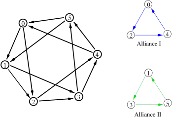
Figure 1: (Color online) Food web of the six-species predator-prey model. Each species has two predators, two preys, and two noninteracting neutral species. The two groups, called defensive alliances (alliance I and II), can be formed.

In the present work, we study the six-species predator-prey game on various spatial interaction structures, in the context of the phase transition and the critical behavior of a nonequilibrium statistical physics model in complex networks. The food web under consideration (shown in Fig. 1) has first been introduced in Ref. G.Szabo3, and later studied in Ref. B.J.Kim2, . Specifically, Szabó et al. G.Szabo3 have shown that the predator-prey game played on a 2D regular lattice exhibits a phase transition of the 2D Ising universality as the mutation rate is changed, and also identified the relevant order parameter detecting the $Z_{2}$ symmetry breaking of the defensive alliance of three cyclically predating species (see Fig. 1). In what follows, we will refer to this model as the defensive alliance process (DAP). In Ref. B.J.Kim2, the DAP has been studied on the WS network structure and the effects played by the two different types of randomness, i.e., the temporal randomness induced by the mutation, and the structural randomness introduced by the shortcuts in the WS network, have been investigated. It has also been observed that the DAP in the WS network shows a discontinuous phase transition at nonzero rewiring probability different from the continuous transition in 2D regular lattice B.J.Kim2 . We extend in this work the study in Ref. B.J.Kim2, for the WS networks and construct the complete phase diagram in the plane of the two different randomness. To investigate the role of the structural inhomogeneity, the nature of the phase transition in the regular $d$-D hypercubic lattices is also numerically studied. Since the mean-field theory developed in Ref. B.J.Kim2, does not predict a nontrivial critical point, we perform the cluster mean-field (CMF) approximation for 2D model with the hope for the better understanding as to the nature of the transition in higher dimensions.

The present paper is organized as follows: Section II presents our results of the phase diagram for the DAP on the WS networks as well as on the $d$-dimensional hypercubic lattices with $d=1,2,\cdots,6$ and discusses the reentrance transition and the nature of the phase transition. In Sec. III, the cluster mean-field theory with the cluster size 2 is developed for the 2D defensive alliance model. Finally, we summarize our results in Sec. IV.

II Defensive alliance process

We start from the description of how the DAP is implemented on general networks. The algorithm for the simulations is as follows: Initially at time $t=0$, six species are equally distributed on vertices of the given network structure, with the density $c_{s}$ of the species $s$ given by $c_{s}(t=0)=1/6$ for all species ($s=0,1,\cdots,5)$. At each time step, one vertex is chosen at random and with the probability $P$ the species at the vertex is mutated to one of its predators. Otherwise, with probability $1-P$, the species at the vertex plays the predator-prey game according to the rules depicted in Fig. 1 with one of its randomly selected neighbors, and the winner between the two occupies the loser’s vertex. If the two species are neutral, i.e., if no arrow connects the two in Fig. 1, the game will end in a draw and nothing happens. The above procedure is repeated until the system approaches the steady state.

Only for convenience, we define the parameter $\mu$ as B.J.Kim2

$$\mu=\ln(1/P),$$ (1)

which is a decreasing function of $P$. As $P$ becomes larger, the temporal randomness becomes stronger. In other words, $\mu$ resembles an inverse temperature of equilibrium systems and $1/\mu$ can be interpreted as an effective temperature.

In order to detect the alliance breaking transition we measure the order parameter $m$ (we also call it the magnetization in analogy to the ferromagnetic Ising model) defined by G.Szabo3 ; B.J.Kim2

$$m=\langle|(c_{0}+c_{2}+c_{4})-(c_{1}+c_{3}+c_{5})|\rangle,$$ (2)

where $\langle\dots\rangle$ is the time average after the steady state is achieved. In this work, a sufficiently long equilibration time (20 000 Monte-Carlo steps) is taken. As $P$ becomes larger toward unity, all species are equally probable and $m(P\rightarrow 1)=0$, while as $P$ approaches zero, the spontaneous development of defensive alliances gives us $m\approx 1$ both for the alliances I and II (see Fig. 1), indicating the possibility of a phase transition at nontrivial critical point $\mu_{c}$.

In simulating DAP, we had a numerical difficulty especially when the mutation probability $P$ is very small. In such cases, the system often spends very long time before achieving the steady state, which we try to avoid through the use of the simulated annealing technique in statistical physics by lowering $P$ slowly starting from a high value of $P$. It is also observed that if the system size is not sufficiently large, the population becomes monomorphic and all vertices are occupied by a single species before mutation acts. The rare mutation can produce a predator of the species, but the small system at the low mutation probability will again be monomorphic unless a predator of the new born predator is generated by another mutation. The results presented below are for sufficiently large systems where the polymorphic population is attained.

II.1 DAP in the WS networks

We first construct WS networks for the DAP as follows WS : (i) 1D and 2D regular lattices are first built. For 1D each vertex has connections to its four neighbors (nearest and next-nearest neighbors), whereas for 2D we assume only four nearest neighbor connections. (ii) With the rewiring probability $\alpha$ one end of each local link is moved to a randomly chosen other lattice point. Throughout this paper, we call the resulting networks as WS₁ and WS₂, respectively, in order to indicate the dimensionality $1$ and $2$ of initial regular lattices from which the WS network is built as described above. However, the subscripts $1$ and $2$ in WS₁ and WS₂ should not be interpreted as the dimensionality of the resulting small-world networks. The structure of the network is varied with $\alpha$ from a regular network ($\alpha=0$) to a fully random network ($\alpha=1$).

Except for the case of $\alpha=0$, corresponding to locally connected 1D and 2D regular lattices, the phase transition is found to be of the discontinuous nature as was already found in Ref. B.J.Kim2, : When $\mu\gtrsim\mu_{c}$, the order parameter $m$ saturates toward a finite value from below as the system size $N$ is increased, while at $\mu\lesssim\mu_{c}$, it decreases with $N$, which implies that in the thermodynamic limit of $N\rightarrow\infty$, the order parameter changes abruptly, signalling a discontinuous phase transition (see Ref. B.J.Kim2, for more detailed discussion). For examples, $m$ versus $\mu$ for the WS₁ network is shown in Fig. 2 for $\alpha=$ (a) 0.02 and (b) 0.3, with the estimation $\mu_{c}=7.4(1)$ and $\mu_{c}=6.8(1)$, respectively. We use this finite-size behavior to locate $\mu_{c}$ as above, which is then used to construct the full phase diagrams in Fig. 3.

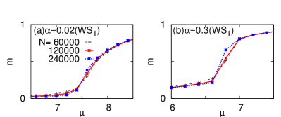
Figure 2: (Color online) The order parameter $m$ detecting the alliance breaking transition versus the mutation parameter $\mu=\ln(1/P)$ with the mutation probability $P$ is shown for the network WS₁, constructed from the 1D regular lattice via rewiring, at the rewiring probability (a) $\alpha=0.02$ and (b) $\alpha=0.3$. As $\mu$ is increased, i.e., as the mutation probability $P$ is decreased, a spontaneous formation of the defensive alliance occurs. The transition point $\mu_{c}$ is roughly estimated from the comparison of different sizes ($N=60\;000,120\;000,240\;000$): $\mu_{c}=7.4\pm 0.1$ for (a) $\alpha=0.02$ and $\mu_{c}=6.8\pm 0.1$ for (b) $\alpha=0.3$.

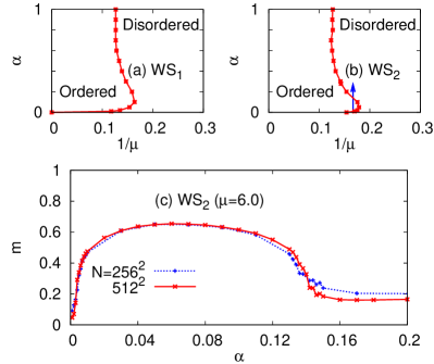
Figure 3: (Color online) Phase diagrams for the DAP in the plane of the mutation parameter $1/\mu[=1/\ln(1/P)]$ with the mutation rate $P$ and the rewiring probability $\alpha$ for (a) WS₁ and (b) WS₂ networks. As the rewiring probability $\alpha$ is changed, both (a) and (b) show reentrant phase transitions. A discontinuous phase transition is observed at any nonzero value of $\alpha$. At $\alpha=0$, WS₁ and WS₂ correspond to the regular 1D and 2D lattices. (c) $m$ versus $\alpha$ for the WS₂ networks of the sizes $N=256\times 256$ and $512\times 512$ with $\mu$ set to $6.0$, following the vertical arrow in (b). The reentrant behavior is again seen very clearly.

It is very interesting that the phase diagrams in Fig. 3 exhibit reentrant behaviors as $\alpha$ is increased. This indicates that the role of the random shortcuts is somehow twofold, facilitating the defensive alliance at small $\alpha$ and then suppressing the formation of the alliance at large $\alpha$. In detail, Fig. 3(c) displays $m$ versus the rewiring probability $\alpha$ at fixed $\mu=6.0~{}(1/\mu\approx 0.17)$ for the WS₂ network, following the vertical arrow indicated in Fig. 3(b). It is shown clearly that as $\alpha$ increases the system starts from a disordered phase with a very small $m$ and enters an ordered phase and then finally leaves back to a disordered phase. We also check the finite-size effect by comparing $m$ for two different sizes $N=256\times 256$ and $512\times 512$ in Fig. 3(c); the existence of ordered phase in the intermediate region of $\alpha$ is shown to be not a finite-size artifact. As $\alpha$ is increased from zero, more shortcuts make the system more strongly correlated in the sense that the change of the dynamic state of one vertex can affect more vertices due to the small-world effect WS . Consequently, we believe that the first increase of $m$ for small $\alpha$ can be attributed to the strengthened correlation due to more shortcuts. As $\alpha$ is increased further, the reduction of the path lengths by more shortcuts becomes less influential, and more shortcuts appear to introduce stronger spatial randomness, which eventually makes the system less ordered.

In our simulations, we also notice that the behavior of $m$ upon the change of $\mu$ is different for small $\alpha$ and large $\alpha$: When $\alpha$ is smaller than some value ($\alpha\lesssim\alpha^{*}$), the order parameter in the disordered phase $m(\mu\lesssim\mu_{c})$ approaches zero as $N$ is increased [see Fig. 2(a) for the WS₁ network at $\alpha=0.02$]. In comparison, at $\alpha\gtrsim\alpha^{*}$, $m(\mu\lesssim\mu_{c})$ remains finite as $N$ becomes larger as one can see in Fig. 2(b) for $\alpha=0.3$. It appears that $\alpha^{*}$ is close to the value of $\alpha$ at the end point of the lob structure in the phase diagram, i.e., $\alpha^{*}\approx 0.1$ for the WS₁ network.

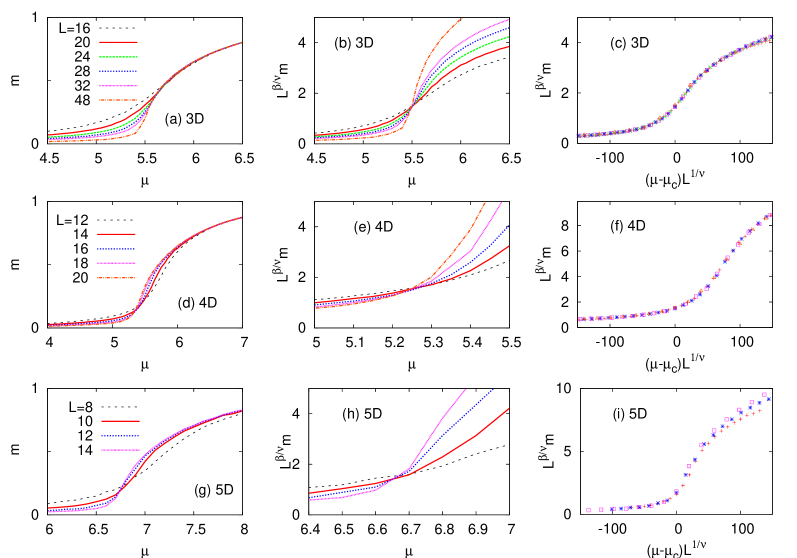
Figure 4: (Color online) Phase transitions in 3D [for (a)-(c)], 4D [for (d)-(f)], and 5D [for (g)-(i)] regular hypercubic lattices in terms of the mutation parameter $\mu$. $m$ versus $\mu$, $L^{\beta/\nu}m$ versus $\mu$, and $L^{\beta/\nu}m$ versus $(\mu-\mu_{c})L^{1/\nu}$ are shown in (a), (b), (c) for 3D, (d), (e), (f) for 4D, and (g), (h), (i) for 5D, respectively. After the determination of the critical point $\mu_{c}$ in (b), (e), (h), all data points collapse to single smooth curve by using the finite-size scaling form in Eq. (3). In 3D, $\mu_{c}\approx 5.5$, $\beta\approx 0.33$, and $\nu\approx 0.63$ are obtained in accord with the 3D Ising universality class. In 4D, on the other hand, we obtain $\mu_{c}\approx 5.25$, $\beta\approx\nu\approx 0.5$, which are the Ising mean-field exponents. In 5D, our simulation results are again consistent with the mean-field exponents $\beta\approx\nu\approx 0.5$ with $\mu_{c}\approx 6.7$.

At $\alpha=0$, WS networks do not possess any shortcuts and thus correspond to locally connected regular lattices. Observed phase transitions here at $\alpha=0$ for both WS₁ and WS₂ networks are consistent with the simple expectation that due to the underlying $Z_{2}$ symmetry of the two defensive alliances, the DAP should belong to the same universality class as the equilibrium Ising models in 1D and 2D regular lattices, i.e., no phase transition at finite $\mu$ for 1D and the phase transition with the 2D Ising critical exponents at finite $\mu_{c}$ for 2D G.Szabo3 ; B.J.Kim2 . However, the existence of discontinuous phase transition at nonzero $\alpha$ in WS₁ and WS₂ networks clearly contradicts the above simple naive expectation: It has been known that standard equilibrium models in statistical mechanics such as the Ising and the $XY$ models in the WS networks exhibit the mean-field type continuous phase transition, which has been attributed to the effective increase of the spatial dimensionality due to the shortcuts (see, e.g., Refs. Hong_Kim, ). This clearly gives a caveat that one needs to be careful in generalizing conclusions drawn for equilibrium models to nonequilibrium models.

The question we are now addressing is if the structural inhomogeneity is responsible for the discontinuous transition. Since the mean-field theory developed in Ref. B.J.Kim2, cannot predict a nontrivial critical point, the nature of the transition on the WS network cannot be understood from this theory. So it is inevitable to study regular higher-dimensional systems, especially beyond the upper critical dimensions of the Ising class. For completeness, we will study the DAP in regular 3-, 4-, and 5-dimensional hypercubic lattices in the next section, before studying 6-dimensional system in Sec. II.3.

II.2 DAP in 3-, 4-, and 5-dimensional regular lattices

The results in three-, four-, and five-dimensional regular hypercubic lattices are given in Fig. 4 for hypercubic lattices with the linear size $L$ (the total number of individual species $N=L^{d}$). We use the system size $L=16,20,24,28,32$, and $48$ for 3D, $L=12,14,16,18$, and 20 for 4D, and $L=8,10,12$ and 14 for 5D, respectively. During numerical simulations, we measure the order parameter $m$ in Eq. (2) and use the standard finite-size scaling form of the magnetization:

$$m=L^{-\beta/\nu}f\left((\mu-\mu_{c})L^{1/\nu}\right),$$ (3)

where $f(x)$ is a suitable scaling function with the scaling variable $x$, and $\beta$ and $\nu$ are critical exponents for the order parameter and the correlation length, respectively N.Goldenfeld . Figure 4 summarizes the numerical results for the phase transition in the 3D [for (a)-(c)], 4D [for (d)-(f)], and 5D [for (g)-(i)] regular hypercubic lattices. Clearly exhibited is the vanishing of the order parameter at low $\mu$ [see Fig. 4 (a), (d), and (g), in which $m$ versus $\mu$ is shown for 3D, 4D, and 5D]. The critical point $\mu_{c}$ is determined from the unique crossing point as shown in Fig. 4 (b), (e), and (h) with $L^{\beta/\nu}m$ versus $\mu$ plotted, and then we present the collapse of the numerical data into smooth curves in Fig. 4 (c), (f), and (i) for 3D, 4D, and 5D, respectively. In the above finite-size scaling analysis, the critical point $\mu_{c}$ and the critical exponents are determined: $\mu_{c}\approx 5.5$, $\beta\approx 0.33$, $\nu\approx 0.63$ in 3D, $\mu_{c}\approx 5.25$, $\beta\approx 0.5$, $\nu\approx 0.5$ in 4D, $\mu_{c}\approx 6.7$, $\beta\approx 0.5$, $\nu\approx 0.5$ in 5D. Accordingly, we conclude that the DAP belongs to the same universality class as for the equilibrium Ising model in $d$-dimensions for $d=1,2,3,4$, and $5$ N.Goldenfeld (see Table 1).

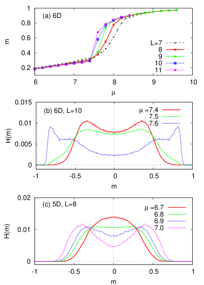
Figure 5: (Color online) (a) $m$ versus $\mu$ in 6D. From the size dependence of $m$, we roughly locate $\mu_{c}=7.4(2)$. (b) Normalized histogram $H(m)$ of the magnetization $m$ around the critical point for the system size $L=10$. The peak position suddenly changes around $\mu_{c}(L=10)\approx 7.5$, indicating the discontinuous nature of the phase transition (compare with the histogram in Ref. B.J.Kim2, for the discontinuous transition in the WS network). At large values of $\mu$, the system often exhibits asymmetric $H(m)$. Only for convenience of presentation, we symmetrized $H(m)$ to make it an even function of $m$. For comparison, we also show in (c) $H(m)$ for the 5D regular lattice of the size $L=8$. Different from (b), the peak positions in $H(m)$ changes smoothly, indicating the continuous nature of the phase transition, in accord with the mean-field universality class revealed in Fig. 4.

Table 1: Universality classes of the DAP for $d$-dimensional regular lattices, for globally-coupled structure, and for the WS network structure. The critical exponents $\beta$ and $\nu$ are included when the phase transition is of a continuous nature.

structure	$\mu_{c}$	$\beta$	$\nu$	universality class
1D regular	$\infty$	$-$	$-$	1D Ising
2D regular G.Szabo3 ; B.J.Kim2	6.5	$1/8$	$1$	2D Ising
3D regular	5.5	$0.33$	$0.63$	3D Ising
4D regular	5.25	$1/2$	$1/2$	equilibrium mean-field
5D regular	6.7	$1/2$	$1/2$	equilibrium mean-field
6D regular	7.4	$-$	$-$	discontinuous
Global coupling B.J.Kim2	$\infty$	$-$	$-$	no phase transition
WS1 and WS2	∗	$-$	$-$	discontinuous

• ^∗ $\mu_{c}$ for WS₁ and WS₂ depends on the rewiring probability $\alpha$ (see Fig. 3). When $\alpha=0$, WS₁ and WS₂ are identical to 1D and 2D regular lattices, respectively.

II.3 DAP in 6-dimensional regular lattice

We next examine the nature of the phase transition in 6D. Due to the practical limitation of the computational resources, we are limited to use the linear size $L=7,8,9,10$, and 11. Surprisingly, we find that the transition nature in 6D is very different from the simple expectation of the equilibrium mean-field type and becomes discontinuous, similarly to the WS₁ and WS₂ networks presented in Sec. II.1. In Fig. 5(a), the order parameter $m$ is shown as a function of $\mu$, exhibiting the transition around $\mu_{c}\approx 7.4$. Similarly to the WS₁ and WS₂ networks, the change of $m$ near $\mu_{c}$ becomes more abrupt as $L$ is increased, which indicates the discontinuous nature of the phase transition. In Fig. 5(b), we display the normalized histogram $H(m)$ of the order parameter $m$ [$m\equiv(c_{0}+c_{2}+c_{4})-(c_{1}+c_{2}+c_{3})$ has been used to plot $H(m)$], which clearly exhibits the signature of the discontinuous phase transition, similarly to the WS network B.J.Kim2 . As another evidence of the non-mean-field nature of the transition in 6D, we also plot $L^{\beta/\nu}$ as a function of $\mu$ in the same way as we did for 3D, 4D, and 5D in Fig. 4(b), (e), and (h)(not shown here). With the mean-filed values $\beta=\nu=1/2$, the curves do not make a unique crossing, which again supports the non-mean-field nature of the phase transition in 6D.

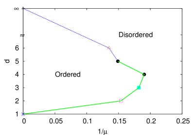
Figure 6: (Color online) Phase diagram for the DAP in $d$-dimensional regular lattices with the food web given in Fig. 1 in the plane of the mutation parameter $1/\mu$ and $d$. Different symbols denote different universality classes, and the lines are only guides to eyes. For $d=1,2,3,4$, and 5, the DAP belongs to the Ising universality class. As $d$ becomes larger, the nature of phase transition is changed to a discontinuous one. The point at $d=\infty$ is included from the result in Ref. B.J.Kim2, for the globally-coupled case.

In Fig. 6, we summarize results for the phase transitions of the DAP in $d$-dimensional hypercubic regular lattices. For $d\leq 5$, the system shares the critical behavior with the Ising model (see Table 1): No phase transition in 1D, and continuous phase transitions in 2D, 3D, 4D, and 5D with critical exponents corresponding to the Ising models in the same dimensions. Very interestingly, as the dimensionality $d$ becomes larger ($d=6$), the nature of the phase transition changes to a discontinuous one. In a sharp contrast, the equilibrium Ising model in higher dimensions than five belongs to the same mean-field universality class as in four dimension (up to logarithmic corrections), which defines the upper critical dimension of the Ising model ($d_{c}=4$). On the other hand, the DAP displays very different behavior: Although the equilibrium mean-field universality is identified in 4D and 5D, it does not lead to the conclusion that $d>5$ should exhibit the mean-field universality. From our extensive simulations of the DAP in the $d$-dimensional hypercubic regular lattices, we propose that the system has three different critical dimensions: (i) The usual lower critical dimension $d_{\rm low}=1$ below which the system is always disordered, (ii) the first upper critical dimension $d_{\rm up}^{(1)}=4$ splitting the non-mean-field transition ($d<d_{\rm up}^{(1)}$) and the mean-field transition ($d\geq d_{\rm up}^{(1)}$). Different from the equilibrium Ising model, the DAP model does not always show the mean-filed nature for dimensions higher than $d_{\rm up}^{(1)}$ and there exists (iii) the second upper critical dimension $d_{\rm up}^{(2)}=6$ beyond which the DAP shows the discontinuous phase transition. Unfortunately, we do not have any rigorous reasoning for or against the above “conjecture.”

Although the nature of the phase transition cannot be determined by the mean-field theory in Ref. B.J.Kim2, , it predicts that the critical point $1/\mu_{c}$ in $d$ dimensions should approach to 0 from above as $d\rightarrow\infty$, because the globally-coupled network is equivalent to the infinite-dimensional systems. Consequently, the vanishing value $1/\mu_{c}=0$ in both limits of $d\rightarrow\infty$ and $d=1$ makes us expect the reentrance behavior as $d$ is increased, which turns out to be true as shown in Fig. 6. This is also very different from the equilibrium Ising model in which the critical temperature monotonically increases with the dimensionality.

III Cluster Mean-Field Calculation

From our numerical observation that the discontinuous transition is not only due to the network property but it can also arise from the increased dimensionality for hypercubic regular lattices, one would expect that there will be a mean-field theory to predict the discontinuous transition. Along this direction, we apply the cluster mean-field (CMF) theory MD1999 to the two-dimensional model. In this section, the lattice point in two-dimensional square lattice is denoted by $\bm{x}$ with the decomposition $\bm{x}=n_{1}\bm{e}_{1}+n_{2}\bm{e}_{2}$, where $n_{i}$’s are integers and $\bm{e}_{i}$ are unit vector along the direction $i$. The species at site $\bm{x}$ will be denoted by $s_{\bm{x}}$.

The approximation scheme will be detailed in the Appendix and here we just sketch the calculation method. To begin with, we write down the exact evolution equation for the marginal probability (see Appendix) $P_{4}(s_{\bm{x}},s_{\bm{x}+\bm{e}_{1}},s_{\bm{x}+\bm{e}_{2}},s_{\bm{x}+\bm{e}_{1}+\bm{e}_{2}})$ from the master equation. Since each $s$ can take six different values ($s=0,1,\cdots,5$) we have to find out $6^{4}$ equations. Thanks to the spatial (rotation and inversion) and intra-alliance symmetry [$P(\{s\})=P(\{s+2\})$ with modulo 6], the number of equations is greatly reduced to 77, and the probability conservation condition reduces it to 76. To get the steady state magnetization, we numerically iterate those 76 equations until the magnetization does not change significantly. The results are summarized in Fig. 7. We then use the fitting function $m(\mu)\sim(1/\mu_{c}-1/\mu)^{\beta}$ with the mean-field critical exponent $\beta=1/2$ and estimate the critical point $\mu_{c}\simeq 6.41$, which should be compared to the Monte Carlo simulation results $\mu_{c}\simeq 6.50(4)$ in Table 1 and Ref. B.J.Kim2, . Unlike the higher-dimensional systems with $d\geq 6$, the CMF does not seem to predict the discontinuous transition although it gives us an accurate estimation of the critical point for the 2D system. However, CMF does not provide a clue to why the models in higher dimensions above 5 as well as in WS networks display the discontinuous transition. It is quite difficult to believe that the CMF with a larger cluster size than 2 can provide an explanation, because the actual transition in two dimensions is still continuous. One way might be applying the CMF to 6-dimensional systems, but it is simply too complicated to calculate.

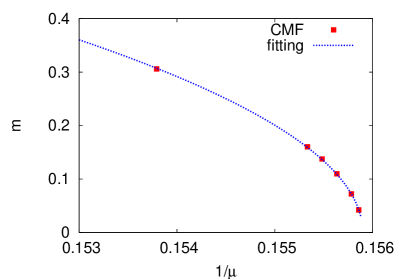
Figure 7: (Color online) Magnetization $m$ as a function of $1/\mu$ in the cluster mean-field approximation. In the fitting, $m(\mu)=A(1/\mu_{c}-1/\mu)^{1/2}$ is used with two fitting parameter $A$ and $\mu_{c}$, resulting in $\mu_{c}\simeq 6.41$.

IV Summary

We have investigated the alliance breaking phase transitions of the six-species predator prey model called the defensive alliance process (DAP) in the complex networks and also in the $d$-dimensional regular lattices. Identified nature of the phase transition is summarized in Table 1 with critical exponents included when available.

In the WS network, we have observed that the alliance breaking phase transition is of a discontinuous nature. Interesting reentrant phase transition in the WS network has been observed as the rewiring probability $\alpha$ is increased at a fixed mutation rate, implying the intricate role of the random shortcuts on the phase transition.

Hypercubic regular lattice structures in $d$ dimensions have also been used as underlying spatial interaction structure of the DAP. Observed is that the phase diagram in the plane of the dimensionality and the mutation rate again displays an interesting reentrant behavior (see Fig. 6), which is in a striking contrast to the equilibrium Ising model. For the latter model, the critical temperature is simply an increasing function of the dimensionality. We have identified the universality class for various dimensions ($d=1,2,\cdots,6$) and $d=1,2,\cdots,5$ exhibits the same critical behavior as for the equilibrium Ising model. In contrast, as $d$ is increased further, discontinuous phase transition has been observed for $d=6$. In the hope to find a theory predicting the discontinuous transition, we have applied the cluster mean-field approximation for the two-dimensional systems, but we only find the continuous transition within this scheme. Still, the reason why the higher-dimensional systems exhibit the discontinuous transition remains mystery, which can be an interesting theoretical question to be pursued further.

Appendix A Two-dimensional cluster mean-field theory

In this Appendix, the equations and symmetry of the cluster mean-field approximation with the cluster size two will be detailed. We start from deriving the exact equation for the marginal probability for the local configuration at four sites $\bm{x}$, $\bm{x}+\bm{e}_{1}$, $\bm{x}+\bm{e}_{2}$, and $\bm{x}+\bm{e}_{1}+\bm{e}_{2}$ ($\bm{x}$ is the vector designating a lattice point and $\bm{e}_{i}$’s are unit vectors along $i$-th direction).

The marginal probability $P_{4}$ is defined by

$$P_{4}(a,b,c,d)\equiv P_{4}\begin{pmatrix}a&b\\ c&d\end{pmatrix}\equiv\sum{}^{\prime}P\left(\ldots,s_{\bm{x}}=c,s_{\bm{x}+\bm{e}_{1}}=d,s_{\bm{x}+\bm{e}_{2}}=a,s_{\bm{x}+\bm{e}_{1}+\bm{e}_{2}}=b,\ldots\right),$$ (4)

where the time dependence is implicitly assumed and the primed-sum ($\sum^{\prime}$) run over the all possible configurations with four specified sites having the denoted species ($0\leq a,b,c,d\leq 5$). We always assume the modulo-6 equivalence among species indices, e.g., species 6 is equal to species 0, and so on. Due to the translational invariance, $P_{4}$ does not depend on $\bm{x}$ if initial condition does not have $\bm{x}$ dependence or if we are only interested in the stationary state. Hence we can safely omit the explicit $\bm{x}$ dependence for the function $P_{4}$.

The exact time evolution for $P_{4}$ can be written as

$$\frac{d}{dt}P_{4}\begin{pmatrix}a&b\\ c&d\end{pmatrix}=\frac{P}{2}\sum_{i=1}^{2}\left[P_{4}\begin{pmatrix}a+i&b\\ c&d\end{pmatrix}+P_{4}\begin{pmatrix}a&b+i\\ c&d\end{pmatrix}+P_{4}\begin{pmatrix}a&b\\ c+i&d\end{pmatrix}+P_{4}\begin{pmatrix}a&b\\ c&d+i\end{pmatrix}\right]-4PP_{4}\begin{pmatrix}a&b\\ c&d\end{pmatrix}$$

$$+\frac{1-P}{2}\left\{\sum_{i=1}^{2}\left[P_{5}\begin{pmatrix}a&\\ a+i&b\\ c&d\end{pmatrix}+P_{5}\begin{pmatrix}a&a+i&b\\ &c&d\end{pmatrix}+P_{5}\begin{pmatrix}&b\\ a&b+i\\ c&d\end{pmatrix}+P_{5}\begin{pmatrix}a&b+i&b\\ c&d&\end{pmatrix}+P_{5}\begin{pmatrix}a&b&\\ c&d+i&d\end{pmatrix}\right.\right.$$

$$+P_{5}\begin{pmatrix}a&b\\ c&d+i\\ &d\end{pmatrix}\left.+P_{5}\begin{pmatrix}a&b\\ c+i&d\\ c&\end{pmatrix}+P_{5}\begin{pmatrix}&a&b\\ c&c+i&d\end{pmatrix}\right]-\sum_{i=4}^{5}\Bigg{[}P_{5}\begin{pmatrix}a+i&\\ a&b\\ c&d\end{pmatrix}+P_{5}\begin{pmatrix}a+i&a&b\\ &c&d\end{pmatrix}$$

$$+P_{5}\begin{pmatrix}&b+i\\ a&b\\ c&d\end{pmatrix}+P_{5}\begin{pmatrix}a&b&b+i\\ c&d&\end{pmatrix}+P_{5}\begin{pmatrix}a&b&\\ c&d&d+i\end{pmatrix}+P_{5}\begin{pmatrix}a&b\\ c&d\\ &d+i\end{pmatrix}+P_{5}\begin{pmatrix}a&b\\ c&d\\ c+i&\end{pmatrix}$$

$$+P_{5}\begin{pmatrix}&a&b\\ c+i&c&d\end{pmatrix}\Bigg{]}+\sum_{i=1}^{2}\Bigg{[}(\delta_{ab}+\delta_{ac})P_{4}\begin{pmatrix}a+i&b\\ c&d\end{pmatrix}+(\delta_{ab}+\delta_{bd})P_{4}\begin{pmatrix}a&b+i\\ c&d\end{pmatrix}+(\delta_{ac}+\delta_{cd})P_{4}\begin{pmatrix}a&b\\ c+i&d\end{pmatrix}$$

$$+(\delta_{bd}+\delta_{cd})P_{4}\begin{pmatrix}a&b\\ c&d+i\end{pmatrix}\Bigg{]}-\left.\sum_{i=1}^{5}(1-\delta_{i3})(\delta_{a,b+i}+\delta_{a,c+i}+\delta_{b,d+i}+\delta_{c,d+i})P_{4}\begin{pmatrix}a&b\\ c&d\end{pmatrix}\right\}.$$ (5)

In Eq. (5), we also introduced $P_{5}$ which is the marginal probability of the local configuration with 5 sites, taking the form given as an argument. Due to the rotational and mirror symmetry, one can easily see that

$$P_{5}\begin{pmatrix}a&b\\ c&d\\ e&\end{pmatrix}=P_{5}\begin{pmatrix}e&c&a\\ &d&b\end{pmatrix}=P_{5}\begin{pmatrix}&d&b\\ e&c&a\end{pmatrix}.$$ (6)

Hence we do not have to deal with 8 different local configurations independently while treating $P_{5}$.

Due to the hierarchy appearing in Eq. (5) ($P_{5}$ is not reducible in terms of $P_{4}$), it is not easy to solve it exactly, which necessitates the use of the approximation scheme. To this end, we treat the correlation within squares of linear size 2 completely and neglect the correlation beyond linear length 2. To be specific, we are using the approximation scheme such that MD1999

$$P_{5}\begin{pmatrix}a&b\\ c&d\\ e&\end{pmatrix}\simeq\frac{P_{4}\begin{pmatrix}a&b\\ c&d\end{pmatrix}P_{3}\begin{pmatrix}c&d\\ e&\end{pmatrix}}{P_{2}\begin{pmatrix}c&d\end{pmatrix}},$$ (7)

where $P_{2}$ and $P_{3}$ are marginal probabilities defined similarly to $P_{4}$. The probability conservation makes it possible to find $P_{2}$ and $P_{3}$ once we know $P_{4}$ from the relations

$$P_{3}\begin{pmatrix}c&d\\ e&\end{pmatrix}=\sum_{i=0}^{5}P_{4}\begin{pmatrix}c&d\\ e&i\end{pmatrix},$$ (8)

$$P_{2}\begin{pmatrix}c&d\end{pmatrix}=\sum_{i=0}^{5}P_{3}\begin{pmatrix}c&d\\ i&\end{pmatrix}.$$ (9)

The above approximation scheme along with the symmetry consideration given in Eq. (6) lets Eq. (5) closed in the sense that the number of equations are equal to that of variables. Since it is still infeasible to solve the approximate equation analytically, we resort to the numerical solutions.

One may treat the $6^{4}=1296$ equations directly without considering the degeneracy of $P_{4}$’s. However, symmetry consideration reduces the number of equations we have to deal with considerably. Now we will show that actually we have only to treat 76 equations to get the full solution.

There are three symmetry operations which are summarized as follows:

$$P_{4}\begin{pmatrix}a&b\\ c&d\end{pmatrix}=P_{4}\begin{pmatrix}b&d\\ a&c\end{pmatrix}=P_{4}\begin{pmatrix}c&a\\ d&b\end{pmatrix},$$ (10)

$$P_{4}\begin{pmatrix}a&b\\ c&d\end{pmatrix}=P_{4}\begin{pmatrix}b&a\\ d&c\end{pmatrix}=P_{4}\begin{pmatrix}a&c\\ b&d\end{pmatrix},$$ (11)

$$P_{4}\begin{pmatrix}a&b\\ c&d\end{pmatrix}=P_{4}\begin{pmatrix}a+2&b+2\\ c+2&d+2\end{pmatrix},$$ (12)

which are rotation ($\pm 90^{\circ}$), mirror (against the diagonal axes), and intra-ally symmetric operations, respectively. To find the degeneracy due to symmetry, let us first categorize the local configurations according to the number of same species among 4 sites. There are 5 such categories which take the form $\{0,0,0,0\}$ (6), $\{0,0,0,1\}$ (120), $\{0,0,1,1\}$ (90), $\{0,0,1,2\}$ (720), and $\{0,1,2,3\}$ (360), where the species numbers in curly brackets are just for the representative purpose, the order of four elements in the curly braces are irrelevant, and the numbers in parentheses indicate the total number of local configurations of the corresponding categories whose sum should be $6^{4}$.

By considering the above symmetry operations, we reduce the number of independent variables. When $a=b=c=d$, the intra-ally symmetry reduces the independent variables from 6 to 2. When three of four species are the same such as $a=b=c\neq d$, rotational symmetry as well as the intra-ally one reduces the number of independent variables. For example, $P_{4}(a,a,a,d)=P_{4}(a,a,d,a)=P_{4}(a,d,a,a)=P_{4}(d,a,a,a)$ by rotation and $P_{4}(a,a,a,d)=P_{4}(a+2,a+2,a+2,d+2)$ by intra-ally transformations. From this consideration, one can find that there are 10 independent variables out of 120 variables. In case $a=b\neq c=d$, the symmetry consideration shows that (we omit $P_{4}$ for convenience)

$$\begin{pmatrix}a&a\\ c&c\end{pmatrix}=\begin{pmatrix}a&c\\ a&c\end{pmatrix}=\begin{pmatrix}c&c\\ a&a\end{pmatrix}=\begin{pmatrix}c&a\\ c&a\end{pmatrix},$$

$$\begin{pmatrix}a&c\\ c&a\end{pmatrix}=\begin{pmatrix}c&a\\ a&c\end{pmatrix},$$ (13)

which reduces the independent variables from 90 to 30. The intra-ally symmetry once again reduces the number from 30 to 10.

The fourth case is $a=b\neq c\neq d\neq a$. The symmetry enforces the equivalence among configurations such that

$$\begin{pmatrix}a&a\\ c&d\end{pmatrix}=\begin{pmatrix}a&d\\ a&c\end{pmatrix}=\begin{pmatrix}d&c\\ a&a\end{pmatrix}=\begin{pmatrix}c&a\\ d&a\end{pmatrix},$$

$$\begin{pmatrix}a&c\\ d&a\end{pmatrix}=\begin{pmatrix}c&a\\ a&d\end{pmatrix},$$ (14)

where exchanging $c$ with $d$, which is equivalent to the mirror transformation, also gives the equivalent configurations. Hence Eq. (14) combined with the intra-ally symmetry reduces the number from 720 to 40. The last category contains all different species. This category has $\binom{6}{4}=15$ elements. Since the rotation and the mirror symmetry operations always conserve the diagonal relations, each set has 3 different classes. Due to the intra-ally symmetry, however, only 15 configurations remain independent. To sum all independent configurations, we find that there are 77 (=2+10+10+40+15) independent variables. Due to the probability conservation, one equations becomes reducible by other variables. So the final number of independent variables is 76.

One may solve the stationary state solution by setting $\partial/\partial t=0$ in Eq. (5). For us, this turned out not to be easy, so we numerically integrate Eq. (5) starting from the fully magnetized state with intra-ally symmetry such that $P_{4}(a,b,c,d)=1/3^{n}$ with $n$ to be the number of members in alliance I among $a,b,c,d$ and found the stationary state magnetization, which is summarized in Fig. 7.

References

- (1) S.N. Dorogovtsev and A.V. Goltsev, and J.F.F. Mendes, Rev. Mod. Phys. 80, 1275 (2008); R. Albert and A.-L. Barabási, ibid. 74, 47 (2002); S.N. Dorogovtsev and J.F.F. Mendes, Adv. Phys. 51, 1079 (2002); M.E.J. Newman, SIAM Rev. 45, 167 (2003).
- (2) D.J. Watts and S.H. Strogatz, Nature (London) 393, 440 (1998).
- (3) A.-L. Barabási and R. Albert, Science 286, 509 (1999).
- (4) B. Kerr, M.A. Riley, M.W. Feldman, and B.J.M. Bohannan, Nature (London) 418, 171 (2002).
- (5) G. Szabó, A. Szolnoki, and R. Izsák, J. Phys. A: Math. Gen. 37, 2599 (2004).
- (6) G. Szabó and T. Czárán, Phys. Rev. E 63, 061904 (2001).
- (7) G. Szabó and T. Czárán, Phys. Rev. E 64, 042902 (2001).
- (8) B.J. Kim, J. Liu, J. Um, and S.-I. Lee, Phys. Rev. E 72, 041906 (2005).
- (9) H. Hong, B.J. Kim, and M.Y. Choi, Phys. Rev. E 66, 018101 (2002); K. Medvedyeva, P. Holme, P. Minnhagen, and B.J. Kim, ibid. 67, 036118 (2003); B.J. Kim, H. Hong, P. Holme, G.S. Jeon, P. Minnhangen, and M.Y. Choi, ibid. 64, 056135 (2001).
- (10) See, e.g., N. Goldenfeld, Lecture on Phase Transitions and Renormalization Group (Addison-Wesley, MA 1992).
- (11) J. Marro and R. Dickman, Nonequilibrium Phase Transitions in Lattice Models (Cambridge University Press, Cambridge, 1999).