Spatial Interference Cancellation for Multi-Antenna Mobile Ad Hoc Networks

Abstract

Interference between nodes is a critical impairment in mobile ad hoc networks (MANETs). This paper studies the role of multiple antennas in mitigating such interference. Specifically, a network is studied in which receivers apply zero-forcing beamforming to cancel the strongest interferers. Assuming a network with Poisson distributed transmitters and independent Rayleigh fading channels, the transmission capacity is derived, which gives the maximum number of successful transmissions per unit area. Mathematical tools from stochastic geometry are applied to obtain the asymptotic transmission capacity scaling and characterize the impact of inaccurate channel state information (CSI). It is shown that, if each node cancels $L$ interferers, the transmission capacity decreases as $\Theta(\epsilon^{\frac{1}{L+1}})$ as the outage probability $\epsilon$ vanishes. For fixed $\epsilon$, as $L$ grows, the transmission capacity increases as $\Theta(L^{1-\frac{2}{\alpha}})$ where $\alpha$ is the path-loss exponent. Moreover, CSI inaccuracy is shown to have no effect on the transmission capacity scaling as $\epsilon$ vanishes, provided that the CSI training sequence has an appropriate length, which we derived. Numerical results suggest that canceling merely one interferer by each node increases the transmission capacity by an order of magnitude or more, even when the CSI is imperfect.

I Introduction

In a mobile ad hoc network (MANET), the mutual interference between nodes poses a fundamental limit on the throughput of peer-to-peer communication. This paper studies mitigating the effect of interference by provisioning nodes with multiple antennas. Specifically, each receiver uses zero-forcing beamforming to cancel the interference from the strongest interferers, whereas each transmitter simply chooses a random beam. This approach requires only limited local coordination and hence is suitable for a MANET.

This paper considers a simple network consisting of Poisson distributed transmitters and independent Rayleigh fading channels. We quantify the gains in network performance in terms of the transmission capacity (TC) as a function of the system parameters, including the amount and accuracy of channel state information (CSI) at each receiver. The TC is defined in [1] as the maximum density of successful transmissions so that a typical receiver satisfies an outage probability constraint for a target signal-to-interference-and-noise ratio (SINR). In other words, TC gives the average throughput per unit area. The derived TC scaling suggests that multiple antennas can significantly improve the performance of MANETs, even with inaccurate CSI.

I-A Prior Work and Motivation

For Poisson distributed transmitters, TC was introduced in [1] for single-antenna MANETs assuming fixed transmission power and an ALOHA-like medium access control (MAC) layer. TC has also been used to study opportunistic transmissions [2], distributed scheduling [3], coverage [4], network irregularity [5], bandwidth partitioning [6], successive interference cancellation [7], and multi-antenna transmission [8] in MANETs [9]. This paper differs from [8] in that the antennas are employed for interference cancellation instead of interference averaging through diversity techniques. After the publication of preliminary results from the current investigation [10, 11], related work has been reported on the TC of multi-antenna MANETs that use spatial multiplexing and space-time block coding [12], space division multiple access [13], or optimally allocate the spatial degrees of freedom for interference cancellation and link enhancement such as spatial multiplexing [14] and array gain [15].

As discussed in [2], the TC is related to the more widely known transport capacity introduced in [16]. Transport capacity is typically studied in terms of the scaling of a network’s total throughput-distance product as a function of the network size, while TC gives the number of single-hop transmissions possible in a specific area and in terms of the actual design parameters. Furthermore, most work on the transport capacity assumes perfect scheduling and zero-outage, while we focus on a random access model with an outage requirement.

Besides spatial interference cancellation, there are several alternative approaches for mitigating interference in MANETs. For example, the interference alignment approach in [17] achieves the optimal number of degrees of freedom in a high signal-to-noise ratio (SNR) setting. This approach appears daunting in practice because it requires jointly designed precoders and perfect CSI of interference channels. In contrast, the current approach only requires each receiver to obtain CSI from nearby interferers and no coordination of transmit precoders. Another method for interference management, used in many practical MAC protocols, is to create an interferer-free area – a guard zone – around each receiving node through carrier sensing. As shown in [3], optimizing the guard-zone size leads to significant TC gain for a single-antenna MANET with respect to pure random access. The use of interference cancellation can be viewed as creating an effective guard zone without requiring that other nearby transmitters be suppressed.

Several papers have addressed other aspects of multi-antenna MANETs. For example, beamforming or directional antennas have been integrated with the MAC protocols for MANETs to achieve higher network spatial reuse or energy efficiency [18, 19, 20, 21, 22, 23, 24, 25, 26, 27]. In addition, multi-antenna techniques have been applied to enable efficient routing in MANETs [28]. Directional antennas have been studied for suppressing interference in MANETs by spatial filtering [23, 24, 25, 26, 27]. Directional antennas, however, are only suitable for environments with sparse scattering and low angular spread. In contrast, beamforming is applicable for both sparse and rich scattering, and is hence adopted in this paper as well as in [19, 20, 21] for spatial interference cancellation. Most prior work focuses on designing MAC protocols and rely on simulations for throughput evaluation [29, 18, 19, 20, 21, 22, 23, 24, 25, 26, 27]. In [30, 31], the use of directional antennas is shown to increase the linear scaling factor of network transport capacity, which, however, is too coarse for quantifying the network throughput. In view of prior work, there still lacks theoretic characterization of the relationship between the TC of MANETs and spatial interference cancellation.

I-B Contributions and Organization

Our main contributions are summarized as follows.

1. Assuming Poisson distributed transmitters and spatially independently and identically distributed (i.i.d.) Rayleigh fading channels, bounds on the probability of signal-to-interference ratio (SIR) outage are derived with either perfect or imperfect CSI. These bounds are found to be reasonably tight and lead to bounds on TC.

2. Let $L$ denote the number of canceled interferers per receiver. Irrespective of whether the CSI is perfect, as the outage probability $\epsilon$ vanishes, the asymptotic TC is shown to vanish as $\epsilon^{\frac{1}{L+1}}$, which decays slower for larger $L$.

3. For fixed $\epsilon$, as $L\rightarrow\infty$, the TC is shown to increase as $L^{1-\frac{2}{\alpha}}$ where $\alpha$ is the path-loss exponent. Hence spatial interference cancellation is more effective for larger $\alpha$. If instead of canceling interference, the antennas are used to maximize the array gain, the TC scales as $L^{\frac{2}{\alpha}}$ as shown in [8].

4. The required training sequence length for CSI estimation is derived for constraining the increase in outage probability and loss in data rate caused by imperfect interference cancellation. Finally, the required training sequence length is obtained for the optimal TC scaling and shown to be proportional to $\log\frac{1}{\epsilon}$.

Simulation results show that canceling a few (two to four) interferers per node is sufficient for harvesting most of the available TC gain. A capacity gain of more than an order of magnitude can be achieved by canceling only one interferer at each node, even with imperfect CSI. Moreover, a moderate length of the CSI training sequence is observed to be sufficient.

The remainder of this paper is organized as follows. Section II describes the network and wireless channel models. The SIR outage probability and TC are analyzed for perfect and imperfect CSI in Sections III and IV, respectively. Numerical results are presented in Section V.

II Mathematical Models and Metrics

II-A Network Model

The locations of potential transmitting nodes in a MANET are modeled as a 2-D Poisson point process with density $\lambda_{o}$ following the common approach in the literature (see e.g., [32]). Time is slotted and in each time-slot potential transmitting nodes follow a random access protocol, namely that they transmit independently with a fixed probability $P_{t}$. Let $T$ denote the coordinate of a transmitting node. Given the random access protocol, the set $\acute{\Phi}=\{T\}$ is also a homogeneous Poisson point process but with smaller density $\lambda=P_{t}\lambda_{o}$ [33]. Each transmitting node is associated with a receiving node located at a unit distance. Relaxing the assumption that a transmitter and a receiver are separated by a fixed distance affects the TC scaling only by a multiplicative factor (see e.g, [2]).

Consider a typical receiving node located at the origin, denoted as $R_{0}$, and let $T_{0}$ be the corresponding transmitter. This constraint on $R_{0}$ and $T_{0}$ does not compromise generality since the transmitting node process is translation invariant. Furthermore, according to Slivnyak’s theorem [34, Section 4.4], the remaining transmitting nodes, namely $\Phi=\acute{\Phi}\backslash\{T_{0}\}$, remain a homogeneous Poisson point process with the same density $\lambda$.

The MANET is assumed to be interference limited and thus noise is neglected for simplicity. Consequently, the reliability of data packets received by $R_{0}$ is determined by the SIR. Moreover, we assume that each data link has a single stream, and communications between nodes are perfectly synchronized at symbol boundaries. All transmitting nodes are assumed to use unit transmission power.

II-B Channel Model

Let every node be equipped with $N$ antennas, so that the link between each transmitter and receiver can be modeled as an $N\times N$ multiple-input-multiple-output (MIMO) channel. We assume narrowband channels with frequency-flat block fading. Moreover, each MIMO channel consists of path-loss and small-scale fading components. Specifically, the channel from $T\in\acute{\Phi}$ to $R_{0}$ is $r_{T}^{-\alpha/2}{\mathbf{G}}_{T}$, where $\alpha>2$ is the path-loss exponent, and ${\mathbf{G}}_{T}$ is an $N\times N$ matrix of i.i.d. unit circularly symmetric complex Gaussian elements (we subsequently denote the distribution as $\mathcal{CN}(0,1)$). Beamforming is applied at each transmitter and receiver, where ${\mathbf{f}}_{0}$, ${\mathbf{f}}_{T}$ and ${\mathbf{v}}_{0}$ denote the beamforming vectors at $T_{0}$, $T\in\Phi$ and $R_{0}$, respectively. Then, measured at $R_{0}$, the received power from $T_{0}$ is $W=|{\mathbf{v}}_{0}^{\dagger}{\mathbf{G}}_{0}{\mathbf{f}}_{0}|^{2}$, and the interference power from transmitter $T$ is $I_{T}=r_{T}^{-\alpha}|{\mathbf{v}}_{0}^{\dagger}{\mathbf{G}}_{T}{\mathbf{f}}_{T}|^{2}$, where $\dagger$ represents the Hermitian transpose matrix operation.

II-C Transmission Capacity

Correct decoding of received data packets requires the SIR to exceed a threshold $\theta$, which is identical for all receivers. In other words, the information rate for each link is equal to $\log_{2}(1+\theta)$ assuming Gaussian signaling. Note that, with everything else the same, the outage probability increases with the transmitter density $\lambda$. The TC under the outage constraint is thus given by

$$C(\epsilon)=(1-\epsilon)\log_{2}(1+\theta)\lambda$$ (1)

where $\lambda$ is such that the outage probability $P_{\mathsf{out}}$ is $\epsilon$, i.e.,

$$P_{\mathsf{out}} = \Pr(\mathsf{SIR}<\theta)$$ (2)

$$= \epsilon.$$ (3)

The metric $C(\epsilon)$ quantifies the spatial reuse efficiency of a single-hop MANET; the product $C(\epsilon)d$ is related to the transport capacity of a multi-hop MANET [2].

II-D Zero-Forcing Beamforming

From the perspective of $R_{0}$, the interference channel from an interferer $T$ is in effect a channel vector ${\mathbf{h}}_{T}=r_{T}^{-\alpha/2}{\mathbf{G}}_{T}{\mathbf{f}}_{T}$. For convenience, we refer to the channel norm $J_{T}=\|{\mathbf{h}}_{T}\|^{2}$ as the pre-cancellation interference power for $T$. The receiver $R_{0}$ equipped with $N$ antennas cancels $L$ interferers where $L\leq N-1$. Let $\mathcal{T}\subset\Phi$ comprise the $L$ strongest interferers to be canceled by $R_{0}$. Spatial interference cancellation at $R_{0}$ is realized by choosing the beamformer ${\mathbf{v}}_{0}$ to be orthogonal to the beams of the $L$ strongest interferers, i.e., ${\mathbf{v}}_{0}^{\dagger}{\mathbf{h}}_{T}=0$ for every $T\in\mathcal{T}$.

Conditioned on interference cancellation, $R_{0}$ applies the remaining $(N-L)$ spatial degrees of freedom to enhance the received signal power by maximum ratio combining. To be specific, ${\mathbf{v}}_{0}$ solves the following optimization problem

maximize: $$\quad|{\mathbf{v}}_{0}^{\dagger}{\mathbf{h}}_{0}|^{2}$$ (4)

subject to: $$\quad\|{\mathbf{v}}_{0}^{\dagger}{\mathbf{h}}_{T}\|^{2}=0,\ \forall\ T\in\mathcal{T}$$

$$\quad\|{\mathbf{v}}_{0}\|^{2}=1.$$

Note that ${\mathbf{v}}_{0}$ is uniquely determined by $\{{\mathbf{h}}_{T}\mid T\in\mathcal{T}\}$ and ${\mathbf{h}}_{0}$ with probability $1$.

We let transmitter $T_{0}$ apply a fixed transmit beamformer ${\mathbf{f}}_{0}$ in lieu of an adaptive one (such as to perform maximum ratio transmission [36]) to prevent the transmitter and receiver from chasing each other’s beam, so as to preserve network stability. Since the fading channels are isotropic, ${\mathbf{f}}_{0}$ is chosen to be the all-one vector normalized by $1/\sqrt{L}$. With such beamforming, multiple transmit antennas contribute no additional array gain.

II-E The Effective SIR Model: Perfect CSI

We first characterize the SIR at $R_{0}$ assuming perfect CSI and hence perfect cancellation of the $L$ strongest interferers. Since ${\mathbf{G}}_{0}$ is isotropic, ${\mathbf{G}}_{0}{\mathbf{f}}_{0}$ is an i.i.d. $\mathcal{CN}(0,1)$ vector. It follows from [15, Lemma 1] that the random variable $W$ has the following chi-square distribution with $(N-L)$ complex degrees of freedom,

$$f_{W}(w)=\frac{w^{N-L-1}}{\Gamma(N-L)}e^{-w},\quad w\geq 0$$ (5)

where $\Gamma$ denotes the gamma function. The factor $(N-L)$ specifies the array gain per link [37]. The effective interference model resulting from perfect interference cancellation is illustrated in Fig. 1(a). The SIR at $R_{0}$ is given as

$$\mathsf{SIR}=\frac{W}{\sum_{T\in\Phi\backslash\mathcal{T}}I_{T}}.$$ (6)

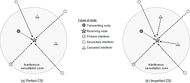
Figure 1: Effective interference model for a typical receiver canceling two strongest interferers with (a) perfect CSI or (b) imperfect CSI. The distance in the figures decreases with increasing received power. The data and interference links are plotted using solid and dashed lines, respectively.

II-F The Effective SIR Model: Imperfect CSI

Without the assumption of perfect and readily available CSI, receivers estimate the signal strength of their interferers and then identify the strongest ones by using the random training signature sequences inserted into transmitted signals [38]. Subsequently, each receiver requests their strongest interferers to transmit training sequences and uses them to estimate the corresponding interference channels. Let $M$ denote the length of each training sequence. The $L$ training sequences form an $L\times M$ matrix $\sqrt{M}{\mathbf{Q}}$ where ${\mathbf{Q}}$ consists of orthonormal row vectors [39].

Define ${\mathbf{V}}$ as an $N\times L$ matrix comprising the vectors $\{{\mathbf{h}}_{T}\mid T\in\mathcal{T}\}$ as columns. The signal ${\mathbf{Y}}$ received by $R_{0}$ during the training phase is expressed as an $N\times M$ matrix:

$${\mathbf{Y}}=\sqrt{M}{\mathbf{V}}{\mathbf{Q}}+\sum_{T\in\Phi\backslash\mathcal{T}}{\mathbf{h}}_{T}{\mathbf{x}}_{T}$$ (7)

where the factor $\sqrt{M}$ normalizes the average power of each training sequence to be one, and the $1\times M$ row vector ${\mathbf{x}}_{T}$ contains $\mathcal{CN}(0,1)$ data symbols transmitted by node $T$. The summation term in (7) represents interference to the CSI estimation at $R_{0}$. The CSI is estimated using the least-squares method to yield for every $T\in\mathcal{T}$:

$$\hat{{\mathbf{h}}}_{T} = \frac{1}{\sqrt{M}}{\mathbf{Y}}{\mathbf{q}}_{T}^{\dagger}$$ (8)

$$= {\mathbf{h}}_{T}+\frac{1}{\sqrt{M}}\sum_{T^{\prime}\in\Phi\backslash\mathcal{T}}{\mathbf{h}}_{T^{\prime}}\tilde{x}_{T^{\prime},T}$$ (9)

where ${\mathbf{q}}_{T}$ is the training sequence sent by node $T$ and $\tilde{x}_{T^{\prime},T}={\mathbf{x}}_{T}{\mathbf{q}}_{T}^{\dagger}$ has the distribution $\mathcal{CN}(0,1)$.

The SIR is derived as follows. The estimated CSI is applied for computing the beamformer ${\mathbf{v}}_{0}$ used at $R_{0}$. Using (8) and under the zero-forcing constraint: ${\mathbf{v}}_{0}^{\dagger}\hat{{\mathbf{h}}}_{T}=0$, $\forall\ T\in\mathcal{T}$, the residual interference at $R_{0}$ after beamforming, denoted as $I_{R}$, can be written as

$$I_{R} = \sum_{T\in\mathcal{T}}{\mathbf{v}}_{0}^{\dagger}{\mathbf{h}}_{T}x_{T}$$ (10)

$$= -\frac{1}{\sqrt{M}}\sum_{T\in\mathcal{T}}\sum_{T^{\prime}\in\Phi\backslash\mathcal{T}}{\mathbf{v}}_{0}^{\dagger}{\mathbf{h}}_{T^{\prime}}\tilde{x}_{T^{\prime},T}x_{T}.$$

As illustrated in Fig. 1(b), CSI estimation errors result in additional interference with respect to the case of perfect CSI. For the present case, the SIR in (6) is modified as

$$\widetilde{\mathsf{SIR}}=\frac{W}{\sigma_{R}^{2}+\sum_{T\in\Phi\backslash\mathcal{T}}I_{T}}$$ (11)

where $\sigma_{R}^{2}$ denotes the variance of $I_{R}$ in (10) conditioned on fixed $\Phi$ and channels.

III Transmission Capacity with Perfect CSI

This section focuses on the analysis of the outage probability and TC assuming prefect CSI. In particular, we derive the TC scaling with respect to the number of canceled interferers per node and the outage probability.

III-A Point Processes and Auxiliary Results

Since the $L$ strongest interferers are canceled, we refer to the $(L+1)$-st strongest interferer (in terms of pre-cancellation power) as the primary interferer and denote it as $T_{P}$, whose pre-cancellation interference power is $J_{P}=\|{\mathbf{h}}_{T_{P}}\|^{2}$. The interferers with smaller pre-cancellation interference power are referred to as the secondary interferers. There are two reasons for separating the interferers. First, considering the primary interferer alone yields a lower bound on the outage probability to be derived in the sequel. Second, as we show shortly, the secondary interferers conditioned on $J_{P}$ form a Poisson point process.

Recall that $\Phi$ stands for the homogeneous Poisson point process of all transmitters but $T_{0}$. Define a marked point process [33] $\Psi=\{(T,J_{T}\}\mid T\in\Phi\}$ where the mark of node $T$ is its pre-cancellation interference power $J_{T}$. Different interference channels are independent and hence $J_{T}$ depends on $T$ but not other points in $\Phi$. Let $\mu$ and $\mu^{*}$ denote the mean measures of $\Phi$ and $\Psi$, respectively. By applying Marking Theorem, $\Psi$ is shown to be a Poisson process on the product space $\mathds{R}^{2}\times\mathds{R}^{+}$ with mean measure $\mu^{*}$ given as [33]

$$\mu^{*}(\mathcal{B})=\iint\limits_{(t,u)\in\mathcal{B}}\mu(dt)p(t,du)$$ (12)

where $\mathcal{B}$ is a measurable subset of $\mathds{R}^{2}\times\mathds{R}^{+}$ and $p(T,\cdot)$ represents the distribution of $J_{T}$ conditioned on $T$. Let $\mathcal{G}=\mathbb{R}^{2}\times(g,\infty)$. Note that $\Psi\cap\mathcal{G}$ is the set of interferers whose pre-cancellation interference power is larger than $g$. From (12), $\mu^{*}(\mathcal{G})$ can be obtained as

$$\mu^{*}(\mathcal{G}) = \lambda\int_{t\in\mathds{R}^{2}}\int_{g}^{\infty}p(t,du)dt$$ (13)

$$= 2\pi\lambda\int_{0}^{\infty}\int_{g}^{\infty}rp(r,du)dr$$ (14)

$$= 2\pi\lambda\int_{0}^{\infty}r\Pr(J_{T}>g\mid|T|=r)dr$$ (15)

where (13) follows from the homogeneity of $\Phi$, and (14) uses polar coordinates and the fact that $J_{T}$ depends only on the distance $r_{T}=|T|$ from the origin.

Let the point process consisting of all secondary interferers conditioned on $J_{P}$ be denoted by

$$\Pi(J_{P})=\{(T,J_{T})\,|\,T\in\Phi,0\leq J_{T}<J_{P}\}.$$ (16)

The distribution of $\Pi(J_{P})$ and $J_{P}$ are characterized by the following lemmas, which are proved in Appendices -D and -E, respectively.

Lemma 1.

Conditioned on $J_{P}=g$, $\Pi(J_{P})$ is a Poisson point process on $\mathbb{R}^{2}\times[0,g)$. Its mean measure is given by

$$\mu^{*}(\mathcal{B}\mid J_{P}=g)=\lambda\iint\limits_{(t,u)\in\mathcal{B}}\mu(dt)p(t,du)$$ (17)

where $\mathcal{B}$ is a measurable subset of $\mathbb{R}^{2}\times[0,g)$ and $p(T,\cdot)$ is the distribution function of $J_{T}$ conditioned on node $T$.

Lemma 2.

The primary pre-cancellation interference power $J_{P}$ has the following cumulative distribution function

$$\Pr(J_{P}\leq g)=\sum_{k=0}^{L}\frac{\left(\nu\lambda g^{-\frac{2}{\alpha}}\right)^{k}}{\Gamma(k+1)}e^{-\nu\lambda g^{-\frac{2}{\alpha}}}$$ (18)

and the probability density function

$$f_{P}(g)=\frac{2(\nu\lambda)^{L+1}}{\alpha\Gamma(L+1)}g^{-\frac{2(L+1)}{\alpha}-1}e^{-\nu\lambda g^{-\frac{2}{\alpha}}}$$ (19)

where $\nu=\frac{\pi\Gamma(N+\frac{2}{\alpha})}{\Gamma(N)}$.

After perfect interference cancellation, the interference power of a remaining interferer $T\in\Phi\backslash\mathcal{T}$ is $I_{T}=|{\mathbf{v}}_{0}^{\dagger}{\mathbf{h}}_{T}|^{2}$. Define $\tilde{{\mathbf{h}}}_{T}={\mathbf{h}}_{T}/\|{\mathbf{h}}_{T}\|$ and $\delta_{T}=|{\mathbf{v}}_{0}^{\dagger}\tilde{{\mathbf{h}}}_{T}|^{2}$. Then $I_{T}$ and $J_{T}$ are related by $I_{T}=J_{T}\delta_{T}$. The distributions of the random variables $\{\delta_{T}\}$ are specified in the following lemma.

Lemma 3.

The set of random variables $\{\delta_{T}\mid T\in\Phi\backslash\mathcal{T}\}$ follow i.i.d. beta$(1,N-1)$ distributions as specified by the following probability density function

$$f_{\delta}(x)=(N-1)(1-x)^{N-2},\quad x\in(0,1).$$ (20)

Furthermore, $\delta_{T}$ is independent with $J_{T}$.

Proof: See Appendix -F.  $\Box$

It follows that the primary interference power $I_{P}$ is given as $I_{P}=J_{P}\delta_{P}$ where $\delta_{P}$ is a beta$(1,N-1)$ random variable. Given that $\delta_{P}$ is random, node $T_{P}$ may not contribute the largest interference power despite its dominance over other uncanceled interferers in terms of pre-cancellation interference power. Next, the total secondary interference power can be written as $I_{S}=\sum_{T\in\Phi\backslash(\mathcal{T}\cup\{T_{P}\})}J_{T}\delta_{T}$. This summation is a type of shot noise [33] whose probability density function has no known closed-form expression except for some simple cases [32, 2]. Nevertheless, the conditional first and second moments of $I_{S}$ can be obtained as shown in the following lemma.

Lemma 4.

After perfect spatial interference cancellation, the secondary interference power $I_{S}$ conditioned on the primary pre-cancellation interference power $J_{P}=g$ has the following mean and variance

$$\mathbb{E}[I_{S}\,|\,J_{P}=g] = \frac{2\nu\lambda}{N(\alpha-2)}g^{1-\frac{2}{\alpha}}$$ (21)

$$\mathsf{var}(I_{S}\,|\,J_{P}=g) = \frac{2\nu\lambda}{N(N+1)(\alpha-1)}g^{2-\frac{2}{\alpha}}.$$ (22)

Proof: See Appendix -G.  $\Box$

III-B Bounds on Outage Probability

From (6), the outage probability $P_{\mathsf{out}}$ can be written as

$$P_{\mathsf{out}}=\Pr(I_{S}+I_{P}>W\theta^{-1}).$$ (23)

It follows that $P_{\mathsf{out}}$ can be lower bounded as

$$P_{\mathsf{out}}\geq\Pr(I_{P}>W\theta^{-1})$$ (24)

by considering only the primary interferer, which is tight if the primary interfererence is dominant. Using $I_{P}=J_{P}\delta_{P}$ and (23), an upper bound on $P_{\mathsf{out}}$ is obtained as

$$P_{\mathsf{out}} \leq \Pr(I_{S}+J_{P}>W\theta^{-1})$$ (25)

$$= \Pr(J_{P}>W\theta^{-1})+\Pr(I_{S}>W\theta^{-1}-J_{P}\mid J_{P}\leq W\theta^{-1})\Pr(J_{P}\leq W\theta^{-1})$$ (26)

where (25) holds since $\delta_{P}\leq 1$. The above upper bound can be further bounded by applying the following Chebyshev’s inequality:

$$\Pr(I_{S}\geq a\mid J_{P}=g)\leq\min\left\{\frac{\mathsf{var}(I_{S}\,|\,J_{P}=g)}{\left\{a-\mathbb{E}\left[I_{S}\,|\,J_{P}=g\right]\right\}^{2}},1\right\},\quad\forall\ a>\mathbb{E}\left[I_{S}\,|\,J_{P}=g\right].$$ (27)

Based on (24), (26) and (27), bounds on the outage probability are derived as shown in the following lemma.

Lemma 5.

For perfect spatial interference cancellation, the outage probability satisfies $P_{\mathsf{out}}^{\ell}(\lambda)\leq P_{\mathsf{out}}\leq P_{\mathsf{out}}^{u}(\lambda)$ where:

1. The lower bound is

   $$P_{\mathsf{out}}^{\ell}(\lambda)=1-\sum_{k=0}^{L}\frac{\left(\nu\lambda\theta^{\frac{2}{\alpha}}\right)^{k}}{\Gamma(k+1)}\mathbb{E}\left[\left(\frac{W}{\delta_{P}}\right)^{-\frac{2k}{\alpha}}e^{-\nu\lambda\theta^{\frac{2}{\alpha}}\left(\frac{W}{\delta_{P}}\right)^{-\frac{2}{\alpha}}}\right].$$ (28)

2. Define the subsets $\mathcal{D}_{1}$ and $\mathcal{D}_{2}$ of the product space $\mathds{R}^{+}\times\mathds{R}^{+}$ as

   $$\mathcal{D}_{1} = \left\{(w,g)\mid w\theta^{-1}-\mathbb{E}[I_{S}\mid J_{P}=g]\leq g\leq w\theta^{-1}\right\}$$ (29)

   $$\mathcal{D}_{2} = \left\{(w,g)\mid g<w\theta^{-1}-\mathbb{E}[I_{S}\mid J_{P}=g]\right\}.$$ (30)

   The upper bound is

   $$P_{\mathsf{out}}^{u}(\lambda)=\Lambda_{1}+\Lambda_{2}+\Lambda_{3}$$ (31)

   where

   $$\Lambda_{1} =1-\sum_{k=0}^{L}\frac{\left(\nu\lambda\theta^{\frac{2}{\alpha}}\right)^{k}}{\Gamma(k+1)}\mathbb{E}\left[W^{-\frac{2k}{\alpha}}e^{-\nu\lambda\theta^{\frac{2}{\alpha}}W^{-\frac{2}{\alpha}}}\right]$$ (32)

   $$\Lambda_{2} =\iint\limits_{(w,g)\in\mathcal{D}_{1}}f_{W}(w)f_{P}(g)dwdg$$ (33)

   $$\Lambda_{3} =\iint\limits_{(w,g)\in\mathcal{D}_{2}}\min\left\{\frac{\mathsf{var}(I_{S}\,|\,J_{P}=g)}{\left\{w\theta^{-1}-g-\mathbb{E}\left[I_{S}\,|\,J_{P}=g\right]\right\}^{2}},1\right\}f_{W}(w)f_{P}(g)dwdg$$ (34)

   with $\mathbb{E}(I_{S}\,|\,J_{P}=g)$ and $\mathsf{var}(I_{S}\,|\,J_{P}=g)$ given in Lemma 4.

Proof: See Appendix -H.  $\Box$

III-C Asymptotic Transmission Capacity

Using the upper and lower bounds described in Lemma 5, the TC scaling is analyzed for a large number of canceled interferers per node ($L\rightarrow\infty$) or varnishing outage probability ($\epsilon\rightarrow 0$) as follows.

Increasing the number of antennas at each receiver allows more interferers to be canceled, leading to higher TC. The TC scaling as $L\rightarrow\infty$ is given in the following theorem.

Theorem 1.

With perfect CSI and fixed array gain $(N-L)$, if the number of canceled interferers per node $L$ is sufficiently large, the transmission capacity is bounded as

$$\frac{1}{\pi}\left[\frac{\epsilon\left(\alpha-2\right)}{2\theta\mathbb{E}[W^{-1}]}\right]^{\frac{2}{\alpha}}\leq\frac{C(L)}{(1-\epsilon)\log_{2}(1+\theta)L^{1-\frac{2}{\alpha}}}\leq\frac{2}{\pi}\left[\frac{\mathbb{E}[W]}{\theta(1-\epsilon)}\right]^{\frac{2}{\alpha}}.$$ (35)

Proof: See Appendix -I.  $\Box$

The relationship in (35) shows that TC grows in the order of $L^{1-2/\alpha}$, where the growth is faster for steeper path loss. Intuitively, if interference decays more quickly with distance, canceling the strongest interferers reduces interference more significantly.

Small target outage probability results in a network of sparse transmitting nodes (i.e., $\lambda\rightarrow 0$). For such a sparse network, the relationship between the outage probability and node density is given in the following lemma.

Lemma 6.

With perfect CSI and $\lambda\rightarrow 0$, the outage probability is bounded as follows.

1. If $L+1\leq\alpha$, for sufficiently small $\lambda$,

   $$\kappa_{1}\leq\frac{\epsilon}{\lambda^{L+1}}\leq\kappa_{2}$$ (36)

   where

   $$\kappa_{1} = \frac{E\left[\delta_{P}^{\frac{2}{\alpha}(L+1)}\right]E\left[W^{-\frac{2}{\alpha}(L+1)}\right]\left(\nu\theta^{\frac{2}{\alpha}}\right)^{L+1}}{\Gamma(L+2)}$$ (37)

   $$\kappa_{2} = \frac{2^{\frac{2}{\alpha}(L+1)+1}\mathbb{E}\left[W^{-\frac{2}{\alpha}(L+1)}\right](\nu\theta^{\frac{2}{\alpha}})^{L+1}}{\Gamma(L+2)}.$$ (38)

2. If $L+1>\alpha$, for sufficiently small $\lambda$,

   $$\kappa_{1}\leq\frac{\epsilon}{\lambda^{L+1}}\quad\textrm{and}\quad\frac{\epsilon}{\lambda^{\alpha}}\leq\kappa_{3}$$ (39)

   where

   $$\kappa_{3}=\frac{8\theta^{2}\nu^{\alpha}\Gamma(L-\alpha+2)\mathbb{E}[W^{-2}]}{N(N+1)(\alpha-1)\Gamma(L+1)}.$$ (40)

Proof: See Appendix -J.  $\Box$

Note that the ratio $\frac{\kappa_{2}}{\kappa_{1}}$ decreases as $L$ becomes smaller. This suggests that the asymptotic bounds are tighter for smaller values of $L$.

Using Lemma 6 and the TC definition in (1), we have the following TC scaling.

Theorem 2.

With perfect CSI and small target outage probability $\epsilon\rightarrow 0$, the TC is bounded as follows.

1. If $L+1\leq\alpha$, for sufficiently small $\epsilon$,

   $$\kappa_{2}^{-\frac{1}{L+1}}\leq\frac{C(\epsilon)}{\log(1+\theta)\epsilon^{\frac{1}{L+1}}}\leq\kappa_{1}^{-\frac{1}{L+1}}$$ (41)

   where $\kappa_{1}$ and $\kappa_{2}$ are given in Lemma 6.

2. If $L+1>\alpha$, for sufficiently small $\epsilon$,

   $$\kappa_{3}^{-\frac{1}{\alpha}}\leq\frac{C(\epsilon)}{\log_{2}(1+\theta)\epsilon^{\frac{1}{\alpha}}}\quad\textrm{and}\quad\frac{C(\epsilon)}{\log_{2}(1+\theta)\epsilon^{\frac{1}{L+1}}}\leq\kappa_{1}^{-\frac{1}{L+1}}$$ (42)

   where $\kappa_{3}$ is given in Lemma 6.

The above theorem shows that as $\epsilon$ decreases, $C(\epsilon)$ follows a power law. For $L+1>\alpha$, only bounds on the exponent are known. The derivation of the exact scaling for $L+1>\alpha$ requires a tighter upper bound on outage probability than that based on Chebyshev’s inequality in (27). This may require analyzing the distribution function of the secondary interference power, which, however, has no known closed-form expression for the present case.

For $L+1\leq\alpha$, the exponent of the TC power law is $1/(L+1)$. This power law indicates that $L$ determines the sensitivity of TC to a change in the outage constraint. To facilitate our discussion, rewrite the scaling in Theorem 2 as $C(\epsilon)\cong\alpha\epsilon^{\frac{1}{L+1}}$ where “$\cong$” represents asymptotic equivalence for $\epsilon\rightarrow 0$. The sensitivity of TC towards changes of the outage constraint decreases inversely with the number of canceled interferers. Reducing the outage probability by two orders of magnitude decreases the TC by $10$, $3.2$, and $1.8$-fold in the case of $1$, $3$ and $7$ canceled interferers per node, respectively. Last, from simulation results in Section V, the TC scaling in Theorem 2 is observed to also hold for outage probabilities of practical interest ($\epsilon\leq 0.1$).

According to Theorem 2, the decay rate of the TC with varnishing outage probability can be slowed down by employing more antennas for interference cancellation at the cost of increasing CSI estimation overhead, which can be considered as overhead for local coordination among nearby nodes. However, to guarantee nonzero network capacity for zero outage probability, perhaps the better choice is to rely on centralized scheduling as in [16]. Nevertheless, such scheduling requires global coordination and potentially incurs much higher overhead than combining the random access protocol and spatial interference cancellation. Thus the current setup balances network performance and overhead.

IV Transmission Capacity with Imperfect CSI

This section addresses the effect of imperfect CSI. First, consider the scenario where the network remains unchanged except that the CSI is imperfect and the users have to relax their quality-of-service (QoS) requirements, namely to tolerate higher outage probability represented by $\tilde{P}_{\mathsf{out}}$ and to lower the date rate from $\log_{2}(1+\theta)$ to $\log_{2}(1+\tilde{\theta})$, where $\tilde{\theta}$ denote the corresponding SIR threshold. Thus $\tilde{P}_{\mathsf{out}}=\Pr(\widetilde{\mathsf{SIR}}\leq\tilde{\theta})$ where $\widetilde{\mathsf{SIR}}$ is given in (11). The corresponding TC is

$$\tilde{C}=(1-\tilde{P}_{\mathsf{out}})\log_{2}(1+\tilde{\theta})\lambda.$$ (43)

It is interesting to investigate the required training sequence length under a constraint on the QoS degradation. To this end, define

$$\Delta P =\tilde{P}_{\mathsf{out}}(\tilde{\theta})-P(\theta)$$ (44)

$$\Delta B =\log_{2}(1+\theta)-\log_{2}(1+\tilde{\theta})$$ (45)

$$\Delta C =C-\tilde{C}.$$ (46)

We consider the following constraints on the QoS degradation: $\Delta P\leq\vartheta_{p}$ and $\Delta B\leq\vartheta_{b}$ with $\vartheta_{p},\vartheta_{b}\geq 0$. The training sequence length that satisfies these constraints and the corresponding TC loss, specified by the ratio $\frac{\Delta C}{C}$, are shown in the following theorem.

Theorem 3.

To satisfy the constraints $\Delta P\leq\vartheta_{p}$ and $\Delta B\leq\vartheta_{b}$, it is sufficient to choose the training-sequence length as

$$M=\max\left(\left\lceil\frac{\log L-\log\vartheta_{p}}{\omega(2^{\vartheta_{b}}-1)}\right\rceil,L\right)$$ (47)

with $\omega=\left[\Gamma(L+1)\right]^{-\frac{1}{L}}$. Moreover, the resultant TC loss normalized by $C$ is bounded as

$$\frac{\Delta C}{C}\leq\frac{\vartheta_{p}}{1-\epsilon}+\frac{\vartheta_{b}}{\log_{2}(1+\theta)}.$$ (48)

Proof: See Appendix -K.  $\Box$

Note that (47) takes into account that $M\geq L$ (see Section II-F) and $M$ is an integer. For stringent constraints $\vartheta_{p}\rightarrow 0$ and $\vartheta_{b}\rightarrow 0$, it can be observed from (47) that the training sequence length is approximately proportional to $\log\frac{1}{\vartheta_{p}}$ and $\frac{1}{\vartheta_{b}}$. Also, the upper-bound in (48) suggests that the normalized capacity loss is more sensitive to the variation of $\vartheta_{p}$ if $\epsilon$ is large and $\vartheta_{b}$ if $\log_{2}(1+\theta)$ is small.

Next, for small outage probability, the required training sequence length is derived for achieving the same TC scaling as for perfect CSI given identical QoS requirements. These results are shown in the following theorem.

Theorem 4.

For $\epsilon\rightarrow 0$ and $\Delta B\overset{\epsilon}{\rightarrow}0$, $\Delta P\overset{\epsilon}{\rightarrow}0$,, the following scaling of the training sequence length

$$\lim_{\epsilon\rightarrow 0}\frac{M}{\frac{1+\varrho}{\omega}\epsilon^{-\varrho}}=1$$ (49)

with an arbitrary $\varrho>0$ is sufficient for achieving the transmission-capacity scaling for perfect CSI as given in Theorem 2.

Proof: See Appendix -L.  $\Box$

The above theorem shows that to achieve the optimal asymptotic TC, $M$ increases slowly (sub-linearly with an arbitrary positive exponent) with $\frac{1}{\epsilon}$, indicating small CSI estimation overhead. The reason is that CSI inaccuracy rises mainly from weak interferers and thus its effect is moderate.

Suppose the CSI estimation process repeats for every channel coherence time $t_{c}$ (in symbols). The overhead of CSI estimation can be regarded as the TC decrease by a factor of $M/t_{c}$. Simulation results in Fig. 6 reveal that the capacity gain from interference cancellation results mostly from canceling only a few strongest interferers and thus $L$ can be kept small; furthermore, short training sequences (small $M$) are sufficient for approaching the TC achieved with perfect CSI. Thus, the overhead is insignificant if mobility is low (large $t_{c}$).

V Simulation and Discussion

In this section, the bounds on outage probability and TC are evaluated using Monte Carlo simulation. The procedure for simulating a MANET follows that in [40]. The simulated ad hoc network lies on a two-dimensional disk and contains a number of transmitter-receiver pairs, which is a Poisson random variable with the mean equal to $200$. The disk area is adjusted according to the node density. The typical receiver is placed at the center of the disk. We set the required SIR as $\theta=3$ or $4.8$ dB, the link array gain $(N-L)=2$, and the path-loss exponent as $\alpha=4$ unless specified otherwise.

V-A Bounds on Outage Probability

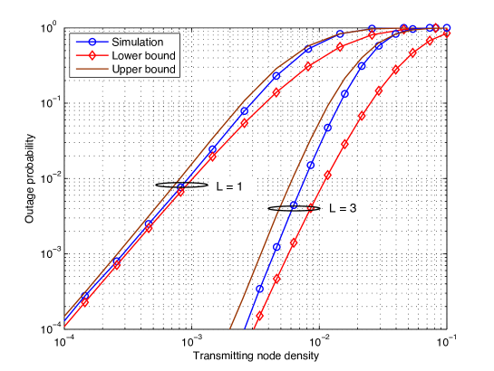
Figure 2: Outage probability for different transmitting node densities and perfect CSI.

For perfect CSI, the bounds on outage probability from Lemma 5 and simulated values are compared in Fig. 2. It can be observed that the outage probability is approximately proportional to $\lambda^{L+1}$. The bounds for $L=1$ are tighter than those for $L=3$. Moreover, the bounds on outage probability converge to the exact values as the transmitting node density $\lambda$ decreases. These two observations can be explained by the dominance of the primary interference over the secondary one as $L$ or $\lambda$ decreases, where the secondary interference causes the looseness of the bounds on outage probability.

In Fig. 3, given identical data rates ($\Delta B=0$), the outage probability for imperfect CSI is observed to rapidly converge to the perfect-CSI counterpart as $M$ increases. In particular, for $M=11$, CSI inaccuracy increases outage probability by less than two-fold.

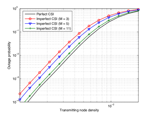
Figure 3: Compare outage probability for perfect and imperfect CSI given different transmitting node densities. The training-sequence length is $M=\{3,5,11\}$ and the number of canceled interferers per node is $L=3$.

V-B Scaling of Transmission Capacity

In Fig. 4, asymptotic bounds on TC in Theorem 2 are compared with the exact values obtained by simulation for perfect CSI and the range of target outage probability $\epsilon\in[10^{-5},10^{-1}]$. The corresponding curves are identified using the legends “asymptotic upper bound”, “asymptotic lower bound”, and “simulation”. Different combinations of $(L,\alpha)$ are separated according to the cases of $L+1\leq\alpha$ and $L+1>\alpha$, corresponding to Fig. 4(a) and Fig. 4(b), respectively. As observed from Fig. 4(a), for $L+1\leq\alpha$, the asymptotic upper bound on TC is tight even in the non-asymptotic range e.g., $\epsilon\in[0.01,0.1]$. The tightness of this bound is due to the dominance of primary interference when $L$ is small. Moreover, Fig. 4(b) shows that for $L+1>\alpha$ the slopes of the “simulation” curves converge to those of the corresponding “asymptotic upper bound” curves as the target outage probability decreases. The above observations suggest that for both $L+1\leq\alpha$ and $L+1>\alpha$, the TC scaling for small target outage probability follows the power law with the same exponent $\frac{1}{L+1}$.

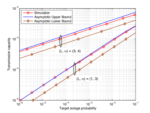
(a) $L+1\leq\alpha$

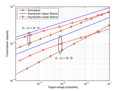
(b) $L+1>\alpha$

Figure 4: Comparison between asymptotic bounds on TC and the exact values obtained by simulation for perfect CSI and the cases of (a) $L+1\leq\alpha$ and (b) $L+1>\alpha$.

V-C Transmission Capacity vs. Size of Antenna Array

In Fig. 5, the transmission capacity is plotted for an increasing number of canceled interferers per node assuming perfect CSI. Furthermore, different target outage probabilities, namely $\epsilon=\{10^{-1},10^{-2},10^{-3}\}$, are considered. As observed from Fig. 5, the cancellation of a few interferers by each node leads to a TC gain of an order of magnitude or more with respect to the case of no cancellation. For example, for $\epsilon=10^{-2}$, canceling two interferers per node provides a $25$-time TC gain. The cancellation of more interferers has a diminishing effect on the network capacity since it becomes limited by secondary interference. It is also observed that the outage constraint affects TC more significantly for smaller $L$.

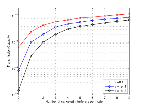
Figure 5: Transmission capacity by simulation for different node densities and perfect CSI. The target outage probability is $\epsilon=\{10^{-1},10^{-2},10^{-3}\}$.

The effect of imperfect CSI on TC is shown in Fig. 6, where TC is plotted for increasing $L$. The TC loss due to CSI estimation errors is observed to reduce as $M$ increases. Such a loss is relatively small even for a moderate value of $M$. For instance, the TC reduction is $25$% for $M=11$ and $L=7$. Next, even for small $M$ (i.e., $M=3$), a TC gain of more than an order of magnitude can be achieved by interference cancellation. This confirms the practicality of interference cancellation.

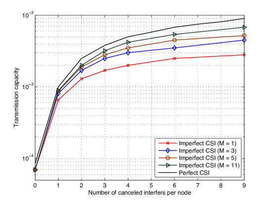
Figure 6: Transmission capacity by simulation for different node densities and imperfect CSI. The target outage probability is $\epsilon=10^{-2}$.

References

- [1] S. P. Weber, X. Yang, J. G. Andrews, and G. de Veciana, “Transmission capacity of wireless ad hoc networks with outage constraints,” IEEE Trans. on Inform. Theory, vol. 51, pp. 4091–4102, Dec. 2005.
- [2] S. P. Weber, J. G. Andrews, and N. Jindal, “The effect of fading, channel inversion, and threshold scheduling on ad hoc networks,” IEEE Trans. on Inform. Theory, vol. 53, pp. 4127–4149, Nov. 2007.
- [3] A. Hasan and J. G. Andrews, “The guard zone in wireless ad hoc networks,” IEEE Trans. on Wireless Communications, vol. 6, pp. 897–906, Mar. 2007.
- [4] R. K. Ganti and M. Haenggi, “Regularity, interference, and capacity of large ad hoc networks,” in Proc., IEEE Asilomar, Oct. 2006.
- [5] J. Venkataraman, M. Haenggi, and O. Collins, “Shot noise models for the dual problems of cooperative coverage and outage in random networks,” in Proc., Allerton Conf. on Comm., Control, and Computing, Sept. 2006.
- [6] N. Jindal, J. G. Andrews, and S. P. Weber, “Bandwidth partitioning in decentralized wireless networks,” IEEE Trans. on Wireless Communications, vol. 7, pp. 5408–5419, Jul. 2008.
- [7] S. P. Weber, J. G. Andrews, X. Yang, and G. de Veciana, “Transmission capacity of wireless ad hoc networks with successive interference cancelation,” IEEE Trans. on Inform. Theory, vol. 53, pp. 2799–2814, Aug. 2007.
- [8] A. M. Hunter, J. G. Andrews, and S. P. Weber, “Transmission capacity of ad hoc networks with spatial diversity,” IEEE Trans. on Wireless Communications, vol. 7, pp. 5058–5071, Dec. 2008.
- [9] M. Haenggi, J. G. Andrews, F. Baccelli, O. Dousse, and M. Franceschetti, “Stochastic geometry and random graphs for the analysis and design of wireless networks,” IEEE Journal on Selected Areas in Communications, vol. 27, pp. 1029–1046, Jul. 2009.
- [10] K. Huang, J. G. Andrews, R. W. Heath, Jr., D. Guo, and R. A. Berry, “Spatial interference cancelation for mobile ad hoc networks: Imperfect CSI,” in Proc., IEEE Asilomar, pp. 131–135, Oct. 2008.
- [11] K. Huang, J. G. Andrews, R. W. Heath, Jr., D. Guo, and R. A. Berry, “Spatial interference cancelation for mobile ad hoc networks: Perfect CSI,” in Proc., IEEE Globecom, pp. 1–5, Nov. 2008.
- [12] R. H. Y. Louie, M. R. McKay, and I. B. Collings, “Spatial multiplexing and diversity communications in ad hoc networks,” to appear in IEEE Trans. on Inform. Theory.
- [13] M. Kountouris and J. G. Andrews, “Transmission capacity scaling of SDMA in wireless ad hoc networks,” in Proc., Information Theory Workshop, pp. 534–538, Oct. 2009.
- [14] R. Vaze and R. W. Heath Jr., “Optimal use of multiple antennas in ad-hoc networks : Transmission capacity perspective,” submitted to IEEE Trans. on Inform. Theory.
- [15] N. Jindal, J. G. Andrews, and S. Weber, “Multi-antenna communication in ad hoc networks: achieving MIMO gains with SIMO transmission,” submitted to IEEE Trans. on Communications.
- [16] P. Gupta and P. R. Kumar, “The capacity of wireless networks,” IEEE Trans. on Inform. Theory, vol. 46, pp. 388–404, Mar. 2000.
- [17] V. R. Cadambe and S. A. Jafar, “Interference alignment and the degrees of freedom for the K user interference channel,” IEEE Trans. on Inform. Theory, vol. 54, pp. 3425–3441, Aug. 2008.
- [18] M. Zorzi, J. Zeidler, A. Anderson, B. Rao, J. Proakis, A. L. Swindlehurst, M. Jensen, and S. Krishnamurthy, “Cross-layer issues in MAC protocol design for MIMO ad hoc networks,” IEEE Wireless Communications Magazine, vol. 13, pp. 62–76, Aug. 2006.
- [19] B. Hamdaoui and K. G. Shin, “Characterization and analysis of multi-hop wireless MIMO network throughput,” in Proc., Intl. Symp. on Mobile Ad Hoc Networking and Computing, pp. 120–129, 2007.
- [20] J. C. Mundarath, P. Ramanathan, and B. D. V. Veen, “A cross layer scheme for adaptive antenna array based wireless ad hoc networks in multipath environments,” Wireless Networks, vol. 13, no. 5, pp. 597–615, 2007.
- [21] J.-S. Park, A. Nandan, M. Gerla, and H. Lee, “SPACE-MAC: enabling spatial reuse using MIMO channel-aware MAC,” in Proc., IEEE Intl. Conf. on Communications, vol. 5, pp. 3642–3646, May 2005.
- [22] M. Z. Siam, M. Krunz, A. Muqattash, and S. Cui, “Adaptive multi-antenna power control in wireless networks,” in Proc., Intl. Conf. on Wireless Comm. and Mobile Computing, pp. 875–880, Jul. 2006.
- [23] R. Ramanathan, J. Redi, C. Santivanez, D. Wiggins, and S. Polit, “Ad hoc networking with directional antennas: a complete system solution,” IEEE Journal on Selected Areas in Communications, vol. 23, pp. 496–506, Mar. 2005.
- [24] A. Deopura and A. Ganz, “Provisioning link layer proportional service differentiation in wireless networks with smart antennas,” Wireless Networks, vol. 13, Mar. 2007.
- [25] K. Sundaresan and R. Sivakumar, “A unified MAC layer framework for ad-hoc networks with smart antennas,” IEEE Trans. on Networking, vol. 15, pp. 546–559, Mar. 2007.
- [26] H. Singh and S. Singh, “Smart-ALOHA for multi-hop wireless networks,” Mobile Networks and Applications, vol. 10, pp. 651–662, May 2005.
- [27] R. Ramanathan, “On the performance of ad hoc networks with beamforming antennas,” in Proc., Intl. Symp. on Mobile Ad Hoc Networking and Computing, pp. 95–105, Oct. 2001.
- [28] Y. Wu, L. Zhang, Y. Wu, and Z. Niu, “Interest dissemination with directional antennas for wireless sensor networks with mobile sinks,” in Proc., Intl. Conf. on Embedded Networked Sensor Systems, pp. 99–111, Nov. 2006.
- [29] S. Kumar, V. S. Raghavan, and J. Deng, “Medium access control protocols for ad hoc wireless networks: A survey,” Ad Hoc Networks, vol. 4, pp. 326–358, May 2006.
- [30] J. Zhang and S. C. Liew, “Capacity improvement of wireless ad hoc networks with directional antennae,” SIGMOBILE Mobile Computing Comm. Review, vol. 10, Apr. 2006.
- [31] S. Yi, Y. Pei, S. Kalyanaraman, and B. Azimi-Sadjadi, “How is the capacity of ad hoc networks improved with directional antennas?,” Wireless Networks, vol. 13, no. 5, pp. 635–648, 2007.
- [32] F. Baccelli, B. Blaszczyszyn, and P. Muhlethaler, “An ALOHA protocol for multihop mobile wireless networks,” IEEE Trans. on Inform. Theory, vol. 52, pp. 421–36, Feb. 2006.
- [33] J. F. C. Kingman, Poisson processes. Oxford University Press, 1993.
- [34] D. Stoyan, W. S. Kendall, and J. Mecke, Stochastic Gemoetry and its Applications. Wiley, 2nd ed., 1995.
- [35] J. G. Andrews, S. Weber, M. Kountouris, and M. Haenggi, “Random access transport capacity,” IEEE Trans. on Wireless Communications, vol. 9, pp. 2101–2111, Jun. 2010.
- [36] T. K. Y. Lo, “Maximum ratio transmission,” IEEE Trans. on Communications, vol. 47, pp. 1458–1461, Oct. 1999.
- [37] A. Paulraj, R. Nabar, and D. Gore, Introduction to Space-Time Wireless Communications. Cambridge University Press, 2003.
- [38] S. Verdu, Multiuser Detection. Cambridge, UK: Cambridge, 1998.
- [39] T. L. Marzetta and B. M. Hochwald, “Fast transfer of channel state information in wireless systems,” IEEE Trans. on Sig. Proc., vol. 54, pp. 1268–1278, Apr. 2006.
- [40] S. P. Weber and M. Kam, “Computational complexity of outage probability simulations in mobile ad-hoc networks,” in Proc., Conf. on Information Sciences and Systems, Mar. 2005.
- [41] C. K. Au-Yeung and D. J. Love, “On the performance of random vector quantization limited feedback beamforming in a MISO system,” IEEE Trans. on Wireless Communications, vol. 6, pp. 458–462, Feb. 2007.
- [42] I. Gradshteyn and I. Ryzhik, Table of integrals, series, and products. Academic Press, 7 ed., 2007.
- [43] D. Kershaw, “Some extensions of W. Gautschi’s inequalities for the Gamma function,” Math. of Computation, vol. 41, pp. 607–611, Oct. 1983.
- [44] H. Alzer, “On some inequalities for the incomplete Gamma function,” Mathematics of Computation, vol. 66, pp. 771–778, Apr. 2005.