A study of two-qubit density matrices with fermionic purifications

Abstract

We study $12$ parameter families of two qubit density matrices, arising from a special class of two-fermion systems with four single particle states or alternatively from a four-qubit state with amplitudes arranged in an antisymmetric matrix. We calculate the Wooters concurrences and the negativities in a closed form and study their behavior. We use these results to show that the relevant entanglement measures satisfy the generalized Coffman-Kundu-Wootters formula of distributed entanglement. An explicit formula for the residual tangle is also given. The geometry of such density matrices is elaborated in some detail. In particular an explicit form for the Bures metric is given.

I Introduction

Entanglement is the basic resource of quantum information processingNielsen . As such it has to be quantified and its structure characterized. For entanglement quantification one uses special classes of entanglement measures which are real-valued functions on the states. Pure and mixed state entanglement and its quantification in its bipartite form is a well-understood phenomenon. Moreover, on the geometry and structure of entangled states associated with such systems a large number of interesting results is availableGeom .

For example for pure states of bipartite systems the classification of different entanglement types is effected by the Schmidt decomposition. If the Schmidt decomposition is known, from the Schmidt numbers one can form the von-Neumann entropyPetz as a good measure characterizing bipartite entanglement. For quantifying mixed state entanglement no such general method exists. For the special case of two qubits as a measure of entanglement we have the celebrated formula of Hill and WoottersHill for the bipartite concurrence ${\cal C}$ and the associated entanglement of formation. The structure of this measure of entanglement was studied in many different papershivatbengtsson . Its structure has been related to antilinear operatorsUhlmann , combs and filtersSiewert , and has also been generalized to rebitsFuchs . Explicit expressions for different special classes of density matrices and a comparison with other measures of entanglement has been givenEisert ; Verstraete ; Ishizaka .

In this paper we would like to study the structure of special $12$ parameter families of two-qubit density matrices for which the the mixed state concurrences can be calculated in a closed form. Such density matrices can be regarded as reduced ones coming from some larger system with special properties. In order to motivate our choice for this larger system we consider an example. If we consider a three-qubit state $|\psi\rangle\in\mathbf{C}^{2}\otimes\mathbf{C}^{2}\otimes\mathbf{C}^{2}$, then after calculating any of the reduced density matrices e.g. ${\varrho}_{12}={\rm Tr}_{3}(|\psi\rangle\langle\psi|)$ we are left with a two-qubit density matrix of very special structure. For example in this case ${\varrho}_{12}$ is of rank two, and this observation enables an explicit calculation of the mixed state concurrence in terms of the amplitudes of the three-qubit state $|\psi\rangle$. This result forms the basis of further important developments namely the derivation of the Coffman-Kundu-Wootters relation of distributed entanglementKundu .

Proceeding by analogy we expect that four-qubit states of special structure might provide us with further interesting examples of that kind. Let us consider a four-qubit state $|\Psi\rangle\in\mathbf{C}^{2}\otimes\mathbf{C}^{2}\otimes\mathbf{C}^{2}\otimes\mathbf{C}^{2}$. A class of two-qubit density matrices arises after forming the reduced density matrices like ${\varrho}_{12}={\rm Tr}_{34}(|\Psi\rangle\langle\Psi|)$. However, density matrices of that kind are still too general to have a characteristic structure. Hence as an extra constraint we impose an antisymmetry condition on the amplitudes of

$$|\Psi\rangle=\sum_{ijkl=0}^{1}{\Psi}_{ijkl}|ijkl\rangle,$$ (1)

as

$${\Psi}_{ijkl}=-{\Psi}_{klij},$$ (2)

i.e. we impose antisymmetry in the first and second pairs of indices.

An alternative (and more physical) way is the one of imposing such constraints on the original Hilbert space $H\simeq\mathbf{C}^{16}$ which renders to have a tensor product structure on one of its six dimensional subspaces ${\cal H}$ of the form

$${\cal H}=(\mathbf{C}^{2}\otimes\mathbf{C}^{2})\wedge(\mathbf{C}^{2}\otimes\mathbf{C}^{2}),$$ (3)

where $\wedge$ refers to antisymmetrization. As we know quantum tensor product structures are observable-inducedZanardi , hence in order to specify our system with a tensor product structure of Eq. (3) we have to specify the experimentally accessible interactions and measurements that account for the admissible operations we can perform on our system. For example we can realize our system as a pair of fermions with four single particle states where a part of the admissible operations are local unitary transformations of the form

$$|\Psi\rangle\mapsto(U\otimes V)\otimes(U\otimes V)|\Psi\rangle,\qquad U,V\in U(2),\qquad|\Psi\rangle\in{\cal H}.$$ (4)

Taken together with Eq. (2) this transformation rule clearly indicates that the first and the second and the third and fourth subsystems form two indistinguishable subsystems of fermionic type.

The aim of the present paper is to study the interesting structure of the reduced density matrices of the form ${\varrho}_{ij},\quad i<j,\quad i,j=1,2,3,4$ arising from fermionic states that are elements of the tensor product structure as shown by Eq. (3). We can alternatively coin the term that these density matrices are ones with fermionic purifications.

The organization of the paper is as follows. In Section II. we present our parametrized family of density matrices we wish to study. Using suitable local unitary transformations we transform this family to a canonical form. In Section III. based on these results we calculate the Wootters concurrence the negativity and the purity. We give a formula for the upper bound of negativity for a given concurrence. (We prove it in Appendix A.) In section IV. we analyze the structure of these quantities and discuss how they are related to each other. In particular we prove that the relevant entanglement measures associated with our four-qubit state satisfy the generalized Coffman-Kundu-Wootters inequality of distributed entanglementOsborne . For the residual tangle we derive an explicit formula, containing two from the four algebraically independent four-qubit invariants. In Section V. we investigate the Bures geometry of this special subclass of two-qubit density matrices. We show that thanks to our purifications being fermionic an explicit formula for the Bures metric with hyperbolic structure can be obtained. The conclusions and some comments are left for Section VI.

II The density matrix

Let us parametrize the $6$ amplitudes of our normalized four qubit state $|\Psi\rangle$ of Eq. (1) with the antisymmetry property of Eq. (2) as

$$\Psi_{ijkl}=\frac{1}{2}\left({\varepsilon}_{ik}{\cal A}_{jl}+{\cal B}_{ik}{\varepsilon}_{jl}\right),$$ (5)

where ${\cal A}$ and ${\cal B}$ are symmetric matrices of the form

$${\cal A}=\begin{pmatrix}z_{1}-iz_{2}&-z_{3}\\ -z_{3}&-z_{1}-iz_{2}\end{pmatrix}=\varepsilon({\bf z}\overline{\boldsymbol{\sigma}}),\quad{\cal B}=\begin{pmatrix}w_{1}-iw_{2}&-w_{3}\\ -w_{3}&-w_{1}-iw_{2}\end{pmatrix}=\varepsilon({\bf w}\overline{\boldsymbol{\sigma}}),$$ (6)

where ${\bf z},{\bf w}\in\mathbf{C}^{3}$, $\mathbf{w}{\boldsymbol{\sigma}}=w_{1}\sigma_{1}+w_{2}\sigma_{2}+w_{3}\sigma_{3}$, with the usual $\sigma_{i}$ Pauli matrices,

$$\varepsilon=\begin{pmatrix}0&1\\ -1&0\end{pmatrix}$$ (7)

and the overline refers to complex conjugation.

It is straightforward to check, that the normalization condition of the state $|\Psi\rangle$ takes the form:

$$\|\Psi\|^{2}\equiv\|\mathbf{w}\|^{2}+\|\mathbf{z}\|^{2}:=1$$ (8)

The density matrices we wish to study are arising as reduced ones of the form

$$\varrho\equiv\varrho_{12}={\rm Tr}_{34}(|\Psi\rangle\langle\Psi|).$$ (9)

Notice that since the $(12)$ and $(34)$ subsystems are by definition indistinguishable we also have $\varrho={\varrho}_{12}=\varrho_{34}$.

A calculation of the trace yields the following explicit form for $\varrho$

$$\varrho=\frac{1}{4}\left(\mathbf{1}+\Lambda\right),$$ (10)

where $\mathbf{1}$ denotes the $4\times 4$ identity matrix, and $\Lambda$ is the traceless matrix

$$\Lambda:=\mathbf{x}{\boldsymbol{\sigma}}\otimes I+I\otimes\mathbf{y}{\boldsymbol{\sigma}}+\mathbf{w}{\boldsymbol{\sigma}}\otimes\mathbf{\overline{z}}{\boldsymbol{\sigma}}+\mathbf{\overline{w}}{\boldsymbol{\sigma}}\otimes\mathbf{z}{\boldsymbol{\sigma}},$$ (11)

$$\mathbf{x}:=i\mathbf{w}\times\mathbf{\overline{w}},\qquad\mathbf{y}:=i\mathbf{z}\times\mathbf{\overline{z}},$$ (12)

where $I$ is the $2\times 2$ identity matrix. Notice, that $\mathbf{x},\mathbf{y}\in\mathbf{R}^{3}$, and $\mathbf{x}\mathbf{w}=\mathbf{x}\mathbf{\overline{w}}=\mathbf{y}\mathbf{z}=\mathbf{y}\mathbf{\overline{z}}=0$. Due to this, and the identities

$$|\mathbf{x}|^{2}=\|\mathbf{w}\|^{4}-\mathbf{w}^{2}\mathbf{\overline{w}}^{2},\qquad|\mathbf{y}|^{2}=\|\mathbf{z}\|^{4}-\mathbf{z}^{2}\mathbf{\overline{z}}^{2},$$ (13)

it can be checked, that $\Lambda$ satisfies the identity

$$\Lambda^{2}=(1-\eta^{2})\mathbf{1},$$ (14)

where

$$\eta\equiv|\mathbf{w}^{2}-\mathbf{z}^{2}|,$$ (15)

$$0\leq\eta\leq 1,$$ (16)

Notice that the quantity $\eta$ is just the Schliemann-measure of entanglement for two-fermion systems with $4$ single particle statesSchlie ; LNP . Indeed our density matrix $\varrho$ (with a somewhat different parametrization) can alternatively be obtainedLNP as a reduced one arising from such fermionic systems after a convenient global $U(4)$, and a local $U(2)\times U(2)$ transformation of the form $I\otimes{\sigma}_{2}$.

Now by employing suitable local unitary transformations we would like to obtain a canonical form for $\varrho$. According to Eq. (4) the transformations operating on subsystems $12$ or equivalently $34$ are of the form $U\otimes V\in U(2)\times U(2)$.

As a first step let us consider the unitary transformation

$$U(\mathbf{\hat{u}},\alpha):=e^{i\frac{\alpha}{2}\mathbf{\hat{u}}{\boldsymbol{\sigma}}}=\cos\left(\frac{\alpha}{2}\right)I+i\sin\left(\frac{\alpha}{2}\right)\mathbf{\hat{u}}{\boldsymbol{\sigma}}.$$ (17)

which is a spin-$\frac{1}{2}$ representation of an $SU(2)$ rotation around the axis $\mathbf{\hat{u}}\in\mathbf{R}^{3}$, ($|\mathbf{\hat{u}}|=1$) with an angle $\alpha$. A special rotation from $\mathbf{x}$ to $\mathbf{x^{\prime}}$ (${\bf x}^{\prime}\neq-{\bf x}$) can be written as

$$U(\mathbf{\hat{u}},\alpha)^{\dagger}(\mathbf{x}{\boldsymbol{\sigma}})U(\mathbf{\hat{u}},\alpha)=\mathbf{x^{\prime}}{\boldsymbol{\sigma}},$$ (18)

$$U(\mathbf{\hat{u}},\alpha)=\frac{1}{\sqrt{2\mathbf{x}^{2}(\mathbf{x}^{2}+\mathbf{x}\mathbf{x^{\prime}})}}\left(\mathbf{x}^{2}I+(\mathbf{x}{\boldsymbol{\sigma}})(\mathbf{x^{\prime}}{\boldsymbol{\sigma}})\right),$$ (19)

$$\mathbf{\hat{u}}=\frac{\mathbf{x}\times\mathbf{x^{\prime}}}{|\mathbf{x}\times\mathbf{x^{\prime}}|},\qquad\alpha=\arccos(\frac{\mathbf{x}\mathbf{x^{\prime}}}{\mathbf{x}\mathbf{x}}).$$ (20)

Employing this, we can rotate the vector $\mathbf{x}$ to the direction of the coordinate axis $z$. In this case

$$r:=|\mathbf{x}|,$$ (21)

$$U_{\mathbf{x}}:=\frac{1}{\sqrt{2r(r+x_{3})}}\left(rI+(\mathbf{x}{\boldsymbol{\sigma}})\sigma_{3}\right),$$ (22)

$$U^{\dagger}_{\mathbf{x}}(\mathbf{x}{\boldsymbol{\sigma}})U_{\mathbf{x}}=r\sigma_{3}.$$ (23)

Moreover, using Eq. (19) it can be checked that due to the special form of $\mathbf{x}$ (see Eq. (12)), the transformation above rotates the third component of $\mathbf{w}$ into zero

$$U^{\dagger}_{\mathbf{x}}(\mathbf{w}{\boldsymbol{\sigma}})U_{\mathbf{x}}=\mathbf{w^{\prime}}{\boldsymbol{\sigma}},$$ (24)

$$\mathbf{w^{\prime}}=\mathbf{w}-\frac{\mathbf{w}\mathbf{x^{\prime}}}{r^{2}+\mathbf{x}\mathbf{x^{\prime}}}(\mathbf{x}+\mathbf{x^{\prime}})=\begin{bmatrix}w_{1}-\frac{x_{1}}{r+x_{3}}w_{3}\\ w_{2}-\frac{x_{2}}{r+x_{3}}w_{3}\\ 0\end{bmatrix}.$$ (25)

A similar set of transformations can be applied to $\mathbf{y}{\boldsymbol{\sigma}}$

$$s:=|\mathbf{y}|,$$ (26)

$$V_{\mathbf{y}}:=\frac{1}{\sqrt{2s(s+y_{3})}}\left(sI+(\mathbf{y}{\boldsymbol{\sigma}})\sigma_{3}\right),$$ (27)

$$V^{\dagger}_{\mathbf{y}}(\mathbf{y}{\boldsymbol{\sigma}})V_{\mathbf{y}}=s\sigma_{3}.$$ (28)

$$V^{\dagger}_{\mathbf{y}}(\mathbf{z}{\boldsymbol{\sigma}})V_{\mathbf{y}}=\mathbf{z^{\prime}}{\boldsymbol{\sigma}},$$ (29)

$$\mathbf{z^{\prime}}=\mathbf{z}-\frac{\mathbf{z}\mathbf{y^{\prime}}}{s^{2}+\mathbf{y}\mathbf{y^{\prime}}}(\mathbf{y}+\mathbf{y^{\prime}})=\begin{bmatrix}z_{1}-\frac{y_{1}}{s+y_{3}}z_{3}\\ z_{2}-\frac{y_{2}}{s+y_{3}}z_{3}\\ 0\end{bmatrix}.$$ (30)

Obviously, every $U\in U(2)$ unitary transformation acting on an arbitrary $\mathbf{a}\in\mathbf{C}^{3}$ as $U^{\dagger}\mathbf{\mathbf{a}}{\boldsymbol{\sigma}}U=\mathbf{\mathbf{a^{\prime}}}{\boldsymbol{\sigma}}$ preserves $\mathbf{a}^{2}$ and $\|\mathbf{a}\|^{2}$, since $\mathbf{a}^{2}=-\det(\mathbf{\mathbf{a}}{\boldsymbol{\sigma}})$, and $\|\mathbf{a}\|^{2}=\frac{1}{2}\operatorname{Tr}((\mathbf{\mathbf{a}}{\boldsymbol{\sigma}})^{\dagger}(\mathbf{\mathbf{a}}{\boldsymbol{\sigma}}))$. Hence

$$\mathbf{w^{\prime}}^{2}=\mathbf{w}^{2},\qquad\mathbf{z^{\prime}}^{2}=\mathbf{z}^{2},$$ (31)

$$\|\mathbf{w^{\prime}}\|^{2}=\|\mathbf{w}\|^{2},\qquad\|\mathbf{z^{\prime}}\|^{2}=\|\mathbf{z}\|^{2}.$$ (32)

and

$$\eta^{\prime}=\eta$$ (33)

are invariant under local $U(2)\times U(2)$ transformations. (The entanglement measure $\eta$ is also invariant under the larger group of $U(4)$ transformations.)

Now by employing the local $U(2)\times U(2)$ transformations $U_{\bf x}\otimes V_{\bf y}$, our density matrix can be cast to the form,

$$\varrho^{\prime}=\left(U_{\mathbf{x}}\otimes V_{\mathbf{y}}\right)^{\dagger}\varrho\left(U_{\mathbf{x}}\otimes V_{\mathbf{y}}\right)=\frac{1}{4}\left(\mathbf{1}+\Lambda^{\prime}\right),$$ (34)

$$\Lambda^{\prime}=r\sigma_{3}\otimes I+I\otimes s\sigma_{3}+\mathbf{w^{\prime}}{\boldsymbol{\sigma}}\otimes\mathbf{\overline{z}^{\prime}}{\boldsymbol{\sigma}}+\mathbf{\overline{w}^{\prime}}{\boldsymbol{\sigma}}\otimes\mathbf{z^{\prime}}{\boldsymbol{\sigma}},$$ (35)

where $\Lambda^{\prime}$ has the special form

$$\Lambda^{\prime}=\begin{bmatrix}\alpha_{3}&0&0&\alpha_{1}-i\alpha_{2}\\ 0&\beta_{3}&\beta_{1}-i\beta_{2}&0\\ 0&\beta_{1}+i\beta_{2}&-\beta_{3}&0\\ \alpha_{1}+i\alpha_{2}&0&0&-\alpha_{3}\end{bmatrix}$$ (36)

with the quantities $\boldsymbol{\alpha},\boldsymbol{\beta}\in\mathbf{R}^{3}$ defined as

$$\boldsymbol{\alpha} =\begin{bmatrix}\xi_{1}-\xi_{2}\\ \zeta_{1}+\zeta_{2}\\ r+s\end{bmatrix}, \quad\boldsymbol{\beta} =\begin{bmatrix}\xi_{1}+\xi_{2}\\ \zeta_{1}-\zeta_{2}\\ r-s\end{bmatrix},$$ (37)

$$\xi_{1} =w^{\prime}_{1}\overline{z}^{\prime}_{1}+\overline{w}^{\prime}_{1}z^{\prime}_{1}, \quad\zeta_{1} =w^{\prime}_{2}\overline{z}^{\prime}_{1}+\overline{w}^{\prime}_{2}z^{\prime}_{1},$$ (38)

$$\xi_{2} =w^{\prime}_{2}\overline{z}^{\prime}_{2}+\overline{w}^{\prime}_{2}z^{\prime}_{2}, \quad\zeta_{2} =w^{\prime}_{1}\overline{z}^{\prime}_{2}+\overline{w}^{\prime}_{1}z^{\prime}_{2}.$$ (39)

Thanks to the special shape of ${\Lambda}$, we can regard $\varrho^{\prime}$ as the direct sum of two $2\times 2$ blocks, i.e. $(I+\mathbf{\boldsymbol{\alpha}}{\boldsymbol{\sigma}})$ and $(I+\mathbf{\boldsymbol{\beta}}{\boldsymbol{\sigma}})$. Having obtained the canonical form of our reduced density matrix $\varrho$, now we turn to the calculation of the corresponding entanglement measures.

III Measures of entanglement for the density matrix

III.1 Concurrence

In this section we calculate the Wootters-concurrence Hill of our density matrix $\varrho$ defined in Eqs. (10) - (12). This quantity is defined as

$${\cal C}={\rm max}\{0,\lambda_{1}-\lambda_{2}-\lambda_{3}-\lambda_{4}\}$$ (40)

where $\lambda_{1}\geq\lambda_{2}\geq\lambda_{3}\geq\lambda_{4}$ are the square roots of the eigenvalues of the matrixHill $\varrho\tilde{\varrho}$ where

$$\tilde{{\varrho}}=(\sigma_{2}\otimes\sigma_{2}){\overline{\varrho}}(\sigma_{2}\otimes\sigma_{2}).$$ (41)

This matrix (the Wootters spin-flip of $\varrho$) is known to have real nonnegative eigenvalues. Moreover, the important point is that ${\cal C}$ is an $SL(2,\mathbf{C})\times SL(2,\mathbf{C})$ invariantSiewert , hence we can use the canonical form we obtained in the previous section via using the transformation $U_{\bf x}\otimes V_{\bf y}\in SU(2)\times SU(2)\subset SL(2,\mathbf{C})\times SL(2,\mathbf{C})$ for its calculation.

It is straightforward to check that $16\varrho^{\prime}\tilde{\varrho^{\prime}}$ has the same X-shape as $\varrho^{\prime}$, with the blocks $(\tilde{\alpha}_{0}I+\mathbf{\tilde{\boldsymbol{\alpha}}}{\boldsymbol{\sigma}})$ and $(\tilde{\beta}_{0}I+\mathbf{\tilde{\boldsymbol{\beta}}}{\boldsymbol{\sigma}})$ where $\tilde{\alpha}_{\mu}$, $\tilde{\beta}_{\nu}$ $\mu,\nu=0,1,2,3$ are quadratic in $\boldsymbol{\alpha}$ $\boldsymbol{\beta}$:

$$\begin{split}\tilde{\alpha}_{\mu}=\begin{bmatrix}1+\alpha_{1}^{2}+\alpha_{2}^{2}-\alpha_{3}^{2}\\ 2\alpha_{1}-i2\alpha_{2}\alpha_{3}\\ 2\alpha_{2}+i2\alpha_{3}\alpha_{1}\\ 0\end{bmatrix}\in\mathbf{C}^{4},\\ \tilde{\beta}_{\nu}=\begin{bmatrix}1+\beta_{1}^{2}+\beta_{2}^{2}-\beta_{3}^{2}\\ 2\beta_{1}-i2\beta_{2}\beta_{3}\\ 2\beta_{2}+i2\beta_{3}\beta_{1}\\ 0\end{bmatrix}\in\mathbf{C}^{4}.\end{split}$$ (42)

The eigenvalues of the blocks $(\tilde{\alpha}_{0}I+\mathbf{\tilde{\boldsymbol{\alpha}}}{\boldsymbol{\sigma}})$ and $(\tilde{\beta}_{0}I+\mathbf{\tilde{\boldsymbol{\beta}}}{\boldsymbol{\sigma}})$ are $\tilde{\alpha}_{0}\pm\sqrt{\tilde{\boldsymbol{\alpha}}^{2}}$ and $\tilde{\beta}_{0}\pm\sqrt{\tilde{\boldsymbol{\beta}}^{2}}$, respectively. Now, we can express these with the help of the quantities $\boldsymbol{\alpha}$, $\boldsymbol{\beta}$ of (42) and get the eigenvalues of $\varrho^{\prime}\tilde{\varrho^{\prime}}$ in the form

$$\begin{split}\Lambda_{i}=\Biggl{\{}&\frac{1}{16}\left(\sqrt{\alpha_{1}^{2}+\alpha_{2}^{2}}\pm\sqrt{1-\alpha_{3}^{2}}\right)^{2},\\ &\frac{1}{16}\left(\sqrt{\beta_{1}^{2}+\beta_{2}^{2}}\pm\sqrt{1-\beta_{3}^{2}}\right)^{2}\Biggr{\}}\end{split}$$ (43)

Now, using Eqs. (37) - (39), we have to express these as functions of our original quantities $\mathbf{z}^{2}$, $\mathbf{w}^{2}$, $\|\mathbf{z}\|^{2}$ and $\|\mathbf{w}\|^{2}$. Straightforward calculation shows, that:

$$\begin{split}\alpha_{1}^{2}+\alpha_{2}^{2}&=2\|\mathbf{w}^{\prime}\|^{2}\|\mathbf{z}^{\prime}\|^{2}+\mathbf{w}^{\prime 2}\overline{\mathbf{z}}^{\prime 2}+\overline{\mathbf{w}}^{\prime 2}\mathbf{z}^{\prime 2}-2rs,\\ \beta_{1}^{2}+\beta_{2}^{2}&=2\|\mathbf{w}^{\prime}\|^{2}\|\mathbf{z}^{\prime}\|^{2}+\mathbf{w}^{\prime 2}\overline{\mathbf{z}}^{\prime 2}+\overline{\mathbf{w}}^{\prime 2}\mathbf{z}^{\prime 2}+2rs,\\ 1-\alpha_{3}^{2}&=2\|\mathbf{w}^{\prime}\|^{2}\|\mathbf{z}^{\prime}\|^{2}+\mathbf{w}^{\prime 2}\overline{\mathbf{w}}^{\prime 2}+\mathbf{z}^{\prime 2}\overline{\mathbf{z}}^{\prime 2}-2rs,\\ 1-\beta_{3}^{2}&=2\|\mathbf{w}^{\prime}\|^{2}\|\mathbf{z}^{\prime}\|^{2}+\mathbf{w}^{\prime 2}\overline{\mathbf{w}}^{\prime 2}+\mathbf{z}^{\prime 2}\overline{\mathbf{z}}^{\prime 2}+2rs.\end{split}$$ (44)

The formulas above are expressed in terms of quantities invariant under our transformation yielding the canonical form (see Eqs. (31)-(32)), hence we can simply omit the primes. Hence by using Eq. (13) and (15) we can establish that

$$\begin{split}\alpha_{1}^{2}+\alpha_{2}^{2}&=1-\alpha_{3}^{2}-\eta^{2},\\ \beta_{1}^{2}+\beta_{2}^{2}&=1-\beta_{3}^{2}-\eta^{2}.\end{split}$$ (45)

For further use, denote:

$$\gamma_{+}:=r+s\equiv\alpha_{3},\qquad\gamma_{-}:=r-s\equiv\beta_{3}.$$ (46)

With these, the square root of the eigenvalues of $\varrho\tilde{\varrho}$ are

$$\begin{split}\lambda_{i}=\sqrt{\Lambda_{i}}=\Biggl{\{}&\frac{1}{4}\left(\sqrt{1-\gamma_{+}^{2}}\pm\sqrt{1-\gamma_{+}^{2}-\eta^{2}}\right),\\ &\frac{1}{4}\left(\sqrt{1-\gamma_{-}^{2}}\pm\sqrt{1-\gamma_{-}^{2}-\eta^{2}}\right).\Biggr{\}}\end{split}$$ (47)

The biggest one of these is $\lambda_{max}=\frac{1}{4}\left(\sqrt{1-\gamma_{-}^{2}}+\sqrt{1-\gamma_{-}^{2}-\eta^{2}}\right)$ and after subtracting the others from it, we get finally the nice formula for the concurrence

$$\mathcal{C}(\varrho)=\max\left\{0,\frac{1}{2}\left(\sqrt{1-\gamma_{-}^{2}-\eta^{2}}-\sqrt{1-\gamma_{+}^{2}}\right)\right\}$$ (48)

with the quantities defined in Eqs. (12), (15), (21), (26) and (46) containing our basic parameters ${\bf w}$ and ${\bf z}$ of $\varrho$. One can easily check by the definitions (46), that the surface dividing the entangled and separable states in the space of these density matrices is a special deformation of the $\eta=0$ Klein-quadric, LNP given by the equation:

$$\eta^{2}=4rs.$$ (49)

This can be also seen from the (52) formula of negativity, see in next subsection.

III.2 Negativity

Another entanglement-measure which we can calculate for $\varrho$ is the negativity. It is related to the notion of partial transpose and the criterion of PeresPeres . It is defined by the smallest eigenvalue of the partially transposed density matrix, as followsGeom ; Verstraete

$$\mathcal{N}(\varrho)=\max\left\{0,-2\mu_{min}\right\}.$$ (50)

Since the eigenvalues of a complex $4\times 4$ matrix are invariant under $U(4)$ transformation, we can use again the $SU(2)\times SU(2)\subset U(4)$-transformed $\varrho^{\prime}$ of Eq. (34).

Denote by $\varrho^{\prime T_{2}}$ the partial transpose of $\varrho^{\prime}$ with respect to the second subsystem. This operation results in the transformation $\Lambda^{\prime T_{2}}=r\sigma_{3}\otimes I+I\otimes s\sigma_{3}+\mathbf{w^{\prime}}{\boldsymbol{\sigma}}\otimes(\mathbf{\overline{z}^{\prime}}{\boldsymbol{\sigma}})^{T}+\mathbf{\overline{w}^{\prime}}{\boldsymbol{\sigma}}\otimes(\mathbf{z^{\prime}}{\boldsymbol{\sigma}})^{T}$ i.e. only $z^{\prime}_{2}$ changes to $-z^{\prime}_{2}$. By virtue of this, retaining the (38), (39) definitions of $\xi_{1}$, $\xi_{2}$, $\zeta_{1}$, $\zeta_{2}$, and redefining $\boldsymbol{\alpha},\boldsymbol{\beta}\in\mathbf{R}^{3}$ of Eq. (37) as

$$\boldsymbol{\alpha}=\begin{bmatrix}\xi_{1}+\xi_{2}\\ \zeta_{1}-\zeta_{2}\\ r+s\end{bmatrix},\quad\boldsymbol{\beta}=\begin{bmatrix}\xi_{1}-\xi_{2}\\ \zeta_{1}+\zeta_{2}\\ r-s\end{bmatrix},$$ (51)

the calculation proceeds as in section III.1. The eigenvalues of $\varrho^{T_{2}}$ are $\mu_{i}=\{\frac{1}{4}(1\pm|\boldsymbol{\alpha}|),\frac{1}{4}(1\pm|\boldsymbol{\beta}|)\}$, and straightforward calculation shows, that $\boldsymbol{\alpha}^{2}=1-\eta^{2}+4rs$ and $\boldsymbol{\beta}^{2}=1-\eta^{2}-4rs$. Hence one can see, that the negativity of $\varrho$ is

$$\mathcal{N}(\varrho)=\max\left\{0,\frac{1}{2}\left(\sqrt{1-\eta^{2}+4rs}-1\right)\right\},$$ (52)

with the usual conventions of equations (15), (21) and (26).

III.3 Comparsion of concurrence and negativity

For a $2$-qubit density matrix we can write the following inequalities between the concurrence and the negativity

$$\sqrt{(1-\mathcal{C})^{2}+\mathcal{C}^{2}}-(1-\mathcal{C})\leq\mathcal{N}\leq\mathcal{C},$$ (53)

which are known from a paper of Audenaert et. al.Verstraete Our special case with fermionic correlations may give extra restrictions between concurrence and negativity, so we can pose the question, whether we can replace inequality (53) by a stronger one.

Fig. 1 shows the result of a numerical calculation.

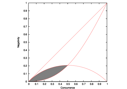
Figure 1: Range of value of negativity for a given concurrence, with its boundaries, as in (54).

The gray field denotes the possible entangled states of the (10)-form on the $\mathcal{C}-\mathcal{N}$ plane. The upper bound of these can be analitically determined, and it can be proven, (see Appendix A) that the following inequality holds for $\mathcal{N}$:

$$\\ \sqrt{(1-\mathcal{C})^{2}+\mathcal{C}^{2}}-(1-\mathcal{C})\leq\mathcal{N}\leq\frac{1}{2}\left(\sqrt{2-(1-2\mathcal{C})^{2}}-1\right)\leq\mathcal{C}$$ (54)

To see, that this upper bound is the tightest, consider the special case, when $\mathbf{w}=\mathbf{z}$. These states realize the boundary, so the second inequality in (54) turns to equality. (In this case $\eta=0$, $r=s$, $\gamma_{+}=2r$, $\gamma_{-}=0$, and for entangled states, $\mathcal{C}=\frac{1}{2}(1-\sqrt{1-4r^{2}})$, $\mathcal{N}=\frac{1}{2}(\sqrt{1+4r^{2}}-1)$. These depend only on $r$, wich can be expressed from $\mathcal{C}$, thus we can express the negativity of these states with their concurrence, and get back the curve of the upper bound.)

It can be seen, by calculating the intersection of the corresponding curves of (54), that for maximally entangled states $\mathcal{C}(\varrho_{max})=\frac{1}{2}$, and $\mathcal{N}(\varrho_{max})=\frac{\sqrt{2}-1}{2}$. We can study the behavior of these states: from the (48) concurrence formula one can see, that

$$\mathcal{C}=\frac{1}{2}\quad\Longleftrightarrow\quad\left(\eta^{2}=0,\quad\text{and}\quad\gamma_{-}^{2}=0,\quad\text{and}\quad\gamma_{+}^{2}=1\right).$$ (55)

The first two of these constraints hold, if and only if $\mathbf{w}^{2}=\mathbf{z}^{2}$, and $r=s$, because of (15), (13) and (46). If $\mathbf{w}^{2}=\mathbf{z}^{2}$ then $r=s$ and $\|\mathbf{w}\|^{2}=\|\mathbf{z}\|^{2}=\frac{1}{2}$ are equivalent, and if $r=s$ then $\gamma_{+}^{2}=4r^{2}=1$, $\|\mathbf{w}\|^{4}-|\mathbf{w}^{2}|^{2}=\frac{1}{4}$ and follows, that $\mathbf{w}^{2}=0$.

$$\mathcal{C}=\mathcal{C}_{max}=\frac{1}{2}\quad\Longleftrightarrow\quad\left(\|\mathbf{w}\|^{2}=\|\mathbf{z}\|^{2}=\frac{1}{2},\quad\text{and}\quad\mathbf{w}^{2}=\mathbf{z}^{2}=0\right).$$ (56)

Since the (34) transformation on $\varrho$ preserves the quantities appearing here, we can easily calculate the (34) canonical form of the maximally entangled state $\varrho^{\prime}$. Let us choose an ansatz of the form (25) and (30) for $\mathbf{w}_{max}^{\prime}$ and $\mathbf{z}_{max}^{\prime}$ as $\mathbf{w}_{max}^{\prime}=\frac{1}{\sqrt{2}}\begin{bmatrix}\cos(\alpha)e^{i\varphi_{1}},\sin(\alpha)e^{i\varphi_{2}},0\end{bmatrix}^{T}$ and $\mathbf{z}_{max}^{\prime}=\frac{1}{\sqrt{2}}\begin{bmatrix}\cos(\beta)e^{i\psi_{1}},\sin(\beta)e^{i\psi_{2}},0\end{bmatrix}^{T}$. These satisfy the first constraint of (56), and from the second follows that $\cos{\alpha}=\sin{\alpha}=\frac{1}{\sqrt{2}}$ and $\varphi_{1}=\varphi_{2}-\frac{\pi}{2}=:\varphi$ and the same for $\mathbf{z}_{max}^{\prime}$.

$$\mathbf{w}_{max}^{\prime}=\frac{1}{2}e^{i\varphi}\begin{bmatrix}1\\ i\\ 0\end{bmatrix},\qquad\mathbf{z}_{max}^{\prime}=\frac{1}{2}e^{i\psi}\begin{bmatrix}1\\ i\\ 0\end{bmatrix}.$$ (57)

Then for the density matrix with maximal concurrence we get the expression

$$\varrho^{\prime}_{max}=\frac{1}{4}\begin{bmatrix}\frac{3}{2}&0&0&0\\ 0&1&e^{i\delta}&0\\ 0&e^{-i\delta}&1&0\\ 0&0&0&\frac{1}{2}\end{bmatrix},$$ (58)

with $\delta=\varphi-\psi$ is the only parameter characterizing this maximally entangled density matrix.

III.4 Purity

The purity is measuring the degree of mixedness of a density matrix. For our $\varrho$ thanks to the special property of $\Lambda$ (see in Eq. (14)) it can easily be calculated. We have the result

$$\operatorname{Tr}\varrho^{2}=\frac{1}{4}(2-\eta^{2}),$$ (59)

$$\frac{1}{4}\leq\operatorname{Tr}\varrho^{2}\leq\frac{1}{2}$$ (60)

by virtue of Eq. (16). The participation ratio is by definition

$$R=\frac{1}{\operatorname{Tr}\varrho^{2}}=\frac{4}{2-\eta^{2}}.$$ (61)

IV Relating different measures of entanglement

Now we would like to discuss the physical meaning of our quantities derived in the previous section. First of all let us notice that the

$${\varrho}_{1}={\rm Tr}_{234}(|\Psi\rangle\langle\Psi|)={\rm Tr_{2}}({\varrho}_{12})={\rm Tr}_{2}(\varrho)=\frac{1}{2}(I+{\bf x}\boldsymbol{\sigma})$$ (62)

$$\varrho_{2}={\rm Tr}_{134}(|\Psi\rangle\langle\Psi|)={\rm Tr_{1}}(\varrho_{12})={\rm Tr}_{1}(\varrho)=\frac{1}{2}(I+{\bf y}\boldsymbol{\sigma})$$ (63)

reduced density matrices describe the entanglement properties of subsystems $1$ and $2$ to the rest of the system described by the four-qubit state $|\Psi\rangle$. It is well-known that the measures describing how much these subsystems are entangled with the rest are ${\cal C}^{2}_{1(234)}=4{\rm Det}(\varrho_{1})$ and ${\cal C}^{2}_{2(134)}=4{\rm Det}(\varrho_{2})$. Due to Eqs. (62-63) these quantities are

$$0\leq{\cal C}^{2}_{1(234)}=1-r^{2}\leq 1,\qquad 0\leq{\cal C}^{2}_{2(134)}=1-s^{2}\leq 1.$$ (64)

Clearly, since ${\varrho}_{1}={\varrho}_{3}$ and ${\varrho}_{2}={\varrho}_{4}$, we also have

$${\cal C}^{2}_{3(124)}={\cal C}^{2}_{1(234)},\qquad{\cal C}^{2}_{4(123)}={\cal C}^{2}_{2(134)}.$$ (65)

Moreover, we already know that ${\varrho}_{12}={\varrho}_{34}={\varrho}$. A straightforward calculation of the two-partite density matrices ${\varrho}_{14}$ and ${\varrho}_{23}$ shows that they again have the form of Eq. (10) with the sign of ${\bf w}$ is changed in the first case and the vectors ${\bf w}$ and ${\bf z}$ are exchanged in the second. Since these transformations do not change the value of the concurrence, we have

$${\cal C}^{2}_{12}={\cal C}^{2}_{14}={\cal C}^{2}_{23}={\cal C}^{2}_{34}.$$ (66)

Now the only two-qubit density matrices we have not discussed yet are the ones ${\varrho}_{13}$ and ${\varrho}_{24}$. Their form is

$$\left({\varrho}_{13}\right)_{iki^{\prime}k^{\prime}}=\frac{1}{2}\left(||{\bf z}||^{2}{\varepsilon}_{ik}{\varepsilon}_{i^{\prime}k^{\prime}}+{\cal B}_{ik}\overline{\cal B}_{i^{\prime}k^{\prime}}\right),\qquad\left({\varrho}_{24}\right)_{jlj^{\prime}l^{\prime}}=\frac{1}{2}\left(||{\bf w}||^{2}{\varepsilon}_{jl}{\varepsilon}_{j^{\prime}l^{\prime}}+{\cal A}_{jl}\overline{\cal A}_{j^{\prime}l^{\prime}}\right).$$ (67)

Recall now the that the (4) transformation property of our four-qubit state gives rise to the corresponding ones for the reduced density matrices

$${\varrho}_{13}\mapsto(U\otimes U){\varrho}_{13}(\overline{U}\otimes\overline{U}),\qquad{\varrho}_{24}\mapsto(V\otimes V){\varrho}_{24}(\overline{V}\otimes\overline{V}).$$ (68)

For $U,V\in SU(2)$ we have $V{\varepsilon}V^{t}=U{\varepsilon}U^{t}={\varepsilon}$, hence the tensors occurring in Eq. (67) transform as

$${\varepsilon}\mapsto{\varepsilon},\qquad{\cal A}\mapsto V{\cal A}V^{t},\qquad{\cal B}\mapsto U{\cal B}U^{t}.$$ (69)

Using the (6) definition of ${\cal A}$ we have for example

$$V{\cal A}V^{t}=\varepsilon\overline{V}{\bf z\overline{\boldsymbol{\sigma}}}V^{t}=\varepsilon\overline{V\overline{\bf z}{\boldsymbol{\sigma}}V^{\dagger}}=\varepsilon\overline{\overline{{\bf z}^{\prime}}{\boldsymbol{\sigma}}}=\varepsilon{\bf z}^{\prime}\overline{\boldsymbol{\sigma}},$$ (70)

where by choosing $V\equiv V_{\bf y}^{\dagger}$ of Eq. (27) we get for ${\bf z}^{\prime}$ the (30) form. Finally these manipulations yield for ${\varrho}_{24}$ the canonical form

$${\varrho}_{24}=\frac{1}{2}\begin{pmatrix}{\kappa}_{0}+{\kappa}_{3}&0&0&{\kappa}_{1}-i{\kappa}_{2}\\ 0&||{\bf w}||^{2}&-||{\bf w}||^{2}&0\\ 0&-||{\bf w}||^{2}&||{\bf w}||^{2}&0\\ {\kappa}_{1}+i{\kappa}_{2}&0&0&\kappa_{0}-\kappa_{3}\end{pmatrix},$$ (71)

where

$$\kappa_{0}=||{\bf z}^{\prime}||^{2}=||{\bf z}||^{2},\quad-\kappa_{1}=|z_{1}^{\prime}|^{2}-|z_{2}^{\prime}|^{2},\quad-\kappa_{2}=2{\rm Re}(z_{1}^{\prime}\overline{z_{2}^{\prime}}),\quad-\kappa_{3}=2{\rm Im}(z_{1}^{\prime}\overline{z_{2}^{\prime}}).$$ (72)

Notice that

$${\kappa}_{0}^{2}={\kappa}_{1}^{2}+{\kappa}_{2}^{2}+{\kappa}_{3}^{2}=||{\bf z}||^{4},$$ (73)

hence the eigenvalues of ${\varrho}_{24}$ are $||{\bf w}||^{2},||{\bf z}||^{2},0,0$, i.e. our mixed state is of rank two. The structure of ${\varrho}_{13}$ is similar with the roles of ${\bf w}$ and ${\bf z}$ exchanged. Following the same steps as in Section III. A. we get for the corresponding squared concurrences the following expressions

$${\cal C}^{2}_{13}=\left(||{\bf z}||^{2}-|{\bf w}^{2}|\right)^{2},\qquad{\cal C}^{2}_{24}=\left(||{\bf w}||^{2}-|{\bf z}^{2}|\right)^{2}.$$ (74)

Let us now understand the meaning of the invariant $\eta$ from the four-qubit point of view. It is known that we have four algebraically independent $SL(2,\mathbf{C})^{\otimes 4}$ invariantsLuque ; Levay denoted by $H,L,M$ and $D$. These are quadratic, quartic, quartic and sextic invariants of the complex amplitudes ${\Psi}_{ijkl}$ respectively. The invariants $H$ and $L$ are given by the expressions

$$H=\Psi_{0}\Psi_{15}-\Psi_{1}\Psi_{14}-\Psi_{2}\Psi_{13}+\Psi_{3}\Psi_{12}-\Psi_{4}\Psi_{11}+\Psi_{5}\Psi_{10}+\Psi_{6}\Psi_{9}-\Psi_{7}\Psi_{8},$$ (75)

and

$$L={\rm Det}\begin{pmatrix}\Psi_{0}&\Psi_{1}&\Psi_{2}&\Psi_{3}\\ \Psi_{4}&\Psi_{5}&\Psi_{6}&\Psi_{7}\\ \Psi_{8}&\Psi_{9}&\Psi_{10}&\Psi_{11}\\ \Psi_{12}&\Psi_{13}&\Psi_{14}&\Psi_{15}\end{pmatrix},$$ (76)

where instead of the binary one we used the decimal labelling. For the explicit form of the remaining two invariants $M$ and $D$ see the paper of Luque and ThibonLuque . A straightforward calculation shows that for our four-qubit state we have $M=D=0$ however,

$$H=-\frac{1}{2}({\bf z}^{2}+{\bf w}^{2}),\qquad L=\frac{1}{16}({\bf z}^{2}-{\bf w}^{2})^{2},$$ (77)

hence

$$|L|=\frac{1}{16}\eta^{2}.$$ (78)

For convenience we also introduce the quantity

$$\sigma\equiv|{\bf w}^{2}+{\bf z}^{2}|=2|H|.$$ (79)

Hence $\eta=|{\bf w}^{2}-{\bf z}^{2}|$ and $\sigma=|{\bf w}^{2}+{\bf z}^{2}|$ are related to the only nonvanishing four qubit invariants $L$ and $H$. Using the definitions of these quantities and Eq. (13) one can check that

$${\cal C}^{2}_{13}=s^{2}+\frac{1}{2}(\eta^{2}+\sigma^{2})-2||{\bf z}^{2}|||{\bf w}^{2}|,\quad{\cal C}^{2}_{24}=r^{2}+\frac{1}{2}(\eta^{2}+\sigma^{2})-2||{\bf w}^{2}|||{\bf z}^{2}|.\quad$$ (80)

Hence we have the inequality

$${\cal C}^{2}_{13}+{\cal C}^{2}_{24}\leq s^{2}+r^{2}+{\eta}^{2}+{\sigma}^{2}.$$ (81)

Moreover, since ${\cal C}^{2}_{12}={\cal C}^{2}_{14}$ after taking the square of Eq.(48) we get

$${\cal C}^{2}_{12}+{\cal C}^{2}_{14}=1-r^{2}-s^{2}-\frac{1}{2}{\eta}^{2}-\sqrt{(1-\eta^{2}-{\gamma}_{-}^{2})(1-\gamma_{+}^{2})}$$ (82)

Combining this result with Eqs.(64) and (80) we obtain

$${\cal C}^{2}_{12}+{\cal C}^{2}_{13}+{\cal C}^{2}_{14}+{\Sigma}_{1}={\cal C}^{2}_{1(234)}\qquad{\cal C}^{2}_{12}+{\cal C}^{2}_{23}+{\cal C}^{2}_{24}+{\Sigma}_{2}={\cal C}^{2}_{2(134)},$$ (83)

where

$${\Sigma}_{1}=2||{\bf z}||^{2}|{\bf w}^{2}|+\sqrt{(\frac{1}{2}\sigma^{2}+p_{+})(\frac{1}{2}\sigma^{2}+p_{-})}-\frac{1}{2}\sigma^{2},$$ (84)

$${\Sigma}_{2}=2||{\bf w}||^{2}|{\bf z}^{2}|+\sqrt{(\frac{1}{2}\sigma^{2}+p_{+})(\frac{1}{2}\sigma^{2}+p_{-})}-\frac{1}{2}\sigma^{2}.$$ (85)

Here

$$p_{\pm}=2||{\bf z}||^{2}||{\bf w}||^{2}\pm\frac{1}{2}(4rs-\eta^{2}).$$ (86)

Notice that by virtue of Eq.(13) $p_{-}$ is nonnegative. Moreover according to Eq. (52), for nonseparable states (${\varrho}_{12},\varrho_{14},\varrho_{34},\varrho_{23}$) we have nonzero negativity hence $4rs>\eta^{2}$ hence $p_{+}$ is also nonnegative. In this case the residual tangles $\Sigma_{1}$ and $\Sigma_{2}$ as defined by Eqs. (84-85) are positive as they should be, hence the generalized Coffman-Kundu-Wootters inequalities of distributed entanglementKundu ; Osborne hold

$${\cal C}^{2}_{12}+{\cal C}^{2}_{13}+{\cal C}^{2}_{14}\leq{\cal C}^{2}_{1(234)}\qquad{\cal C}^{2}_{12}+{\cal C}^{2}_{23}+{\cal C}^{2}_{24}\leq{\cal C}^{2}_{2(134)}.$$ (87)

For separable states we have ${\cal C}_{12}={\cal C}_{14}={\cal C}_{34}={\cal C}_{23}=0$ and a calculation shows that the (87) inequalities in the form ${\cal C}^{2}_{13}\leq{\cal C}^{2}_{1(234)}$ and ${\cal C}^{2}_{24}\leq{\cal C}^{2}_{2(134)}$ still hold with residual tangles

$${\Sigma}_{1}=2||{\bf z}||^{2}(|{\bf w^{2}}|+||{\bf w}||^{2})\qquad{\Sigma}_{2}=2||{\bf w}||^{2}(|{\bf z^{2}}|+||{\bf z}||^{2}).$$ (88)

Eqs. (84), (85) and (88) show the structure of the residual tangle. Unlike in the well-known three-qubit case these quantities among others contain two invariants $\eta$ and $\sigma$ characterizing four-partite correlations. The role of $\sigma$ (which for a general four-qubit state is a permutation-invariant) is to be compared with the similar role the permutation invariant three-tangle ${\tau}_{123}=4|{\cal D}|$ plays (an $SL(2,\mathbf{C})^{\otimes 3}$ invariant) within the three-qubit context. (${\cal D}$ is Cayley’s hyperdeterminantKundu .) An important difference to the three-qubit case is that the residual tangles ${\Sigma}_{1,2}$ seeem to be lacking the important entanglement monotone property. However, according to a conjectureharomkinai the sum ${\Sigma}_{1}+{\Sigma}_{2}$ could be an entanglement monotone. We hope that our explicit form will help to settle this issue at least for our special four-qubit state of Eqs. (1-2).

V Bures metric

As we have emphasized our density matrix ${\varrho}$ can be regarded as a reduced density matrix of a two-particle system on $(\mathbf{C}^{2}\otimes\mathbf{C}^{2})\wedge(\mathbf{C}^{2}\otimes\mathbf{C}^{2})$, meaning

$$\varrho={\Psi}{\Psi}^{\dagger},$$ (89)

where ${\Psi}$ is the $4\times 4$ antisymmetric matrix occurring in Eq. (76). In the space of such fermionic purifications of our density matrix the curve ${\Psi}(t)$ is horizontal, when the differential equation

$$\dot{\Psi}^{\dagger}\Psi=\Psi^{\dagger}\dot{\Psi}$$ (90)

holds. We can satisfy this equation by the ansatz

$$\dot{\Psi}=G\Psi,\qquad G=G^{\dagger}$$ (91)

for some $G=G^{\dagger}$, so that

$$d\varrho=\{G,\varrho\}.$$ (92)

We can define the Bures metric on the space of density matrices, as followsGeom

$$ds^{2}_{B}=\frac{1}{2}\operatorname{Tr}(Gd\varrho).$$ (93)

Let us now take into account the condition ${\Psi}^{T}=-\Psi$. Taking the transpose of Eq. (90), we get

$$\begin{split}\Psi^{T}\dot{\Psi}^{\dagger T}&=\dot{\Psi}^{T}\Psi^{\dagger T},\\ \Psi\dot{\Psi}^{\dagger}&=\dot{\Psi}\Psi^{\dagger}.\end{split}$$ (94)

Using this result, we get a simpler formula for $d\varrho$:

$$d\varrho=\dot{\Psi}\Psi^{\dagger}+\Psi\dot{\Psi}^{\dagger}=2G\Psi\Psi^{\dagger}=2G\varrho.$$ (95)

and to get $G$, we only have to invert $\varrho$. A calculation of the eigenvalues of $\varrho$ shows that they are of the formLNP

$$\lambda_{\pm}=\frac{1}{4}(1\pm\sqrt{1-\eta^{2}}).$$ (96)

Hence ${\varrho}$ is nonsingular iff $\eta\neq 0$ (i.e. iff $|L|\neq 0)$. In the following we consider this case.

For nonsingular density matrices by virtue of Eq. (14), $\varrho^{-1}$ can be calculated easily

$$\varrho^{-1}=\frac{4}{\eta^{2}}\left(\mathbf{1}-\Lambda\right),$$ (97)

hence:

$$G=\frac{1}{2}d\varrho\varrho^{-1}=\frac{1}{2\eta^{2}}\left(d\Lambda-d\Lambda\Lambda\right),$$ (98)

and the Bures-metric:

$$ds^{2}_{B}=\frac{1}{4\eta^{2}}\operatorname{Tr}\left(d\Lambda d\Lambda-d\Lambda\Lambda d\Lambda\right).$$ (99)

Since $\Lambda$ is idempotent and traceless, one can see, that the trace of the second term equals to zero: $2\operatorname{Tr}(d\Lambda\Lambda d\Lambda)=\operatorname{Tr}(d\Lambda d(\Lambda^{2}))=\operatorname{Tr}(d\Lambda d(-\eta^{2})\mathbf{1})=0$. Let us introduce the quantities $f_{ij}=w_{i}\overline{z}_{j}+\overline{w}_{i}z_{j}$. With this notation we have

$$ds^{2}_{B}=\frac{1}{\eta^{2}}\left(dx_{i}dx_{i}+dy_{j}dy_{j}+df_{ij}df_{ij}\right),$$ (100)

(summation on $i,j=1,2,3$ is implied.) Moreover, a calculation shows that $\eta^{2}=1-(x_{i}x_{i}+y_{j}y_{j}+f_{ij}f_{ij})$, so after putting the quantities $x_{i}$, $y_{j}$, $f_{ij}$ into a $15$ component vector $\mathbf{k}\in\mathbf{R}^{15}$ our final result is the nice formula

$$ds^{2}_{B}=\frac{1}{1-\mathbf{k}^{2}}d\mathbf{k}^{2}=\frac{1}{4}\eta^{2}\left[\frac{4d\mathbf{k}^{2}}{(1-\mathbf{k}^{2})^{2}}\right].$$ (101)

Let us compare this formula with the one obtained for the Bures metric of one-qubit density matrices arising as a reduced density matrix from a pair of distinguishable qubitsLevay2

$$dl^{2}_{B}=\frac{1}{4\cosh^{2}\beta}\left(d\beta^{2}+\sinh^{2}\beta d{\Omega}^{2}\right),$$ (102)

where $1-C^{2}=\tanh^{2}\beta$ with $C$ is the pure state concurrence for two qubits, and $d\Omega^{2}$ is the usual line element on the two-sphere $S^{2}$ expressed by the angular coordinates $\vartheta$ and $\varphi$. Since the space of one-qubit density matrices is the Bloch-ball ${\bf B}^{3}$ this parametrization provides a map between the upper sheet of the double sheeted hyperboloid ${\bf H}^{3}$ and ${\bf B}^{3}$. The standard metric on ${\bf H}^{3}$ is just $d{\beta}^{2}+\sinh^{2}\beta d{\Omega}^{2}$. Hence we see that the Bures metric is up to the conformal factor $C^{2}/4$ is just the standard metric on the upper sheet of the double sheeted hyperboloid $H^{3}$. However, using the stereographic projection one can show that

$$d{\beta}^{2}+\sinh^{2}\beta d{\Omega}^{2}=\frac{4{\bf dR}^{2}}{(1-{\bf R}^{2})^{2}},$$ (103)

where $R_{1}R_{2}$ and $R_{3}$ can alternatively be used to parametrize ${\bf B}^{3}$. Hence we can write

$$dl^{2}_{B}=\frac{1}{4}C^{2}\left[\frac{4{\bf dR}^{2}}{(1-{\bf R}^{2})^{2}}\right]$$ (104)

where the metric on the right is the standard Poincaré metric on the unit ball which is now just the Bloch-ball. Comparing this equation with our previous expression of Eq. (101) we see that it is up to the conformal factor $\eta^{2}/4$ is just the Poincaré metric on the Poincaré ball ${\bf B}^{15}$. We emphasize however, that unlike the usual one-qubit mixed state where all the Bloch parameters characterizing the density matrix are independent, here the $15$ parameters associated to the vector ${\bf k}$ are subject to nontrivial constraints. These constraints describe some nontrivial embedding of the space of nonsingular density matrices ${\cal D}$ into the Bloch ball ${\bf B}^{15}$ with our Bures metric of Eq. (101).

VI Conclusions

In this paper we investigated the structure of a $12$ parameter family of two-qubit density matrices with fermionic purifications. Our starting point was a four-qubit state with a special antisymmetry constraint imposed on its amplitudes. Such states are elements of the space $(\mathbf{C}^{2}\otimes\mathbf{C}^{2})\wedge(\mathbf{C}^{2}\otimes\mathbf{C}^{2})$ and the admissible local operations are of the form $(U\otimes V)\otimes(U\otimes V)\in SL(2,\mathbf{C})^{\otimes 4}$. Our density matrices are arising as the reduced ones ${\varrho}={\varrho}_{12}={\rm Tr}_{34}(|\Psi\rangle\langle\Psi|)$. Since the $12$ subsystem is indistinguishable from the $34$ one we have ${\varrho}_{12}={\varrho}_{34}$. We obtained an explicit form for ${\varrho}$ in terms of the $6$ independent complex amplitudes ${\bf w}$ and ${\bf z}$ of our four-qubit states. Employing local unitary transformations of the form $U\otimes V\in SU(2)\times SU(2)\subset SL(2,\mathbf{C})\times SL(2,\mathbf{C})$ we derived the canonical form for ${\varrho}$. This form enabled an explicit calculation for different entanglement measures. We have calculated the Wootters concurrence, the negativity, and the purity. The quantities occurring in these formulae (and some additional ones) are subject to monogamy relations of distributed entanglement similar to the ones showing up in the Coffman-Kundu-Wootters relations for three-qubits. They are characterizing the entanglement trade off between different subsystems. We have entanglement measures $\eta$ and $\sigma$ describing the intrinsically four-partite correlations, quantities ( Wootters concurrences) keeping track the mixed state entanglement of the bipartite subsystems embedded in the four-qubit one. Finally we have the independent quantities ${\cal C}^{2}_{1(234)}$ and ${\cal C}^{2}_{2(134)}$ measuring how much subsystems $1$ and $2$ are entangled individually to the rest. We derived explicit formulas displaying how these important quantities are related. At last we have studied in some detail the Bures geometry underlying the structure of these density matrices. We have shown that the constraint of antisymmetry makes it possible to obtain a nice explicit formula for the Bures metric reminiscent of the ones known from hyperbolic geometryUngar .

VII Acknowledgment

One of us (P. L.) would like to express his gratitude to Professor Werner Scheid for his warm hospitality at the Department of Theoretical Physics of the Justus Liebig University of Giessen where part of this work was completed. Financial support from the Országos Tudományos Kutatási Alap (OTKA) (Grants No. T046868, T047041, and T038191) is gratefully acknowledged.

Appendix A Upper bound of negativity

In this fermionic-correlated case, defined by equations (10), (11), (12) and (15), we can prove the following inequality:

Theorem: For all entangled $\varrho$:

$$\mathcal{N}(\varrho)\leq\frac{1}{2}\left(\sqrt{2-(1-2\mathcal{C}(\varrho))^{2}}-1\right).$$ (105)

Proof: Insert Eqs. (48) and (52) into (105):

$$\frac{1}{2}\left(\sqrt{1-\eta^{2}+4rs}-1\right)\leq\frac{1}{2}\left(\sqrt{2-\left(1-\sqrt{1-\gamma_{-}^{2}-\eta^{2}}+\sqrt{1-\gamma_{+}^{2}}\right)^{2}}-1\right),$$ (106)

after some algebra, we can rearrange the terms:

$$\begin{split}0&\leq 2\eta^{2}-2+\gamma_{-}^{2}+\gamma_{+}^{2}-4rs\\ &\qquad+2\sqrt{1-\gamma_{-}^{2}-\eta^{2}}-2\sqrt{1-\gamma_{+}^{2}}+2\sqrt{1-\gamma_{-}^{2}-\eta^{2}}\sqrt{1-\gamma_{+}^{2}},\end{split}$$ (107)

If follows from the definition (46) that $\gamma_{+}^{2}-4rs=\gamma_{-}^{2}$. With this:

$$0\leq-(1-\gamma_{-}^{2}-\eta^{2})+\sqrt{1-\gamma_{-}^{2}-\eta^{2}}-\sqrt{1-\gamma_{+}^{2}}+\sqrt{1-\gamma_{-}^{2}-\eta^{2}}\sqrt{1-\gamma_{+}^{2}}.$$ (108)

The right-hand side is factorizable:

$$0\leq\left(\sqrt{1-\gamma_{-}^{2}-\eta^{2}}-\sqrt{1-\gamma_{+}^{2}}\right)\left(1-\sqrt{1-\gamma_{-}^{2}-\eta^{2}}\right).$$ (109)

The second parenthesis is obviously positive. For entangled states $\mathcal{C}(\varrho)>0$, and the first parenthesis is proportional to the concurrence, which is strictly positive. Q.E.D.

References

• (1) M. A. Nielsen and I. L. Chuang, Quantum Computation and Quantum Information, Cambridge University Press, Cambridge, England, 2000.
• (2) Ingemar Bengtsson, Karol Życzkowski, Geometry of Quantum States, Cambridge University Press, 2006.
• (3) M. Ohya and D. Petz, Quantum entropy and its use, Springer Verlag, Berlin, 1993.
• (4) W. K. Wootters, Phys. Rev. Lett. 80, 2245 (1998), S. Hill and W. K. Wootters, Phys. Rev. Lett. 78, 5022 (1997).
• (5) For a nice summary see the relevant chapter of Ref.2
• (6) A. Uhlmann, Phys. Rev. A63 032307 (2000).
• (7) A. Osterloh and J. Siewert, Phys. Rev. A72, 012337 (2005).
• (8) C. M. Caves, C. A. Fuchs and P. Rungta, Found. Phys. Lett. 14, 199 (2001).
• (9) F. Verstraete, K. Audenaert, J. Dehaene, B. De Moor, J. Phys. A34, 10327 (2001). K. Audenaert, F. Verstraete, T. De Bie, B. De Moor, arXiv:quant-ph/0012074.
• (10) S. Ishizaka and T. Hiroshima, Phys. Rev. A62, 022310 (2000).
• (11) J. Eisert and M. B. Plenio, J. Mod. Opt. 46, 145 (1999).
• (12) V. Coffman, J. Kundu and W. K. Wootters, Phys. Rev. A61, 052306 (2000).
• (13) P. Zanardi, D. Lidar and S. Lloyd, Phys. Rev. Lett. 92, 060402 (2004).
• (14) T. Osborne, F. Verstraete, Phys. Rev. Lett. 96, 220503 (2006).
• (15) J. Schliemann, J. I. Cirac, M. Kus, M. Lewenstein and D. Loss, Phys. Rev. A64, 022303 (2001).
• (16) P. Lévay, Sz. Nagy, J. Pipek, Phys. Rev. A72, 022302 (2005).
• (17) J-G. Luque and J-Y. Thibon, Phys. Rev. A67 042303 (2003).
• (18) A. Peres, Phys. Rev. Lett. 77, 1413 (1996).
• (19) P. Lévay, J. Phys. A39, 9533 (2006).
• (20) P. Lévay, J. Phys. A37, 1821 (2004).
• (21) Y-K Bai, D. Yang, Z. D. Wang, Phys. Rev. A76, 022336 (2007).
• (22) J. Chen, L. Fu, A. A. Ungar and X. Zhao, Phys. Rev. A65 024303 (2002).