Magnesium doped helium nanodroplets

Abstract

We have studied the structure of ⁴He droplets doped with magnesium atoms using density functional theory. We have found that the solvation properties of this system strongly depend on the size of the ⁴He droplet. For small drops, Mg resides in a deep surface state, whereas for large size drops it is fully solvated but radially delocalized in their interior. We have studied the $3s3p$ ¹P${}_{1}\leftarrow 3s^{2}$ ¹S₀ transition of the dopant, and have compared our results with experimental data from laser induced fluorescence (LIF). Line broadening effects due to the coupling of dynamical deformations of the surrounding helium with the dipole excitation of the impurity are explicitly taken into account. We show that the Mg radial delocalization inside large droplets may help reconcile the apparently contradictory solvation properties of magnesium as provided by LIF and electron-impact ionization experiments. The structure of ⁴He drops doped with two magnesium atoms is also studied and used to interpret the results of resonant two-photon-ionization (R2PI) and LIF experiments. We have found that the two solvated Mg atoms do not easily merge into a dimer, but rather form a weakly-bound state due to the presence of an energy barrier caused by the helium environment that keep them some $9.5$ Å apart, preventing the formation of the Mg₂ molecule. From this observation, we suggest that Mg atoms in ⁴He drops may form, under suitable conditions, a soft “foam”-like aggregate rather than coalesce into a compact metallic cluster. Our findings are in qualitative agreement with recent R2PI experimental evidences. We predict that, contrarily, Mg atoms adsorbed in ³He droplets do not form such metastable aggregates.

I Introduction

Optical investigations of atomic impurities in superfluid helium nanodroplets have drawn considerable attention in recent years,Sti01 ; Sti06 as the shifts of the electronic transition lines (atomic shifts) are a very useful observable to determine the location of the foreign atom attached to a helium drop.Bar06 In this context, the study of magnesium atoms attached to helium drops has unraveled an interesting and somewhat unexpected solvation behaviour as a function of the number ($N$) of helium atoms in the drop. Diffusion Monte Carlo (DMC) calculationsMel05 carried out for small drops containing a number of helium atoms up to $N=50$ indicate that a Mg atom is not fully solvated in drops of sizes below $N\sim 30$. More recent quantum Monte Carlo calculations Elh07 ; Elh08 suggest a surface Mg state for ⁴He clusters with up to $\sim 200$ atoms. Density Functional Theory (DFT) calculationsHer07 for ³He_N and ⁴He_N nanodroplets with $N\geq 300$ doped with alkaline earth atoms have shown that Mg atoms are solvated in their interior, in agreement with the analysis of Laser Induced Flourescence (LIF)Reh00 and Resonant Two-Photon-Ionization (R2PI) experiments.Prz07 LIF experiments on the absorption and emission spectra of Mg atoms in liquid ³He and ⁴He have been reported and successfully analyzed within a vibrating atomic bubble model, where full solvation of the impurity atom is assumed.Mor99 ; Mor06 A more recent experimentRen07 in which electron-impact ionization data from Mg doped ⁴He drops with about 10⁴ atoms seems to indicate that magnesium is instead at the surface of the droplet, in disagreement with the above mentioned LIF and R2PI experiments.

There is some ambiguity associated with the notion of solvation in a helium droplet. For not too small droplets, one may consider that Mg is fully solvated when its position inside the droplet is such that its solvation energy or atomic shift do not appreciably differ from their asymptotic values in bulk liquid helium, as both quantities approach such limit fairly alongside. However, for very small drops the energy or atomic shifts of an impurity atom at the center of the drop may still differ appreciably from the bulk liquid values because there is not enough helium to saturate these quantities. This is the case, e.g., of Mg@⁴He₅₀ studied in Ref. Mel05, .

Mella et al.Mel05 have discussed how the solvation properties of magnesium are affected by the number of helium atoms in small ⁴He drops. Since DMC calculations cannot be extended to the very large drops involved in LIF experiments,Reh00 they could not carry out a detailed comparison between their calculated atomic shifts and the experiments. They also pointed out the sensitivity of the Mg solvation properties on apparently small differences in the He-Mg pair potentials available in the literature.

The aim of the present work is to re-examine the solvation of magnesium in ⁴He nanodroplets from the DFT perspective, extending our previous calculationsHer07 down to drops with $N\sim 50$ atoms and improving the DFT approach (i) by treating the dopant as a quantal particle instead of as an external field, and (ii) by fully taking into account the coupling of the dipole excitation of the impurity with the dynamical deformations of the helium around the Mg atom. Our results confirm that full solvation of a Mg atom in ⁴He drops requires a minimum number of helium atoms, and disclose some unusual results for small drops. We calculate the absorption spectrum of a Mg atom attached to small and large drops, finding a good agreement with the experiments for the latter. We discuss in a qualitative way the effect of the impurity angular momentum on the electron-impact ionization yield and on the absorption spectrum. We also address the structure of a two-magnesium doped drop; the results are used to discuss the scenario proposed by Meiwes-Broer and collaborators to interpret their experimental results on R2PI.Prz07

This work is organized as follows. In Sec. II we briefly present our density functional approach, as well as results for the structure of Mg@⁴He_N drops. The method we have employed to obtain the atomic shifts is discussed in Sec. III, and applied to the case of Mg-doped ⁴He droplets in Sec. IV. In Sec. V we study how the presence of a second magnesium atom in the droplet may alter both the helium drop structure and the calculated atomic shift. A summary is presented in Sec. VI, and some technical details of our calculations are described in the appendices.

II DFT description of helium nanodroplets

II.1 Theoretical approach

In recent years, static and time-dependent density functional methodsDal95 ; Gia03 ; Leh04 have become increasingly popular to study inhomogeneous liquid helium systems because they provide an excellent compromise between accuracy and computational effort, allowing to address problems inaccessible to more fundamental approaches. Although DFT cannot take into account the atomic, discrete nature of these systems, it can nevertheless address highly inhomogenous helium systems at the nanoscale,Anc05 including the anisotropic deformations induced by atomic dopants in helium drops (see Ref. Bar06, for a recent overview on the physics of helium nanodroplets).

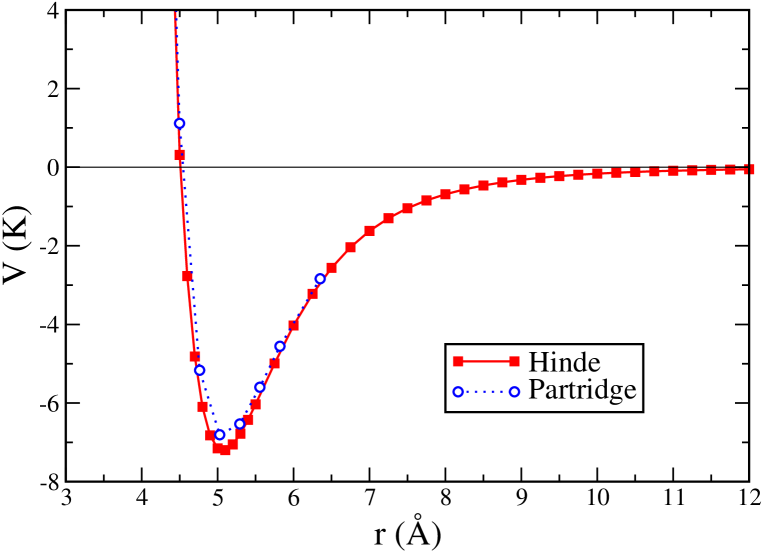
Figure 1: (Color online) $X^{1}\Sigma$ Mg-He pair potentials used in this work: squares connected with a solid line, from Ref. Hin03, ; circles connected with a dotted line, from Ref. Par01, .

Our starting point is the Orsay-Trento density functional,Dal95 together with the Mg-He adiabatic ground-state potential $X^{1}\Sigma$ of Ref. Hin03, , here denoted as $V_{Mg-He}$. To check the sensitivity of our results to the details of different available pair potential describing the Mg-He interaction, we also use the sligthly less attractive potential computed in Ref. Par01, . For the sake of comparison, we plot both potentials in Fig. 1. Despite the apparently minor differences between these two potential curves, they cause very different solvation properties of Mg in small ⁴He drops, as we will show in the following.

The energy of the Mg-helium system is written as a functional of the Mg wave function $\Phi(\mathbf{r})$ and the ⁴He “order parameter” $\Psi(\mathbf{r})=\sqrt{\rho(\mathbf{r})}$, where $\rho(\mathbf{r})$ is the ⁴He atomic density:

$$E[\Psi,\Phi] = \frac{\hbar^{2}}{2\,m_{He}}\int\mathrm{d}^{3}\mathbf{r}\,|\nabla\Psi(\mathbf{r}\,)|^{2}+\int\mathrm{d}^{3}\mathbf{r}\,{\cal E}(\rho)$$ (1)

$$+ \frac{\hbar^{2}}{2\,m_{Mg}}\int\mathrm{d}^{3}\mathbf{r}\,|\nabla\Phi(\mathbf{r}\,)|^{2}+\int\int\mathrm{d}^{3}\mathbf{r}\,\mathrm{d}^{3}\mathbf{r^{\prime}}\,|\Phi(\mathbf{r})|^{2}\,V_{Mg-He}(|\mathbf{r}-\mathbf{r^{\prime}}|)\,\rho(\mathbf{r^{\prime}})\;.$$

In this expression, ${\cal E}(\rho)$ is the ⁴He “potential energy density”.Dal95 Minimizing $E$ under the constraints of a given $N$ and a normalized Mg wave function, yields the ground state of the drop-impurity complex. To address the solvation of the Mg atom, we have found it convenient to minimize $E$ subjected to the additional constraint of a fixed distance ${\cal Z}_{0}$ between the centers of mass of the helium moiety and of the impurity atom which, due to the symmetry of the problem, can both be taken on the $z$ axis. This is done following a method -borrowed from Nuclear Physics- similar to that used to describe the fission of rotating ³He drops.Gui93 Specifically, we minimize the expression

$$E+\frac{\lambda_{C}}{2}[{\cal Z}-{\cal Z}_{0}]^{2}\;,$$ (2)

where ${\cal Z}$ is the average distance between the impurity and the center of mass of the helium droplet

$${\cal Z}=\int d\mathbf{r}^{3}\,z\,|\Phi(\mathbf{r})|^{2}-\frac{1}{N}\int d\mathbf{r}^{3}\,z\,\rho(\mathbf{r})\;.$$ (3)

$\lambda_{C}$ is an arbitrary constant. The value $\lambda_{C}\sim$ 1000 K Å^-2 has been used in our calculations, which ensures that the desired ${\cal Z}_{0}$ value is obtained within a 0.1 % accuracy.

We have solved the Euler-Lagrange equations which result from the variations with respect to $\Psi^{*}$ and $\Phi^{*}$ of the constrained energy Eq. (2), namely

$$-\frac{\hbar^{2}}{2\,m_{He}}\Delta\Psi+\left\{\frac{\delta{\cal E}}{\delta\rho}+U_{He}-\lambda_{C}({\cal Z}-{\cal Z}_{0})\frac{z}{N}\right\}\Psi=\mu\Psi$$ (4)

$$-\frac{\hbar^{2}}{2\,m_{Mg}}\Delta\Phi+\left\{U_{Mg}+\lambda_{C}({\cal Z}-{\cal Z}_{0})\,z\right\}\Phi=\varepsilon\Phi\;,$$ (5)

where $\mu$ is the helium chemical potential and $\varepsilon$ is the lowest eigenvalue of the Schrödinger equation obeyed by the Mg atom. The above coupled equations have to be solved selfconsistently, starting from an arbitrary but reasonable choice of the unknown functions $\Psi$ and $\Phi$. The fields $U_{He}$ and $U_{Mg}$ are defined as

$$U_{He}(\mathbf{r}) = \int\mathrm{d}^{3}\mathbf{r^{\prime}}\,|\Phi(\mathbf{r^{\prime}})|^{2}\,V_{Mg-He}(|\mathbf{r}-\mathbf{r^{\prime}}|)$$

$$U_{Mg}(\mathbf{r}) = \int\mathrm{d}^{3}\mathbf{r^{\prime}}\,\rho(\mathbf{r^{\prime}})\,V_{Mg-He}(|\mathbf{r}-\mathbf{r^{\prime}}|)\;.$$ (6)

In spite of the axial symmetry of the problem, we have solved the above equations in three-dimensional (3D) cartesian coordinates. The main reason is that these coordinates allow to use fast Fourier transformation techniquesFFT to efficiently compute the convolution integrals entering the definition of ${\cal E}(\rho)$, i.e. the mean field helium potential and the coarse-grained density needed to compute the correlation term in the He density functional, Dal95 as well as the fields defined in Eq. (6).

The differential operators in Eqs. (1,4,5) have been discretized using 13-point formulas for the derivatives. Eqs. (4-5) have been solved employing an imaginary time method;Pre92 some technical details of our procedure are given in Ref. Anc03, . Typical calculations have been performed using a spatial mesh step of 0.5 Å. We have checked the stability of the solutions against reasonable changes in the spatial mesh step.

II.2 Structure and energetics of Mg-doped helium nanodroplets

Equations (4-5) have been solved for $\lambda_{C}=0$ and several $N$ values, namely $N=30$, 50, 100, 200, 300, 500, 1000, and 2000. This yields the ground state of the drop-impurity complex, and will allow us to study the atomic shift for selected cluster sizes.

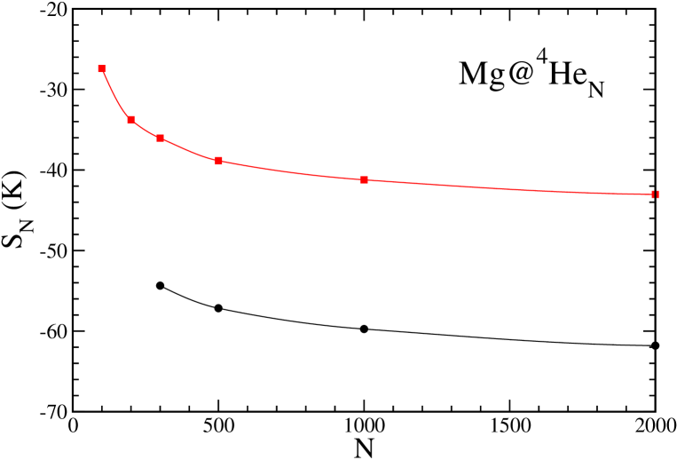
Figure 2: Energy of the Mg atom as a function of the number of atoms in the drop, obtained using the Mg-He potential of Ref. Hin03, (squares). The values given in Ref. Her07, are also displayed (dots). The lines are drawn to guide the eye.

Figure 2 shows the energy of a magnesium atom in a drop, defined as the energy difference

$$S_{N}(Mg)=E(Mg@^{4}He_{N})-E(^{4}He_{N})\;.$$ (7)

We compare in Fig. 2 the $S_{N}(Mg)$ values here obtained with those of Ref. Her07, , where the Mg atom was treated as an infinitely massive particle -i.e., as a fixed external field acting on the ⁴He drop. The neglect of the quantum kinetic energy of the impurity overestimates the impurity solvation energies by quite a large amount, about 19.7 K for $N=50$ and 18.8 K for $N=2000$. The value we have found for $S_{50}(Mg)$, $-18.4$ K, compares well with the DMC result of Ref. Elh08, ($-21$ K), showing that DFT performs quite well for small clusters,Bar06 far from the regime for which it was parametrized. The DMC energy found for the same system is $\sim-168.2$ K,Mel05 whereas our DFT result is $\sim-157.0$ K, and the “asymptotic” DMC value for $S_{200}(Mg)$, $-33.1$ K, compares well with the DFT value, still far from the limit value corresponding to a very large helium drop (see Fig. 2).

The solvation properties of the Mg atom are determined by a delicate balance between the different energy terms –surface, bulk and helium-impurity– in Eq. (1), whose contribution is hard to disentangle and depends on the number of atoms in the drop, as shown by DMC and DFT calculations. To gain more insight into the solvation process of magnesium in small ⁴He droplets, we have computed the energy of the doped droplet as a function of the impurity position ${\cal Z}_{0}$.

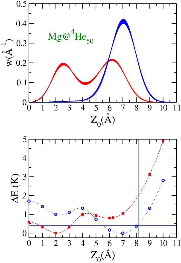
Figure 3: (Color online) Bottom panel: total energy (K) of Mg@⁴He₅₀ as a function of ${\cal Z}_{0}$ (Å) obtained using the Mg-He potential of Ref. Hin03, (squares) and of Ref. Par01, (circles). The energies are referred to their equilibrium values, -157.0 K and -153.8 K, respectively. The vertical line locates the drop surface at $R_{1/2}=r_{0}N^{1/3}$, with $r_{0}=2.22$ Å. The horizontal line has been drawn 0.4 K above the equilibrium energy. Top panel: probability densities for the configurations displayed in the bottom panel; the single peak distribution corresponds to the Mg-He interaction of Ref. Par01, .

The bottom panel in Fig. 3 shows $E({\cal Z}_{0})$ for $N=50$, as computed using the two different Mg-He pair interactions shown in Fig. 1 (the discussion of the top panel is postponed until Sec. IV.A). It can be seen that $E({\cal Z}_{0})$ in both cases displays two local minima. In one case (i.e. for the sligtly less attractive potential in Fig. 1) a “surface” state for the Mg atom is energetically preferred, while in the other case the impurity prefers to sit in the interior to the droplet (although not exactly at its center). These results are in agreement with the DMC calculations of Ref. Mel05, , where it has been shown that a bimodal distributions for the Mg radial probability density function with respect to the center-of-mass of the helium moiety appears for $N\leq 30$.Mel05 More recent DMC calculations carried out up to $N\sim 200$ dropsElh08 seem to point out that Mg is always in a surface state, although somewhat beneath the drop surface. Our DFT calculations yield that Mg is already solvated for $N=200$.

For both pair potentials, the bottom panel of Fig. 3 shows that the two local minima in $E({\cal Z}_{0})$ are separated by an energy barrier of about 1 K height, allowing the impurity to temporarily visit, even at the experimental temperature $T\sim 0.4$ K, the less energetically favored site. This causes changes in the total energy of the system by less that 1 %, but has a large effect on the value of the atomic shift. We will address this important issue, and its consequencies on the computed spectral properties of Mg@He_N in the next Sections.

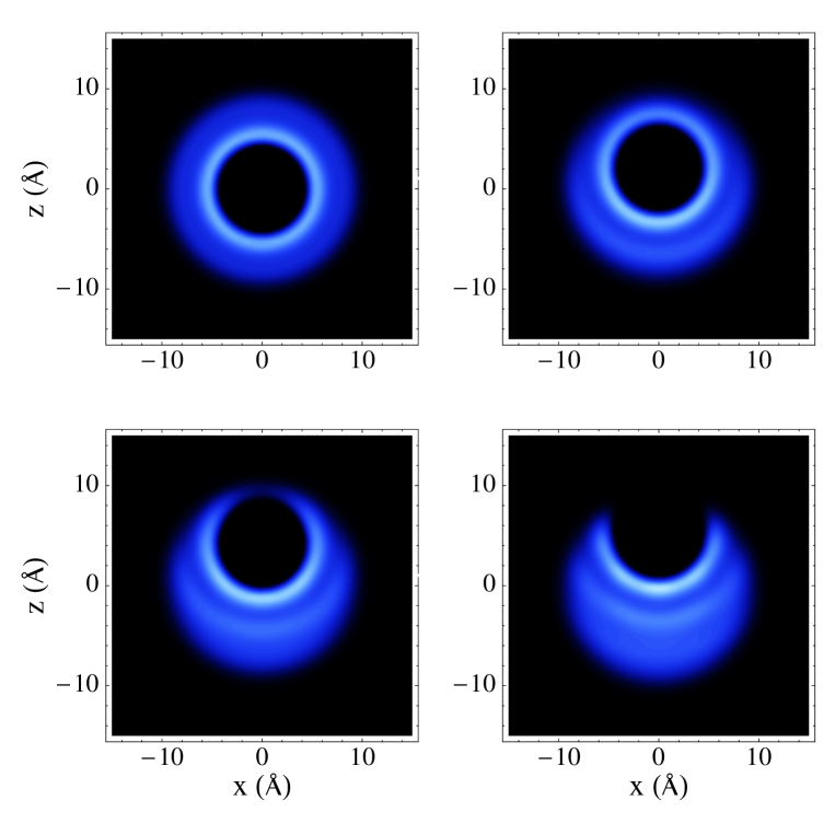
Figure 4: (Color online) Helium density plots of the Mg@⁴He₅₀ droplet in the $y=0$ plane obtained using the Mg-He potential of Ref. Hin03, . From top to bottom and left to right, the ${\cal Z}_{0}$ values correspond to the stationary points displayed in Fig. 3, namely 0, 2, 4, and 6 Å, respectively. The brighter regions are the higher density ones.

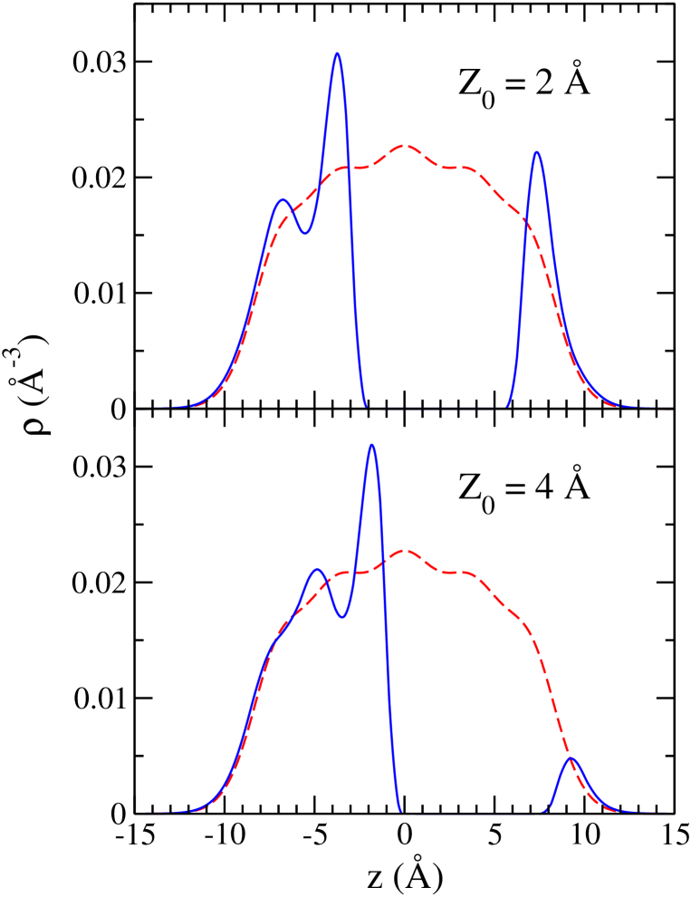
Figure 5: (Color online) Helium density profiles of the Mg@⁴He₅₀ droplet along the $z$ axis obtained using the Mg-He potential of Ref. Hin03, . The ${\cal Z}_{0}$ value is indicated in each panel. Dashed lines, pure drops; solid lines, doped drops.

Figure 4 shows the helium configurations for the four stationary points displayed in Fig. 3, namely those corresponding to ${\cal Z}_{0}=0$, 2, 4, and 6 Å. Although the preference for the surface or the solvated state depends on the He-Mg pair potential used in the calculations, similarly to the case of other alkali atoms,Her07 this does not seem to be the case for the stationary points at ${\cal Z}_{0}=2$ and 4 Å that are present in both curves. We have compared in Fig. 5 the density profiles along the $z$ axis for the ${\cal Z}_{0}=2(4)$ Å configuration with the profile of the pure ⁴He drop, finding that the appearence of these stationary points is related to the position of the density peak in the first helium solvation shell with respect to a maximum(minimum) of the density of the pure drop. We see that a minimum(maximum) in the energy is associated with a constructive(destructive) interference in the oscillation pattern of the He density. We are lead to conclude that the interplay between the density oscillations already present in pure drops, and the solvation shells generated by the impurity plays an important role in the solvation properties of the Mg atom. This effect is also present, although to a lesser extent, in Ca-doped ⁴He nanodroplets.Her08

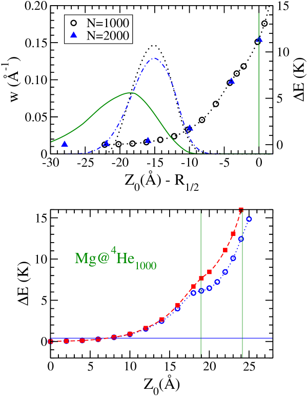
Figure 6: (Color online) Bottom panel: total energy (K) of Mg@⁴He₁₀₀₀ as a function of ${\cal Z}_{0}$ (Å) obtained using the Mg-He potential of Ref. Hin03, (squares) and of Ref. Par01, (circles). The energies are referred to their equilibrium values, -5482.0 K and -5476.8 K, respectively. The vertical lines roughly delimit the drop surface region, conventionally defined as the radial distance between the points where the density equals 0.1$\rho_{b}$ and 0.9$\rho_{b}$, being $\rho_{b}=0.0218$ Å^-3 the bulk liquid density. The horizontal line has been drawn 0.4 K above the equilibrium energy. Top panel: total energy (K) of Mg@⁴He_N with $N=1000$ and 2000 (vertical right scale) as a function of ${\cal Z}_{0}$ (Å) obtained using the Mg-He potential of Ref. Hin03, . The energies are referred to their equilibrium values, $-5482.0$ K and $-11\,629.8$ K, respectively, and the distances (horizontal scale) are referred to the $R_{1/2}$ radius; also shown are the corresponding probability densities (vertical left scale): dot(dot-dash) line, $N=1000(2000)$. The solid line represents the probability density of the $N=10\,000$ drop.

Eventually, for larger drops Mg becomes fully solvated. We have found that this is the case whichever of these two potentials we use (see for instance the bottom panel of Fig. 6). For this reason, the results we discuss in the following have been obtained with the Mg-He pair potential of Ref. Hin03, , unless differently stated.

When the Mg atom is fully solvated, e.g. for $N=1000$, we have found that $E({\cal Z}_{0})$ grows monotonously as ${\cal Z}_{0}$ increases (i.e. as the Mg atom approaches the droplet surface). This is shown in the bottom panel of Fig. 6. To better understand how $E({\cal Z}_{0})$ depends on $N$, we have plotted in the top panel of Fig. 6 the energy of the $N=1000$ and 2000 doped drops, referred to their equilibrium value, as a function of the distance from the dividing surface, i.e. the radius $R_{1/2}$ at which the density of the pure drop equals $\rho_{b}/2$, $\rho_{b}$ being the liquid density value ($R_{1/2}=r_{0}N^{1/3}$, with $r_{0}=$ 2.22 Å). These radii are 22.2 and 28.0 Å for $N=1000$ and 2000, respectively.

The top panel of Fig. 6 shows that most of the change in $\Delta E$ takes place in the 15 Å outer region of the drop, irrespective of its size. As a consequence of the flatness of $E({\cal Z}_{0})$, the magnesium atom is very delocalized in the radial direction even in relatively small drops. This delocalization might affect the absorption spectrum of the attached Mg atom, and also must be explicitly considered in the interpretation of the electron-impact yield experiments.Ren07 We address this issue in Sec. IV.

III Excitation spectrum of a Mg atom attached to a ⁴He drop

Lax methodLax52 offers a realistic way to study the absorption spectrum of a foreign atom embedded in liquid drops. It makes use of the Franck-Condon principle within a semiclassical approach, and it has been widely employed to study the absorption spectrum of atomic dopants attached to ⁴He drops, see e.g. Ref. Her08, and references therein. The method is usually applied in conjunction with the diatomics-in-molecules theory,Ell63 which means that the atom-drop complex is treated as a diatomic molecule, where the helium moiety plays a role of the other atom.

In the original formalism, to obtain the line shape one has to carry out an average on the possible initial states of the system that may be thermally populated. Usually, this average is not needed for helium drops, as their temperature, about $0.4$ K,Toe04 is much smaller than the vibrational excitation energies of the Mg atom in the mean field represented by the second of Eqs. (6). In small helium droplets thermal effects can show up in the Mg absorption spectrum due to the high mobility of the atom. For large drops, thermal motion plays a minor role, as the Mg atom hardly gets close enough to the drop surface to have some effect on the line shape. In this case, however, dynamical deformations of the cavity around the impurity may be relevant.Ler93 ; Kin96

The line shape for electronic transitions from the ground state $(gs)$ to the excited state $(ex)$ in a condensed phase system can be written as

$$I(\omega)\propto\int\mathrm{d}t~{}\mathrm{e}^{-i\omega t}\langle\Psi^{gs}|D_{ge}^{\dagger}~{}\mathrm{e}^{\frac{it}{\hbar}\mathcal{H}_{ex}}~{}D_{ge}~{}\mathrm{e}^{-\frac{it}{\hbar}\mathcal{H}_{gs}}|\Psi^{gs}\rangle\;,$$ (8)

where $D_{\mathrm{ge}}$ is the matrix element of the electric dipole operator, $|\Psi^{gs}\rangle$ is the ground state of the system, and $\mathcal{H}_{gs}$ and $\mathcal{H}_{ex}$ are the Hamiltonians that describe the ground and excited states of the system respectively.

$I(\omega)$ is evaluated using the Born-Oppenheimer approximation and the Franck-Condon principle, whereby the heavy nuclei do not change their positions or momenta during the electronic transition. If the excited electron belongs to the impurity, the helium cluster remains frozen, so that the relevant coordinate is the relative position $\mathbf{r}$ between the cluster and the impurity. This principle amounts to assuming that $D_{\mathrm{ge}}$ is independent of the nuclear coordinates. Taking into account that $\mathrm{e}^{-\frac{it}{\hbar}\mathcal{H}_{gs}}|\Psi^{gs}\rangle=\mathrm{e}^{-it\omega_{gs}}|\Psi^{gs}\rangle$ and projecting on eigenstates of the orbital angular momentum of the excited electron $|m\rangle$ one obtains

$$I(\omega)\propto|D_{\mathrm{ge}}|^{2}\sum_{m}\int\mathrm{d}t~{}\mathrm{e}^{-i(\omega+\omega^{\mathrm{gs}}_{X})t}\int\mathrm{d}^{n}[\alpha]\int\mathrm{d}^{3}\mathbf{r}~{}{\psi_{X}^{\mathrm{gs}}(\mathbf{r},[\alpha])}^{*}~{}\mathrm{e}^{\frac{it}{\hbar}H^{\mathrm{ex}}_{m}(\mathbf{r},[\alpha])}~{}\psi_{X}^{\mathrm{gs}}(\mathbf{r},[\alpha])\;,$$ (9)

where $\hbar\omega^{\mathrm{gs}}_{X}$ and $\psi_{X}^{\mathrm{gs}}(\mathbf{r},[\alpha])$ are the energy and the wave function of the ro-vibrational ground state of the frozen helium-impurity system, and $H^{\mathrm{ex}}_{m}(\mathbf{r},[\alpha])$ is the ro-vibrational excited Hamiltonian with potential energy $V^{\mathrm{ex}}_{m}(\mathbf{r},[\alpha])$ determined by the electronic energy eigenvalue, as obtained for a $p\leftarrow s$ transition. At this point, we have introduced the variables $[\alpha]$ to represent the degrees of freedom needed to describe possible deformations of the system, corresponding to the zero point oscillations of the helium bubble around the impurity. If this effect is neglected, the deformation parameters $[\alpha]$ are dropped and the ground state wave function $\psi_{X}^{\mathrm{gs}}$ coincides with the Mg wavefunction $\Phi$ found by solving Eq. (5).

If the relevant excited states for the transition have large quantum numbers, they can be treated as approximately classical using the averaged energy $\hbar\omega^{m}_{\nu}\approx V^{\mathrm{ex}}_{m}(\mathbf{r},[\alpha])$ which is independent of $\nu$. In this case we obtain the expression

$$I(\omega) \propto \sum_{m}\int\mathrm{d}^{n}[\alpha]\int\mathrm{d}^{3}\mathbf{r}~{}|\psi_{X}^{\mathrm{gs}}(\mathbf{r},[\alpha])|^{2}\delta(\omega+\omega^{\mathrm{gs}}_{X}-V^{\mathrm{ex}}_{m}(\mathbf{r},[\alpha])/\hbar)$$ (10)

$$= \hbar\int\mathrm{d}^{n}[\alpha]\int_{\Omega_{m}(\omega)}\;\mathrm{d}^{2}\mathbf{r}~{}\frac{|\psi_{X}^{\mathrm{gs}}(\mathbf{r},[\alpha])|^{2}}{|\mathbf{\nabla}V^{\mathrm{ex}}_{m}(\mathbf{r},[\alpha])|}\,,$$

where $\Omega_{m}(\omega)$ is the surface defined by the equation $\omega+\omega^{\mathrm{gs}}_{X}-V^{\mathrm{ex}}_{m}(\mathbf{r},[\alpha])/\hbar=0$. If the atom is in bulk liquid helium, or at the center of the drop, the problem has spherical symmetry and the above equation reduces to

$$I(\omega) \propto 4\pi\sum_{m}\int\mathrm{d}^{n}[\alpha]\int\mathrm{d}r~{}|r~{}\psi_{X}^{\mathrm{gs}}(r,[\alpha])|^{2}\delta(\omega+\omega^{\mathrm{gs}}_{X}-V^{\mathrm{ex}}_{m}(r,[\alpha])/\hbar)$$ (11)

$$= 4\pi\hbar\sum_{m}\int\mathrm{d}^{n}[\alpha]\left|\frac{[r~{}\psi_{X}^{\mathrm{gs}}(r,[\alpha])]^{2}}{d{V}^{~{}\mathrm{ex}}_{m}(r,[\alpha])/dr}\right|_{r=r_{m}(\omega)}\;,$$

where $r_{m}(\omega)$ is the root of the equation $\omega+\omega^{\mathrm{gs}}_{X}-V^{\mathrm{ex}}_{m}(r,[\alpha])/\hbar=0$. In the non-spherical case, we have evaluated $I(\omega)$ using the first expression in Eq. (10).

The potential energy surfaces $V^{\mathrm{ex}}_{m}(\mathbf{r},[\alpha])$ needed to carry out the calculation of the atomic shifts have been obtained in the pairwise sum approximation, using the $V_{\Pi}(r)$ and $V_{\Sigma}(r)$ Mg-He adiabatic potentials from Ref. Mel05, . In cartesian coordinates, and assuming that the He-impurity spin-orbit interaction is negligible for magnesium, the eigenvalues of the symmetric matrix

$$U_{ij}(\mathbf{r},[\alpha])=\int\mathrm{d}^{3}\mathbf{r^{\prime}}\rho(\mathbf{r^{\prime}}+\mathbf{r},[\alpha])\left\{V_{\Pi}(r^{\prime})\delta_{ij}+[V_{\Sigma}(r^{\prime})-V_{\Pi}(r^{\prime})]\frac{x^{\prime i}~{}x^{\prime j}}{r^{\prime 2}}\right\}$$ (12)

are the $V^{\mathrm{ex}}_{m}(\mathbf{r},[\alpha])$ potentials which define the potential energy surfaces (PES) as a function of the distance between the center-of-mass of the droplet and that of the impurity.

For spherical geometries, Eq. (12) is diagonal with matrix elements (in spherical coordinates)

$$\lambda_{i}(r,[\alpha]) \equiv U_{ii}(r,[\alpha])=2\pi\int\int r^{\prime 2}\sin\theta^{\prime}\mathrm{d}\theta^{\prime}\mathrm{d}r^{\prime}\rho(\sqrt{r^{\prime 2}+r^{2}+2r^{\prime}r\cos\theta^{\prime}},[\alpha])$$ (13)

$$\times \left\{V_{\Pi}(r^{\prime})+[V_{\Sigma}(r^{\prime})-V_{\Pi}(r^{\prime})]\left[\frac{1}{2}(\delta_{i1}+\delta_{i2})\sin^{2}\theta^{\prime}+\delta_{i3}\cos^{2}\theta^{\prime}\right]\right\}$$

In this case, two of the PES are degenerate, namely $\lambda_{1}(r,[\alpha])=\lambda_{2}(r,[\alpha])\neq\lambda_{3}(r,[\alpha])$.notaCa This holds true for $r\neq 0$, and it is relevant when we take into account the delocalization of the impurity inside the bubble due to its quantum motion. Otherwise, since at $r=0$ all the $\lambda_{i}$ coincide, they are threefold degenerate.

IV Results for the absorption spectrum of magnesium atoms

The problem of obtaining the atomic shift of magnesium in a helium drop has been thus reduced to that of the dopant in the 3D trapping potentials corresponding to the ground state and $P$ excited states. We consider first the $[\alpha]=0$ case (i.e. no zero-point deformations of the helium cavity hosting the impurity). The general situation, in particular the homogeneous width calculation, is presented later on in this Section.

If $[\alpha]=0$, the model is expected to yield at most the energies of the atomic transitions, but not the line shapes since the impurity-droplet excitation interactions as well as inhomogeneous broadening resulting from droplet size distributions, laser line width and similar effects are not included. These limitations are often overcome by introducing line shape functions or convoluting the calculated lines with some effective line profiles.Sti96 ; Bue07 We discuss here two illustrative examples, namely the atomic shift of magnesium in $N=50$ and 1000 nanodroplets. The homogeneous width is calculated in Subsection B for the $N=1000$ droplet.

For Mg@⁴He₅₀, the calculated shifts at ${\cal Z}_{0}=0$ (spherical configuration), 2 and 6 Å are 500, 450 and 281 cm^-1, respectively (281.3, 281.7 and 283.0 nm wavelengths). No experimental information is available for such a small drop. Contrarily, the absorption spectrum of the $3s3p$ ¹P${}_{1}\leftarrow 3s^{2}$ ¹S₀ transition of Mg atoms attached to large helium drops has been measured,Reh00 displaying a broad peak strongly blue-shifted from its position in the gas-phase. This spectrum is remarkably close to the one obtained by Moriwaki and MoritaMor99 in bulk liquid helium, and hence it has been concluded that Mg is in the interior of the ⁴He droplet. We want to point out that, while the absorption line in liquid helium was attributed to a single broad peak of energy 281.5 nm (35 524 cm^-1), i.e., a shift of 474 cm^-1,Mor99 in large drops a similar line profileNote1 was fitted by two Gaussians centered at 35 358 and 35 693 cm^-1 (282.8 and 280.2 nm wavelengths) respectively, i.e., shifted 307 cm^-1 and 642 cm^-1 from the gas-phase line.Reh00 The origin of the two peaks was attributed to the splitting of the degenerate $\Pi$ state by dynamical quadrupole deformations of the cavity surrounding the dopant, since this argument had qualitatively explained similar doubly-shaped $D_{2}$ excitation spectra of Rb and Cs atoms in liquid ⁴He due to a quadrupole oscillation of the helium bubble (dynamic Jahn-Teller effect).Kin96

LIF experiments on the heavier alkaline earth Ca and Sr in large ⁴He dropletsSti97 have disclosed the existence of strong blue-shifted, broad peaks with no apparent structure, although it cannot be discarded that this broad line could be a superposition of unresolved peaks. The same happens for Ba.Sti99 The surface location of Ca, Sr, and Ba in these drops has been further confirmed by DFT calculations.Her07 ; Her08 It is also interesting to recall that LIF experiments on Ca atoms in liquid ⁴He and ³He have found a broad line in the region of the $4s4p$ ¹P${}_{1}\leftarrow 4s^{2}$ ¹S₀ transition with no apparent splitting,Mor05 contrarily to the case of Mg.

Since Mg is fully solvated in the $N=1000$ drop, the calculated atomic shift $\Delta\omega$ may be sensibly compared with the experimental data where drops with $N$ in the $10^{3}-10^{4}$ range are studied. We have obtained $\Delta\omega=659.0$ cm^-1 (280.0 nm wavelength); this peak nearly corresponds to the Gaussian that takes most of the intensity of the absorption line (about 87 %).Reh00 We have carried out a detailed analysis for this drop, determining the equilibrium structure of Mg@⁴He₁₀₀₀ as a function of ${\cal Z}_{0}$, and have used it to evaluate $\Delta\omega$. The results are displayed in Table 1, showing the actual sensitivity of the absorption spectrum to the Mg atom environment.

The impurity-drop excitations will determine the homogeneous width of the spectral line, and the population of excited states may be relevant given the limit temperature attained by the droplets.Sti06 ; Toe04 ; Bri90 In this context, the relevant excitation modes of the helium bubble are radial oscillations of monopole type (breathing modes), and multipole shape oscillations about the equilibrium configuration, as well as displacements of the helium bubble inside the droplet. We will address these issues in the following Subsections.

IV.1 Thermal motion and angular momentum effects

To describe the displacement of the helium bubble inside the droplet, we have fitted the $E({\cal Z}_{0})$ curve of the Mg@⁴He₁₀₀₀ system to a parabola, and have obtained the excitation energy $\hbar\omega$ for this 3D isotropic harmonic oscillator. The hydrodynamic mass of the impurity atom has been estimated by its bulk liquid helium value, $M^{*}\sim 40$ a.u., obtained by the method outlined in Appendix A, Eq. (52). We find $\hbar\omega=0.1$ K, indicating that thermal motion, i.e., the population of the excited states of the “mean field” $E({\cal Z}_{0})$ is important at the experimental temperature $T=0.4$ K, and may produce observable effects in the absorption spectrum and the electron-impact ionization yield.

To describe in more detail the delocalization of the Mg atom inside the drop, we have used an effective Hamiltonian where we interpret ${\cal Z}_{0}$ as the radial distance $R$ between the impurity and center of mass of the helium moiety, and $E({\cal Z}_{0})$ as the “potential energy” $V(R)$ associated with this new degree of freedom of the impurity in the drop. Namely,

$${\cal H}=\frac{\hat{P}^{2}}{2M^{*}}+V(R)=\frac{\hat{P}_{R}^{2}}{2M^{*}}+\frac{\hat{L}^{2}}{2M^{*}R^{2}}+V(R)\;,$$ (14)

where $M^{*}$ is the Mg hydrodynamic mass. In the canonical ensemble, the total probability distribution $W$ as a function of $R$ can be written as

$$\begin{array}[]{rl}\displaystyle W(R)&\displaystyle=Q^{-1}\int_{0}^{R}\mathrm{d}R^{\prime}R^{\prime 2}\int\mathrm{d}\Omega^{\prime}\sum_{n\ell m}\langle\psi_{n\ell m}|\mathbf{R}^{\prime}\rangle e^{-{\cal H}(R^{\prime})/k_{B}T}\langle\mathbf{R}^{\prime}|\psi_{n\ell m}\rangle\\ &\displaystyle=Q^{-1}\int_{0}^{R}R^{\prime 2}\mathrm{d}R^{\prime}\sum_{n\ell}(2\ell+1)e^{-E_{n\ell}/k_{B}T}|\phi_{n\ell}(R^{\prime})|^{2}\;,\end{array}$$ (15)

where the partition function is defined as $Q=Tr\left(e^{-{\cal H}/k_{B}T}\right)=\sum_{n\ell}(2\ell+1)e^{-E_{n\ell}/k_{B}T}$, being $k_{B}$ the Boltzmann constant. The radial probability density $w$ is

$$w(R)=\frac{\mathrm{d}W}{\mathrm{d}R}=Q^{-1}R^{2}\sum_{n\ell}(2\ell+1)e^{-E_{n\ell}/k_{B}T}|\phi_{n\ell}(R)|^{2}\;.$$ (16)

This expression has been evaluated for $N=50$ and 1000 by solving the Schrödinger equation for the Hamiltonian Eq. (14) to obtain the orbitals $\phi_{n\ell}$ and eigenenergies $E_{n\ell}$. For larger $N$ values, we have used the semiclassical approximation $E_{n\ell}\rightarrow\frac{\hat{p}_{R}^{2}}{2M^{*}}+V_{\mathrm{eff}}(R)$, where the effective potential is

$$V_{\mathrm{eff}}(R)=\frac{\hbar^{2}\ell(\ell+1)}{2M^{*}R^{2}}+V(R)\;.$$ (17)

Integrating $p_{R}$ in phase space, we obtain for the probability density

$$w(R)=Q^{-1}R^{2}\exp\left(-\frac{V(R)}{k_{B}T}\right)\sum_{\ell}(2\ell+1)\exp\left[-\frac{1}{k_{B}T}\frac{\hbar^{2}\ell(\ell+1)}{2M^{*}R^{2}}\right]$$ (18)

with the normalization $Q=\int_{0}^{\infty}dRR^{2}\exp\left(-\frac{V(R)}{k_{B}T}\right)\sum_{\ell}(2\ell+1)\exp\left[-\frac{1}{k_{B}T}\frac{\hbar^{2}\ell(\ell+1)}{2M^{*}R^{2}}\right]$.

Lacking a better choice, we have weighted any possible angular momentum value with a Boltzmann energy factor. It has been shownLehm04 that some of the angular momentum deposited in the droplet during the pickup process may be kept in the impurity atom, resulting in a different angular momentum distribution than the Boltzmann one. This could yield that some Mg atoms are actually closer to the drop surface.

If the angular momentum associated with the motion of the magnesium atom -whose “radius” is $\sim 5$ Å, see Fig. 1- is such that Mg can be some 10 Å beneath the drop surface, the shift of the absorption line would be hardly distinguishable from that of the totally solvated case -as seen in Table 1. At the same time, the electron-energy dependence of the Mg⁺ yield observed in electron impact ionization experimentsRen07 (and which was considered as an evidence of a surface location of Mg atoms on ⁴He droplets) could indeed be due to Penning ionization of the impurity in a collision with a metastable He^∗ atom that occupies a surface bubble state in the drop, instead of being due to the transfer of a positive hole (He⁺) to the Mg atom, which is the primary ionization mechanism when the impurity is very attractive and resides in the deep bulk of the droplet.

We show in the top panel of Fig. 3 the probability densities $w(R)$ at $T=0.4$ K corresponding to the configurations displayed in the bottom panel.notem Similarly, the top panel of Fig. 6 shows that for Mg@⁴He₁₀₀₀ and Mg@⁴He₂₀₀₀, if thermal motion is taken into account and the impurity retains some of the pick-up angular momentum, the maximum density probability of Mg is at $\sim 15$ Å beneath the drop surface in both cases. To obtain it, we have taken for $M^{*}$ the bulk value 40 a.u. As seen from Table 1, the absorption line shift changes by a small 2% with respect to the $R=0$ configuration. The values of the angular momentum corresponding to these maximum density probabilities are $\langle L^{2}\rangle^{1/2}\sim 9\hbar$ and $\sim 10\hbar$, respectively.NoteL For a $N=10\,000$ drop,Ren07 whose radius is $R_{1/2}=47.8$ Å, we have extrapolated inwards the $\Delta E$ curves of the calculated $N=1000$ and 2000 drops, and have obtained from it the probability distribution displayed in Fig. 6. Its maximum is at $\sim 18.5$ Å beneath the surface, with $\langle L^{2}\rangle^{1/2}\sim 28\hbar$.

Finally, using the effective potential of Eq. (17) we have determined that for $N=1000(2000)$, a Mg atom with $\ell\sim 24\hbar(44\hbar)$ is in an “equilibrium position” some 10 Å beneath the drop surface. For the $N=10\,000$ drop, this value is $\ell\sim 148\hbar$. These values look reasonable, and Mg atoms holding this angular momentum or larger might thus be the origin of the primary electron-collision ionization yield by the Penning process, without questioning the conclusion drawn from LIF experiments that magnesium is fully solvated in ⁴He drops.

IV.2 Homogeneous width from shape deformations of the helium bubble

We have shown that for large drops, the Mg atom is fully solvated and its thermal motion only produces small changes in the absorption shift. This allows us to decouple the effect of the translational motion of the helium bubble on the absorption line, from that of its shape fluctuation. Moreover, we can address shape fluctuations in the much simpler spherically symetric ground state, when magnesium is located at the center of the drop.

To quantify the effect of these fluctuations, we have first used the spherical cap modelAnc95 to estimate the excitation energies of the helium bubble around the impurity in liquid helium. To this end, we have fitted the $V_{\text{Mg-He}}$ potential to a Lennard-Jones potential with depth $\varepsilon=7$ K at a minimum distance $r_{min}=5$ Å. Minimizing the total energy within this model yields a configuration with an equilibrium radius of $R_{0}=0.97\times 2^{-1/6}r_{min}$, that we approximate by $R_{0}=2^{-1/6}r_{min}$ to obtain the excitation energies.

Deformations of the ⁴He around the Mg atom are modeled asWil64 ; Rin80

$$R(\Omega)=R_{\alpha}\left[1+\alpha_{0}+\sum_{\lambda=2}^{\infty}\sum_{\mu=-\lambda}^{\lambda}\alpha_{\lambda\mu}Z_{\lambda\mu}(\Omega)\right]\;,$$ (19)

where $R$ is the radius of the bubble cavity hosting the solvated Mg atom, $\Omega$ represents the solid angle variables $(\theta,\phi)$, $Z_{\lambda\mu}(\Omega)$ is a real spherical harmonic, and $\alpha_{\lambda\mu}$ is the amplitude of the $\lambda\mu-$multipole deformation. The condition $R_{\alpha}=R_{0}(1-\frac{1}{4\pi}\sum_{\lambda\mu}|\alpha_{\lambda\mu}|^{2})$ ensures the conservation of the number of particles up to second order in $\alpha_{\lambda\mu}$. The dipole mode amplitude $\alpha_{1\mu}$ is absent since, for an incompressible fluid, it corresponds to a translation of the bubble, and this has been considered in the previous Subsection.

If $S[R(\Omega)]$ represents the bubble surface and $\sigma$ the surface tension, the energy for a large drop can be written as

$$E = \sigma S[R(\Omega)]+\rho_{b}\,\varepsilon\int_{R(\Omega)}^{\infty}\mathrm{d}^{3}\mathbf{r}\left[\left(\frac{r_{min}}{r}\right)^{12}-2\left(\frac{r_{min}}{r}\right)^{6}\right]$$ (20)

$$\simeq E_{eq}+\frac{1}{2}C_{0}|\alpha_{0}|^{2}+\frac{1}{2}\sum_{\lambda=2}^{\infty}C_{\lambda}\sum_{\mu=-\lambda}^{\lambda}|\alpha_{\lambda\mu}|^{2}\;,$$

where $C_{0}=8\pi\sigma R_{0}^{2}\left(1+12\lambda_{A}\right)$ and $C_{\lambda}=\sigma R_{0}^{2}[(\lambda-1)(\lambda+2)+6\lambda_{A}]$ are the stiffness parameters, and $\lambda_{A}=\rho_{b}\varepsilon 2^{-1/6}r_{min}\sigma^{-1}$ is the impurity-He solvation parameter.Anc95 The mass parameters are $B_{0}=4\pi\rho_{b}m_{He}R_{0}^{5}$ and $B_{\lambda}=\rho_{b}m_{He}R_{0}^{5}/(\lambda+1)$,Fow68 and the excitation energies are determined from $\hbar\omega_{\lambda}=\hbar\sqrt{C_{\lambda}/B_{\lambda}}$, yielding $\hbar\omega_{0}=10.2$ K for the breathing mode, and $\hbar\omega_{2}=9.8$ K for the quadrupole mode. Given the droplet temperature of 0.4 K, we conclude that only the ground state is populated. The mean amplitude of the shape oscillations is estimated from the variance $\gamma_{\lambda}=\hbar^{1/2}\left(B_{\lambda}C_{\lambda}\right)^{-1/4}/2$, giving $\gamma_{0}=0.03$ and $\gamma_{2}=0.15$. This model thus yields that the bubble can experience monopole oscillations of $\sim$3% amplitude, and quadrupole deformations of $\gamma_{2}\sqrt{3/4\pi}\sim 8$% amplitude. Amplitudes of this order have been determined within the atomic bubble model for Cesium atoms in liquid helium.Kin96 Since their effect in the absorption spectrum is expected to be relevant, we have undertanken a more refined calculation within DFT taking Mg@⁴He₁₀₀₀ as a case study.

For helium droplets, we have described bubble deformations in a way similar as in Refs. Wil64, ; Rin80, ; Kin96, ; Fow68, , namely, if $\rho_{0}(r)$ is the helium spherical ground state density, deformations are introduced as $\rho(\mathbf{r},t)=\rho_{0}[R(\mathbf{r},t)]\,{\cal K}^{-1}$, with

$$R(\mathbf{r},t)=r+\alpha_{0}(t)+\sum_{\lambda=2}^{\infty}\sum_{\mu=-\lambda}^{\lambda}\alpha_{\lambda\mu}(t)Z_{\lambda\mu}(\widehat{r})\;,$$ (21)

where the real spherical harmonics are normalized as $\langle Z_{\lambda\mu}|Z_{\lambda^{\prime}\mu^{\prime}}\rangle=\frac{4\pi}{2\lambda+1}\delta_{\lambda\lambda^{\prime}}\delta_{\mu\mu^{\prime}}$ for convenience, and the normalization ${\cal K}=N^{-1}\int\mathrm{d}^{3}\mathbf{r}\rho_{0}[R(\mathbf{r},t)]$ ensures particle number conservation. If the Mg wave function follows adiabatically the helium density deformation, it can be shown that to second order in $\alpha_{\lambda\mu}$, the total energy of the system can be written as

$$E([\dot{\alpha}],[\alpha]) \simeq E_{gs}+\frac{1}{2}M^{*}_{0}\dot{\alpha}_{0}^{2}+2\pi E^{(2)}_{0}\alpha_{0}^{2}$$ (22)

$$+\sum_{\lambda=2}^{\infty}\sum_{\mu=-\lambda}^{\lambda}\left\{\frac{1}{2}M^{*}_{\lambda}\dot{\alpha}_{\lambda\mu}^{2}+\frac{2\pi}{2\lambda+1}E^{(2)}_{\lambda}\alpha_{\lambda\mu}^{2}\right\}\;,$$

being $E_{gs}$ the ground state energy, $M^{*}_{\lambda}$ the hydrodynamic mass asociated with the $\lambda$ mode, and $E^{(2)}_{\lambda}$ the second derivative of the total energy with respect to $\alpha_{\lambda\mu}$. This equation represents the Hamiltonian of a set of uncoupled harmonic oscillators, whose quantization yields a ground state to whose energy each mode contributes with $\varepsilon_{\lambda\mu}=\frac{1}{2}\hbar\omega_{\lambda}$, with $\omega_{\lambda}=\sqrt{\frac{4\pi E^{(2)}_{\lambda}}{(2\lambda+1)M^{*}_{\lambda}}}$, and a ground state wave function

$$\psi([\alpha])=\left(\frac{M^{*}_{0}\omega_{0}}{\pi\hbar}\right)^{1/4}e^{-\frac{M^{*}_{0}\omega_{0}}{2\hbar}\alpha_{0}^{2}}\prod_{\lambda=2}^{\infty}\left(\frac{M^{*}_{\lambda}\omega_{\lambda}}{\pi\hbar}\right)^{1/4}e^{-\frac{M^{*}_{\lambda}\omega_{\lambda}}{2\hbar}\alpha_{\lambda}^{2}}\;,$$ (23)

where $\alpha_{\lambda}^{2}\equiv\sum_{\mu=-\lambda}^{\lambda}\alpha_{\lambda\mu}^{2}$. Details are given in Appendix A.

We have computed the hydrodynamic masses assuming that the drop is large enough to use Eq. (52). We have obtained $M^{*}_{0}=15.0m_{He}+0.28m_{Mg}\sim 66.7$ a.u. and $M^{*}_{2}=1.9m_{He}+0.56m_{Mg}\sim 21.0$ a.u. In actual calculations, instead of using Eq. (39), the energies $E^{(2)}_{0}$ and $E^{(2)}_{2}$ have been numerically obtained by computing the total energy of the system for different small values of $\alpha_{0}$ and $\alpha_{2}$. This has been carried out by numerically introducing the desired deformation parameter into the ground state density and renormalizating it, solving next the Schrödinger equation for the Mg atom [Eq. (5)] to determine the ground state of the impurity, and computing the total energy of the system from Eq. (1). Fitting these curves to a parabola, we have obtained $E^{(2)}_{0}=49.7$ KÅ^-2 and $E^{(2)}_{2}=16.8$ KÅ^-2. We have then calculated the ground state energies $\hbar\omega_{\lambda}/2$ and deformation mean amplitudes $\gamma_{\lambda}$, obtaining $\hbar\omega_{0}/2=10.6$ K and $\hbar\omega_{2}/2=6.3$ K, with mean amplitudes $\gamma_{0}=0.18$ Å ($\sim$3.7%) and $\gamma_{2}=0.42$ Å ($\sim$8.5%).

To quantitatively determine the effect of these deformations on the absorption spectrum, we have developed Eq. (10) to first order in the deformation parameters, and have explicitly shown that to this order, only the breathing and quadrupole modes affect the dipole absorption spectrum. The details are given in Appendix B, where we show that the breathing mode affects the shift and shape of the line, whereas quadrupole modes only affect the shift.

Consequently, we restrict in Eq. (11) the deformation parameters needed to properly describe the homogeneous broadening of the absorption dipole line, namely $\mathrm{d}[\alpha]\rightarrow\mathrm{d}\alpha_{0}\,\mathrm{d}^{5}\alpha_{2}$ and $\psi_{X}^{\mathrm{gs}}(r,[\alpha])\rightarrow\psi(\alpha_{0},\alpha_{2})\Phi(r,\alpha_{0})$, being $\Phi(r,\alpha_{0})$ the wave function of the Mg atom for a given $\alpha_{0}$ value, and compute the spectrum as

$$I(\omega) \propto 4\pi\int\mathrm{d}\alpha_{0}\,\mathrm{d}^{5}\alpha_{2}|\psi(\alpha_{0},\alpha_{2})|^{2}\sum_{m}\int\mathrm{d}r~{}|r~{}\Phi(r,\alpha_{0})|^{2}$$ (24)

$$\times\delta\left[\omega+\omega^{\mathrm{gs}}_{X}(\alpha_{0})-\frac{1}{\hbar}V^{\mathrm{ex}}_{m}(r,\alpha_{0},[\alpha_{2}])\right]$$

$$= 4\pi\int\mathrm{d}\alpha_{0}\,\mathrm{d}^{5}\alpha_{2}|\psi(\alpha_{0},\alpha_{2})|^{2}\hbar\sum_{m}\left|\frac{[r~{}\Phi(r,\alpha_{0})]^{2}}{d{V}^{\mathrm{ex}}_{m}(r,\alpha_{0},[\alpha_{2}])/dr}\right|_{r=r_{m}(\omega)}\;,$$

where $[\alpha_{2}]=\{\alpha_{2-2},\alpha_{2-1},\alpha_{20},\alpha_{21},\alpha_{22}\}$, $V^{\mathrm{ex}}_{m}(r,\alpha_{0},[\alpha_{2}])$ are the eigenvalues $\lambda_{m}(r,[\alpha])$ of the excited potential matrix of Eq. (80), and $r_{m}(\omega)$ is the root of the equation $\omega+\omega^{\mathrm{gs}}_{X}(\alpha_{0})-V^{\mathrm{ex}}_{m}(r,\alpha_{0},[\alpha_{2}])/\hbar=0$.

Expression (24) has been integrated using a Monte Carlo method. We have sorted $M=10^{6}$ sets of values $[\alpha]^{i}=\{\alpha_{0}^{i},\alpha_{2-2}^{i},\alpha_{2-1}^{i},\alpha_{20}^{i},\alpha_{21}^{i},\alpha_{22}^{i}\}$ using the square of the wave function of Eq. (23) as probability density. Next, for each set we have found the eigenvalues $V^{\mathrm{ex}}_{m}(r,\alpha_{0}^{i},[\alpha_{2}]^{i})$ of the $U_{i,j}$ matrix that define the potential energy surfaces and have used a trapezoidal rule to evaluate the integrals

$$I_{m}(\omega,[\alpha]^{i})=4\pi\int\mathrm{d}r~{}|r~{}\Phi(r,\alpha_{0}^{i})|^{2}\delta\left[\omega+\omega^{\mathrm{gs}}_{X}(\alpha_{0}^{i})-\frac{1}{\hbar}V^{\mathrm{ex}}_{m}(r,\alpha_{0}^{i},[\alpha_{2}]^{i})\right]$$ (25)

using a discretized representation of the delta function.Her08 Finally, we have obtained the spectrum as

$$I(\omega)\propto\frac{1}{M}\,\sum_{i=1}^{M}\sum_{m}I_{m}(\omega,[\alpha]^{i}).$$ (26)

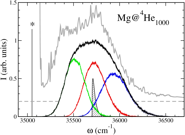
Figure 7: (Color online) Total absorption spectrum of one Mg atom attached to ⁴He₁₀₀₀ in the vicinity of the $3s3p$ ¹P${}_{1}\leftarrow 3s^{2}$ ¹S₀ transition. The line has been decomposed into its two $\Pi$ and one $\Sigma$ components, the former one is the higher frequency transition. The starred vertical line represents the gas-phase transition. The experimental curve, adapted for Ref. Reh00, , has been vertically offset for clarity. Also shown is the absorption spectrum obtained neglecting homogeneous broadening (hatched region)

Figure 7 shows the absorption spectrum of one Mg atom attached to ⁴He₁₀₀₀ in the vicinity of the $3s3p$ ¹P${}_{1}\leftarrow 3s^{2}$ ¹S₀ transition when homegeneous broadening is considered. We have decomposed the absorption line into its three components, the higher frequency component being the $\Sigma$ one. The starred vertical line represents the gas-phase transition, and the experimental curve, adapted from Ref. Reh00, , has been vertically offset for clarity. Also shown is the absorption spectrum obtained by neglecting homogeneous broadening (hatched region). This figure shows that the both the energy and width of the absorption peak that takes most of the experimental intensity are correctly described by our calculations.

V Two magnesium atoms attached to a ⁴He drop

The attachment of magnesium atoms in ⁴He droplets has been recently addressed using resonant two-photon-ionization.Prz07 In particular, the authors of Ref. Prz07, have obtained the absorption spectrum for drops doped with different, selected numbers of Mg atoms. From their measurements it appears that two main features contribute to the observed line shapes, one peaked at about 279 nm, and another at about 282 nm. This is in agreement with the results of Refs. Mor99, ; Reh00, (we recall that actually, the two peaks were not resolved by the authors of the bulk liquid experiment). The structure at 282 nm, however, only appears if the droplet contains more than one Mg atom. Thus the two-peak structure cannot be due to the splitting of the absorption line due to dynamical quadrupole deformations of the helium bubble around the impurity, as previously believed. We have indeed shown in the previous Section that this coupling only produces a broad peak, in good agreement with the results of Ref. Prz07, for helium drops containing just one Mg atom.

Another interesting observation reported in Ref. Prz07, is that their experimental results for multi-atom doped ⁴He droplets are not consistent with the formation of compact, metallic Mg clusters inside the ⁴He droplet. The magnesium atoms in the droplet appear instead to be relatively isolated from each other, showing only a weak interaction and leading to the 282 nm shift in the observation.

To confirm this scenario and find an explanation for the origin of the low energy component in the absorption peak, we have carried out DFT calculations to determine the structure of a two-magnesium doped ⁴He drop. Our goal is to verify whether the helium density oscillation around a magnesium atom may result in an energy barrier preventing the Mg atoms from merging into a Mg₂ dimer, as suggested by Przystawik et al.Prz07 To obtain the structure of two Mg atom in a ⁴He drop, we have minimized the energy of the system written as

$$E[\Psi,\Phi_{1},\Phi_{2}] = \frac{\hbar^{2}}{2\,m_{He}}\int\mathrm{d}^{3}\mathbf{r}\,|\nabla\Psi(\mathbf{r}\,)|^{2}+\int\mathrm{d}^{3}\mathbf{r}\,{\cal E}(\rho)$$ (27)

$$+ \frac{\hbar^{2}}{2\,m_{Mg}}\int\mathrm{d}^{3}\mathbf{r}\,\{|\nabla\Phi_{1}(\mathbf{r}\,)|^{2}+|\nabla\Phi_{2}(\mathbf{r}\,)|^{2}\}$$

$$+ \int\int\mathrm{d}^{3}\mathbf{r}\,\mathrm{d}^{3}\mathbf{r^{\prime}}\,\{|\Phi_{1}(\mathbf{r})|^{2}+|\Phi_{2}(\mathbf{r})|^{2}\}\,V_{Mg-He}(|\mathbf{r}-\mathbf{r^{\prime}}|)\,\rho(\mathbf{r^{\prime}})$$

$$+ \int\int\mathrm{d}^{3}\mathbf{r}\,\mathrm{d}^{3}\mathbf{r^{\prime}}\,|\Phi_{1}(\mathbf{r})|^{2}\,V_{Mg-Mg}(|\mathbf{r}-\mathbf{r^{\prime}}|)\,|\Phi_{2}(\mathbf{r^{\prime}})|^{2}\;,$$

where $V_{Mg-Mg}(|\mathbf{r}-\mathbf{r^{\prime}}|)$ is the Mg-Mg pair potential of Ref. Gue92, , and the other ingredients have the same meaning as in Eq. (1).

There are at least two additional effects which are not considered when modeling the Mg-Mg interaction via the pair-potential in vacuum, as implied in the above expression. The first is due to three-body (and higher) correlation effects involving the ⁴He atoms surrounding the Mg pair: these should exert an additional, albeit small, screening effect due to He polarization, which is expected to reduce the absolute value of the dispersion coefficients in the long-range part of the Mg-Mg interaction. The second is a possible reduction of the Mg atom polarizability due to the presence of the surrounding ⁴He cavity which, because of the repulsive character of the electron-He interaction, should make the electronic distribution of the impurity atom slightly “stiffer”, thus reducing further the values of the dispersion coefficients in the Mg-Mg pair interactions. Although in principle these effects might reduce the net interaction between a pair of Mg atoms embedded in liquid ⁴He, in practice in the present system they are indeed very small. The correction to the leading term of the long-range dispersion interaction, $-C_{6}/r^{6}$, due to three-body correlation effects can be written to first orderrenne as $-C_{6}(1-2\pi n\alpha/3)/r^{6}$, $\alpha$ being the static polarizability of the host fluid ($\alpha_{He}=1.39\,a_{0}^{3}$). Such correction is of the order of only 1% in our case. To estimate the change in the Mg atomic polarizability due to the surrounding He, we computed, using ab-initio pseudopotential calculations, the (static) polarizability of a Mg atom in the presence of an effective (mainly repulsive) potential acting on the Mg valence electrons due to the presence of the surrounding He. The effective interaction is derived from the equilibrium shape of the ⁴He bubble hosting the Mg atom, as predicted by our DFT calculations, and assuming a (local) electron-He density-dependent interaction which was proposed by Cole et al.Che94 We find a very small change in the static atomic polarizability $\alpha$ of Mg. Assuming that, roughly, $C_{6}\propto\alpha^{2}$ we find a reduction of the $C_{6}$ coefficient of about 1-2%.

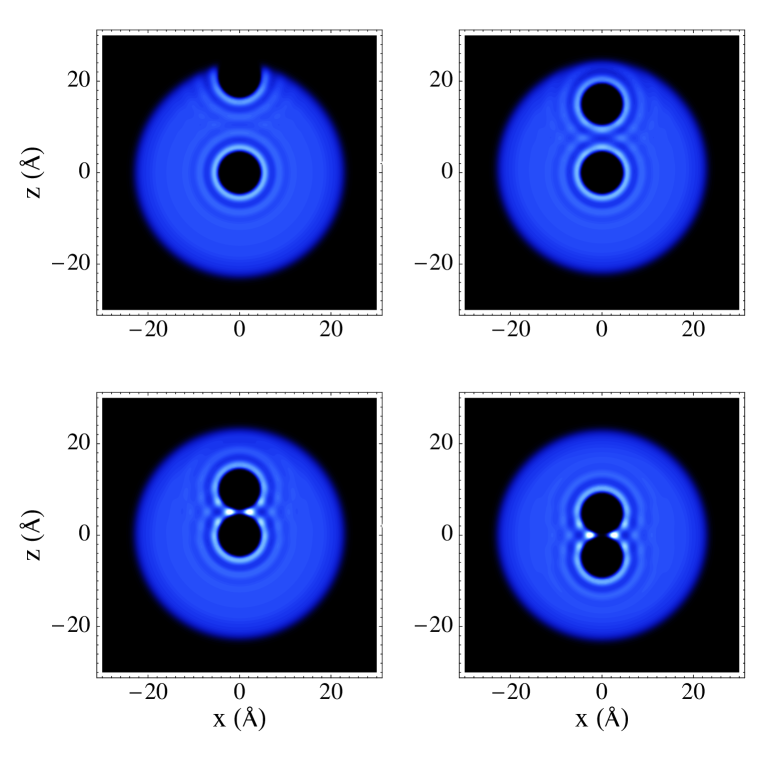
Figure 8: (Color online) From top to bottom and left to right, (Mg+Mg)@⁴He₁₀₀₀ metastable configurations for Mg-Mg interatomic distances $d=18.5$ Å, 12.9 Å, and 9.3 Å, and total energies -5567.8 K, -5573.9 K, and -5580.3 K, respectively. The bottom right panel shows the specularly symmetric configuration at $d=9.5$ Å with total energy $-5581.4$ K. The brigther regions are the higher density ones.

The minimisation of the total energy functional written above under the constraint of a given number of helium atoms and normalized Mg ground state wave functions should in principle yield the equilibrium configuration of the system. In practice, depending on the initial configuration, we have found several local minima, whose origin is again the “interference” of the He solvation shells around the Mg atoms. We have found three such metastable configurations for (Mg+Mg)@⁴He₁₀₀₀ if we start the minimization procedure with one Mg atom near the center of the droplet, and the other placed off center, at some distance from the first. They are displayed in Fig. 8. The energy difference between the innermost (Mg-Mg distance $d=9.3$ Å) and the outermost ($d=18.5$ Å) configurations is 12.5 K. The energy of the $d=9.3$ Å configuration is sensibly that of the configuration specularly symmetric about the $z=0$ plane (-5581.4 K) also shown in the figure. It is worth noticing that, since $R_{1/2}=22.2$ Å and the “radius” of Mg is $\sim 5$ Å, only the upper left corner configuration has the Mg impurity in a surface state.

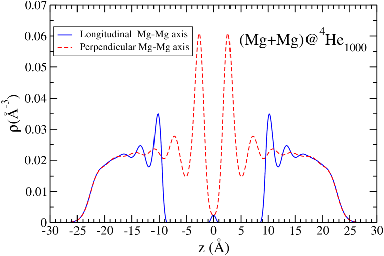
Figure 9: (Color online) Helium density profiles of the (Mg+Mg)@⁴He₁₀₀₀ symmetric configuration ($d=9.5$ Å) along the $z$-axis (solid line) and the $x$- or $y$-axis (dashed line).

Figure 9 shows two density profiles of the symmetric configuration obtained along the $z$-axis (solid line) and the $x$- or $y$-axis (dashed line). It shows a relatively high density helium ring around the two-bubble waist, clearly visible in Fig. 8, where the local density is almost three times the bulk liquid ⁴He density, and that prevents the collapse of the two-bubble configuration. The Mg wave functions are peaked at $\sim\pm 4.75$ Å, and very narrow. This justifies a posteriori the assumptions we have made to write the total energy of the system, Eq. (27).

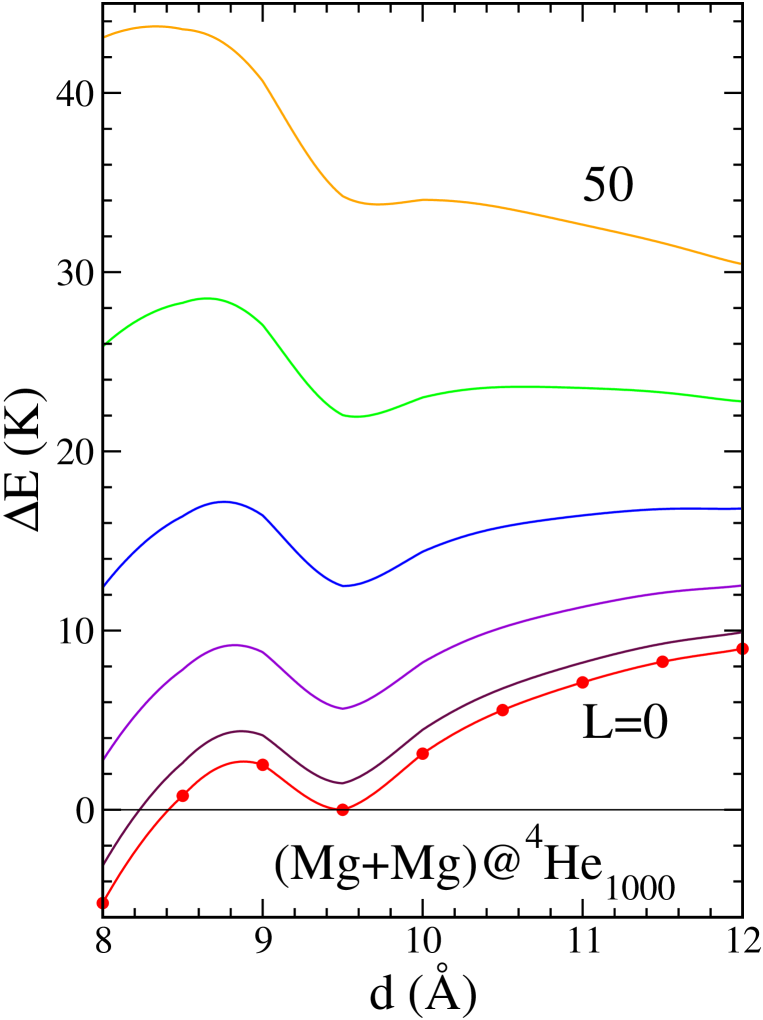
Figure 10: (Color online) Energy (K) of the Mg+Mg@⁴He₁₀₀₀ system as a function of the Mg-Mg distance (Å). The energies have been referred to that of the metastable equilibrium configuration (local minimum) at $L=0$. The lines have been obtained by a cubic spline of the actual calculations. From bottom to top, the curves correspond to $L=0$ to $50\hbar$ in $10\hbar$ steps.

Our results confirm the existence of the energy barrier suggested in Ref. Prz07, , that prevents the two Mg atoms from coming closer than some 9 Å, and thus hindering, at least temporarily, the formation of the Mg₂ dimer. This barrier is shown in Fig. 10 as a function of the Mg-Mg distance $d$, which is kept fixed in a constrained energy minimization. Note that the energy of the Mg+Mg system increases as $d$ does because the two Mg atoms in a drop form a state more bound than that of a pure drop with the impurities well apart.

Since the height of the barrier is larger than the experimental temperatures, $T\sim 0.4\,K$, two solvated Mg atoms will not easily merge into a dimer, but rather form of a metastable weakly bound state. Based on these finding, we suggest that several Mg atoms solvated inside ⁴He drops might form a sparse, weakly-bound “foam”-like aggregate rather than coalesce into a more tightly bound metallic cluster. Partial coagulation of impurities was already invoked by Toennies and coworkers to explain their experimental findings for the successive capture of foreing atoms and molecules in helium clustersLew95 (see also Ref. Gor04, for the case of bulk liquid helium). Very recently, a kind of “quantum gel” has been predicted to be formed in ⁴He drops doped with neon atoms.Elo08 Although some degree of mutual isolation between foreign atoms is expected in the case of strongly attractive impurities (like those studied in the two cases mentioned above), where they are kept apart by the presence a solid ⁴He layer coating the impurity,Gor04 our calculations show that this effect is possible even for relatively weakly attractive impurities like Mg, where such solid-like ⁴He layer is absent.

One may estimate the mean life of the metastable state as

$$\tau=2\pi\sqrt{\frac{\mu^{*}_{Mg}}{U^{\prime\prime}(d_{eq})}}\,\exp{[\Delta U/(k_{B}T)]}\;,$$ (28)

where $\mu^{*}_{Mg}=M^{*}_{Mg}/2\sim 20$ a.u. is the hydrodynamic reduced mass of the Mg+Mg system and $\Delta U$ is the barrier height. From Fig. 10 we have that $U^{\prime\prime}(d_{eq})\sim 40$ K Å^-2. This yields a mean life of a few nanoseconds, which is about five to six orders of magnitude smaller than the time needed for its experimental detection.Prz07 ; Notabarrier The mean life becomes increasingly large as the relative angular momentum $L$ deposited into the two Mg system increases. Writing

$$\Delta E=\Delta E(L=0)+\frac{\hbar^{2}}{2\mu^{*}_{Mg}}\frac{L(L+1)}{d^{2}}\;,$$ (29)

one obtains the $L-$dependent energy barriers displayed in Fig. 10. For $L=30$ we have $\tau\sim 0.6$ $\mu$s, and for $L=40$, $\tau\sim 0.1$ milliseconds. Thus, there is an angular momentum window that may yield mean lifes compatible with the experimental findings. Increasing $L$ much further would produce too a distant Mg+Mg system which would correspond to a two independent Mg impurities in a drop.

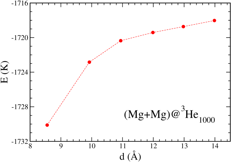
Figure 11: (Color online) Energy (K) of the Mg+Mg@³He₁₀₀₀ system as a function of the Mg-Mg distance (Å). The line has been drawn to guide the eye.

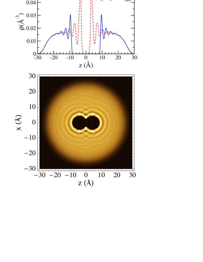
Figure 12: (Color online) Top panel: helium density profiles of the (Mg+Mg)@³He₁₀₀₀ complex at $d=8.6$ Å along the $z$-axis (solid line) and the $x$- or $y$-axis (dashed line). Bottom panel: equidensity lines corresponding to the same configuration. The brigther regions are the higher density ones.

To check whether this foam-like structure of the Mg aggregate also appears in ³He drops, we have carried out calculations for (Mg+Mg)@³He₁₀₀₀ using the same density functional as in Ref. Sti04, , and the method presented in this Section. Figure 11 shows the energy of the (Mg+Mg)@³He₁₀₀₀ complex as a function of $d$. For distances smaller than some 8.6 Å we have found that the system has a tendency to collapse into a dimer -physically unreachable from our starting point, Eq. (27). We are led to conclude that there is no barrier in the case of liquid ³He. The configuration corresponding to the closest $d$ we have calculated is shown in Fig. 12.

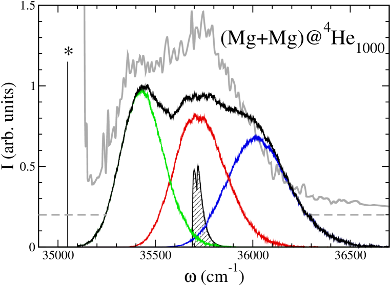
Figure 13: (Color online) Total absorption spectrum of one Mg atom attached to ⁴He₁₀₀₀ in the vicinity of the $3s3p$ ¹P${}_{1}\leftarrow 3s^{2}$ ¹S₀ transition in the distorted environment created by the presence of another Mg atom. The line has been decomposed into its two $\Pi$ and one $\Sigma$ components, the former one is the higher frequency transition. The starred vertical line represents the gas-phase transition. The experimental curve, adapted for Ref. Reh00, , has been vertically offset for clarity. Also shown is the absorption spectrum obtained neglecting homogeneous broadening (hatched region)

We are now in the position to determine the effect of these weakly-bound systems on the LIF and R2PI experiments on ⁴He droplets containing more than one Mg atom. Notice that the bottom right panel of Fig. 8 shows that the helium bubbles have a non-zero static quadrupole moment, whereas they are spherically symmetric for one single Mg atom in the drop. It is precisely the existence of this static quadrupole moment that causes an additional separation between the $\Sigma$ and $\Pi$ spectral components in the absorption spectra, which results, as a consequence of the broadening of each line, in an double-peak structure of the computed spectra, in semi-quantitative agreement with the experimental data. Details of our calculation are given in Appendix C, see Eq. (82). Figure 13 shows such two-peak structure corresponding to the specularly symmetric configuration displayed in Fig. 8, and indicates that the 282 nm structure observed in the experiments may be attributed to the distortion produced by neighbour Mg bubbles; these bubbles contribute incoherently to the absorption spectrum, and the relative intensity of the 282 and 279 nm peaks might reflect the different population of drops doped with one and two Mg atoms, since those hosting a compact cluster (dimer, trimer, etc), would not yield an absorption signal in the neighborhood of the monomer $3s3p$ ¹P${}_{1}\leftarrow 3s^{2}$ ¹S₀ transition. Notice that a large static distortion of the helium bubble could also arise if the Mg atom were in a shallow dimple at the drop surface, but Fig. 6 discards this possibility.

We finally note that we have not considered in our work another source for an additional splitting of the spectral lines of a Mg atom in the field produced by a neighboring one, i.e. the resonant dipole-dipole interaction occurring during the electronic excitation. This effect could in principle lead to an additional (but probably small, compared with the effect discussed here) splitting of the calculated lines. An accurate determination of the dipole moment is required for a proper inclusion of this effect, which is beyond the scope of the present paper.

VI Summary

We have obtained, within DFT, the structure of ⁴He droplets doped with Mg atoms and have discussed in detail the magnesium solvation properties. In agreement with previous DMC calculations,Mel05 ; Elh08 we have found that Mg is not fully solvated in small ⁴He drops, whereas it becomes fully solvated in large droplet.

As a consequence of its interaction with the helium environment, it turns out that magnesium is radially quite delocalized inside the droplets. This large delocalization provides a way to reconcile two contradictory results on the solution of one Mg atom in a ⁴He drop, namely center localization (LIF and R2PI experimentsReh00 ; Prz07 ), and surface localization (electron-impact ionization experimentsRen07 ).

We have calculated the absorption spectrum of magnesium in the vicinity of the $3s3p$ ¹P${}_{1}\leftarrow 3s^{2}$ ¹S₀ transition. For the large Mg@⁴He₁₀₀₀ droplet, where Mg is fully solvated, we reproduce the more intense component of the absorption line found by LIF and R2PI experiments in large drops and in liquid helium. This agreement is only achieved when homegeneous broadening due to the coupling of the dipole excitation with the quadrupole deformations of the helium bubble are fully taken into account. This coupling is naturally included in Quantum Monte Carlo simulations of the absorption spectrum,Oga99 ; Mel02 whereby one takes advantage of the inherent fluctuations present in these simulations. These fluctuations are the full quantal equivalent of the dynamical distortions of the helium bubble we have introduced for the description of homogeneous broadening. An alternative method to include shape fluctuations within DFT has been proposed and applied to the case of Cs in bulk liquid helium.Nak02 It would be interesting to adapt this method to the drop geometry, since it is not simple to handle dynamical bubble distortions in a non-spherical environment, or in ³He drops.

To explain the origin of the low energy peak in the absorption line and confirm the likely existence of soft, “foam”-like structure of Mg aggregates in ⁴He drops as proposed by Przystawik et al,Prz07 we have addressed the properties of two Mg atoms in ⁴He₁₀₀₀ and have found that indeed, Mg atoms are kept apart by the presence of helium atoms that prevent the formation of a compact Mg cluster. We have estimated that the height of the energy barrier for the formation of the Mg dimer in ⁴He drops is $\sim 2-3$ K, which should be enough, at the droplet experimental temperature of $0.4$ K, to guarantee a relatively long lifetime to these weakly-bound Mg aggregates. We predict that, contrarily, Mg atoms adsorbed in ³He droplets do not form such metastable states.

The presence of neighboring Mg atoms in these structures induces a static quadrupole deformation in the helium bubble accomodating a Mg atom. As a consequence, the dipole absorption line around the $3s3p$ ¹P${}_{1}\leftarrow 3s^{2}$ ¹S₀ transition splits. We attribute to this static quadrupole moment the origin of the low energy peak in the absorption line, and confirm the suggestion made by the Rostock group Prz07 that the splitting of the absorption line, rather than being due to a dynamical (Jahn-Teller) deformation of the helium bubble, is due to the presence of more than one magnesium atom in the same droplet.

Our previous study on Ca doped helium dropsHer08 and the present work show that DFT is able to quantitatively address the dipole absorption of dopants in ⁴He drops within the diatomics-in-molecules approach, provided the impurity-helium pair potentials are accurately determined. However, we want to point out that, while we have a consistent scenario that explains the results of LIF and R2PI experiments, the understanding of the electron-impact ionization experiment reported in Ref. Ren07, still requires further analysis. Indeed, since Mg atoms may be in the bulk of the drop or just beneath the drop surface, the experimental ion yield curve should reflect both possibilities, whereas apparently it does not (see Fig. 2 of Ref. Ren07, ). One possible explanation may be that for electron-impact experiments, a $N=10\,000$ drop is still small, so that the impurity is always close enough to the drop surface to make the Penning ionization process to prevail on the direct formation of a He⁺ ion.

Appendix A

In this Appendix we obtain the energy of the doped drop up to second order in the deformation parameters and the hydrodynamic mass of the helium bubble. To this end, the helium order parameter and Mg wave function are expressed as $\Psi(\mathbf{r},t)=\sqrt{\rho(\mathbf{r},t)}\exp[i\frac{m_{He}}{\hbar}S(\mathbf{r},t)]$ and $\Phi(\mathbf{r},t)=|\Phi(\mathbf{r},t)|\exp[i\frac{m_{Mg}}{\hbar}\varphi(\mathbf{r},t)]$, respectively. Neglecting the velocity-dependent terms of the Orsay-Trento functional that mimic backflow effects,Dal95 the total energy of the system is written as

$$E =\frac{1}{2}m_{He}\int\mathrm{d}^{3}\mathbf{r}\,\rho(\mathbf{r},t)|\nabla S(\mathbf{r},t)|^{2}+\frac{1}{2}m_{Mg}\int\mathrm{d}^{3}\mathbf{r}\,|\Phi(\mathbf{r},t)|^{2}|\nabla\varphi(\mathbf{r},t)|^{2}$$ (30)

$$+ \frac{\hbar^{2}}{2\,m_{He}}\int\mathrm{d}^{3}\mathbf{r}\,|\nabla\sqrt{\rho(\mathbf{r},t)}|^{2}+\frac{\hbar^{2}}{2\,m_{Mg}}\int\mathrm{d}^{3}\mathbf{r}\,\left|\nabla|\Phi(\mathbf{r},t)|\right|^{2}+\int\mathrm{d}^{3}\mathbf{r}\,{\cal E}(\rho)$$

$$+ \int\int\mathrm{d}^{3}\mathbf{r}\,\mathrm{d}^{3}\mathbf{r^{\prime}}\,|\Phi(\mathbf{r},t)|^{2}\,V_{Mg-He}(|\mathbf{r}-\mathbf{r^{\prime}}|)\,\rho(\mathbf{r^{\prime}},t)\;,$$

where the functions $\rho$($|\Phi|$) and $S$($\varphi$) fulfill the continuity equations

$$-\frac{\partial}{\partial t}\rho(\mathbf{r},t) = \nabla\left[\rho(\mathbf{r},t)\nabla S(\mathbf{r},t)\right]$$ (31)

$$-\frac{\partial}{\partial t}|\Phi(\mathbf{r},t)|^{2} = \nabla\left[|\Phi(\mathbf{r},t)|^{2}\nabla\varphi(\mathbf{r},t)\right]$$ (32)

that allow to identify $S(\mathbf{r},t)$ and $\varphi(\mathbf{r},t)$ as velocity field potentials, and the first two terms in Eq. (30) as a collective kinetic energy, whose density we denote as $t[\rho,S,|\Phi|,\varphi]$. Thus,

$$E=T+V=\int\mathrm{d}^{3}\mathbf{r}\left\{t[\rho,S,|\Phi|,\varphi]+v[\rho,|\Phi|]\right\}\;.$$ (33)

In the adiabatic approximation, the dynamics of the system requires the following steps: i) introduce a set of collective variables (or deformation parameters) $[\alpha(t)])$ that define the helium density, $\rho(\mathbf{r},t)=\rho(\mathbf{r},[\alpha(t)])$; ii) for each helium configuration defined by $[\alpha]$, solve the time-independent Schrödinger equation obeyed by $|\Phi(\mathbf{r},[\alpha])|$; iii) obtain the potential surface $V[\rho,|\Phi|]$ by computing the static energy for each configuration; iv) determine the velocity field potentials $S(\mathbf{r},[\alpha(t)])$ and $\varphi(\mathbf{r},[\alpha(t)])$ by solving the continuity equations; v) compute the collective kinetic energy to obtain the hydrodynamic mass, and vi) solve the equation of motion associated with the effective Hamiltonian written as a function the deformation parameters.

We aim to describe harmonic deformations of a spherical helium bubble created by an impurity in the ground state, and have to determine the helium density $\rho(\mathbf{r},[\alpha(t)])$ resulting from a change in the radial distance to the center of the spherical bubble induced by the $[\alpha(t)]$ parameters:

$$r\longrightarrow r+\sum_{\lambda=0}^{\infty}\sum_{\mu=-\lambda}^{\lambda}\alpha_{\lambda\mu}(t)Z_{\lambda\mu}(\widehat{r})\;,$$ (34)

where the $\lambda=1$ deformation is now introduced to allow for displacements of the bubble. We recall that the real spherical harmonics have been normalized as $\langle Z_{\lambda\mu}|Z_{\lambda^{\prime}\mu^{\prime}}\rangle=\frac{4\pi}{2\lambda+1}\delta_{\lambda\lambda^{\prime}}\delta_{\mu\mu^{\prime}}$, with $Z_{00}(\widehat{r})=1$, $Z_{10}(\widehat{r})=\cos\theta$, etc. The breathing mode corresponds to $\lambda=0$, an infinitesimal translation to $\lambda=1$ (provided the fluid is incompressible), and a quadrupolar deformation to $\lambda=2$. To first order, the density can be written as

$$\rho(\mathbf{r},t)\simeq\rho_{0}(r)+\rho_{0}^{\prime}(r)\sum_{\lambda=0}^{\infty}\sum_{\mu=-\lambda}^{\lambda}\alpha_{\lambda\mu}(t)Z_{\lambda\mu}(\widehat{r})\;,$$ (35)

where from now on, the prime will denote the derivative of the function with respect to its argument.

A.1 Impurity wave function

To first order, the wave function $|\Phi(\mathbf{r},[\alpha])|$ is written as

$$|\Phi(\mathbf{r},t)|\simeq\Phi_{0}(r)+\sum_{\lambda=0}^{\infty}\sum_{\mu=-\lambda}^{\lambda}\alpha_{\lambda\mu}(t)\Phi^{(1)}_{\lambda\mu}(\mathbf{r})\;.$$ (36)

The amplitudes $\Phi^{(1)}_{\lambda\mu}(\mathbf{r})$ are determined in first order perturbation theory from the multipole expansion of the impurity-helium pair potential

$$U^{(1)}_{\lambda\mu}(\mathbf{r}) = \int\mathrm{d}^{3}\mathbf{r}^{\prime}\rho_{0}^{\prime}(r^{\prime})Z_{\lambda\mu}(\widehat{r}^{\prime})V_{X-He}(|\mathbf{r}-\mathbf{r^{\prime}}|)$$ (37)

$$= \int\mathrm{d}^{3}\mathbf{r}^{\prime}\rho_{0}^{\prime}(r^{\prime})Z_{\lambda\mu}(\widehat{r}^{\prime})\sum_{\lambda\mu}V_{X-He}^{\lambda}(r,r^{\prime})Z_{\lambda\mu}(\widehat{r})Z_{\lambda\mu}(\widehat{r}^{\prime})$$

$$\equiv U^{(1)}_{\lambda}(r)Z_{\lambda\mu}(\widehat{r})\;,$$

which defines $U^{(1)}_{\lambda}(r)$. We obtain

$$\Phi^{(1)}_{\lambda\mu}(\mathbf{r}) = \sum_{n\ell m}\frac{\langle\Phi_{0}|U^{(1)}_{\lambda}Z_{\lambda\mu}|\Phi_{n\ell}Z_{\ell m}\rangle}{\varepsilon_{0}-\varepsilon_{n\ell m}}\Phi_{n\ell}(r)Z_{\ell m}(\widehat{r})$$ (38)

$$= \left[\sum_{n}\frac{4\pi}{2\lambda+1}\frac{\langle\Phi_{0}|U^{(1)}_{\lambda}|\Phi_{n\lambda}\rangle}{\varepsilon_{0}-\varepsilon_{n\lambda\mu}}\Phi_{n\lambda}(r)\right]Z_{\lambda\mu}(\widehat{r})$$

$$\equiv \Phi^{(1)}_{\lambda}(r)Z_{\lambda\mu}(\widehat{r})$$

that shows that actually, $\Phi^{(1)}_{\lambda\mu}$ is $\mu$ independent.

Once we have obtained the wave function, we can compute the energy surface $V[\rho,|\Phi|]$. Since we describe deformations around a spherically symmetric ground state, the first order term vanishes, and the derivative $g_{\lambda}\equiv\partial^{2}v/\partial\alpha_{\lambda\mu}\partial\alpha_{\lambda^{\prime}\mu^{\prime}}$ is also spherically symmetric. We can evaluate the second order contribution to the collective potential energy as

$$V^{(2)} = \sum_{\lambda\mu}\sum_{\lambda^{\prime}\mu^{\prime}}\frac{1}{2}\int\mathrm{d}^{3}\mathbf{r}\left.\frac{\partial^{2}v}{\partial\alpha_{\lambda\mu}\partial\alpha_{\lambda^{\prime}\mu^{\prime}}}\right|_{\rho_{0},\varphi_{0}}\alpha_{\lambda\mu}Z_{\lambda\mu}(\widehat{r})\alpha_{\lambda^{\prime}\mu^{\prime}}Z_{\lambda^{\prime}\mu^{\prime}}(\widehat{r})$$ (39)

$$= \sum_{\lambda\mu}\frac{2\pi}{2\lambda+1}\int_{0}^{\infty}\mathrm{d}r\,r^{2}g_{\lambda}(r)\alpha_{\lambda\mu}^{2}$$

$$\equiv \sum_{\lambda=0}^{\infty}\frac{2\pi}{2\lambda+1}E^{(2)}_{\lambda}\sum_{\mu=-\lambda}^{\lambda}\alpha_{\lambda\mu}^{2}\;,$$

which defines $E^{(2)}_{\lambda}$. The parameters $[\alpha]$ are the dynamical variables that describe the evolution of the system.

A.2 Velocity field potentials

Introducing the expansion $S(\mathbf{r},t)\equiv\sum_{\lambda\mu}\dot{\alpha}_{\lambda\mu}(t)\tilde{S}_{\lambda}(r)Z_{\lambda\mu}(\widehat{r})$, where the dot denotes the time-derivative, the continuity equation for the liquid helium is, to first order,

$$-\sum_{\lambda\mu}\dot{\alpha}_{\lambda\mu}~{}Z_{\lambda\mu}~{}\frac{\mathrm{d}\rho_{0}}{\mathrm{d}r}=\sum_{\lambda\mu}\dot{\alpha}_{\lambda\mu}~{}Z_{\lambda\mu}\left\{\frac{\mathrm{d}\rho_{0}}{\mathrm{d}r}\frac{\mathrm{d}\tilde{S}_{\lambda}}{\mathrm{d}r}+\rho_{0}\left[\frac{\mathrm{d}^{2}\tilde{S}_{\lambda}}{\mathrm{d}r^{2}}+\frac{2}{r}\frac{\mathrm{d}\tilde{S}_{\lambda}}{\mathrm{d}r}-\frac{\lambda(\lambda+1)}{r^{2}}\tilde{S}_{\lambda}\right]\right\}\;.$$ (40)

Hence,

$$-\frac{\mathrm{d}\rho_{0}}{\mathrm{d}r}=\frac{\mathrm{d}\rho_{0}}{\mathrm{d}r}\frac{\mathrm{d}\tilde{S}_{\lambda}}{\mathrm{d}r}+\rho_{0}\left[\frac{\mathrm{d}^{2}\tilde{S}_{\lambda}}{\mathrm{d}r^{2}}+\frac{2}{r}\frac{\mathrm{d}\tilde{S}_{\lambda}}{\mathrm{d}r}-\frac{\lambda(\lambda+1)}{r^{2}}\tilde{S}_{\lambda}\right].$$ (41)

When $r\rightarrow\infty$, the density vanishes for a drop, and approaches $\rho_{b}$ for the liquid. In the later case, Eq. (41) reduces to the radial part of the Laplace equation

$$0=\frac{\mathrm{d}^{2}\tilde{S}_{\lambda}}{\mathrm{d}r^{2}}+\frac{2}{r}\frac{\mathrm{d}\tilde{S}_{\lambda}}{\mathrm{d}r}-\frac{\lambda(\lambda+1)}{r^{2}}\tilde{S}_{\lambda}$$ (42)

whose general solution is

$$\tilde{S}_{\lambda}(r)=A_{\lambda}~{}r^{\lambda}+\frac{B_{\lambda}}{r^{\lambda+1}}\;.$$ (43)

We have solved Eq. (41) adapting the method proposed in Ref. Leh02, . Let $r_{i}$ be the first point where $\rho_{0}(r)$ is significantly different from zero $[\rho_{0}(r)=0\,\,{\rm for}\,\,r\leq r_{i}]$. At this point, Eq. (41) implies that

$$\left.-\frac{\mathrm{d}\rho_{0}}{\mathrm{d}r}\right|_{r_{i}}=\left.\frac{\mathrm{d}\rho_{0}}{\mathrm{d}r}\frac{\mathrm{d}\tilde{S}_{\lambda}}{\mathrm{d}r}\right|_{r_{i}},$$ (44)

which determines the boundary condition at $r_{i}$:

$$\left.\frac{\mathrm{d}\tilde{S}_{\lambda}}{\mathrm{d}r}\right|_{r_{i}}=-1\;.$$ (45)

For the liquid, the other boundary condition is that when $r\rightarrow\infty$, the solution behaves as in Eq. (43) with $A_{\lambda}=0$ to have a physically acceptable solution. If the bubble has a sharp surface of radius $r_{i}$ and the liquid is uniform, $\tilde{S}_{\lambda}(r)$ is completely determined by Eq. (43) and the velocity field potential that fulfills Eq. (45) corresponds to the coefficients

$$A_{\lambda} = 0$$

$$B_{\lambda} = \frac{r_{i}^{\lambda+2}}{\lambda+1}\;.$$ (46)

To find the velocity field potential in a large drop, we have defined a radial distance $r_{b}$, far from the bubble and from the drop surface at $R_{1/2}$, around which on one may consider that the density is that of the liquid. Starting from $r=r_{b}$ with the liquid solution fixed by the coefficients given in Eq. (46), we have integrated inwards Eq. (41), finding the solutions $\tilde{S}_{\lambda}^{\mathrm{inh}}(r)$ and $\tilde{S}_{\lambda}^{\mathrm{h}}(r)$ that correspond, respectively, to the non-homegeneous and to the homegeneous differential equation that results by setting to zero the left hand side of Eq. (41). The general solution that satisfy the boundary condition Eq. (45) is obtained as

$$\tilde{S}_{\ell}(r)=\tilde{S}_{\lambda}^{\mathrm{inh}}(r)+C\tilde{S}_{\lambda}^{\mathrm{h}}(r)$$ (47)

with

$$C=-\frac{1+\left.\frac{\mathrm{d}\tilde{S}_{\lambda}^{\mathrm{inh}}}{\mathrm{d}r}\right|_{r_{i}}}{\left.\frac{\mathrm{d}\tilde{S}_{\lambda}^{\mathrm{h}}}{\mathrm{d}r}\right|_{r_{i}}}\;.$$ (48)

The field $\varphi$ is analogously obtained after introducing the expansion $\varphi(\mathbf{r},t)=\sum_{\lambda\mu}\dot{\alpha}_{\lambda\mu}(t)\tilde{\varphi}_{\lambda}(r)\mathcal{Z}_{\lambda\mu}(\widehat{r})$. We have assumed that the wave function of the impurity in the ground state is a Gaussian $\Phi_{0}(r)=A\exp\left(-\beta r^{2}\right)$ whose shape has been determined by fitting it to the actual wave function, and have introduce a cutoff distance $r_{g}$ such that safely $\Phi_{0}(r)=0$ if $r\geq r_{g}$. We then obtain the following differential equation to determine $\tilde{\varphi}_{\lambda}$:

$$4\beta r=-4\beta r\frac{\mathrm{d}\tilde{\varphi}_{\lambda}}{\mathrm{d}r}+\frac{\mathrm{d}^{2}\tilde{\varphi}_{\lambda}}{\mathrm{d}r^{2}}+\frac{2}{r}\frac{\mathrm{d}\tilde{\varphi}_{\lambda}}{\mathrm{d}r}-\frac{\lambda(\lambda+1)}{r^{2}}\tilde{\varphi}_{\lambda}\;.$$ (49)

The appropriate boundary conditions are

$$\left.\frac{\mathrm{d}\tilde{\varphi}_{\lambda}}{\mathrm{d}r}\right|_{r_{0}} = -1$$

$$\tilde{\varphi}_{\lambda}(0) = 0\;,$$ (50)

and the solution is analytical but very involved (we have found it by using the Mathematica packpage). The dipole mode is the only exception; if $\lambda=1$ we have $\tilde{\varphi}_{1}=-r$.

A.3 Kinetic energy

Once the velocity fields $S(\mathbf{r},t)$ and $\varphi(\mathbf{r},t)$ have been determined, the collective kinetic energy can be easily calculated to second order in the collective parameters:

$$T = \int\mathrm{d}^{3}\mathbf{r}~{}t[\rho,S,|\Phi|,\varphi]$$ (51)

$$= \frac{1}{2}m_{He}\int\mathrm{d}^{3}\mathbf{r}\,\rho(\mathbf{r},t)|\nabla S(\mathbf{r},t)|^{2}+\frac{1}{2}m_{Mg}\int\mathrm{d}^{3}\mathbf{r}\,|\Phi(\mathbf{r},t)|^{2}|\nabla\varphi(\mathbf{r},t)|^{2}$$

$$\simeq \sum_{\lambda=0}^{\infty}\frac{4\pi}{2\lambda+1}\left\{\frac{1}{2}m_{He}\int\mathrm{d}r~{}r^{2}~{}\rho_{0}(r)~{}\left[\left(\frac{\mathrm{d}\tilde{S}_{\lambda}}{\mathrm{d}r}\right)^{2}+\frac{\lambda(\lambda+1)}{r^{2}}\tilde{S}_{\lambda}^{2}\right]\right.$$

$$\left.+\frac{1}{2}m_{Mg}\int\mathrm{d}r~{}r^{2}~{}|\Phi_{0}(r)|^{2}~{}\left[\left(\frac{\mathrm{d}\tilde{\varphi}_{\lambda}}{\mathrm{d}r}\right)^{2}+\frac{\lambda(\lambda+1)}{r^{2}}\tilde{\varphi}_{\lambda}^{2}\right]\right\}\sum_{\mu=-\lambda}^{\lambda}\dot{\alpha}_{\lambda\mu}^{2}$$

$$\equiv \frac{1}{2}\sum_{\lambda=0}^{\infty}M_{\lambda}^{*}\sum_{\mu=-\lambda}^{\lambda}\dot{\alpha}_{\lambda\mu}^{2}$$

which defines the hydrodynamic mass $M_{\lambda}^{*}$ for each $\lambda$ mode.

Using the continuity equations and the Gauss theorem, one can find an alternative expression for $M_{\lambda}^{*}$

$$M_{\lambda}^{*}=\frac{4\pi}{2\lambda+1}\left\{m_{He}\int\mathrm{d}r~{}r^{2}~{}\rho^{\prime}_{0}(r)~{}\tilde{S}_{\lambda}(r)+m_{Mg}\int\mathrm{d}r~{}r^{2}~{}2\Phi_{0}(r)\Phi^{\prime}_{0}(r)\tilde{\varphi}_{\lambda}(r)\right\}\;.$$ (52)

We have checked that both expressions yield the same values for $M_{\lambda}^{*}$, which constitutes a test on the numerical accuracy of the method. It is easy to see from Eq. (51) that in bulk liquid helium, the $\lambda=1$ hydrodynamic mass coincides with that given in Ref. Leh02, . Using that $\tilde{\varphi}_{1}=-r$, it is also easy to check from the above expressions that the impurity contribution to the $\lambda=1$ hydrodynamic mass is just the bare mass of the Mg atom.

The sum of Eqs. (39) and (51) represents the Hamiltonian of a set of uncoupled harmonic oscillators whose frequency only depends on $\lambda$.

Appendix B

In this Appendix we work out in detail the expressions we have used to describe the homogeneous broadening of the absorption line. We consider a spherical ground state defined by a helium density $\rho_{0}(r)$ and impurity wave function $\Phi_{0}(r)$, both modified by the action of the breathing mode defined in Eq. (21), namely $\rho(r,\alpha_{0})=\rho_{0}(r+\alpha_{0})\,{\cal K}^{-1}$, and $\Phi(r,\alpha_{0})$. The computation of the spectra for a given $\alpha_{0}$ can be carried out starting from Eq. (11)

$$I(\omega,\alpha_{0})=4\pi\sum_{i}\int\mathrm{d}r~{}|r~{}\Phi(r,\alpha_{0})|^{2}\delta[\omega+\omega(\alpha_{0})-V^{\mathrm{ex}}_{i}(r,\alpha_{0})/\hbar]\;,$$ (53)

where $\hbar\omega(\alpha)=\varepsilon(\alpha_{0})$ is the impurity eigenenergy and $V^{\mathrm{ex}}_{i}(r,\alpha_{0})$ are the PES defined by Eq. (13), where $[\alpha]$ reduces to $\alpha_{0}$. Notice that $\alpha_{0}$ is not introduced perturbatively; it is unnecessary since this mode does not break the spherical symmetry. Next, we perturbatively introduce the modes with $\lambda\geq 2$ to first order; Eq. (53) becomes

$$I(\omega,[\alpha]) \simeq I(\omega,\alpha_{0})$$ (54)

$$+\sum_{i}\sum_{\lambda=2}^{\infty}\sum_{\mu=-\lambda}^{\lambda}\left\{\int\mathrm{d}\mathbf{r}~{}\Phi(r,\alpha_{0})\Phi^{(1)}_{\lambda}(r,\alpha_{0})Z_{\lambda\mu}(\hat{r})\delta[\omega+\omega(\alpha_{0})-V^{\mathrm{ex}}_{i}(r,\alpha_{0})/\hbar]\right.$$

$$\left.-4\pi\int\mathrm{d}r~{}|r~{}\Phi(r,\alpha_{0})|^{2}\delta^{\prime}[\omega+\omega(\alpha_{0})-V^{\mathrm{ex}}_{i}(r,\alpha_{0})/\hbar]\frac{1}{\hbar}\epsilon_{\lambda\mu}^{i}(r)\right\}\alpha_{\lambda\mu}\;,$$

where $\epsilon_{\lambda\mu}^{i}(r)=\left.\partial V^{\mathrm{ex}}_{i}(r)/\partial\alpha_{\lambda\mu}\right|_{[\alpha]_{\lambda\geq 2}=0}$. The first integral is zero due to the orthogonality of the spherical harmonics. To evalue the second integral, we expand $\epsilon_{\lambda\mu}^{i}(r)$ as a power series of $r$. Taken into account that the PES have a stationary point at $r=0$ due to the spherical geometry –the first order term is zero– we can safely stop the expansion at the zeroth order term, since the wave function $\Phi(r,\alpha_{0})$ is very narrow

$$I(\omega,[\alpha])\simeq I(\omega,\alpha_{0})$$

$$-4\pi\sum_{i}\sum_{\lambda=2}^{\infty}\sum_{\mu=-\lambda}^{\lambda}\int\mathrm{d}r~{}|r~{}\Phi(r,\alpha_{0})|^{2}\delta^{\prime}[\omega-\omega(\alpha_{0})-V^{\mathrm{ex}}_{i}(r,\alpha_{0})/\hbar]\left(\frac{1}{\hbar}\epsilon_{\lambda\mu}^{i}(0)\alpha_{\lambda\mu}\right)\;.$$ (55)

This equation may be interpreted as the expansion to first order of a shift in $\omega$, so it can be written as

$$I(\omega,[\alpha]) \simeq 4\pi\sum_{i}\int\mathrm{d}r~{}|r~{}\Phi(r,\alpha_{0})|^{2}\delta\left[\omega+\omega(\alpha_{0})-\frac{1}{\hbar}\left(V^{\mathrm{ex}}_{i}(r,\alpha_{0})+\sum_{\lambda=2}^{\infty}\sum_{\mu=-\lambda}^{\lambda}\epsilon_{\lambda\mu}^{i}(0)\alpha_{\lambda\mu}\right)\right]$$ (56)

$$= \sum_{i}I\left[\omega+\sum_{\lambda=2}^{\infty}\sum_{\mu=-\lambda}^{\lambda}\epsilon_{\lambda\mu}^{i}(0)\alpha_{\lambda\mu}/\hbar,\alpha_{0}\right]\;.$$

Thus the eigenvalues $\epsilon_{\lambda\mu}^{i}(0)$ are related to the diagonalization of the expansion of $U_{ij}(\mathbf{r},[\alpha])$ defined in Eq. (12). Writing this matrix equation as a function of the real spherical harmonics

$$U(\mathbf{r},[\alpha])=\int\mathrm{d}^{3}\mathbf{r^{\prime}}\rho(\mathbf{r^{\prime}}+\mathbf{r},[\alpha])\left\{\frac{1}{3}[V_{\Sigma}(r^{\prime})+2V_{\Pi}(r^{\prime})]Z_{00}(\hat{r})\left(\begin{array}[]{ccc}1&0&0\\ 0&1&0\\ 0&0&1\end{array}\right)\right.$$ (60)

$$\left.+\frac{1}{\sqrt{3}}[V_{\Sigma}(r^{\prime})-V_{\Pi}(r^{\prime})]\left(\begin{array}[]{ccc}-\frac{1}{\sqrt{3}}Z_{20}(\hat{r})+Z_{22}(\hat{r})&Z_{2-2}(\hat{r})&Z_{21}(\hat{r})\\ Z_{2-2}(\hat{r})&-\frac{1}{\sqrt{3}}Z_{20}(\hat{r})-Z_{22}(\hat{r})&Z_{2-1}(\hat{r})\\ Z_{21}(\hat{r})&Z_{2-1}(\hat{r})&\frac{2}{\sqrt{3}}Z_{20}(\hat{r})\end{array}\right)\right\}\;,$$ (64)

expanding $\rho(\mathbf{r^{\prime}}+\mathbf{r},[\alpha])$ to first order in $[\alpha]_{\lambda\geq 2}$, and evaluating the first order contribution at $r=0$ we obtain

$$U(\mathbf{r},[\alpha]) \simeq U(r,\alpha_{0})+\sum_{\lambda=2}^{\infty}\sum_{\mu=-\lambda}^{\lambda}\frac{4\pi}{2\lambda+1}\int\mathrm{d}r^{\prime}\,r^{\prime 2}\,\rho^{\prime}(r^{\prime},\alpha_{0})\frac{1}{\sqrt{3}}[V_{\Sigma}(r^{\prime})-V_{\Pi}(r^{\prime})]$$ (68)

$$\times\left(\begin{array}[]{ccc}-\frac{1}{\sqrt{3}}\delta_{2\lambda}\delta_{0\mu}+\delta_{2\lambda}\delta_{2\mu}&\delta_{2\lambda}\delta_{-2\mu}&\delta_{2\lambda}\delta_{1\mu}\\ \delta_{2\lambda}\delta_{-2\mu}&-\frac{1}{\sqrt{3}}\delta_{2\lambda}\delta_{0\mu}-\delta_{2\lambda}\delta_{2\mu}&\delta_{2\lambda}\delta_{-1\mu}\\ \delta_{2\lambda}\delta_{1\mu}&\delta_{2\lambda}\delta_{-1\mu}&\frac{2}{\sqrt{3}}\delta_{2\lambda}\delta_{0\mu}\end{array}\right)\alpha_{\lambda\mu}\;,$$

This shows that, to first order, only quadrupolar deformations are coupled to the dipole electronic transition, and that its effect is a shift of the spectral line, as shown in Eq. (56). At variance with the approach of Ref. Kin96, , where the above matrix is approximated by its diagonal expression, implying that only the $\mu=0$ and 2 components of the quadrupole deformation are considered, our approach incorporates all five components.

The relation between the eigenvalues $\lambda_{i}(r,[\alpha])$ of $U(r,[\alpha])$ and the coefficients $\epsilon_{\lambda\mu}^{i}(0)$ is

$$\lambda_{i}(r,[\alpha])\equiv V^{\mathrm{ex}}_{i}(r,\alpha_{0})+\sum_{\mu=-2}^{2}\epsilon_{2\mu}^{i}(0)\alpha_{2\mu}\;.$$ (69)

Finally, the total spectrum is written as

$$I(\omega) \propto 4\pi\int\mathrm{d}\alpha_{0}\,\mathrm{d}^{5}\alpha_{2}|\psi(\alpha_{0},\alpha_{2})|^{2}I(\omega,[\alpha])$$ (70)

$$\simeq 4\pi\int\mathrm{d}\alpha_{0}\,\mathrm{d}^{5}\alpha_{2}|\psi(\alpha_{0},\alpha_{2})|^{2}\sum_{m}\int\mathrm{d}r~{}|r~{}\Phi(r,\alpha_{0})|^{2}$$

$$\times\delta\left[\omega+\omega^{\mathrm{gs}}_{X}(\alpha_{0})-\frac{1}{\hbar}\lambda_{i}(r,[\alpha])\right]\;,$$

Appendix C

In this Appendix we consider that the doped drop is cylindrically symmetric. We expand the helium density and ground state wave function into spherical harmonics with $\mu=0$

$$\rho(\mathbf{r}) = \sum_{\lambda=0}^{\infty}\beta_{\lambda}\tilde{\rho}_{\lambda}(r)Z_{\lambda 0}(\hat{r})$$

$$\Phi(\mathbf{r}) = \sum_{\lambda=0}^{\infty}\gamma_{\lambda}\tilde{\Phi}_{\lambda}(r)Z_{\lambda 0}(\hat{r})\;,$$ (71)

where $\beta_{\lambda}=\frac{2\lambda+1}{4\pi}\int\mathrm{d}^{3}\mathbf{r}\rho(\mathbf{r})Z_{\lambda 0}(\hat{r})$ and $\tilde{\rho}_{\lambda}(r)=\frac{2\lambda+1}{4\pi\beta_{\lambda}}\int\mathrm{d}\Omega\rho(\mathbf{r})Z_{\lambda 0}(\hat{r})$, with analogous definitions for $\tilde{\Phi}_{\lambda}$ and $\gamma_{\lambda}$. If $\beta_{0}\gg\beta_{\lambda>0}\,(\Rightarrow\gamma_{0}\gg\gamma_{\lambda>0})$, we can compute the line shape to first order in $\beta_{\lambda>0}$ ($\gamma_{\lambda>0}$); in analogy with Eq. (54) we write

$$I(\omega,[\beta])\simeq I(\omega,\beta_{0})$$

$$-4\pi\sum_{i}\sum_{\lambda=1}^{\infty}\int\mathrm{d}r~{}|r~{}\gamma_{0}\tilde{\Phi}_{0}(r)|^{2}\delta^{\prime}[\omega-\omega(\alpha_{0})-V^{\mathrm{ex}}_{i}(r,\beta_{0})/\hbar]\frac{1}{\hbar}\epsilon_{\lambda 0}^{i}(0)\beta_{\lambda}\;,$$ (72)

with $\epsilon_{\lambda 0}^{i}$ defined now by the potential matrix

$$U(\mathbf{r},[\beta]) \simeq U(r,\beta_{0})+\frac{4\pi}{15}\int\mathrm{d}r^{\prime}\,r^{\prime 2}\,\tilde{\rho}_{2}(r^{\prime})[V_{\Sigma}(r^{\prime})-V_{\Pi}(r^{\prime})]\left(\begin{array}[]{ccc}-1&0&0\\ 0&-1&0\\ 0&0&2\end{array}\right)\beta_{2}\;.$$ (76)

Introducing the shape deformations defined in Eq. (34), to first order this matrix becomes

$$U(\mathbf{r},[\beta],[\alpha]) \simeq U(r,\beta_{0},\alpha_{0})+\frac{4\pi}{5\sqrt{3}}\int\mathrm{d}r^{\prime}\,r^{\prime 2}\,\beta_{0}\,\tilde{\rho}^{\prime}_{0}(r^{\prime},\alpha_{0})[V_{\Sigma}(r^{\prime})-V_{\Pi}(r^{\prime})]$$ (80)

$$\times\left(\begin{array}[]{ccc}-\frac{1}{\sqrt{3}}\tilde{\alpha}_{20}+\alpha_{22}&\alpha_{2-2}&\alpha_{21}\\ \alpha_{2-2}&-\frac{1}{\sqrt{3}}\tilde{\alpha}_{20}-\alpha_{22}&\alpha_{2-1}\\ \alpha_{21}&\alpha_{2-1}&\frac{2}{\sqrt{3}}\tilde{\alpha}_{20}\end{array}\right)\;,$$

where we have defined $\tilde{\alpha}_{20}\equiv\alpha_{20}+\beta_{2}C$, with

$$C=\frac{\displaystyle\int\mathrm{d}r^{\prime}\,r^{\prime 2}\,\tilde{\rho}_{2}(r^{\prime})[V_{\Sigma}(r^{\prime})-V_{\Pi}(r^{\prime})]}{\displaystyle\int\mathrm{d}r^{\prime}\,r^{\prime 2}\,\beta_{0}\,\tilde{\rho}^{\prime}_{0}(r^{\prime},\alpha_{0})[V_{\Sigma}(r^{\prime})-V_{\Pi}(r^{\prime})]}\;.$$ (81)

These equations show that the computation of the line shape for this geometry is as in the spherical case but with a shift in the $\alpha_{20}$ parameter.

The dipole absorption spectrum is finally obtained as

$$I(\omega) \propto 4\pi\int\mathrm{d}\alpha_{0}\,\mathrm{d}^{5}\alpha_{2}|\psi(\alpha_{0},\alpha^{\prime}_{2})|^{2}\sum_{m}\int\mathrm{d}r~{}|r~{}\Phi(r,\alpha_{0})|^{2}$$ (82)

$$\times\delta\left[\omega+\omega^{\mathrm{gs}}_{X}(\alpha_{0})-\frac{1}{\hbar}\lambda_{i}(r,[\alpha])\right]$$

with ${\alpha^{\prime}}_{2}^{2}=({\alpha}_{20}-\beta_{2}C)^{2}+\alpha_{22}^{2}+\alpha_{2-2}^{2}+\alpha_{21}^{2}+\alpha_{2-1}^{2}$.

Table 1: Atomic shift $\Delta\omega$ of Mg@⁴He₁₀₀₀ ($R_{1/2}=22.2$ Å) as a function of the average distance between the magnesium atom and the center of mass of the ⁴He₁₀₀₀ moiety. Also indicated is the corresponding wavelength $\lambda$. The value of the transition energy in the gas phase is 35 051 cm^-1.Mar80

${\cal Z}_{0}$ (Å)	$\Delta\omega$ (cm-1)	$\lambda$ (nm)
$0$	659.0	280.0
$10$	642.1	280.2
$14$	615.8	280.4
$18$	520.3	281.1
$22$	492.5	281.4

References

- (1) F. Stienkemeier and A. F. Vilesov, J. Chem. Phys. 115, 10119 (2001).
- (2) F. Stienkemeier and K. K. Lehmann, J. Phys. B 39, R127 (2006).
- (3) M. Barranco, R. Guardiola, S. Hernández, R. Mayol, and M. Pi, J. Low Temp. Phys. 142, 1 (2006).
- (4) M. Mella, G. Calderoni, and F. Cargnoni, J. Chem. Phys. 123, 054328 (2005).
- (5) M. Elhiyani and M. Lewerenz, contribution to the XXII International Symposium on Molecular Beams, University of Freiburg (2007).
- (6) M. Elhiyani and M. Lewerenz, contribution to the 16th. Symposium on Atomic and Surface Physics and Related Topics, Innsbruck University Press (2008).
- (7) A. Hernando, R. Mayol, M. Pi, M. Barranco, F. Ancilotto, O. Bünermann, and F. Stienkemeier, J. Phys. Chem. A 111, 7303 (2007).
- (8) J. Reho, U. Merker, M. R. Radcliff, K. K. Lehmann, and G. Scoles, J. Chem. Phys. 112, 8409 (2000).
- (9) A. Przystawik, S. Göde, J. Tiggesbäumker, and K-H. Meiwes-Broer, contribution to the XXII International Symposium on Molecular Beams, University of Freiburg (2007); A. Przystawik, S. Göde, T. Döppner, J. Tiggesbäumker, and K-H. Meiwes-Broer, submitted to Phys. Rev. Lett. (2008).
- (10) Y. Moriwaki and N. Morita, Eur. Phys. J. D 5, 53 (1999).
- (11) Y. Moriwaki, K. Inui, K. Kobayashi, F. Matsushima, and N. Morita, J. Mol. Struc. 786, 112 (2006).
- (12) J. P. Toennies and A. F. Vilesov, Angew. Chem. Ind. Ed. 43 2622 (2004).
- (13) Y. Ren and V. V. Kresin, Phys. Rev. A 76, 043204 (2007).
- (14) J. Tiggesbäumker and F. Stienkemeier, Phys. Chem. Chem. Phys. 9, 4748 (2007).
- (15) F. Dalfovo, A. Lastri, L. Pricaupenko, S. Stringari, and J. Treiner, Phys. Rev. B 52, 1193 (1995).
- (16) L. Giacomazzi, F. Toigo, and F. Ancilotto, Phys. Rev. B 67, 104501 (2003).
- (17) L. Lehtovaara, T. Kiljunen, and J. Eloranta, J. of Comp. Phys. 194, 78 (2004).
- (18) F. Ancilotto, M. Barranco, F. Caupin, R. Mayol, and M. Pi, Phys. Rev. B 72, 214522 (2005); F. Ancilotto, M. Pi, R. Mayol, M. Barranco, and K. K. Lehmann, J. Phys. Chem. A 111, 12695 (2007).
- (19) R. J. Hinde, J. Phys. B: At. Mol. Opt. Phys. 36, 3119 (2003).
- (20) H. Partridge, J. R. Stallcop, and E. Levin, J. Chem. Phys. 115, 6471 (2001).
- (21) M. Guilleumas, F. Garcias, M. Barranco, M. Pi, and E. Suraud, Z. Phys. D 26, 385 (1993).
- (22) M. Frigo and S. G. Johnson, Proc. IEEE 93(2), 216 (2005).
- (23) W. H. Press, S. A. Teulosky, W. T. Vetterling, and B. P. Flannery, Numerical Recipes in Fortran 77: The Art of Scientific Computing (Cambridge University Press, Cambridge, 1999).
- (24) F. Ancilotto, D. G. Austing, M. Barranco, R. Mayol, K. Muraki, M. Pi, S. Sasaki, and S. Tarucha, Phys. Rev. B 67, 205311 (2003).
- (25) A. Hernando, M. Barranco, R. Mayol, M. Pi, and M. Krośnicki, Phys. Rev. B 77, 024513 (2008).
- (26) M. Lax, J. Chem. Phys. 20, 1752 (1952).
- (27) F. O. Ellison, J. Am. Chem. Soc. 85, 3540 (1963).
- (28) P. B. Lerner, M. B. Chadwick, and I. M. Sokolov, J. Low Temp. Phys. 90, 319 (1993).
- (29) T. Kinoshita, K. Fukuda, and T. Yabuzaki, Phys. Rev. B 54, 6600 (1996).
- (30) K. K. Lehmann and A. M. Dokter, Phys. Rev. Lett. 92, 173401 (2004).
- (31) We have corrected here an obvious error made in Ref. Her08, .
- (32) F. Stienkemeier, J. Higgins, C. Callegari, S. I. Kanorsky, W. E. Ernst, and G. Scoles, Z. Phys. D 38, 253 (1996).
- (33) O. Bünermann, G. Droppelmann, A. Hernando, R. Mayol, and F. Stienkemeier, J. Phys. Chem. A 111, 12684 (2007).
- (34) The location of the two components of the broad line in liquid helium and in drops is sensibly the same, whereas the relative intensity of the components seems as exchanged.
- (35) F. Stienkemeier, F. Meier, and H. O. Lutz, J. Chem. Phys. 107, 10 816 (1997).
- (36) F. Stienkemeier, F. Meier, and H. O. Lutz, Eur. Phys. J. D 9, 313 (1999).
- (37) Y. Moriwaki and N. Morita, Eur. Phys. J. D 33, 323 (2005).
- (38) W. C. Martin and R. Zalubas, J. Phys. Chem. Ref. Data 9, 1 (1980).
- (39) D. M. Brink, S. Stringari, Z. Phys. D. 15, 257 (1990).
- (40) Since the hydrodynamic mass depends on , we have compute using several values between a.u., which corresponds to the mass in the bulk liquid, and the free Mg mass a.u. This yields the band of values displayed in the figure.
- (41) The mean value is calculated as in the quantal approach, and as in the semiclassical approach.
- (42) F. Ancilotto, P. B. Lerner, and M. W. Cole, J. Low Temp. Phys. 101, 5-6 (1995).
- (43) L. Wilets, Theories of Nuclear Fission (Clarendon Press, Oxford, 1964).
- (44) P. Ring and P. Schuck, The Nuclear Many-Body Problem (Springer-Verlag, New York, 1980).
- (45) W. B. Fowler and D. L. Dexter, Phys. Rev. 176, 337 (1968).
- (46) H. Guérin, J. Phys. B: At. Mol. Opt. Phys. 25, 3371 (1992).
- (47) M. J. Renne and B. R. A. Nijboer, J. Phys. C 6, L10 (1973).
- (48) E. Cheng, M. W. Cole, and M. H. Cohen, Phys. Rev. B 50, 1136 (1994); Erratum ibid. 50, 16 134 (1994).
- (49) F. Stienkemeier, O. Bünermann, R. Mayol, F. Ancilotto, M. Barranco, and M. Pi, Phys. Rev. B 70, 214509 (2004).
- (50) M. Lewerenz, B. Schilling, and J.P. Toennies, J. Chem. Phys. 102, 8191 (1995).
- (51) E.B. Gordon, Low Temp. Phys. 30, 756 (2004).
- (52) J. Eloranta, Phys. Rev. B 77, 134301 (2008).
- (53) We note at this point that a quantitative estimation of the energy barrier height temporarily preventing the collapse of two Mg atoms into a dimer is made difficult by the fact that its actual value is determined by a delicate balance between the Mg-He interactions and the long-range part of the Mg-Mg interaction in vacuum, which is affected by some uncertainty (see Refs. Gue92, ; Czu01, ; Tie02, ). Any small difference in the van der Waals tail of the Mg-Mg interaction at distances of Å would result in a large change of the estimated barrier height. Besides, we want also to stress the difficulty to estimate the attempting frequency [inverse of the prefactor multiplying the exponential in Eq. (28)], in view of the kind of configurations appearing in this problem, see e.g. Fig. 9.
- (54) E. Czuchaj, M. Krośniki, and H. Stoll, Theor. Chem. Acc, 107, 27 (2001).
- (55) E. Tiesinga, S. Kotochigova, and P. S. Julienne, Phys. Rev. A 65, 042722 (2002).
- (56) S. Ogata, J. of Phys. Soc. Jap. 68, 2153 (1999).
- (57) M. Mella, M. C. Colombo, and F. G. Morosi, J. Chem. Phys. 117, 9695 (2002).
- (58) T. Nakatsukasa, K. Yabana, and G. F. Bertsch, Phys. Rev. A 65, 032512 (2002).
- (59) K. K. Lehmann, Phys. Rev. Lett. 88, 145301 (2002).