Granular Solid Hydrodynamics

Abstract

Granular elasticity, an elasticity theory useful for calculating static stress distribution in granular media, is generalized to the dynamic case by including the plastic contribution of the strain. A complete hydrodynamic theory is derived based on the hypothesis that granular medium turns transiently elastic when deformed. This theory includes both the true and the granular temperatures, and employs a free energy expression that encapsulates a full jamming phase diagram, in the space spanned by pressure, shear stress, density and granular temperature. For the special case of stationary granular temperatures, the derived hydrodynamic theory reduces to hypoplasticity, a state-of-the-art engineering model.

I Introduction

Widespread interests in granular media were aroused among physicists a decade ago, stimulated in large part by review articles revealing the intriguing and improbable fact that something as familiar as sand is still rather poorly understood 1996-1 ; 1996-2 ; 1996-3 ; 1996-4 . The resultant collective efforts have since greatly enhanced our understanding of granular media, though the majority of theoretic considerations have focused either on the limit of highly excited gaseous state Haff-1 ; Haff-2 ; Haff-3 ; Haff-4 ; Haff-5 , or that of the fluid-like flow chute-1 ; chute-2 ; chute-3 . Except in some noteworthy and insightful simulations hh-1 ; hh-2 ; hh-3 , the quasi-static, elasto-plastic motion of dense granular media – of technical relevance and hence a reign of engineers – received less attention among physicists.

This choice is due at least in part to the highly confusing state of engineering theories, where innumerable continuum mechanical models compete, employing vastly different expressions. Although the better ones achieve considerable realism when confined to the effects they were constructed for, these differential equations are more a rendition of complex empirical data, less a reflection of the underlying physics. In a forthcoming book on soil mechanics by Gudehus, phrases such as morass of equations and jungle of data are deemed apt metaphors.

Most engineering theories are elasto-plastic elaPla-1 ; elaPla-2 ; elaPla-3 , though there are also hypoplastic ones Kolym-1 ; Kolym-2 , which manage to retain the realism while being simpler and more explicit. Both adhere to the continuum mechanical formalism laid down by Truesdell trues-1 ; trues-2 who, starting from momentum conservation, focuses on the total stress $\sigma_{ij}$, and considers its dependence on the variables: strain $\varepsilon_{ij}$, velocity gradient $\nabla_{j}v_{i}$ and mass density $\rho$. Frequently, an explicit expression for $\sigma_{ij}$ appears impossible, incremental relations are then constructed, expressing $\partial_{t}\sigma_{ij}$ in terms of $\sigma_{ij},\nabla_{i}v_{j},\rho$. Because the macroscopic energy (such as its kinetic or elastic contribution) dissipates, Truesdell does not include energy conservation in his standard prescription.

In contrast, conservation of total energy is an essential part of the hydrodynamic approach to macroscopic field theories, pioneered in the context of superfluid helium by Landau LL6 and Khalatnikov Khal . The total energy $w$ they consider depends, in addition to the relevant macroscopic variables such as $\rho$ and $v_{i}$, also on the entropy density $s$. (There are different though equivalent ways to understand $s$. The appropriate one here is to take it as the summary variable for all implicit, microscopic degrees of freedom. So the energy change associated with $s$, always written as $(\partial w/\partial s){\rm d}s\equiv T{\rm d}s$, is the increase of energy contained in these degrees of freedom – what we usually refer to as heat increase.) When the macroscopic energy dissipates into the microscopic degrees of freedom, the change in entropy is such that the increase in heat is equal to the loss of macroscopic energy, with the total energy $w$ being conserved.

The hydrodynamic approach hydro-1 ; hydro-2 has since been successfully employed to account for many condensed systems, including liquid crystals  liqCryst-1 ; liqCryst-2 ; liqCryst-3 ; liqCryst-4 ; liqCryst-5 ; liqCryst-6 ; liqCryst-7 , superfluid ³He he3-1 ; he3-2 ; he3-3 ; he3-4 ; he3-5 ; he3-6 , superconductors SC-1 ; SC-2 ; SC-3 , macroscopic electro-magnetism hymax-1 ; hymax-2 ; hymax-3 ; hymax-4 and ferrofluids FF-1 ; FF-2 ; FF-3 ; FF-4 ; FF-5 ; FF-6 ; FF-7 ; FF-8 ; FF-9 . Transiently elastic media such as polymers are under active consideration at present polymer-1 ; polymer-2 ; polymer-3 ; polymer-4 .

The main advantage of the hydrodynamic approach is its stringency. In the Truesdell approach, apart from objectivity, few general constraints exist for the functional dependence of $\sigma_{ij}$ or $\partial_{t}\sigma_{ij}$. Therefore, one needs to rely entirely on experimental data input. In contrast, the structure of the hydrodynamic theory is essentially given once the set of variables is chosen. This is a result of the constraints provided by energy conservation, which enables one to fully determine the form of all fluxes, including especially the stress $\sigma_{ij}$. These expressions are given in terms of the energy’s variables and conjugate variables, they are valid irrespective what form the energy $w$ has. (If $w$ is a function of $s,\rho,\varepsilon_{ij}$, the conjugate variables are the respective derivative: Temperature $T\equiv\partial w/\partial s$, chemical potential $\mu\equiv\partial w/\partial\rho$, and elastic stress $\pi_{ij}\equiv-\partial w/\partial u_{ij}$.) We refer to the fluxes as the structure of the theory, while taking the explicit form of $w(s,\rho,u_{ij})$ as a scalar material quantity.

There is little doubt that constructing a granular hydrodynamic theory is both useful and possible: Useful, because it should help to illuminate and order the complex macroscopic behavior of granular solid; possible, because total energy is conserved in granular media, as it is in any other system. When comparing agitated sand to molecular gas, it is frequently emphasized that the kinetic energy, although conserved in the latter system, is not in the former, because the grains collide inelastically. This is undoubtedly true, but it does not rule out the conservation of total energy, which includes especially the heat in the grains, and in the air (or liquid) between them.

To actually construct the granular hydrodynamic theory, we need to start from some assumptions about the essence of granular physics. Our choice is specified below, and argued for throughout this manuscript. As we shall see, it is a guiding notion complete enough for the derivation of a consistent hydrodynamic theory, the presentation of which is the main purpose of the present manuscript. On the other hand, we are fully aware that only future works will show whether our assumptions are appropriate, whether the resultant set of partial differential equations is indeed “granular hydrodynamics.”

Granular motion may be divided into two parts, the macroscopic one arising from the large-scaled, smooth velocity of the medium, and the mesoscopic one from the small-scaled, stochastic movements of the grains. The first is as usual accounted for by the hydrodynamic variable of velocity, the second we shall account for by a scalar, the granular temperature $T_{g}$ – although the analogy to molecular motion is quite imperfect: The grains do not typically have velocities with a Gaussian distribution, and equipartition is usually violated. All this, as we shall see, is quite irrelevant in the present context.

$T_{g}$ may be created by external perturbations such as tapping, or internally, by nonuniform macroscopic motion such as shear – as a result of both the grains will jiggle and slide. Then the grains will loose contact with one another briefly, during which their individual deformation will partially relax. When the deformation is being diminished, so will the associated static stress be. This is the reason granular media can sustain static stress only when at rest, but looses it gradually when being tapped or sheared. And our assumption is, this happens similarly no matter how the grains jiggle and slide, and we may therefore parameterize their stochastic motion as a scalar $T_{g}$. Our guiding notion is therefore: Granular media are transiently elastic; the elastic stress relaxes toward zero, with a rate $\tau^{-1}$ that grows with $T_{g}$, most simply as $\tau^{-1}\sim T_{g}$.

In granular statics, the grains are at rest, hence $T_{g}\equiv 0$. With $\tau\sim T_{g}^{-1}$ infinite, granular stress persists forever, displaying in essence elastic behavior J-L-1 ; J-L-2 ; J-L-3 ; ge-1 ; ge-2 . When granular media are being sheared, because the grains move nonuniformly and $T_{g}\not=0$, the stress relaxes irreversibly. This is a qualitative change from the elastic, purely reversible behavior of ideal solids. We believe, and have some evidence, that it is this irreversible relaxation that lies at the heart of plastic granular flows. If true, this insight would greatly simplify our understanding of granular media: Stress relaxation is an elementary process, while plastic flows are infamous for their complexity.

In a recent Letter JL3 , some simplified equations were derived based on the above guiding notion. For the special case of a stationary $T_{g}$, these reproduce the basic structure of hypoplasticity Kolym-1 , a state-of-the-art, rate-independent soil-mechanical model, and yields an account of granular plastic flow that is surprisingly realistic. As this agreement is a result of fitting merely four numbers, we may with some confidence take it as an indication that transient elasticity is indeed a sound starting point, from which granular hydrodynamics may be derived. It is not clear to us whether this starting point alone is sufficient. More work and exploration is needed, and especially cyclic loading, critical state, shear banding and tapping need to be considered. We reserve the study of these phenomena for the future. In this paper, we take a first step in our long march by deriving a consistent, hydrodynamic framework (called gsh for granular solid hydrodynamics) starting from transient elasticity.

The paper is organized as follows. In section II, we discuss to what extent granular media are elastic, or better, permanently elastic. It is well known that, although the process leading to a given granular state is typically predominantly plastic, the excess stress field induced by a small external force in a pre-stressed, static state can be described by the equations of elasticity. We explain why, for $T_{g}=0$, granular elasticity in fact extends well beyond this limit, that it may be employed to calculate all static stresses, not only incremental ones. The basic reason is, without a finite $T_{g}$, there is no stress relaxation and plastic flow. Similarly, if an incremental strain is small enough, producing insufficient $T_{g}$, there is too little plastic flow to mar the elasticity of a stress increment.

Then we proceed, in section III, to discuss jamming, a word coined to describe a system prevented from exploring the phase space, and confined to a single state. Although this idea has proven rather useful jamming , one must not forget that it is a partial view, based on a truncated mesoscopic model, and inappropriate for the present purpose. In this section, jamming is generalized and embedded in the concept of constrained equilibria. The point is, individual grains are unlike atoms already macroscopic. They contain innumerable internal degrees of freedom that are neglected in mesoscopic models Haff-1 ; Haff-2 ; Haff-3 ; Haff-4 ; Haff-5 . For instance, phonons contained in individual grains do explore the phase space and arrive at a distribution appropriate for the ambient temperature. Jamming fixes only a few out of many, many degrees of freedom. Realizing this, the fact that grains are prevented from moving becomes comparable to the following textbook example: Two chambers of different pressure, separated by a jammed piston, and prevented from going to the lowest-energy state of equalized pressure. Such a system is in equilibrium and amenable to thermodynamics, albeit under the constraint of two constant subvolumes. Similarly, a jammed granular system at $T_{g}=0$ is also in equilibrium, not in a single state, and amenable to thermodynamics, although (as we shall see) under the local constraint of a given density field $\rho(\boldsymbol{r})$ that cannot change even when nonuniform. Exploring this analogy, section III arrives at a number of equilibrium conditions, useful both for describing granular statics and setting up granular dynamics.

In section IV, the physics of the granular temperature is specified and developed. As mentioned, the energy change ${\rm d}w$ from all microscopic, implicit variables is usually subsumed as $T{\rm d}s$, with $s$ the entropy and $T\equiv\partial w/\partial s$ its conjugate variable. From this, we divide out the mesoscopic, intergranular degrees of freedom (such as the kinetic and elastic energy of random, small-scaled granular motion), denoting them summarily as the granular entropy $s_{g}$. This is necessary, because these are frequently rather more strongly agitated than the truly microscopic ones, $T_{g}\equiv\partial w/\partial s_{g}\gg T$. Note that in granular solids, we are equally interested in the regime $T_{g}\gtrsim T$, as this is where the elasticity switches from being transient to permanent. In section IV, the equilibrium condition and equation of motion for $s_{g}$ are derived – by taking it to be an independent, macroscopic variable, without any assumptions about how “thermal” the associated mesoscopic degrees of freedom are. (As mentioned, usually they are not Gaussian and do not satisfy the equipartition theorem.) However, we do assume a two-step irreversibility, that the energy only goes from the macroscopic degrees of freedom to the mesoscopic, intergranular ones summarized in $s_{g}$, and from there to the microscopic, innergranular ones $s$. The final subsection deals with a misconception that, because the fluctuation-dissipation theorem (fdt) in terms of the granular temperature does not usually hold, neither does the Onsager relation. The point is, the validity of fdt in terms of the true temperature is never in question. And the Onsager relation only depends on the latter.

In section V, the equation of motion for the elastic strain is elucidated, and shown to fully determine the evolution of the plastic strain as well. In section VI, an explicit expression for the free energy $f$ is presented. This is necessary, because the energy $w$, or equivalently the free energy $f$, are (as discussed above) material quantities. As such, the free energy must be found either by careful observation of experimental data, an exercise in trial and error, or more systematically, through simulation and microscopic consideration. We proceed along the first line, making use mainly of the jamming transition that occurs as a function of $\rho,T_{g},u_{ij}$, to find this expression. Section VII presents the formal derivation of the hydrodynamic theory. The resulting equations are then applied to reproduce the hypoplastic model in section VIII. Finally, section IX gives a brief summary.

II Sand – a Transiently Elastic Medium

Granular media possess different phases that, depending on the grain’s ratio of elastic to kinetic energy, may loosely be referred to as gaseous, liquid and solid. Moving fast and being free most of the time, the grains in the gaseous phase have much kinetic, but next to none elastic, energy Haff-1 ; Haff-2 ; Haff-3 ; Haff-4 ; Haff-5 . In the denser liquid phase, say in chute flows, there is less kinetic energy, more durable deformation, and a rich rheology that has been scrutinized recently chute-1 ; chute-2 ; chute-3 . In granular statics, with the grains deformed but stationary, the energy is all elastic. This state is legitimately referred to as solid because static shear stresses are sustained. If a granular solid is slowly sheared, the predominant part of the energy remains elastic, and we shall continue to refer to it as being solid.

When a granular solid is being compressed and sheared, the deformation of individual grains leads to reversible energy storage that sustains a static, elastic stress. But they also jiggle and slide, heating up the system irreversibly. Therefore, the macroscopic granular strain field $\varepsilon_{ij}=u_{ij}+p_{ij}$ has two contributions, an elastic one $u_{ij}$ for deforming the grains, and a plastic one $p_{ij}$ for the rest. The elastic energy $w_{1}(u_{ij})$ is a function of $u_{ij}$, not $\varepsilon_{ij}$, and the elastic contribution to the stress $\sigma_{ij}$ is given as $\pi_{ij}(u_{ij})\equiv-\partial w_{1}/\partial u_{ij}$. With the total and elastic stress being equal in statics, $\sigma_{ij}=\pi_{ij}$, stress balance $\nabla_{j}\sigma_{ij}=0$ may be closed with $\pi_{ij}=\pi_{ij}(u_{ij})$, and uniquely determined employing appropriate boundary conditions. Our choice J-L-1 ; J-L-2 ; J-L-3 for the elastic energy $w_{1}=w_{1}(u_{ij})$ is

$$w_{1}=\sqrt{\Delta}\left(\frac{2}{5}{\mathcal{B}}\Delta^{2}+{\mathcal{A}}u_{s}^{2}\right)\equiv{\mathcal{B}}\sqrt{\Delta}\left(\frac{2}{5}\Delta^{2}+\frac{u_{s}^{2}}{\xi}\right),$$ (1)

$$\pi_{ij}\equiv-\frac{\partial w_{1}}{\partial u_{ij}}=\sqrt{\Delta}({\cal B}\Delta\,\delta_{ij}-2{\cal A}\,u_{ij}^{0})+{\cal A}\frac{u_{s}^{2}}{2\sqrt{\Delta}}\delta_{ij},$$ (2)

where $\Delta\equiv-u_{\ell\ell}$, $u_{s}^{2}\equiv u^{0}_{ij}u^{0}_{ij}$, $u^{0}_{ij}\equiv u_{ij}-\frac{1}{3}u_{\ell\ell}\,\delta_{ij}$. Three classical cases: silos, sand piles and granular sheets under a point load were solved employing these equations, producing rather satisfactory agreement with experiments ge-1 ; ge-2 . The elastic coefficient $\mathcal{B}$, a measure of overall rigidity, is a function of the density $\rho$. Assuming a uniform $\rho$ (hence a spatially constant $\cal B$), the stress at the bottom of a sand pile is (as one would expect) maximal at the center. But a stress dip appears if an appropriate nonuniform density is assumed. Because the difference in the two density fields are plausibly caused by how sand is poured to form the piles, this presents a natural resolution for the dip’s history dependence, long considered mystifying.

Moreover, the energy $w_{1}$ is convex only for

$$u_{s}/\Delta\leq\sqrt{2\xi},\quad\text{or}\quad\pi_{s}/P\leq\sqrt{2/\xi},$$ (3)

(where $P\equiv\frac{1}{3}\pi_{\ell\ell}$, $\pi_{s}^{2}\equiv\pi^{0}_{ij}\pi^{0}_{ij}$, $\pi^{0}_{ij}\equiv\pi_{ij}-\frac{1}{3}\pi_{\ell\ell}\,\delta_{ij}$,) implying no elastic solution is stable outside this region. Identifying its boundary with the friction angle of $28^{\circ}$ gives ge-1 ; ge-2

$$\xi\approx 5/3$$ (4)

for sand. Because the plastic strain $p_{ij}$ is clearly irrelevant for the static stress, one may justifiably consider granular media at rest, say a sand pile, as elastic.

If this sand pile is perturbed by periodic tapping at its base, circumstances change qualitatively: Shear stresses are no longer maintained, and the conic form degrades until the surface becomes flat. This is because part of the grains in the pile lose contact with one another temporarily, during which their individual deformation decreases, implying a diminishing elastic strain $u_{ij}$, and correspondingly, smaller elastic energy $w_{1}(u_{ij})$ and stress $\pi_{ij}(u_{ij})$. The system is now elastic only for a transient period of time. The typical example for transient elasticity is of course polymer, and the reason for its elasticity being transient is the appreciable time it takes to disentangle polymer strands. Although the microscopic mechanisms are different, tapped granular media display similar macroscopic behavior, and share the same hydrodynamic structure.

When being slowly sheared, or otherwise deformed, granular media behaves similarly to being tapped, and turn transiently elastic. This is because in addition to moving with the large-scale shear velocity $v_{i}$, the grains also slip and jiggle, in deviation of it. Again, this allows temporary, partial unjamming, and leads to a relaxing $u_{ij}$.

One does not have to assume that this deviatory motion is completely random, satisfying equipartition and resembling molecular motion in a gas. It suffices that the elasticity turns transient the same way, no matter what kind of deviatory motion is present. In either cases, it is sensible to quantify this motion with a scalar. Referring to it as the granular entropy or temperature is suggestive and helpful. The granular entropy $s_{g}$ thus introduced is an independent variable of gsh, with an equation of motion that accounts for the generation of $T_{g}$ by shear flows, and how the energy contained in $T_{g}$ leaks into heat. Only when $T_{g}$ is large enough, of course, is granular elasticity noticeably transient.

III Jamming and Granular Equilibria

Liquid and solid equilibria are first described, then shown to correspond to the unjammed and jammed equilibria of granular media.

III.1 Liquid Equilibrium

In liquid, the conserved energy density $w(s,\rho,g_{i})$ depends on the densities of entropy $s$, mass $\rho$, and momentum $g_{i}=\rho v_{i}$. The dependence on $g_{i}$ is universal, given simply by

$$w(s,\rho,g_{i})=w_{0}(s,\rho)+g_{i}^{2}/(2\rho),$$ (5)

leaving the rest-frame energy $w_{0}$ to contain the material dependent part. Its infinitesimal change, ${\rm d}w_{0}=({\partial w_{0}}/{\partial s}){\rm d}s+({\partial w_{0}}/{\partial\rho}){\rm d}\rho$, is conventionally written as

$${\rm d}w_{0}=T{\rm d}s+\mu{\rm d}\rho,$$ (6)

by defining

$$T\equiv{\partial w_{0}}/{\partial s}|_{\rho},\quad\mu\equiv{\partial w_{0}}/{\partial\rho}|_{s}.$$ (7)

It is useful to note that given Eq (5), the relation ${\partial w}/{\partial\rho}|_{s,g_{i}}\equiv\mu-v^{2}/2$ holds, hence

$${\rm d}w=T{\rm d}s+(\mu-v^{2}/2){\rm d}\rho+v_{i}{\rm d}g_{i}.$$ (8)

Consider a closed system, of given volume $V=\int{\rm d}^{3}r$, energy $\int w{\rm d}^{3}r$, and mass $\int\rho\,{\rm d}^{3}r$. Whatever the initial conditions, it will eventually arrive at equilibrium, in which the entropy $\int s{\rm d}^{3}r$ is maximal, or equivalently, at minimal energy for given entropy, mass and volume. To obtain the mathematical expression for this final state, one varies $\int w{\rm d}^{3}r$ for given $\int s{\rm d}^{3}r$ and $\int\rho\,{\rm d}^{3}r$, arriving at the following equilibrium conditions,

$$\nabla_{i}T=0,\quad\nabla_{i}\mu=0.$$ (9)

Being expressions for optimal distribution of entropy and mass, these two conditions may respectively be referred to as the thermal and chemical one.

In mathematics, Eqs (9) are referred to as the Euler-Lagrange equations of the calculus of variation. The calculation is given in Appendix A. More details may be found in 3cd , in which three additional conserved quantities: momentum $\int g_{i}{\rm d}^{3}r$, angular momentum $\int(\boldsymbol{r}\times\boldsymbol{g})_{i}{\rm d}^{3}r$, and booster $\int(\rho r_{i}-g_{i}t){\rm d}^{3}r$ were also considered, adding a motional condition,

$$v_{ij}\equiv(\nabla_{i}v_{j}+\nabla_{j}v_{i})/2=0,$$ (10)

and altering the chemical one to $\partial_{t}v_{i}+\nabla_{i}(\mu-v^{2}/2)=0$. We focus on Eqs (9) here.

Including gravitation, the energy is $\bar{w}_{0}=w_{0}+\phi$, with $G_{k}=-\nabla_{i}\phi$ the gravitational constant pointing downwards. The generalized chemical potential is

$$\bar{\mu}(\rho)\equiv\partial\bar{w}_{0}/\partial\rho=\mu+\phi,$$ (11)

while chemical equilibrium, $\nabla_{i}\bar{\mu}=0$, is

$$\nabla_{i}\mu=G_{i}.$$ (12)

This implies a nonuniform density represents the optimal mass distribution minimizing the energy (or maximizing the entropy). With the pressure given as $P_{T}=-w_{0}+TS+\mu\rho$, see Appendix A, the condition for mechanical equilibrium,

$$\nabla_{i}P_{T}=s\nabla_{i}T+\rho\nabla_{i}\mu=\rho G_{i}$$ (13)

is a combination of the thermal and chemical ones.

III.2 Solid Equilibrium

In solids, if the subtle effect of mass defects is neglected, density is not an independent variable and varies with the strain (for small strains) as

$${\rm d}\rho/\rho=-{\rm d}u_{\ell\ell}.$$ (14)

Defining $\pi_{ij}\equiv-\partial w_{0}/\partial u_{ij}|_{s}$, we write the change of the energy as

$${\rm d}w_{0}(s,u_{ij})=T{\rm d}s-\pi_{ij}{\rm d}u_{ij}.$$ (15)

Maximal entropy, with the displacement vanishing at the system’s surface, implies the following thermal and mechanical equilibrium conditions (see Appendix A),

$$\nabla_{i}T=0,\quad\nabla_{j}\pi_{ij}=0.$$ (16)

So force balance is, in the complete world including the innergranular degrees of freedom, an expression of maximal entropy – quite analogous to uniformity of temperature. It implies the overwhelming dominance of phonon distribution that satisfies force balance, and the rarity of phonon fluctuations that violate it.

Including gravitation, the total energy is given as ${\rm d}\bar{w}_{0}(s,u_{ij})=T{\rm d}s-\bar{\pi}_{ij}{\rm d}u_{ij}$, with $\bar{\pi}_{ij}=\pi_{ij}+\rho\phi$, and mechanical equilibrium becomes

$$\nabla_{j}\pi_{ij}=\rho G_{i}$$ (17)

III.3 Granular Equilibria

Depending on whether $T_{g}$ is zero or finite, sand flip-flops between the above two types of behavior. The density is an independent variable, because the grains may be differently packaged, leading to a density variation of between 10 and 20% at vanishing deformation. So the energy depends on all three variables,

$${\rm d}w_{0}(s,\rho,u_{ij})=T{\rm d}s+\mu{\rm d}\rho-\pi_{ij}{\rm d}u_{ij}.$$ (18)

If $T_{g}$ is finite, the elastic stress $\pi_{ij}$ relaxes until it vanishes. The equilibrium conditions are therefore, including gravitation,

$$\nabla_{i}T=0,\quad\nabla_{i}P_{T}=\rho\,G_{i},\quad\pi_{ij}=0,$$ (19)

similar to that of a liquid, with $\nabla_{i}P_{T}=\rho\,G_{i}$ (or $\nabla_{i}\mu=G_{i}$) enforcing an appropriate density field, and $\pi_{ij}=0$ forbidding any free surface other than horizontal.

For vanishing $T_{g}$, sand is jammed, implying two points: First, $\pi_{ij}$ no longer relaxes; second, without slipping and jiggling, the packaging density cannot change, and the density is again a dependent variable, ${\rm d}\rho/\rho=-{\rm d}u_{\ell\ell}$. The suitable equilibrium conditions, as derived in Appendix A, are

$$\nabla_{i}T=0,\quad\nabla_{j}(P_{T}\delta_{ij}+\pi_{ij})=\rho G_{i},$$ (20)

which allow static shear stresses and tilted free surfaces. So, although jammed states are prevented from arriving at the liquid-like conditions of Eqs (19), they do possess reachable thermal and mechanical equilibria.

If the energy (as given in section IV) depends in addition on the granular entropy, ${\rm d}w=T{\rm d}s+T_{g}{\rm d}s_{g}+\cdots$, the pressure contribution $P_{T}$ (see section VII.1) is

$$P_{T}=-w_{0}+Ts+T_{g}s_{g}+\mu\rho=-\tilde{f}+\mu\rho,$$ (21)

$$\text{with}\quad\nabla_{i}P_{T}=s\nabla_{i}T+s_{g}\nabla_{i}T_{g}+\rho\nabla_{i}\mu.$$ (22)

IV Granular Temperature $\boldsymbol{T_{g}}$

Granular temperature is not a new concept. Haff, at the same time Jenkins and Savage Haff-1 ; Haff-2 ; Haff-3 ; Haff-4 ; Haff-5 , introduced it in the context of granular gas, taking (in an analogy to ideal gas) $T_{g}\sim w_{\rm kin}$, where $w_{\rm kin}$ is the kinetic energy density of the grains in a quiescent granular gas. With $T_{g}\equiv\partial w_{\rm kin}/\partial s_{g}\sim\partial T_{g}/\partial s_{g}$, the granular entropy is $s_{g}\sim\ln T_{g}$. As discussed above, granular temperature is also a crucial variable in granular solids. But one must not expect this gas-like behavior to extend to the vicinity of $T_{g}=T$: As the system, if left alone, always returns to $T_{g}=T$, the energy must have a minimum there. And something like $w\sim s_{g}^{2}\sim(T_{g}-T)^{2}$ and $s_{g}\sim T_{g}-T$ would be more appropriate. (Neither for ideal gases does $s_{g}\sim\ln T_{g}$ persist for all temperature. Excluding a phase transition, quantum effects become important before $T=0$ is reached.)

IV.1 The Equilibrium Condition for $\boldsymbol{T_{g}}$

The energy change ${\rm d}w$ from all microscopic, implicit variables is generally subsumed as $T{\rm d}s$, with $s$ the entropy and $T\equiv\partial w_{0}/\partial s$ its conjugate variable. From this, we divide out the intergranular energy of the random motion of the grains, denoting it as $T_{g}{\rm d}s_{g}$,

$${\rm d}w_{0}=T{\rm d}(s-s_{g})+T_{g}{\rm d}s_{g}=T{\rm d}s+(T_{g}-T){\rm d}s_{g}.$$ (23)

The first expression distinguishes between two heat pools: $s-s_{g}$ and $s_{g}$, with the latter rather more strongly excited, $T_{g}\gg T$. The second expression, algebraically identical, takes $w$ as a function of $s$ and $s_{g}$, with $T{\rm d}s$ being the total heat if all degrees were at $T$, and $(T_{g}-T){\rm d}s_{g}$ the increase in energy when some of the degrees are at $T_{g}$. If unperturbed, a stable system will always return to equilibrium, at which the second pool is empty, $s_{g}=0$. This implies the free energy $f\equiv w_{0}-Ts$ has a minimum at $s_{g}=0$. Assuming analyticity, we expand the free energy $f(T,s_{g})$ around $s_{g}=0$, arriving at

$$f=f_{0}(T)+s_{g}^{2}/(2b\rho),$$ (24)

where $b$ is a positive material parameter, a function of $\rho$ and $u_{ij}$. [The factor $\rho$ will turn out later to be convenient.] With ${\rm d}f=-s{\rm d}T+(T_{g}-T){\rm d}s_{g}$ we have

$$\bar{T}_{g}\equiv T_{g}-T\equiv\partial f/\partial s_{g}|_{T}=s_{g}/(b\rho)$$ (25)

that vanishes in equilibrium

$$\bar{T}_{g}\equiv T_{g}-T=0.$$ (26)

We shall employ the Legendre transformed potential, $\tilde{f}(T,\bar{T}_{g})\equiv f(T,s_{g})-\bar{T}_{g}s_{g}$, below (that has a maximum rather than a minimum at $T_{g}=T$),

$$\tilde{f}(T,\bar{T}_{g})=f_{0}(T)-b\rho\bar{T}_{g}^{2}/2.$$ (27)

Because an improbably high $T_{g}$ is implied by any random motion of the grains, neglecting $T$ in comparison to $T_{g}$ or taking $\bar{T}_{g}\approx T_{g}$ is frequently a good approximation, though not close to $\bar{T}_{g}=0$. So it is prudent not to implement it while deriving the equations.

IV.2 The Equation of Motion for $\boldsymbol{s_{g}}$

Being a macroscopic, non-hydrodynamic variable, $s_{g}$ must first of all obey a relaxation equation, $-{\partial_{t}}s_{g}=\gamma\partial f/\partial s_{g}=\gamma\bar{T}_{g}$. Since this relaxation is typically slow, $s_{g}$ also displays characteristics of a quasi-conserved quantity, and removal of local accumulations is accounted for by a convective and a diffusive term,

$$-{\partial_{t}}s_{g} = \nabla_{i}[s_{g}v_{i}-\kappa_{g}\nabla_{i}\bar{T}_{g}]+\gamma\bar{T}_{g}$$

$$= \nabla_{i}(s_{g}v_{i})+(1-\chi^{2}\nabla^{2})s_{g}/\tau_{g},$$

where $\tau_{g}\equiv b\rho/\gamma$ is the relaxation time, while $\chi\equiv\sqrt{\kappa_{g}/\gamma}$ is the characteristic length associated with the diffusion. (The second line of Eq (IV.2) assumes $\kappa_{g},\gamma=$ constant.) If $\bar{T}_{g}$ is held at $T_{0}$ at the boundary $x=0$, and allowed to relax for $x>0$, the field $s_{g}\sim\bar{T}_{g}(x)$ obeys $(1-\chi^{2}\nabla^{2})s_{g}=0$ in the stationary limit ${\partial_{t}}s_{g},v_{i}=0$, and decays as

$$T_{g}(x)=T+T_{0}\exp(-x/\chi).$$ (29)

Eq (IV.2) is not complete. To see this, consider first the true entropy $s$. In liquid, $s$ is governed by a balance equation with a positive source term $R$ that is fed by shear and compressional flows, and by temperature gradients LL6 ,

$$\partial_{t}s+\nabla_{i}(sv_{i}-\kappa\nabla_{i}T)=R/T,$$ (30)

$$R=\eta v_{ij}^{0}v_{ij}^{0}+\zeta v_{\ell\ell}^{2}+\kappa(\nabla_{i}T)^{2},$$ (31)

where $v_{ij}^{0}$ is the traceless part of $v_{ij}\equiv\frac{1}{2}(\nabla_{i}v_{j}+\nabla_{j}v_{i})$ and $v_{\ell\ell}$ its trace; $\eta,\zeta>0$ are the shear and compressional viscosity, respectively, and $\kappa>0$ the heat diffusion coefficient. Entropy production $R$ must vanish in equilibrium and be positive definite off it. The thermodynamic forces $\nabla_{i}T$ and $v_{ij}$ also vanish in equilibrium [see Eqs (9,10)]; off it, they may be taken to quantify the “distance from equilibrium.” The entropy production $R$ increases with this distance and may be expanded in $\nabla_{i}T$ and $v_{ij}$. The given terms are the lowest order, positive ones that are compatible with isotropy.

In granular media, equilibrium conditions are more numerous than in liquid. As discussed in section III.3, these are, in addition, the vanishing of $\pi_{ij}$, $\nabla_{j}\pi_{ij}$, and $\bar{T}_{g}$, hence we have

$$R=\eta v_{ij}^{0}v_{ij}^{0}+\zeta v_{\ell\ell}^{2}+\kappa(\nabla_{i}T)^{2}+\gamma\bar{T}_{g}^{2}$$ (32)

$$+\beta(\pi^{0}_{ij})^{2}+\beta_{1}\pi_{\ell\ell}^{2}+\beta^{P}(\nabla_{j}\pi_{ij})^{2}.$$

Three additional points: (1) Being an expansion in the thermodynamic forces, the transport coefficients $\eta,\zeta,\kappa,\kappa_{g},\gamma,\beta,\beta_{1},\beta^{P}$ may still depend on the variables of the energy, $T,\bar{T}_{g},\rho$, $\pi_{\ell\ell}$ and $\pi_{s}^{2}\equiv\pi_{ij}^{0}\pi_{ij}^{0}$, but not on the forces themselves, such as $\nabla_{i}T$ or $v_{ij}$. (2) More terms are conceivable in Eq (32), say $\alpha_{1}\nabla_{i}T\nabla_{j}\pi_{ij}$ or $\kappa_{1}\pi_{ij}\nabla_{i}T\nabla_{j}T$. These may be included when necessary. (3) The above reasoning leaves the question open why $\nabla_{i}\mu$ does not contribute to $R$, not even in liquid – or more precisely, why the coefficient preceding $(\nabla_{i}\mu)^{2}$ always vanishes. The answer is given in 3cd , though there have been some recent controversies about it, see oett and references therein.

The granular entropy $s_{g}$ should obey a balance equation with the same structure,

$$\partial_{t}s_{g}+\nabla_{i}(s_{g}v_{i}-\kappa_{g}\nabla_{i}\bar{T}_{g})=R_{g}/\bar{T}_{g},$$ (33)

though the source term $R_{g}$ has positive as well as negative contributions: Two positive ones from shear and compressional flows, and the negative relaxation term discussed in Eq (IV.2),

$$R_{g}=\eta_{g}v_{ij}^{0}v_{ij}^{0}+\zeta_{g}v_{\ell\ell}^{2}+\kappa_{g}(\nabla_{i}\bar{T}_{g})^{2}-\gamma\bar{T}_{g}^{2}.$$ (34)

The fact that the coefficient preceding $\bar{T}_{g}^{2}$ is $\gamma$ both in Eq (32) and (34) derives from energy conservation: Taking the system to be uniform, we have $\partial_{t}w=T\partial_{t}s+\bar{T}_{g}\partial_{t}s_{g}=R+\bar{T}_{g}(-\gamma\bar{T}_{g})$. So $\partial_{t}w=0$ implies $R=\gamma\bar{T}_{g}^{2}$. It expresses the fact that the same amount of heat leaving $s_{g}$ must arrive at $s$. A direct consequence for the stationary case, $R_{g}=0$, is

$$\gamma\bar{T}_{g}^{2}=\eta_{g}v_{ij}^{0}v_{ij}^{0}+\zeta_{g}v_{\ell\ell}^{2},$$ (35)

quantifying how much $\bar{T}_{g}\equiv T_{g}-T$ is excited by shear or compressional flows.

In dry sand, the granular viscosities $\eta_{g},\zeta_{g}$ probably dominate, while $\eta,\zeta$ are insignificant – though the latter should be quite a bit larger in sand saturated with water: A macroscopic shear flow of water implies much stronger microscopic ones in the fluid layers between the grains, and the energy dissipated there goes to the true entropy $s$, instead of to $s_{g}$ first.

IV.3 Two Fluctuation-Dissipation Theorems

There are many in the granular community who dispute the validity of the Onsager reciprocity relation in granular media, enlisting any of the following three reasons: (1) The fluctuation-dissipation theorem (fdt) does not hold. (2) The microscopic dynamics is not reversible. (3) Sand is too far off equilibrium.

Careful scrutiny shows that none of these arguments holds water. First, with $F$ denoting the free energy, fluctuations say of the volume are always given as

$$\langle\Delta V^{2}\rangle=T(\partial^{2}F/\partial V^{2})^{-1}=T(-\partial P/\partial V)^{-1}.$$ (36)

Jammed sand, similar to a copper block, undergoes volume fluctuations as described by Eq (36). When sand is unjammed, Eq (36) still holds, though $F$ now depends on $T_{g}$, such as given in section VI. In granular media, $T$ is frequently replaced by $T_{g}$,

$$\langle\Delta V^{2}\rangle=T_{g}(-\partial P/\partial V)^{-1}.$$ (37)

This “fdt” is indeed highly questionable, because $T_{g}$ frequently behaves rather differently from the true temperature. However, the crucial point here is, the validity of the Onsager relation depends on Eq (36), not Eq (37).

Second, the dynamics typically employed in granular simulations is indeed irreversible, but only as a result of a model-dependent approximation that treats grains as elementary constituent entities. The true microscopic dynamics that resolves the atomic building blocks of the grains remains reversible. And this is the basis for the Onsager relation.

Third, “too far off equilibrium” is not convincing, as turbulent fluids, truly far off equilibrium, are known to obey them. Some argue that sand, whether jammed or in motion, are always far from equilibrium. Yet as the careful discussion in section III shows, this is an inappropriate view. Granular media are not always far from equilibrium, they just have different ones to go to – solid-like if jammed and liquid-like if unjammed.

V Elastic and Plastic Strain

As discussed in section II, the elastic strain $u_{ij}$ accounts for the deformation of individual grains, while their rolling and sliding is described by the plastic strain $p_{ij}$. Together, they form the total strain

$$\varepsilon_{ij}=u_{ij}+p_{ij}.$$ (38)

The elastic energy $w(u_{ij})$ is a function of $u_{ij}$, not of $\varepsilon_{ij}$, and the elastic stress is given as $\pi_{ij}(u_{ij})\equiv-\partial w/\partial u_{ij}$. When $T_{g}$ is finite, the elastic strain relaxes,

$$\partial_{t}u_{ij}-v_{ij}=-u_{ij}/\tau.$$ (39)

implying a diminishing elastic strain $u_{ij}$, and correspondingly, smaller elastic energy $w(u_{ij})$ and stress $\pi_{ij}(u_{ij})$. Note because the total strain is a purely kinematic quantity, $\partial_{t}\,\varepsilon_{ij}=v_{ij}$, the evolution of the plastic strain $p_{ij}$ is also fixed, $\partial_{t}\,p_{ij}=v_{ij}-\partial_{t}u_{ij}$.

It is the relaxation term $-u_{ij}/\tau$ that gives rise to plasticity. To see how it works, take a constant $\tau$ and consider the following scenario. If a transiently elastic medium is deformed quickly enough by an external force, leaving little time for relaxation, $\int(u_{ij}/\tau)\,{\rm d}t\approx 0$, we have $\varepsilon_{ij}=u_{ij}$ and $p_{ij}=0$ right after the deformation. If released at this point, the system would snap back toward its initial state, as prescribed by momentum conservation, $\partial_{t}\,(\rho v_{i})+\nabla_{j}\pi_{ij}=0$, displaying thus a behavior that is clearly reversible and elastic. But if we hold the system still for long enough, $v_{ij}=0$, hence $\partial_{t}\,\varepsilon_{ij}=0$, the elastic part $u_{ij}$ will relax, $\partial_{t}u_{ij}=-u_{ij}/\tau$, while the plastic part grows accordingly, $\partial_{t}p_{ij}=-\partial_{t}u_{ij}$. When $u_{ij}$ vanishes, the plastic part will have completely replaced it, $p_{ij}=\varepsilon_{ij}$. With the elastic stress $\pi_{ij}$ and energy $w(u_{ij})$ also gone, momentum conservation reads $\partial_{t}\,(\rho v_{i})=0$. The system now stays where it is when released, and no longer strive to return to its original position. This is obviously what we mean by a plastic deformation.

Next take $\tau\sim T_{g}^{-1}$. As discussed in the introduction, this should be appropriate for granular media. Assuming (for simplicity) a stationary granular temperature, or $T_{g}^{2}=(\eta_{g}/\gamma){v_{ij}v_{ij}}\equiv(\eta_{g}/\gamma)||v_{s}||^{2}$, see Eq (35), we obtain from Eq (39) the equation,

$$\partial_{t}u_{ij}-v_{ij}\sim||v_{s}||(-u_{ij})\sqrt{\eta_{g}/\gamma}\,,$$ (40)

the rate-independent structure of which closely resembles the hypoplastic one Kolym-1 . As a result, both the elastic strain $u_{ij}$ and the stress $\sigma_{ij}$ will display incremental nonlinearity, ie., behave differently depending whether the load is being increased ($v_{ij}>0,\,\,||v_{s}||>0$) or decreased ($v_{ij}<0,\,\,||v_{s}||>0$). Not surprisingly, this equation leads to plastic flows very similar to the hypoplastic results. However, under cyclic loading of small amplitudes, because $T_{g}$ never has time to grow to its stationary value, the plastic term $u_{ij}/\tau\sim T_{g}u_{ij}$ remains small, and the system’s behavior is rather more elastic.

The equation of motion for the elastic strain [cf. the derivation leading to Eq (77)] is in fact somewhat more complicated and given as

$${\rm d}_{t}u_{ij}-(1-\alpha)v_{ij}-X_{ij}\qquad\qquad\qquad$$

$$=-[(u_{ik}\nabla_{j}v_{k}+\nabla_{i}y_{j}/2)+(i\leftrightarrow j)],$$ (41)

where ${\rm d}_{t}\equiv\partial_{t}+v_{k}\nabla_{k}$, and $(i\leftrightarrow j)$ signifies the same expressions as in the preceding bracket, only with the indices $i$ and $j$ exchanged. In this equation, the term $(u_{ik}\nabla_{j}v_{k})+(i\leftrightarrow j)$, important for large strain field and frequently negligible for hard grains, is of geometric origin, see polymer-1 ; polymer-2 ; polymer-3 ; polymer-4 for explanations. The dissipative fluxes $X_{ij}=-u_{ij}/\tau-\alpha v_{ij}$ and $y_{i}\sim\nabla_{j}\pi_{ij}$ will be derived in section VII.1. The second term is quite similar to the diffusive heat current $\kappa\nabla_{i}T$, which aims to reduce temperature gradients and establish $\nabla_{i}T=0$. We can take $y_{i}$ to be a current that aims to reduce $\nabla_{j}\pi_{ij}$ and establish the equilibrium condition, $\nabla_{j}\pi_{ij}=0$, of Eq (20). Given Eq (41) and ${\rm d}_{t}\,\varepsilon_{ij}+[(\varepsilon_{ik}\nabla_{j}v_{k})+(i\leftrightarrow j)]-v_{ij}=0$, the evolution for the plastic strain is again fixed.

VI The Granular Free Energy

As explained in the Introduction, the structure of the hydrodynamic theory is determined by general principles, especially energy and momentum conservation, but the explicit form of the energy $w$ is not. Although $w$ does possess features that it must always satisfy, most of its functional dependence reflects the specific behavior of the material. To arrive at an expression for the energy of granular media, there are two obvious methods, either a microscopic derivation, possibly via simulation, or more pragmatically, examining constraints from key experiments, opting for simplicity whenever possible, as we do here.

Because we are interested in the limit of small $T_{g}$ and $u_{ij}$, see Eq (1) and (24), and because the dependence on the true temperature is usually irrelevant, the difficult part is the density dependence of the energy. Fortunately, quite a number of known features may be used as input. First, there are two characteristic granular densities, the minimal and maximal ones, $\rho_{\ell p}$ and $\rho_{cp}$, respectively referred to as random loosest and closest packing. In the first case, the grains necessarily loose contact with one another when the density is further decreased; in the second, the density can no longer be increased without compression, at which point the system is orders of magnitude stiffer elaPla-1 ; elaPla-2 ; elaPla-3 ; Liniger . Then there is the jamming transition of sand, especially the so-called virgin consolidation line, which we believe is the limit beyond which no stable elastic solutions are possible, see Fig 1-(a). These in conjunction with the density dependence of sound velocity and the pressure exerted by agitated grains contain sufficient information to fix the expression for the energy.

Instead of the energy, we consider the potential $\tilde{f}(T,\bar{T}_{g},\rho,u_{ij})\equiv w_{0}-Ts-\bar{T}_{g}s_{g}$, see Eq (27). Referring to it for simplicity also as the free energy density, we write

$$\tilde{f} = f_{0}(T,\rho)+f_{1}(\rho,u_{ij})+f_{2}(\rho,\bar{T}_{g}),$$ (42)

$$f_{1} \equiv w_{1}={\cal B}\sqrt{\Delta}\,\,(2\Delta^{2}/5+u_{s}^{2}/\xi),$$ (43)

$$f_{2} = \rho\,b_{0}(1-\rho/\rho_{cp})^{a}(-\bar{T}_{g}^{2}/2),\quad 0<a\ll 1,$$ (44)

where $f_{0}(T,\rho)$ is the free energy at vanishing granular temperature and elastic deformation, $\bar{T}_{g},u_{ij}=0$, while $w_{1}(u_{ij})$ and $f_{2}(\bar{T}_{g})$ are the respective lowest order term. (It is a simplifying assumption that the temperature $T$ enters the free energy only via $f_{0}$, and not $w_{1},f_{2}$. This neglects effects such as thermal expansion that, however, may be added when necessary.)

Being cohesionless, the grains possess no interaction energy, $f_{0}(T,\rho)$ is therefore the sum of the free energy in each of the grains,

$$f_{0}(T,\rho)=\langle F_{1}(T)/m\rangle\rho,$$ (45)

where $F_{1}$ is the free energy of a single grain, $m$ its mass, and $\langle F_{1}(T)/m\rangle$ the free energy per unit mass, averaged over a number of grains.

It is important to realize that the equilibrium stress is given, once one knows what the free energy density $\tilde{f}=F/V$ is (see Appendix A),

$$\sigma_{ij}=P_{T}\delta_{ij}+\pi_{ij}=-\left[\frac{\partial(\tilde{f}/\rho)}{\partial(1/\rho)}\right]\delta_{ij}-\frac{\partial\tilde{f}}{\partial u_{ij}}.$$ (46)

The first term is the local expression for the more familiar one,

$$P_{T}\equiv-\frac{\partial F}{\partial V}=-\left.\frac{\partial(\tilde{f}V/M)}{\partial(V/M)}\right|_{M}=-\frac{\partial(\tilde{f}/\rho)}{\partial(1/\rho)}$$

$$=\rho\partial\tilde{f}/\partial\rho-\tilde{f}=\rho\mu+Ts+\bar{T}_{g}s_{g}-w.$$ (47)

In liquids, only this term exists, since $\tilde{f}$ does not depend on $u_{ij}$; in ideal crystals, only the second term exists, because the density is not an independent variable, see the discussion in section III. In granular media, both terms coexist. Given the free energy $\tilde{f}=\sum f_{i}$ of Eq (42), each term yields the pressure contribution,

$$P_{i}\equiv\rho(\partial f_{i}/\partial\rho)-f_{i},$$ (48)

with $P_{T}\equiv\sum P_{i}$ and $P_{0}\equiv\rho\partial f_{0}/\partial\rho-f_{0}=0$.

VI.1 The Elastic Energy

The elastic part of the free energy, Eq (43), has previously been successfully tested under varying circumstances, cf. the discussion in section II, below Eq (2). It is not analytic in the elastic strain, but does contain the lowest order terms. As it takes some deliberation to arrive at its density dependence and the terms of higher order in $u_{ij}$, we consider them in two separate sections below.

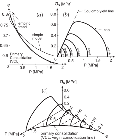
Figure 1: Granular yield surface, or jamming phase diagram, for $T_{g}=0$, as a function of the pressure $P$, shear stress $\sigma_{s}$, and void ratio $e\equiv\rho_{G}/\rho-1$. All thick solid lines are calculated using Eqs (43,51,54). (a): Maximal void ratio $e$ versus pressure $P$, or the virgin consolidation line. The dotted line is an empirical formula, $e=0.679-0.097\ln(P/0.5)$, with $P$ in Mpa. The thin line (designated as simple model) renders Eq (53). The circle at the top is the random loosest packing value for $e$. (b): The straight Coulomb yield line bends over depending on $e$, a behavior usually accounted for by the cap model in elasto-plastic theories. (c): The 3D combination of (a) and (b). Values for the calculation are : ${\cal B}_{0}=7000$ Mpa, $\rho_{\ell p}^{*}=0.445\rho_{G}$, $\rho_{cp}=0.645\rho_{G}$, $\Delta_{1}=10^{-4}$, and $k_{1}=10^{-5}$ m³/kg, $k_{2}=1000$, $k_{3}=0.01$.

First, a conceptual point. We take any yield surface as the divide between two regions: One in which stable elastic solutions are possible, the other in which they are not – so a system under stress must flow and cannot come to rest here. Accepting this, the natural approach is to have a convex elastic energy turn concave at the yield surface. The idea behind it is, the energy is an extremum if the equilibrium conditions of section III, including especially Eq (20), are met. Convexity implies the energy is at a minimum there, and concavity that it is at a maximum. Where $w_{1}$ is concave, any elastic solution satisfying Eq (20) has maximal energy, and is eager to get rid of it. It is not stable because infinitesimal perturbations suffice to destroy it.

As discussed in section II, for ${\cal B},\xi$= constant, $w_{1}$ is convex for $\pi_{s}/P\leq\sqrt{2/\xi}$ and concave otherwise, and already possesses the right form to account for the Coulomb yield line, see Fig 1-(b). Our task now is to appropriately generalize it such that the density $\rho$ is included as a third variable. Instead of $\rho$, the void ratio, $e\equiv\rho_{G}/\rho-1$, is frequently employed. It remains constant at elastic compressions and accounts for granular packaging only. ($\rho_{G}$ the bulk density of granular material, typically around $2700$ kg/m³ for sand.)

VI.2 Density Dependence of $\cal B$

We shall take ${\cal B}$ as density dependent, but not $\xi$: Since the Coulomb yield line is approximately independent of the density, so must the coefficient $\xi$ be, see Eq (4). Granular sound velocity was measured by Hardin and Richart Hardin , who found it linear in the void ratio, $c\sim 2.17-e$. Given Eq (43), the velocity of sound is $c\sim\sqrt{{\cal B}/\rho}$, implying

$${\cal B}={\cal B}_{0}(3.17-\rho_{G}/\rho)^{2}(\rho/\rho_{G}).$$ (49)

Since this expression properly accounts for the measured Kuwano density dependence of the compliance tensor $M_{ijk\ell}$, the dependence of $\cal B$ on $\rho$ seems settled SoilMech . It is not, because the resultant $w_{1}$ is concave in the variables $\rho$ and $\Delta$, and could not possibly sustain any static solution. Inserting Eq (49) into (43), we find the energy violating the stability condition,

$$\partial^{2}\mathcal{B}^{-2/3}/\partial\rho^{2}\leq 0,$$ (50)

obtained from inserting Eq (43) with $u_{s}\equiv 0$ into $(\partial^{2}w_{1}/\partial\rho^{2})\,(\partial^{2}w_{1}/\partial\Delta^{2})\geq(\partial^{2}w_{1}/\partial\rho\partial\Delta)^{2}$. Clearly, the widely employed Hardin-Richart relation, $c\sim 2.17-e$, is not accurate enough for a direct input into the energy. It works fine as long as the sand is jammed, $T_{g}=0$, and $\rho$ is only a given parameter, not a free variable – such as in the experiments of Kuwano , or when determining static stress distributions. But if a finite $T_{g}$ frees the density to become a variable, this instability will wreck havoc with the hydrodynamic theory. We need to reconstruct the density dependence of $\cal B$, such that the energy $w_{1}$

1. vanishes for densities smaller than the random loosest packing value (around the void ratio of $e_{\ell p}\approx 0.8$ for sand of uniform grain size), or $\rho\leq\rho_{\ell p}$;

2. (as a simplification) diverges at $\rho=\rho_{cp}$, the random closest packing value (around $e_{cp}\approx 0.55$);

3. is convex and reproduces the Hardin-Richart relation between $\rho_{\ell p}$ and $\rho_{cp}$.

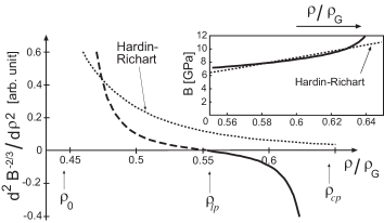
Figure 2: Equation (49), obtained by employing the Hardin-Richart relation directly, violates the stability condition Eq (50), because $\partial^{2}\mathcal{B}^{-2/3}/\partial\rho^{2}>0$ for all density values. Although numerically similar, see insert, the expression from Eq (51) suitably becomes concave at $\rho_{\ell c}$, and satisfies the stability condition between $\rho_{\ell c}$ and $\rho_{cp}$. The plots are calculated with $\rho_{\ell c}^{*}=0.445\rho_{G}$, $\rho_{pc}=0.645\rho_{G}$ (implying $\rho_{\ell p}=0.555\rho_{G}$), and ${\cal B}_{0}=7000$ Mpa, appropriate for Ham River sand Kuwano .

Alas, these points are more easily stated than combined in an energy expression, and no continuous $\cal B$ seems feasible: If analytic, $\cal B$ would be proportional to $\rho-\rho_{\ell p}$ close to $\rho_{\ell p}$. More generally, we may take ${\cal B}\sim(\rho-\rho_{\ell p})^{\alpha}$, with $\alpha$ positive. But the resulting energy, $w\sim(\rho-\rho_{\ell p})^{\alpha}\Delta^{2.5}$, remains concave. Only when including the divergence at $\rho_{cp}$ by taking ${\cal B}\sim(\rho-\rho_{\ell p})^{\alpha}/(\rho_{cp}-\rho)^{\beta}$ does the energy turn convex, between $\rho_{cp}$ and a density larger than $\rho_{\ell p}$. We therefore propose

$${\cal B} = {\cal B}_{0}\left(\frac{\rho-\rho^{*}_{\ell p}}{\rho_{cp}-\rho}\right)^{0.15}\times{\cal C},\quad\text{for}\,\,\rho>\rho_{\ell p};$$ (51)

$${\cal B} = 0,\qquad\qquad\qquad\qquad\quad\text{for}\,\,\rho\leq\rho_{\ell p}.$$ (52)

With an appropriate $\rho^{*}_{\ell p}<\rho_{\ell p}$, this expression renders the energy divergent at $\rho_{cp}$, stable and convex up to $\rho_{\ell p}$, and approximates the Hardin-Richart relation between them, see Fig. (2). (Take ${\cal C}=1$ for now, until it is specified otherwise in the next section.)

VI.3 Higher-Order Strain Terms

Next, we consider the unjamming transition in connection with compaction by pressure increase, the fact that denser sand can sustain more compression before getting unjammed, before elastic solutions become unstable: See the dotted line of Fig 1-(a), depicting a well-known empirical formula from soil mechanics elaPla-1 ; elaPla-2 ; elaPla-3 , $e=e_{0}-\Lambda\ln P$. Referred to as the virgin (or primary) consolidation line, it represents the boundary that sand (at rest) will not cross when compressed. Instead, it will collapse, becoming more compact, with a smaller $e$, close to or at the curve, but not beyond. (Note the dotted line does not appear to cut the $e$-axis, as it should at $\rho_{\ell p}$ – this is where sand becomes instable for any pressure. The discrepancy may derive from difficulties of making reliable measurements close to $\rho_{\ell p}$.)

This behavior is a natural consequence of higher-order strain terms such as the next order ones ($\zeta_{1},\zeta_{2}>0$),

$$-(\zeta_{1}\Delta^{3}+\zeta_{2}\Delta u_{s}^{2}),$$ (53)

which need to be added to $w_{1}$ as given by Eqs (43,51). Consider first pure compression, $u_{s}^{2}=0$. For small $\Delta$, the term $-\zeta_{1}\Delta^{3}$ is negligible, and $w_{1}$ remains convex. But if $\Delta$ is large enough, its negative second derivative will turn $w_{1}$ concave, making any elastic solution impossible. The value of $\Delta$ at which this happens, grows with $\cal B$ – a larger third-order term is needed for a larger $\cal B$. Now, $\cal B$ is smallest at $\rho=\rho_{\ell p}$, grows monotonically with $\rho$, and diverges at $\rho_{cp}$. As a result, the instability line cuts the $e$-axis at $\rho_{\ell p}$, veers towards larger $\Delta$ (or larger $P$) at higher density , and heads for infinity at $\rho_{cp}$, see the thin line depicted as “simple model” in Fig 1-(a), drawn with a constant $\zeta_{1}=24500$ MPa. (It is of course possible, employing a density-dependent $\zeta_{1}$, to improve the agreement to the dotted line.) In Fig 1-(b), the point of maximal pressure for a given void ratio $e$ is located at where the $P$-axis is being cut by the associated curve. If the term $\sim\Delta u_{s}^{2}$ did not exist, these curves would be vertical lines. The presence of $\sim\Delta u_{s}^{2}$ reduces the value of $\Delta$ (or $P$) for growing $u_{s}$ (or $\sigma_{s}$), bending the lines to the left.

Although qualitative figures of these curves that are frequently referred to as caps abound in textbooks elaPla-1 ; elaPla-2 ; elaPla-3 , we did not find enough quantitative data, especially not a generally accepted empirical expression, that we could have compared our results to. Presumably, it is not easy to observe caps in dry sand. Given this lack of reliable data, we decided against the expansion, Eq (53), and opted for a flexible “cap function,” $\cal C$ of Eq (51), capable of accounting for any possible cap-like unjamming transitions,

$$2{\cal C}=1+\tanh[(\Delta_{0}-\Delta)/\Delta_{1}],\quad\text{where}\quad$$ (54)

$$\Delta_{0}=k_{1}\rho-k_{2}u_{s}^{2}-k_{3}=k_{1}^{\prime}/(e+1)-k_{2}u_{s}^{2}-k_{3}.$$

With ${\cal C}\approx 1$ for $\Delta\ll\Delta_{0}$, and ${\cal C}\approx 0$ for $\Delta\gg\Delta_{0}$, the cap function is constructed to be relevant only in a narrow neighborhood around $\Delta_{0}$, for $|\Delta-\Delta_{0}|\lesssim\Delta_{1}\approx 10^{-4}$, such that the energy’s convexity is destroyed around $\Delta_{0}$. Taking $k_{1},k_{2},k_{3}$ as constant, $\Delta_{0}$ grows with the density and falls with $u_{s}^{2}$, giving rise to the typical appearance reproduced in Fig 1.

Together, Eqs (43,51,54) give the energy density $w_{1}$, appropriate for cohesionless granular materials at $T_{g}=0$. There are two contributions to the pressure, $P=P_{1}+P_{\Delta}$, where $P_{1}\equiv\rho(\partial w_{1}/\partial\rho)-w_{1}$ from Eq (48), and $\pi_{ij}=-\partial w_{1}/\partial u_{ij}\equiv P_{\Delta}\delta_{ij}-\sigma_{s}u_{ij}^{0}/u_{s}$. Because we still take $\Delta$ to be a small quantity, $P_{1}\sim\Delta^{2.5}$ may be neglected. (Similarly, terms such as $\pi_{ik}u_{jk}\sim\Delta^{2.5}$ from Eq (66) below are also negligible.) So the stress is simply $\pi_{ik}$, with pressure and shear stress given as

$$P_{\Delta} = {\cal B}\sqrt{\Delta}(\Delta+{\textstyle\frac{3}{10}}u_{s}^{2}/\Delta)-w_{1}{\cal C}^{*}/\Delta_{1},$$ (55)

$$\sigma_{s} = {\textstyle\frac{6}{5}}{\cal B}\sqrt{\Delta}u_{s}-2k_{2}u_{s}w_{1}{\cal C}^{*}/\Delta_{1},$$ (56)

where ${\cal C}^{*}\equiv 1-\tanh[(\Delta_{0}-\Delta)/\Delta_{1}]$, hence ${\cal C}^{*}\to 0$ away from the cap. (The terms of higher order in $\Delta$ are kept in ${\cal C}^{*}$, because $\Delta_{1}$ is small. This is how we make $\cal C$ a function relevant for $\Delta\approx\Delta_{0}$, not $\Delta\to 0$.)

Stability is given only if the energy $w_{1}$ is convex with respect to its seven variables, $\rho,\Delta,u_{ij}^{0}$. As linear transformations do not alter the convexity property of any function, we may take the energy as $w_{7}(\rho,\Delta,x_{1-5})$ where $x_{1}\equiv\sqrt{2}u_{xy}$, $x_{2}\equiv\sqrt{2}u_{xz}$, $x_{3}\equiv\sqrt{2}u_{yz}$, $x_{4}\equiv(u_{xx}-u_{zz})/\sqrt{2}$, $x_{5}\equiv(u_{xx}-2u_{yy}+u_{zz})/\sqrt{6}$. The characteristic polynomial $N_{7}$ of the Hessian matrix of $w_{7}$ is $N_{7}=(\lambda-u_{s}^{-1}\partial w_{1}/\partial u_{s})^{4}N_{3}$, with $N_{3}$ the characteristic polynomial of $w_{1}(\Delta,u_{s},\rho)$. Since $u_{s}^{-1}\partial w_{1}/\partial u_{s}$ is always positive, it is sufficient to consider $w_{1}(\Delta,u_{s},\rho)$. Requiring $N_{3}$ to have only positive eigenvalues defines the stable region in the strain space, spanned by $\Delta,u_{s},e$. Using Eqs (55,56), we may convert this into one in the stress space, spanned by $P,\sigma_{s},e$. The result, obtained numerically, is the yield surface plotted in Fig 1.

VI.4 Pressure Contribution From Agitated Grains

Agitated grains are known to exert a pressure in granular liquid. Using the model of ideal gas (better: non-interacting atoms with excluded volumes), with $w_{2}\sim{\rho T_{g}}$ denoting the energy density of agitated grains, the pressure expression,

$$P_{T}(\rho,T_{g})\sim{w_{2}}/({1-\rho/\rho_{cp}}),$$ (57)

was employed and found to account realistically for the behavior of granular liquid sandwiched between two cylinders rotating at different velocities Lub-1 ; Lub-2 ; Lub-3 ; Lub-4 .

In ideal gas, both the energy density $w$ and pressure $P$ are proportional to the temperature $T$. As a consequence, the entropy is $s\sim\ln T$, and diverges for $T\to 0$. (The free energy has a contribution $\sim T\ln T$ that vanishes for $T\to 0$.) As quantum effects become important long before $T$ vanishes, the unphysical feature of a diverging entropy is inconsequential for ideal gases. Yet this would be a highly relevant defect for granular solids, for which important physics occurs at or around $\bar{T}_{g}=0$. This is the reason ideal gas is not an appropriate model for granular solids. The considerations of section IV show that $w_{2},f_{2}\sim\bar{T}_{g}^{2}$ close to $\bar{T}_{g}=0$ – implying a pressure contribution, $P_{2}=\rho(\partial f_{2}/\partial\rho)-f_{2}\sim\bar{T}_{g}^{2}$, see Eq (48). Note first that $P_{2}\sim w_{2}$ is retained, and second that because $P_{0}=0$, $P_{1}\approx 0$, we have $P_{T}\equiv\sum P_{i}\approx P_{2}$.

Unfortunately, the density dependence of Eq (57) also poses a problem, as it implies a free energy $f_{2}=b_{0}\rho\ln(1-\rho/\rho_{cp})(-T_{g}^{2}/2)$ and a granular entropy, $s_{g}=-\partial f_{2}/\partial T_{g}=b_{0}\rho\ln(1-\rho/\rho_{cp})\,T_{g}$, both diverging for $\rho\to\rho_{cp}$. We therefore take $f_{2}$ to be given as in Eq (44), with a positive but small $a$. The resulting entropy is physically acceptable, and the pressure is easily rendered numerically indistinguishable from Eq (57),

$$P_{T} = P_{2}=\frac{\rho}{2\rho_{cp}}\frac{a\,\rho\,b_{0}\bar{T}_{g}^{2}}{(1-\rho/\rho_{cp})^{1-a}},$$ (58)

$$s_{g} = -\frac{\partial f_{2}}{\partial\bar{T}_{g}}=\rho\,b_{0}\bar{T}_{g}\left(1-\frac{\rho}{\rho_{cp}}\right)^{a}.$$ (59)

As the total pressure is now $P=P_{T}+P_{\Delta}$, cf. Eq (55), the jamming transition discussed above is modified. For instance, the yield condition of Eq (3), with $\xi=5/3$, now reads

$$\frac{\pi_{s}}{P_{\Delta}}=\frac{\pi_{s}}{P-P_{T}}\leq\sqrt{\frac{6}{5}},$$ (60)

implying a smaller maximal $\pi_{s}$ for given $P$. On the other hand, the maximal value for the void ratio $e$ is larger when $P_{T}$ is present: Any given $e$ has a maximal elastic compression $\Delta$ that will not sustain a larger $e$. But if $P$ is fixed and $T_{g}$ is finite, the elastic compression $\Delta$ will be appropriately smaller to sustain a larger $e$. This behavior is depicted in Fig 3.

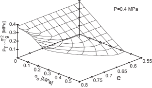
Figure 3: Jamming transition as a function of $e,\sigma_{s}$ and $P_{T}\sim T_{g}^{2}$, for $P_{\Delta}=0.4$ MPa. Values of model parameters are the same as those in FIG. 1.

The jamming transition, from elastic solid to liquid, is of course no longer completely sharp at a finite $T_{g}$, because $T_{g}$ turns the elastic body into a transiently elastic one for all values of stress and density. Nevertheless, there is a huge quantitative difference between catastrophic unjamming and the gradual process of stress relaxation. A sand pile may slowly degrade, relaxing toward the flat surface. But when turning on $T_{g}$ violates Eq (60), sudden events such as liquefaction happen. ($P_{T}$ may be substituted by the pore pressure to account for a similar collapse, if the soil is filled with water.) The frequently reported phenomenon of a primary earthquake emitting elastic waves that trigger earthquakes elsewhere Jia2 , may well be connected to Eq (60): $T_{g}$ as given by Eq (35) accompanies elastic waves. It may be sufficiently large to violate Eq (60) if stability was precarious.

VI.5 The Edwards Entropy

It is useful, with the free energy obtained in this chapter in mind, to revisit the starting points of Granular Statistical Mechanics (gsm), especially the Edwards entropy Edw . Taking the entropy $S(W,V)$ as a function of the energy $W$ and volume $V$, or ${\rm d}S=(1/T){\rm d}W+(P/T){\rm d}V$, it argues that a mechanically stable agglomerate of infinitely rigid grains at rest has, irrespective of its volume, vanishing energy, $W\equiv 0$, ${\rm d}W=0$. The physics is clear: However we package these rigid grains that neither attract nor repel each other, the energy remains zero. Therefore, ${\rm d}S=(P/T){\rm d}V$, or ${\rm d}V=(T/P){\rm d}S\equiv X{\rm d}S$. This is the starting expression of gsm, and $X$ is considered the relevant quantity characterizing granular media at rest. The entropy $S$ is obtained by counting the number of possibilities to package grains for a given volume, taking it to be $e^{S}$. And because a stable agglomerate is stuck in one single configuration, some tapping (or a similar disturbance) is taken to be needed to enable the system to explore the phase space.

In gsh, the grains are neither infinitely rigid, nor generally at rest. An elastic and a $T_{g}$-dependent energy contribution, denoted respectively as $f_{1}$ and $f_{2}$, see Eq (42), account for them. gsh also possesses a $T_{g}$-switch that determines whether the system’s behavior is solid- or liquid-like. This is clearly the generalization of phase space exploration enabled by tapping. That grains neither attract nor repel each other is accounted for by the stress vanishing for $T_{g},u_{ij}\to 0$: In this limit, in which $f_{1},f_{2}=0$ and only $f_{0}\sim\rho$ finite, there is no term in the energy that depends nonlinearly on the density $\rho$, hence $\sigma_{ij}=\partial(f_{0}/\rho)/\partial(1/\rho)\delta_{ij}=0$.

Given this comparison, it is natural to ask whether gsm is a legitimate limit of gsh. The answer is probably no, as both appear conceptually at odds in two points, the first more direct, the second quite fundamental: (1) Because of the Hertz-like contact between grains, very little material is being deformed at first contact, and the compressibility diverges at vanishing compression. This is a geometric fact independent of how rigid the bulk material is. Infinite rigidity is therefore not a realistic limit for sand. (2) In considering the entropy, one must not forget that the number of possibilities to package grains for a given volume is vastly overwhelmed by the much more numerous configurations of the inner granular degrees of freedom. Maximal entropy $S$ for given energy therefore realistically implies minimal macroscopic energy, such that a maximally possible amount of energy is in $S$ (or heat), equally distributed among the numerous inner granular degrees of freedom. Maximal number of possibilities to package grains for a given volume is a fairly different criterion.

VII Granular Hydrodynamic Theory

VII.1 Derivation

We take the conserved energy $w(s,s_{g},\rho,g_{i},u_{ij})$ of granular media to depend on entropy $s$, granular entropy $s_{g}$, density $\rho$, momentum density $g_{i}$, and the elastic strain $u_{ij}$. Defining the conjugate variables as $T\equiv\partial w/\partial s$, $\bar{T}_{g}\equiv T_{g}-T\equiv\partial w/\partial s_{g}$ [see Eq (23)], $\mu-v^{2}/2\equiv\partial w/\partial\rho$ [see Eq (8)], $v_{i}\equiv\partial w/\partial g_{i}=g_{i}/\rho$ [see Eq (5)], $\pi_{ij}\equiv-\partial w/\partial u_{ij}$, we write

$${\rm d}w=T{\rm d}s+\bar{T}_{g}{\rm d}s_{g}+(\mu-v^{2}/2){\rm d}\rho$$ (61)

$$+v_{i}{\rm d}g_{i}-\pi_{ij}{\rm d}u_{ij}.$$

The equations of motion for the energy and its variables are

$$\partial_{t}w+\nabla_{i}Q_{i}=0,\quad\partial_{t}\rho+\nabla_{i}(\rho v_{i})=0,\qquad$$ (62)

$$\partial_{t}g_{i}+\nabla_{j}(\sigma_{ij}+g_{i}v_{j})=0,\qquad\qquad$$ (63)

$$\partial_{t}s+\nabla_{i}f_{i}=R/T,\quad\!\!\partial_{t}s_{g}+\nabla_{i}F_{i}=R_{g}/T_{G},$$ (64)

$${\rm d}_{t}u_{ij}-v_{ij}-X_{ij}=\qquad\qquad\qquad\qquad$$ (65)

$$-[(u_{ik}\nabla_{j}v_{k}+\nabla_{i}y_{j}/2)+(i\leftrightarrow j)].$$

The first three equations are conservation laws, with the fluxes $Q_{i}$ and $\sigma_{ij}$ as yet unknown, to be determined in this section. The next two are the balance equation for the two entropies, the form of which are already given, in Eqs (30,32,33,34). Nevertheless, to see that they indeed fit the constraints required by energy and momentum conservation, we designate the currents as $f_{i}=sv_{i}-f_{i}^{D}$, $F_{i}=s_{g}v_{i}-F^{D}_{i}$, leaving $f_{i}^{D},F^{D}_{i},R,R_{g}$ unspecified. The last is the equation of motion for the elastic strain field, as discussed in section V, with $y_{i},X_{ij}$ the unknown fluxes to be determined here. Next, we introduce $\sigma^{D}_{ij}+\Sigma^{D}_{ij}$, as

$$\sigma_{ij}\equiv(-\tilde{f}+\mu\rho)\delta_{ij}-(\sigma^{D}_{ij}+\Sigma^{D}_{ij})$$ (66)

$$+\pi_{ij}-\pi_{ik}u_{jk}-\pi_{jk}u_{ik},$$

where $\tilde{f}\equiv w_{0}-Ts-\bar{T}_{g}s_{g}$, as in Eq (27,48). This is simply a definition of $\sigma^{D}_{ij}+\Sigma^{D}_{ij}$, which transfer our task from determining $\sigma_{ij}$ to finding the new quantity. This simplifies our task, notationally, of finding the form of $\sigma_{ij}$, it does not in anyway prejudice it.

Differentiating the energy, ${\partial_{t}}w=T{\partial_{t}}s+\bar{T}_{g}{\partial_{t}}s_{g}+(\mu-v^{2}/2){\partial_{t}}\rho+v_{i}{\partial_{t}}g_{i}-\pi_{ij}{\partial_{t}}u_{ij}$, see Eq (61), then inserting Eqs (62,63,64,65) into it, employing relations such as $\bar{T}_{g}\partial_{t}s_{g}=\bar{T}_{g}R_{g}/T_{G}+v_{k}s_{g}\nabla_{k}\bar{T}_{g}-\nabla_{k}(\bar{T}_{g}s_{g}v_{k})$, we obtain

$$\nabla_{i}Q_{i}=\nabla_{i}(Tf_{i}+\bar{T}_{g}F_{i}+\mu\rho v_{i}+v_{j}\sigma_{ij}-y_{j}\pi_{ij})\qquad$$ (67)

$$-R+f_{i}^{D}\nabla_{i}T+\sigma_{ij}^{D}v_{ij}+y_{i}\nabla_{j}\pi_{ij}+X_{ij}\pi_{ij}+\gamma\bar{T}_{g}^{2}$$

$$-R_{g}+\Sigma_{ij}^{D}v_{ij}+F_{i}^{D}\nabla_{i}\bar{T}_{g}-\gamma\bar{T}_{g}^{2}$$

This is a useful result, which shows one can rewrite ${\partial_{t}}w$ as the divergence of something (first line), plus something (second and third line) that vanishes in equilibrium – see section III.3 why $\nabla_{i}T,v_{ij},\pi_{ij},\nabla_{j}\pi_{ij}$ and $T_{G}$ vanish. We take the first line to yield the energy flux, $Q_{i}$, and the next two lines to vanish independently,

$$Q_{i} = Tf_{i}+\bar{T}_{g}F_{i}+\mu\rho v_{i}+v_{j}\sigma_{ij}-y_{j}\pi_{ij},$$ (68)

$$R = f_{i}^{D}\nabla_{i}T+\sigma_{ij}^{D}v_{ij}+y_{i}\nabla_{j}\pi_{ij}+X_{ij}\pi_{ij}+\gamma\bar{T}_{g}^{2},$$ (69)

$$R_{g} = \Sigma_{ij}^{D}v_{ij}+F_{i}^{D}\nabla_{i}\bar{T}_{g}-\gamma\bar{T}_{g}^{2}.$$ (70)

Comparing $R,R_{g}$ with Eqs (32,34), the currents are found as

$$f^{D}_{i}=\kappa\nabla_{i}T,\quad\sigma_{ij}^{D}=\zeta v_{\ell\ell}\delta_{ij}+\eta v^{0}_{ij}+\alpha\pi_{ij},$$ (71)

$$F^{D}_{i}=\kappa_{g}\nabla_{i}\bar{T}_{g},\quad\quad\Sigma_{ij}^{D}=\zeta_{g}v_{\ell\ell}\delta_{ij}+\eta_{g}v^{0}_{ij},$$

$$y_{i}=\beta^{P}\nabla_{j}\pi_{ij},\,\,X_{ij}=\beta\pi_{ij}^{0}+\beta_{1}\delta_{ij}\pi_{\ell\ell}-\alpha v_{ij}.$$

(It is an assumption to take $F_{i}^{D}\nabla_{i}\bar{T}_{g}$ as part of $R_{g}$ rather than $R$.) The two terms preceded by $\alpha$ contribute $\pm\alpha\pi_{ij}v_{ij}$ to $R$, respectively, hence cancel each other and are compatible with Eq (32). (More such pairs of terms, mutually canceling or contributing in equal parts, are possible. They have been excluded as a simplification. In the language of the Onsager force-flux relation, the above fluxes possess only diagonal elements, with the exception of the reactive, off-diagonal terms $\sim\alpha$.) Defining two relaxation times,

$$\frac{1}{\tau}\equiv 2\beta{\cal A}\sqrt{\Delta},\quad\frac{1}{\tau_{1}}\equiv 3\beta_{1}\sqrt{\Delta}\left({\cal B}+\frac{{\cal A}u_{s}^{2}}{2\Delta^{2}}\right).$$ (72)

the last of Eqs (71) may be written as

$$X_{ij}=\Delta\,\delta_{ij}/{\tau_{1}}-{u_{ij}^{0}}/\tau-\alpha v_{ij}.$$ (73)

To ensure permanent elasticity in granular statics, we must in addition require

$$X_{ij}\to 0\quad\text{for}\quad T_{g}\to 0.$$ (74)

This completes the derivation of gsh. Given $f_{i}^{D},F_{i}^{D},\sigma_{ij}^{D},\Sigma_{ij}^{D},y_{i},X_{ij}$, the structure of all currents in the set of equation, Eqs (62,63,64,65), are known. The question that remains is whether these expressions are unique. For simpler hydrodynamic theories, such as for isotropic liquid, nematic liquid crystal, or elastic solid, this procedure (frequently referred to as the standard procedure) is easily shown to be unique, because one can convince oneself that as long as the energy $w$ remains unspecified, there is only one way to write the time derivative of the energy $\partial_{t}w$ as the sum of a divergence and a series of expressions that vanish in equilibrium. In the present case, with two levels of entropy productions, one of which controls the switch between permanent and transient elasticity, the hydrodynamic theory is singularly intricate, and peripheral ambiguity remains. Nevertheless, displaying energy and momentum conservation explicitly, and reducing to liquid and solid hydrodynamics in the proper limits, the given set of equations is certainly a viable and consistent theory.

A more formal way of obtaining the fluxes of Eqs (71) is to define the flux and force vectors as $\vec{Z}=(f^{D}_{i},y_{i},\sigma^{D}_{ij},X_{ij})$, $\vec{Z}_{g}=(F^{D}_{i},\Sigma^{D}_{ij})$, $\vec{Y}=(\nabla_{i}T,\nabla_{j}\pi_{ij},v_{ij},\pi_{ij})$, $\vec{Y}_{g}=(\nabla_{i}\bar{T}_{g},v_{ij})$. And because $R=\vec{Z}\cdot\vec{Y}$, $R_{g}=\vec{Z}_{g}\cdot\vec{Y}_{g}$, the Onsager force-flux relations are given as

$$\vec{Z}=\hat{c}\cdot\vec{Y},\quad\vec{Z}_{g}=\hat{c}_{g}\cdot\vec{Y}_{g}.$$ (75)

The transport matrices, $\hat{c}$ and $\hat{c}_{g}$, have positive diagonal elements and off-diagonal ones that satisfy the Onsager reciprocity relation. Our example above has only diagonal elements, with the single exception of the reactive, off-diagonal terms $\sim\alpha$.

VII.2 Results

Collecting the terms derived above, in section VII.1, the equations of gsh, with $\sigma_{ij}$ valid to lowest order in strain, are

$$\partial_{t}\rho+\nabla_{i}(\rho v_{i})=0,\qquad\qquad\quad$$ (76)

$${\rm d}_{t}u_{ij}=(1-\alpha)v_{ij}-{u_{ij}^{0}}/\tau-{u_{\ell\ell}\,\delta_{ij}}/{\tau_{1}}\qquad$$

$$-(u_{ik}\nabla_{j}v_{k}+\nabla_{i}[\beta^{P}\nabla_{k}\pi_{jk}/2])-(i\leftrightarrow j),$$ (77)

$$\sigma_{ij}=(1-\alpha)\pi_{ij}-\pi_{ik}u_{jk}-\pi_{jk}u_{ik}\qquad\qquad\quad$$

$$+(\mu\rho-\tilde{f})\delta_{ij}-(\zeta+\zeta_{g})v_{\ell\ell}\delta_{ij}-(\eta+\eta_{g})v^{0}_{ij},$$ (78)

$$T_{g}[\partial_{t}s_{g}+\nabla_{i}(s_{g}v_{i}-\kappa_{g}\nabla_{i}\bar{T}_{g})]=R_{g}=\qquad\quad$$

$$\zeta_{g}v_{\ell\ell}^{2}+\eta_{g}v^{0}_{ij}v^{0}_{ij}+\kappa_{g}(\nabla_{i}\bar{T}_{g})^{2}-\gamma\bar{T}_{g}^{2},\,\,\,$$ (79)

$$T[\partial_{t}s+\nabla_{i}(sv_{i}-\kappa\nabla_{i}T)]=\zeta v_{\ell\ell}^{2}+\eta v^{0}_{ij}v^{0}_{ij}+\gamma\bar{T}_{g}^{2}$$

$$+\kappa(\nabla_{i}T)^{2}+\beta^{P}(\nabla_{j}\pi_{ij})^{2}+\beta\pi^{0}_{ij}\pi^{0}_{ij}+\beta_{1}\pi_{\ell\ell}^{2}.\,\,$$ (80)

Given in terms of the variables: ($s$, $s_{g}$, $\rho$, $g_{i}$, $u_{ij}$), conjugate variables ($T$, $\bar{T}_{g}$, $\mu$, $v_{i}$, $\pi_{ij}$), and 11 transport coefficients, ($\alpha$, $\tau$, $\tau_{1}$, $\zeta$, $\zeta_{g}$, $\eta$, $\eta_{g}$, $\gamma$, $\beta^{P}$, $\kappa$, $\kappa_{g}$), these equations are valid irrespective of the functional form of the energy $w$ and the transport coefficients. Therefore, they only provide a hydrodynamic structure, a framework into which different concrete theories fit. This circumstance, though also true for Newtonian fluids, is not as relevant there, because static susceptibilities (such as the compressibility or specific heat) and transport coefficients may frequently be approximated as constant. So the structure alone already possesses considerable predicting power. This is not true for granular media, which typically possess more involved functional dependence – especially concerning the $\bar{T}_{g}\to 0$ limit, which does not have a counter part in other systems. This is one of the less recognized reasons, we believe, underlying the complexity of granular systems.

In section VI, a free energy was proposed that we are confident should be fairly realistic. The situation with respect to the 11 transport coefficients are less settled, and in need of much future work, though a few limits are clear from the onset: First, a simple, analytic way to assure the elastic limit for $\bar{T}_{g}=0$ and satisfy the requirement of Eq (74) is given by

$$1/\tau=\lambda\bar{T}_{g},\quad 1/\tau_{1}=\lambda_{1}\bar{T}_{g},$$ (81)

which, as we shall see next, gives rise to the same dynamic structure as hypoplasticity. The density dependence is more subtle, hence harder and less urgent to determine. However, it seems plausible that $\lambda,\lambda_{1}$ should decrease for growing density, and especially the compressional relaxation should stop being operative at the random close packing density $\rho_{cp}$. To account for this, the simplest dependence would be

$$\lambda_{1}\sim(\rho-\rho_{cp}).$$ (82)

The coefficient $\alpha$ needs to vanish in the elastic limit, for $\bar{T}_{g}\to 0$, and be constant in the hypoplastic one, when $\bar{T}_{g}$ is moderately large: We have $\sigma_{ij}=\pi_{ij}$ in the elastic regime, and $\sigma_{ij}=(1-\alpha)\pi_{ij}+\cdots$ with $1-\alpha\approx 0.2$ in the hypoplastic one, implying sand is much softer here – same strain, yet stress is smaller by a factor of about five. The behavior of $\alpha$ is probably the result of granular agitation disrupting force chains. They are all intact in the elastic limit, making the system comparatively stiff. A finite $\bar{T}_{g}$ breaks up the chains, and when most of chains are destroyed, the remaining ones become essential in the sense that their disruption leads to local collapse, which in turn immediately repair the chains by some rearrangement. This is why $\alpha$ saturates and becomes constant.

Finally, as long as Eq (40) holds, the rate independence it entails would prevent the propagation of sound and elastic waves: Because both the elastic and the plastic part are linear in the velocity, and of the same order in the wave vector $q$, sound damping is comparable to sound velocity, and wave propagation could at most persist for a few periods. We therefore expand $\gamma,\eta_{g}$ in $\bar{T}_{g}$, as

$$\gamma=\gamma_{0}+\gamma_{1}\bar{T}_{g},\quad\eta_{g}=\eta_{1}\bar{T}_{g},$$ (83)

assuming $\eta_{g}$ lacks a constant term, because viscous dissipation occurs directly via $\eta$ for $\bar{T}_{g}\to 0$, see Eq (71). Inserting these expression into Eq (35) for a quick, qualitative estimate, we find $\bar{T}_{g}\sim{v_{ij}v_{ij}}\equiv v_{s}^{2}$ for $\gamma_{0}\gg\gamma_{1}\bar{T}_{g}$, and $\bar{T}_{g}\sim v_{s}$ for $\gamma_{0}\ll\gamma_{1}\bar{T}_{g}$. The first regime is essentially elastic, because the relaxation term, $u_{ij}/\tau\sim u_{ij}\bar{T}_{g}\sim u_{ij}v_{s}^{2}$, is of second order and small. This ensures the propagation of sound modes. In the second regime, the same term, $u_{ij}/\tau\sim u_{ij}\bar{T}_{g}\sim u_{ij}v_{s}$, is of first order and rather more prominent, giving rise to the hypoplastic behavior discussed in the next section .

VIII The Hypoplastic Regime

Hypoplasticity Kolym-1 , a modern, well-verified, yet comparatively simple theory of soil mechanics, models solid dynamics as realistically as the best of the elasto-plastic theories. Its starting point is the rate-independent constitutive relation,

$$\partial_{t}{\sigma}_{ij}=H_{ijk\ell}\,\,v_{k\ell}+\Lambda_{ij}\sqrt{v^{0}_{ij}v^{0}_{ij}+\epsilon\,v_{\ell\ell}^{2}},$$ (84)

where the coefficients $H_{ijk\ell},\Lambda_{ij},\epsilon$ are functions of $\sigma_{ij},\rho$, specified using experimental data mainly from triaxial apparatus. (Rate-independence means $\partial_{t}{\sigma}_{ij}$ is linearly proportional to the magnitude of the velocity, such that the change in stress remains the same for given displacement irrespective how fast the change is applied, a well verified observation in both the elastic and hypoplastic regime.) Great efforts are invested in finding accurate expressions for the coefficients, of which a recent set Kolym-1 is $\epsilon=1/3$,

$$H_{ijk\ell} = f\left(F^{2}\delta_{ik}\delta_{j\ell}+a^{2}\sigma_{ij}\sigma_{k\ell}/\sigma_{nn}^{2}\right)\text{,}$$ (85)

$$\Lambda_{ij} = aff_{d}F\left(\sigma_{ij}+\sigma_{ij}^{0}\right)/\sigma_{nn},$$ (86)

where $a=2.76$, $h_{s}=1600$ MPa,$\ e_{d}=0.44e_{i}$, $e_{c}=0.85e_{i}$, $e_{i}^{-1}=\exp\left(\sigma_{\ell\ell}/h_{s}\right)^{0.19}$, and

$$f_{d}=\left(\frac{e-e_{d}}{e_{c}-e_{d}}\right)^{0.25}\!\!\!\!\!\!,\quad f=-\frac{8.7h_{s}\left(1+e_{i}\right)}{3\left(\sigma_{s}/\sigma_{\ell\ell}+1\right)e}\left(\frac{\sigma_{\ell\ell}}{h_{s}}\right)^{0.81}\!\!\!\!\!\!,$$

$$F=\sqrt{\frac{3\sigma_{s}^{2}}{8\sigma_{\ell\ell}^{2}}+\frac{2\sigma_{s}^{2}\sigma_{\ell\ell}-3\sigma_{s}^{4}/\sigma_{\ell\ell}}{2\sigma_{s}^{2}\sigma_{\ell\ell}-6\sigma_{ij}^{0}\sigma_{j\ell}^{0}\sigma_{\ell i}^{0}}}-\sqrt{\frac{3}{8}}\frac{\sigma_{s}}{\sigma_{\ell\ell}}.$$

gsh, as derived above, reduces to Eq (84) for a stationary $T_{g}$, with $H_{ijlk},\Lambda_{ij},\epsilon$ given in terms of $M_{ijk\ell}\equiv-\partial^{2}w/\partial u_{ij}\partial u_{k\ell}$ and four scalars that are combinations of transport coefficients. We assume uniformity and stationarity, with especially $\nabla_{i}\bar{T}_{g},\nabla_{j}\pi_{ij},\partial_{t}v_{i}=0$, and only include the lowest order terms in the strain $u_{ij}$. We also take $\alpha,\eta_{g},\zeta_{g}$ as constants, and neglect $P_{T}$ from Eq (58), the pressure relevant in granular liquid, assuming $T_{g}$ is too small for the given velocity. It is then quite easy to evaluate $\partial_{t}\sigma_{ij}$ employing Eqs (77,78),

$${\partial_{t}}\sigma_{ij}=(1-\alpha){\partial_{t}}\pi_{ij}=(1-\alpha)M_{ijk\ell}{\partial_{t}}u_{k\ell}=$$

$${\textstyle(1-\alpha)M_{ijk\ell}[(1-\alpha)v_{k\ell}-u^{0}_{k\ell}/\tau-\delta_{k\ell}u_{mm}/{\tau_{1}}]}.$$ (87)

Clearly, given Eqs (35,81), this expression already has the structure of Eq (84) that Hypoplasticity postulates. And the coefficients are

$$H_{ijk\ell}=(1-\alpha)^{2}M_{ijk\ell},\qquad\epsilon=\zeta_{g}/\eta_{g},$$ (88)

$$\Lambda_{ij}=(1-\alpha)M_{ijk\ell}[(\tau/\tau_{1})\Delta\delta_{k\ell}-u_{k\ell}^{0}]\lambda{\sqrt{\eta_{g}/\gamma}}.$$ (89)

hpm has 43 free parameters (36+6+1 for $H_{ijk\ell},\Lambda_{ij},\epsilon$), all functions of the stress and density. Expressed as here, the stress and density dependence are essentially determined by $M_{ijk\ell}$ that is a known quantity ge-1 ; ge-2 . For the four free constants, we take

$$1-\alpha=0.22,\qquad\tau/{\tau_{1}}=0.09,$$ (90)

$$\frac{\zeta_{g}}{\eta_{g}}=0.33,\,\sqrt{\frac{\eta_{g}}{\gamma}}=\sqrt{\frac{\eta_{1}}{\gamma_{1}}}=\frac{114}{\lambda},$$

to be realistic choices, as these numbers yield satisfactory agreement with Hypoplasticity. Their significance are: $\zeta_{g}/\eta_{g}=0.33$ implies shear flows are three times as effective in creating $T_{g}$ as compressional flows. $\tau/\tau_{1}=0.09$ means, plausibly, that the relaxation rate of shear stress is ten times higher than that of pressure. The factor $(1-\alpha)^{2}$ accounts for an overall softening of the static compliance tensor $M_{ij\ell k}$. Finally, $\lambda$ controls the stress relaxation rate for given $T_{g}$, and ${\textstyle\sqrt{\eta_{1}/\gamma_{1}}}$ how well shear flow excites $T_{g}$. Together, $\lambda{\textstyle\sqrt{\eta_{g}/\gamma}}=114$ determines the relative weight of plastic versus reactive response: The term in Eq (84) preceded by $H_{ijk\ell}$ is the reversible, elastic response, the second term preceded by $\Lambda_{ij}$ comes from stress relaxation, is dissipative, irreversible and plastic. For small strain, $\Delta,u_{s}\to 0$, the elastic part is dominant, $|H_{ijk\ell}|\gg|\Lambda_{ij}|$. But $|\Lambda_{ij}|/|H_{ijk\ell}|\sim|u_{k\ell}^{0}|\cdot 114/(1-\alpha)$ is of order unity for $|u_{ij}|$ around $10^{-3}$.

Although the functions of Eqs (88,89) appear rather different from that of Eqs (85,86), the stress-strain increments are quite similar, as the comparison in JL3 shows. Moreover, the residual discrepancies may be eliminated by discarding the simplifying assumption of constant transport coefficients, independent of the stress. This agreement provides valuable insights into the physics of Hypoplasticity, showing why it works, what its range of validity is, and how it may be generalized. And it conversely also verifies gsh.

IX Conclusion

The success of Granular Elasticity, the theory we employ to account for static stress distribution in granular media, is mainly due to the fact that the information on the plastic strain is quite irrelevant there. This is no longer true in granular dynamics, when the system is being deformed – sheared, compressed or tapped. Starting from the working hypothesis that granular media are transiently elastic while being deformed, we aim to understand the notoriously complex plastic motion by combining two simple and transparent elements, elasticity and stress relaxation. In a recently published Letter JL3 , we proposed a model for granular solids based on this hypothesis. In the present manuscript, we give this model a consistent, hydrodynamic framework, compatible with conservation laws and thermodynamics.

The framework is valid for any healthy energy, but is essentially devoid of predictive power if the energy is left unspecified. Therefore, an explicit expression for the total, conserved energy is given. Encapsulating the key features of static granular media: stress distribution, incremental stress-strain relation, minimal and maximal density, the virgin consolidation line, the Coulomb yield line and the cap model, this expression should prove realistic enough for rendering the specific hydrodynamic theory useful. Much future work is needed to see whether further agreement between theory and experiments may be achieved, especially concerning cyclic loading, tapping and shear band.

Appendix A Equilibrium Conditions

First, noting $\pi_{ij}{\rm d}u_{ij}=\pi_{ij}{\rm d}\nabla_{j}U_{i}$ because $\pi_{ij}$ is symmetric, we write the energy density per unit volume (dropping the subscript of $w_{0}$ in this section) as

$${\rm d}w=T{\rm d}s+\mu{\rm d}\rho-\pi_{ij}{\rm d}\nabla_{j}U_{i}.$$ (91)

Next, we vary the energy $\int w{\rm d}V$ for given entropy $\int s{\rm d}V$, mass $\int\rho{\rm d}V$, and for fixed displacement at the medium’s surface, $\delta U_{i}=0$. Taking $\ell_{1},\ell_{2}$ as constant Lagrange parameters and denoting the surface element as ${\rm d}A_{i}$, we require the variation of the energy to be extremal,

$$\delta\int\left(w-\ell_{1}s-\ell_{2}\rho\right)\,{\rm d}V=0.$$ (92)

Inserting Eq (91) into (92), we find

$$\int\left[{T}\delta s+\mu\delta\rho+{\pi_{ij}}\delta\nabla_{j}U_{i}-\ell_{1}\delta s-\ell_{2}\delta\rho\right]\,{\rm d}V=$$

$$\int\left[\left({T}-\ell_{1}\right)\delta s+\left(\mu-\ell_{2}\right)\delta\rho-\left(\nabla_{j}{\pi_{ij}}\right)\delta U_{i}\right]\,{\rm d}V$$

$$\qquad+\oint{\pi_{ij}}\delta U_{i}\,{\rm d}A_{i}=0,$$

where the last term vanishes because $\delta U_{i}\equiv 0$ at the surface. If $\delta s$, $\delta\rho$ and $\delta U_{j}$ vary independently, all three brackets must vanish. And because $\ell_{1},\ell_{2}$ are constant, $T,\mu$ also need to be. So the conditions for the energy (or entropy) being extremal are

$$\nabla_{i}T=0,\quad\nabla_{i}\mu=0,\quad\nabla_{j}\pi_{ij}=0.$$ (93)

In granular media for $\bar{T}_{g}=0$, density and compression are coupled as

$${\rm d}u_{\ell\ell}=-{\rm d}\rho/\rho=\rho{\rm d}v,$$ (94)

and do not vary independently. Simply inserting this relation into the above calculation, we find $\nabla_{i}(\mu+\pi_{\ell\ell}/3\rho)=0$ to replace the last two conditions of Eq (93). This is not the correct result, because we have been varying the energy and its variables above, keeping the volume unchanged throughout, with $\delta U_{i}\equiv 0$ at the surface. But then $u_{\ell\ell}$ is fixed and cannot change with the density $\rho$: Consider a one-dimensional medium between $x=0$ and $x=x_{0}$, with $U_{x}(0),U_{x}(x_{0})$ given. Since $\nabla_{j}\pi_{ij}\sim\partial^{2}_{x}[U_{x}(x_{0})-U_{x}(0)]=0$, the one-dimensional strain is $u_{\ell\ell}=\partial_{x}U_{x}=(U_{x}(x_{0})-U_{x}(0))/x_{0}$ and cannot change.

To find the proper expression, we may take mass $M$ rather than volume $V$ as the constant quantity, and vary the density by changing the volume, or the length in the one-dimensional case. Holding $\delta U_{i}\equiv 0$ at the moving surface will then allow Eq (94) to hold. Denoting the energy, entropy and volume per unit mass, respectively, as $e\equiv w/\rho$, $\sigma\equiv s/\rho$, $v\equiv V/M=1/\rho$, and $f\equiv w-Ts$, the equivalent expression,

$${\rm d}e = T{\rm d}\sigma-P_{T}{\rm d}v-(\pi_{ij}/\rho){\rm d}\nabla_{j}U_{i},$$ (95)

$$P_{T} \equiv -w+Ts+\mu\rho=-f+\mu\rho,$$ (96)

holds. Now we have $E=\int e{\rm d}M$, $S=\int\sigma{\rm d}M$, $V=\int v{\rm d}M$, where ${\rm d}M=\rho{\rm d}V$ is the integrating mass element. Varying the energy for given entropy, volume and requiring it to vanish, $\delta E-\ell_{1}S-\ell_{2}V=0$, we find

$$\int\left[\left({T}-\ell_{1}\right)\delta\sigma+\left(P_{T}-\ell_{2}\right)\delta v\right]\,{\rm d}M=\int\left(\nabla_{j}{\pi_{ij}}\right)\delta U_{i}\,{\rm d}V.$$

implying $\nabla_{i}T=0$, $\nabla_{i}P_{T}=0$, and $\nabla_{j}\pi_{ij}=0$. These are the same conditions as Eq (93), because $\nabla_{i}P_{T}=s\nabla_{i}T+\rho\nabla_{i}\mu$. But if Eq (94) is implemented, turning Eq (95) to

$${\rm d}e = T{\rm d}\sigma-(P_{T}+\pi_{\ell\ell}/3){\rm d}v-(\pi^{0}_{ij}/\rho){\rm d}\nabla_{j}U_{i},$$ (97)

$$= T{\rm d}\sigma-\rho^{-1}(P_{T}\,\delta_{ij}+\pi_{ij})\,{\rm d}\nabla_{j}U_{i},$$ (98)

the equilibrium conditions are altered to become

$$\nabla_{i}T=0,\quad\nabla_{i}(P_{T}+\pi_{\ell\ell}/3)=0,\quad\nabla_{j}\pi^{0}_{ij}=0.$$ (99)

Clearly, the Cauchy, or total, stress in equilibrium is given as

$$\sigma_{ij}=P_{T}\delta_{ij}+\pi_{ij},\,\,\text{with}\,\,\nabla_{j}\sigma_{ij}=0.$$ (100)

Including the gravitational energy $\rho\phi$ in $w$, with $-\nabla_{i}\phi=G_{i}$, the gravitational constant pointing downward, we have

$${\rm d}w=T{\rm d}s+(\mu+\phi){\rm d}\rho-\pi_{ij}{\rm d}\nabla_{j}U_{i}+\rho\,{\rm d}\phi,$$ (101)

and find (via the same calculation as above) that $\mu+\phi$ is now a constant, implying an alteration of the second of Eqs (93) to

$$\nabla_{i}\mu=G_{i},$$ (102)

or equivalently, $\nabla_{i}P_{T}=s\nabla_{i}T+\rho\nabla_{i}\mu=\rho G_{i}$. If Eq (94) holds, $\nabla_{j}\sigma_{ij}=0$ is analogously changed to

$$\nabla_{j}\sigma_{ij}=\nabla_{j}(P_{T}\delta_{ij}+\pi_{ij})=\rho G_{i}.$$ (103)

References

- (1) H.M. Jaeger, S.R. Nagel, R.P. Behringer, Granular solids, liquids, and gases, Rev. Mod. Phys. 68, No. 4, 1259 (1996).
- (2) A.J. Liu and S.R. Nagel, Jamming is not just cool any more, Nature 396, 21 (1998).
- (3) P.G. de Gennes, Granular matter: a tentative view, Rev. Mod. Phys. 71, No. 2, 347 (1999).
- (4) L.P. Kadanoff, Built upon sand: Theoretical ideas inspired by the flow of granular materials, Rev. Mod. Phys. 71, No. 1, 435 (1999).
- (5) P. K. Haff, Grain flow as a fluid-mechanical phenomenon, J. Fluid Mech. 134, 401(1983).
- (6) J. T. Jenkins and S. B. Savage, A theory for the rapid flow of identical, smooth, nearly elastic particles, J. Fluid Mech. 130, 187(1983).
- (7) C.S. Campbell, Rapid Granular Flows, Ann. Rev. Fluid Mech. 22, 57 (1990).
- (8) H.J. Herrmann, J.-P. Hovi, S. Luding (Editors), Physics of Dry Granular Media, (Kluwer Academic Publishers, Dordrecht, 1998).
- (9) I. Goldhirsch, Chaos 9, 659 (1999).
- (10) A. Mehte, Granular Physics (Cambridge University Press, Cambridge, 2007).
- (11) L.E. Silbert, D. Ertas, G.S. Grest, T.C. Halsey, D. Levine, S.J. Plimpton, Granular flow down an inclined plane: Bagnold scaling and rheology, Phys. Rev. E 64, 051302 (2001).
- (12) GDR MiDi, On dense granular flows, Eur. Phys. J. E 14, 341 (2004).
- (13) P.Jop, Y. Forterre, O. Pouliquen, A constitutive law for dense granular flows, Nature 441, 727, 2006.
- (14) F. Alonso-Marroquin and H. J. Herrmann, Calculation of the incremental stress-strain relation of a polygonal packing, Phys. Rev. E 66, 021301(2002).
- (15) F. Alonso-Marroquin and H. J. Herrmann, Ratcheting of Granular Materials, Phys. Rev. Lett. 92, 054301(2004).
- (16) R. Garcia-Rojo, F. Alonso-Marroquin, H. J. Herrmann, Characterization of the material response in granular ratcheting, Phys. Rev. E 72, 041302(2005).
- (17) R.M. Nedderman, Statics and Kinematics of Granular Materials (Cambridge University Press, Cambridge, 1992).
- (18) A. Schofield, P. Wroth, Critical State Soil Mechanics (McGraw-Hill, London, 1968).
- (19) Engineering Properties of Soil edited by W.X. Huang (Hydroelectricity Publishing, Beijing, 1983) (in Chinese), 1st ed.
- (20) D. Kolymbas, Introduction to Hypoplasticity, (Balkema, Rotterdam, 2000).
- (21) D. Kolymbas, also W. Wu and D. Kolymbas, in Constitutive Modelling of Granular Materials ed D. Kolymbas, (Springer, Berlin, 2000), and references therein.
- (22) C. Truesdell and W. Noll, The nonlinear field theories of mechanics, Handbuch der Physik III/c, (Springer, Berlin, 1965).
- (23) C. Truesdell, Continuum Mechanics (Gordon and Breach, New York, 1965), Vols. 1 and 2.
- (24) L. D. Landau and E. M. Lifshitz, Fluid Mechanics (Butterworth-Heinemann, Oxford, 1987) and Theory of Elasticity (Butterworth-Heinemann, Oxford, 1986)
- (25) I.M. Khalatnikov, Introduction to the Theory of Superfuidity, (Benjamin, New York 1965).
- (26) S. R. de Groot and P. Masur, Non-Equilibrium Thermodynamics, (Dover, New York 1984).
- (27) D. Forster, Hydrodynamic Fluctuations, Broken Symmetry and Correlation Functions (Benjamin, New York, 1975).
- (28) P.G. de Gennes and J. Prost, The Physics of Liquid Crystals (Clarendon Press, Oxford 1993).
- (29) P.C. Martin, O. Parodi, and P.S. Pershan, Unified Hydrodynamic Theory for Crystals, Liquid Crystals, and Normal Fluids, Phys. Rev. A 6, 2401 (1972).
- (30) T.C. Lubensky, Hydrodynamics of Cholesteric Liquid Crystals, Phys. Rev. A 6, 452 (1972).
- (31) M. Liu, Hydrodynamic Theory near the Nematic Smectic-A Transition, Phys. Rev. A 19, 2090 (1979);
- (32) M. Liu, Hydrodynamic theory of biaxial nematics, Phys. Rev. A 24, 2720 (1981).
- (33) M. Liu, Maxwell equations in nematic liquid crystals, Phys. Rev. E 50, 2925, (1994).
- (34) H. Pleiner and H.R. Brand, in Pattern Formation in Liquid Crystals, edited by A. Buka and L. Kramer (Springer, New York, 1996).
- (35) R. Graham, Hydrodynamics of 3He in Anisotropic A Phase, Phys. Rev. Lett. 33, 1431 (1974).
- (36) R. Graham and H. Pleiner, Spin Hydrodynamics of 3He in the Anisotropic A Phase, Phys. Rev. Lett. 34, 792 (1975).
- (37) M. Liu, Hydrodynamics of 3He near the A-Transition, Phys. Rev. Lett. 35, 1577 (1975).
- (38) M. Liu and M.C. Cross, Broken Spin-Orbit Symmetry in Superfluid 3He and the B-Phase Dynamics, Phys. Rev. Lett. 41, 250 (1978).
- (39) Gauge Wheel of Superfluid 3He, Phys. Rev. Lett. 43, 296 (1979).
- (40) M. Liu, Relative Broken Symmetry and the Dynamics of the -Phase, Phys. Rev. Lett. 43, 1740 (1979).
- (41) M. Liu, Rotating Superconductors and the Frame-independent London Equations, Phys. Rev. Lett. 81, 3223, (1998).
- (42) Jiang Y.M. and M. Liu, Rotating Superconductors and the London Moment: Thermodynamics versus Microscopics, Phys. Rev. B 6, 184506, (2001).
- (43) M. Liu, Superconducting Hydrodynamics and the Higgs Analogy, J. Low Temp. Phys. 126, 911, (2002)
- (44) K. Henjes and M. Liu, Hydrodynamics of Polarizable Liquids, Ann. Phys. 223, 243 (1993).
- (45) M. Liu, Hydrodynamic Theory of Electromagnetic Fields in Continuous Media, Phys. Rev. Lett. 70, 3580 (1993).
- (46) Mario Liu replies, Phys. Rev. Lett. 74, 1884, (1995).
- (47) Y.M. Jiang and M. Liu, Dynamics of Dispersive and Nonlinear Media, Phys. Rev. Lett. 77, 1043, (1996).
- (48) M.I. Shliomis, Sov. Phys. Usp. 17, 153 (1974).
- (49) R.E. Rosensweig, Ferrohydrodynamics, (Dover, New York 1997).
- (50) M. Liu, Fluiddynamics of Colloidal Magnetic and Electric Liquid, Phys. Rev. Lett. 74, 4535 (1995).
- (51) M. Liu, Off-Equilibrium, Static Fields in Dielectric Ferrofluids, Phys. Rev. Lett. 80, 2937, (1998).
- (52) M. Liu, Electromagnetic Fields in Ferrofluids, Phys. Rev. E 59, 3669, (1999).
- (53) H.W. Müller and M. Liu, Structure of Ferro-Fluiddynamics, Phys. Rev. E 64, 061405 (2001).
- (54) H.W. Müller and M. Liu, Shear Excited Sound in Magnetic Fluid, Phys. Rev. Lett. 89, 67201, (2002).
- (55) O. Müller, D. Hahn and M. Liu, Non-Newtonian behaviour in ferrofluids and magnetization relaxation, J. Phys.: Condens. Matter 18, 2623, (2006).
- (56) S. Mahle, P. Ilg and M. Liu, Hydrodynamic theory of polydisperse chain-forming ferrofluids, Phys. Rev. E 77, 016305 (2008).
- (57) H. Temmen, H. Pleiner, M. Liu and H.R. Brand, Convective Nonlinearity in Non-Newtonian Fluids, Phys. Rev. Lett. 84, 3228 (2000).
- (58) H. Temmen, H. Pleiner, M. Liu and H.R. Brand, Temmen et al. reply, Phys. Rev. Lett. 86, 745 (2001).
- (59) H. Pleiner, M. Liu and H.R. Brand, Nonlinear Fluid Dynamics Description of non-Newtonian Fluids, Rheologica Acta 43, 502 (2004).
- (60) O. Müller, PhD Thesis University Tübingen (2006).
- (61) Y.M. Jiang, M. Liu, Granular Elasticity without the Coulomb Condition, Phys. Rev. Lett. 91, 144301 (2003).
- (62) Y.M. Jiang, M. Liu, Energy Instability Unjams Sand and Suspension, Phys. Rev. Lett. 93, 148001(2004).
- (63) Y.M. Jiang, M. Liu, A Brief Review of “Granular Elasticity”, Eur. Phys. J. E 22, 255 (2007).
- (64) D.O. Krimer, M. Pfitzner, K. Bräuer, Y. Jiang, M. Liu, Granular Elasticity: General Considerations and the Stress Dip in Sand Piles, Phys. Rev. E74, 061310 (2006).
- (65) K. Bräuer, M. Pfitzner, D.O. Krimer, M. Mayer, Y. Jiang, M. Liu, Granular Elasticity: Stress Distributions in Silos and under Point Loads, Phys. Rev. E74, 061311 (2006);
- (66) Y.M. Jiang, M. Liu, From Elasticity to Hypoplasticity: Dynamics of Granular Solids, Phys. Rev. Lett. 99, 105501 (2007).
- (67) see I.K. Ono, C.S. O Hern, D.J. Durian, S.A. Langer, A.J. Liu, S.R. Nagel, Phys. Rev. Lett. 89, 095703 (2002) and references therein.
- (68) P. Kostädt and M. Liu, Three ignored Densities, Frame-independent Thermodynamics, and Broken Galilean Symmetry,, Phys. Rev. E 58, 5535, (1998).
- (69) M. Liu, Comment on “Weakly and Strongly Consistent Formulation of Irreversible Processes”, Phys. Rev. Lett. 100, 098901 (2008)
- (70) P.G. de Gennes Superconductivity of Metals and Alloys, Addison-Wesley, New York (1992)
- (71) G.Y. Onoda and E.G. Liniger, Random loose packings of uniform spheres and the dilatancy onset, Phys. Rev. Lett., 64, 2727(1990).
- (72) B.O. Hardin and F.E. Richart, Elastic wave velocities in granular soils, J. Soil Mech. Found. Div. ASCE 89: SM1, pp 33-65(1963).
- (73) R. Kuwano and R.J. Jardine, On the applicability of cross-anisotropic elasticity to granular materials at very small strains, Geotechnique 52, 727 (2002).
- (74) Y.M. Jiang, M. Liu, Incremental stress-strain relation from granular elasticity: Comparison to experiments, Phys. Rev. E 77, 021306 (2008).
- (75) L. Bocquet, J. Errami, and T. C. Lubensky, Hydrodynamic Model for a Dynamical Jammed-to-Flowing Transition in Gravity Driven Granular Media, Phys. Rev. Lett., 89, 184301 (2002).
- (76) W. Losert, L. Bocquet, T. C. Lubensky, and J. P. Gollub, Particle Dynamics in Sheared Granular Matter, Phys. Rev. Lett., 85, 1428 (2000);
- (77) L. Bocquet, W. Losert, D. Schalk, T. C. Lubensky, and J. P. Gollub, Granular shear flow dynamics and forces: Experiment and continuum theory, Phys. Rev., E 65, 011307 (2002);
- (78) I. Goldhirsch, Rapid Granular Flows, Annu. Rev. Fluid Mech., 35, 267 (2003).
- (79) P.A. Johnson, X. Jia, Nonlinear dynamics, granular media and dynamic earthquake triggering Nature, 437/6, 871 (2005).
- (80) S.F. Edwards, R.B.S. Oakeshott, Theory of powders, Physica A 157, 1080 (1989); S.F. Edwards, D.V. Grinev, Statistical Mechanics of Granular Materials: Stress Propagation and Distribution of Contact Forces, Granular Matter, 4, 147 (2003).