Fe K$\alpha$ and hydrodynamic loop model diagnostics for a large flare on II Peg

Abstract

The observation by the Swift X-ray Telescope of the Fe K$\alpha_{1},\alpha_{2}$ doublet during a large flare on the RS CVn binary system II Peg represents one of only two firm detections to date of photospheric Fe K$\alpha$ from a star other than our Sun. We present models of the Fe K$\alpha$ equivalent widths reported in the literature for the II Peg observations and show that they are most probably due to fluorescence following inner shell photoionisation of quasi-neutral Fe by the flare X-rays. Our models constrain the maximum height of flare the to 0.15 R_∗ assuming solar abundances for the photospheric material, and 0.1 R_∗ and 0.06 R_∗ assuming depleted photospheric abundances ([M/H] = -0.2 and [M/H] = -0.4, respectively). Accounting for an extended loop geometry has the effect of increasing the estimated flare heights by a factor of $\sim$3. These predictions are consistent with those derived using results of flaring loop models, which are also used to estimate the flaring loop properties and energetics. From loop models we estimate a flare loop height of 0.13 R_∗, plasma density of $\sim 4\times 10^{12}$ cm^-3 and emitting volume of $\sim 6\times 10^{30}$ cm³. Our estimates for the flare dimensions and density allow us to estimate the conductive energy losses to $E_{cond}\leq 2\times 10^{36}$ erg, consistent with upper limits previously obtained in the literature. Finally, we estimate the average energy output of this large flare to be $\sim 10^{33}$ erg sec^-1, or 1/10th of the stellar bolometric luminosity.

1. Introduction

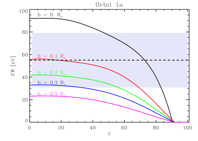
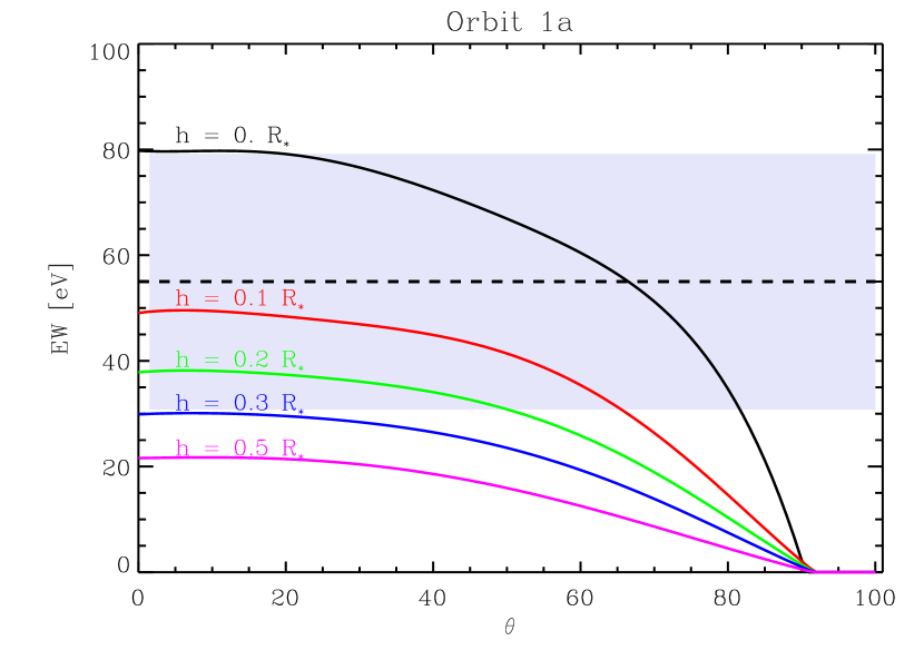
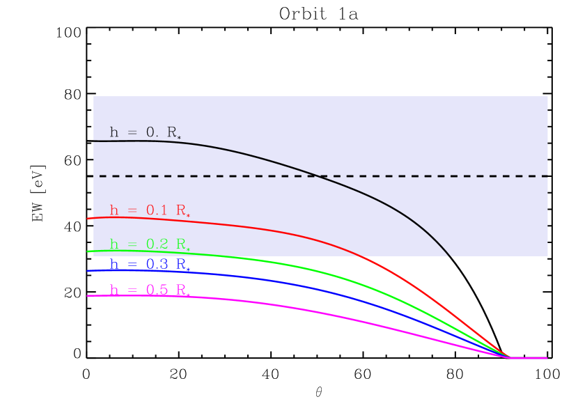
Figure 1.— Example Fe K$\alpha$ equivalent widths as a function of flare height and inclination angle for three different photospheric metallicities for the 1a segment of the flare, as defined by O07. The observed value and its error is indicated by the horizontal black dashed line and teh shaded area. Left: Models calculated at solar abundances (Grevesse & Sauval, 1998); Central: Models calculated with [M/H] = -0.2; Right: Models calculated with [M/H] = -0.4.

A fraction of the X-rays emitted during stellar flares or by hot stellar coronae are directed downwards towards the stellar photosphere. Here they interact with the photospheric gas and are reprocessed through scattering and photoionisation events. The downward cascade following inner shell photoionisation of quasi-neutral gas in the stellar photosphere produces characteristic fluorescent emission from astrophysically abundant species. While the reprocessed X-ray spectra reach the observer at low flux levels compared to that of the flares/coronae, fluorescent emission lines, can be significantly stronger and can be detected against the spectra of the flare/corona itself.

The intensity or equivalent width of the fluorescent lines detected at Earth depends uniquely on the details of the fluorescing spectrum, the photospheric abundance of the photoionised species and the geometry of the system (flare height and inclination angle; e.g. see fig. 2 of Testa et al., 2008), making them potentially powerful diagnostics. A number of theoretical studies exist which provide a framework for the interpretation of the strong iron fluorescent emission in the solar context (e.g. Tomblin, 1972; Bai, 1979), and more recently for arbitrarily photoionised slabs (Kallman et al., 2004) and stellar photospheres (Drake, Ercolano and Swartz, 2008, DES08). Drake & Ercolano (2008a,b) have also recently showed that fluorescent emission from neon and oxygen should also be detectable in the solar spectrum with current and future instrumentation. These may provide an independent measure of the photospheric solar oxygen and neon abundance, elements that are central to the solution of the “solar oxygen crisis” (e.g. Ayres et al. 2006, Socas-Navarro 2007, Basu & Antia 2008).

Observationally, the $2s-1p$ 6.4 KeV Fe K$\alpha$ doublet from low ionisation stages of iron has often been detected in solar spectra (e.g. Neupert et al., 1967; Doschek et al., 1971; Fedelman et al., 1980; Tanaka et al., 1984; Parmar et al. 1984; Zarro et al., 1992), from disks around pre-main sequence stars (e.g. Tsujimoto et al., 2005; Favata et al., 2005), and from the photospheres of the single G-type giant HR 9024 (Testa et al., 2007) and of the RS CVn binary system II Peg (Osten et al., 2007, hereafter O07).

The detection of the 6.4 keV fluorescent iron line in the Swift X-ray Telescope spectrum of II Peg taken during a large flare (O07) is particularly interesting as it represents the first of only two detections (with HR 9024, Testa et al., 2007) of photospheric fluorescence emission in stars other than the Sun. O07, however, assigned the excitation mechanism to electron impact ionization of photospheric Fe, rather than photoionisation. In this paper we show by means of Monte Carlo fluorescence modeling that the Fe K$\alpha$ equivalent widths reported by O07 are perfectly consistent with photoionisation induced fluorescence. We also show that our predictions of the flaring loop scale height agree with those from flaring loop models (Reale, 2007) and discuss other implications on flaring plasma density, volume and energetics.

In Section 2 we briefly describe our Monte Carlo model, and in Section 3 we present and discuss our results. Section 4 deals with the flaring loop properties and energetics from hydrodynamic models. Our final conclusions are given in Section 5.

2. Monte Carlo Fluorescence Calculations

The 3D Monte Carlo calculations presented here were performed using a modified version of the photoionisation and dust radiative transfer code, MOCASSIN (Ercolano et al. 2003, 2005, 2008). The code uses a a stochastic approach to the radiation transfer allowing it to deal with problems of arbitrary geometry, while treating both the primary and secondary components of the radiation field self-consistently. The modified version used in this work, which can deal with the production and transfer of fluorescent radiation, is further described by DES08.

We performed calculations to fit all Fe K$\alpha$ detections reported by O07 for the 5 different orbits (flare intervals) of the Swift X-ray telescope. Spectra representing the flaring source of X-ray irradiation for input into the photospheric fluorescence modeling were computed for each of these flare intervals. Spectra were computed using the CHIANTI database version 5.2 (Dere et al. 1997, Landi et al. 2006) for the energy range 6.2-30 keV, using the temperatures and emission measures found by O07 from two-temperature model fitting and listed in Table 3 of that article. The upper limit to the energy range was chosen to be sufficiently high that any contribution to the observed fluorescent Fe K line from higher energy photons in these thermal spectra should be less than 1%.

Photospheric metal abundances in II Peg have been studied by Ottmann et al. (1998) and Berdyugina et al. (1998). Both are based on high resolution, high signal-to-noise spectroscopy, and there is little to choose between the analyses. The former obtained abundances [Fe/H] $=-0.2$, [Mg/H] $=-0.15$, and [Si/H] $=-0.15$, expressed relative to the solar composition in conventional spectroscopic logarithmic bracket notation, and each with uncertainty of $\pm 0.1$. As a verification of their method, they successfully recovered the currently accepted solar atmospheric parameters from a spectrum of moonlight. Berdyugina et al. (1998) obtained [M/H] $=-0.4\pm 0.1$, and verified their approach against the detailed analysis of the K0 giant Pollux by Drake & Smith (1991). It is therefore reasonable to infer that II Peg is mildly metal-poor by 0.1-0.4 dex relative to the Sun. We have investigated the effects of this slight metal depletion on Fe K$\alpha$ equivalent widths by running three sets of models: (i) with solar abundances (Grevesse & Sauval, 1998), (ii) with [M/H] $=-0.2$ and (iii) with [M/H]$=-0.4$.

Fe K$\alpha$ equivalent widths also strongly depend on the geometry of the system, i.e. height of the flare, $h$, and inclination angle, $\theta$. In particular Fe K$\alpha$ efficiencies (and therefore equivalent widths) depend on the function $f(h,\theta)$, which has been numerically determined for the case of a single flare illuminating a spherical photosphere by DES08. Assuming that the flare can be approximated by a point source above the stellar surface, we have performed calculations at $h~{}=~{}0.,0.1,0.2,0.3,0.5$ and $\theta=0.$ and used the analytical form of $f(\theta)$ given by DES08 in order to estimate the inclination angle dependence. We note that in order to scale $\theta=0$ equivalent widths to an arbitrary value of $\theta$ using the $f(\theta)$ functions one has to first scale the latter such that $f(0)~{}=~{}1$.

3. Results from Monte Carlo Fluorescence Modeling

3.1. Assuming a point source flare

Representative flare geometry diagnostic diagrams illustrating the Fe K$\alpha$ line equivalent width as a function of $\theta$ for different flare heights are presented in Figure 1 for the three values of [M/H] (0.0, $-0.2$ and $-0.4$) for Orbit segment 1a. Also indicated in these figures for comparison is the observed equivalent width (dashed line) and uncertainties (shaded area). The combination of predicted and observed equivalent widths can be combined so as to determine the inferred flare height implied by the observations as a function of the angle $\theta$. For the grid of calculations comprising the five different flare segments and three values of metallicity, we have recast the results into this form in which the flare point source height implied by the observed equivalent width is illustrated as a function of $\theta$ in Figure 2.

At solar metallicities, Fe K$\alpha$ equivalent widths reported for Orbits 1a, 1b, 1c and 2b are well-fit by models with flare height, $h$, up to $\sim$0.15 R_∗ for low ($\lesssim$20^o) inclination angles; larger values of $\theta$ would necessarily demand a lower $h$. Lower metallicity models can also successfully reproduce the observations of Orbits 1a, 1b, 1c and 2b. Models with [M/H]$=-0.2$ (central column) indicate a maximum flare height of $\sim 0.1$ R_∗, while models with [M/H]$=-0.4$ indicate a maximum flare height of $\sim$0.06 R_∗. We note that the lowest metallicity models fall slightly short of reproducing the equivalent width of the Fe K$\alpha$ line measured during Orbit 2b. The discrepancy is small enough to be easily explained by observational uncertainties in the measured equivalent width, which appears somewhat larger compared with the values determined for the other time intervals by O07.

Finally, the observations during Orbit 2a yield much lower values of Fe K$\alpha$ equivalent widths (by a factor of $\sim$3), than for Orbits 1a, 1b, 1c and 2b. This was already pointed out by O07, although there was no obvious explanation for the difference. According to our model the Fe K$\alpha$ equivalent width observed during Orbit 2a implies maximum flare heights between 0.5 (for [M/H] = 0) and 0.45 R_∗ (for [M/H] = -0.4) with an uncertainty of a factor of $\sim 2$. These values are even slightly discrepant with the those deduced from the other flare intervals. Intrigued by this discrepancy, we have independently verified from the Swift data that the line is indeed weak during this segment, though we obtain a slightly larger 95% confidence upper limit of $EW<43$ eV than found by O07.

3.2. Effects of extended loop geometry on Fe K$\alpha$ fluorescence

The above fluorescence calculations and interpretation assume that the flare can be approximated by a point source of X-rays. In the case of large flares similar to those seen on the Sun, with peak temperatures of order $10^{7}$ K, the “hard” X-ray photons above the 7.11 keV Fe K ionisation threshold will be emitted almost uniquely by the hotter loop apex and the point source approximation should be accurate. However, Testa et al. (2008) have shown that the extreme flare observed on the giant HR 9024 that reached temperatures of $\sim 10^{8}$ K emits ionising radiation over its entire length, such that the equivalent point-source flare height for Fe K$\alpha$ fluorescence was $h/3$, where $h$ is the actual loop height.

The II Peg flare analysed here is similar to the HR 9024 one in terms of plasma temperature, and we can expect a similar scaling of the point-source height and true flare height. The corresponding heights for the [M/H] $=-0.2$ and $-0.4$ models are $h\sim 0.3$ and $0.15$ R_∗, respectively, taking segments 1a, 1b and 1c as representative.

4. Flaring loop properties and energetics

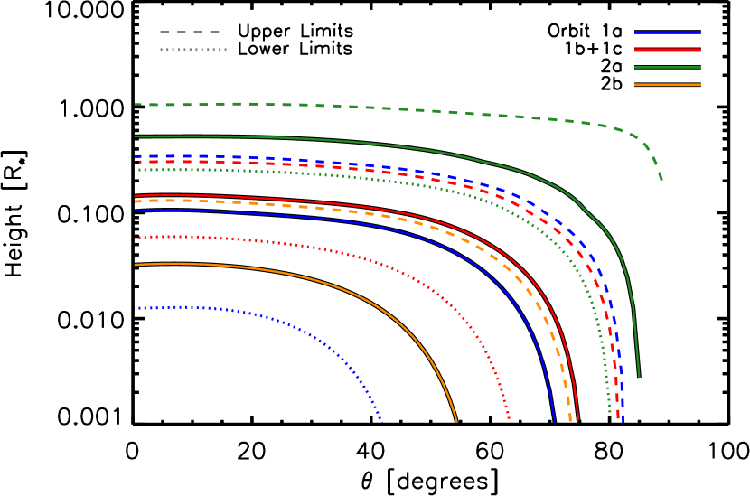
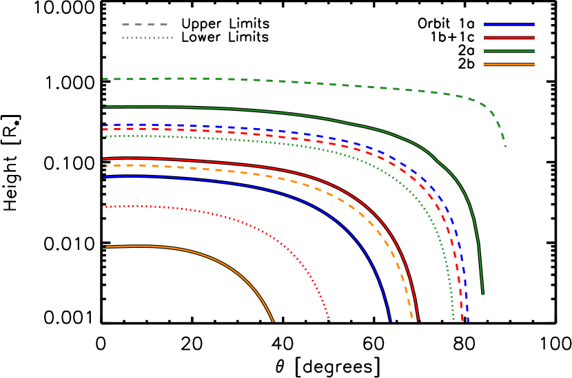
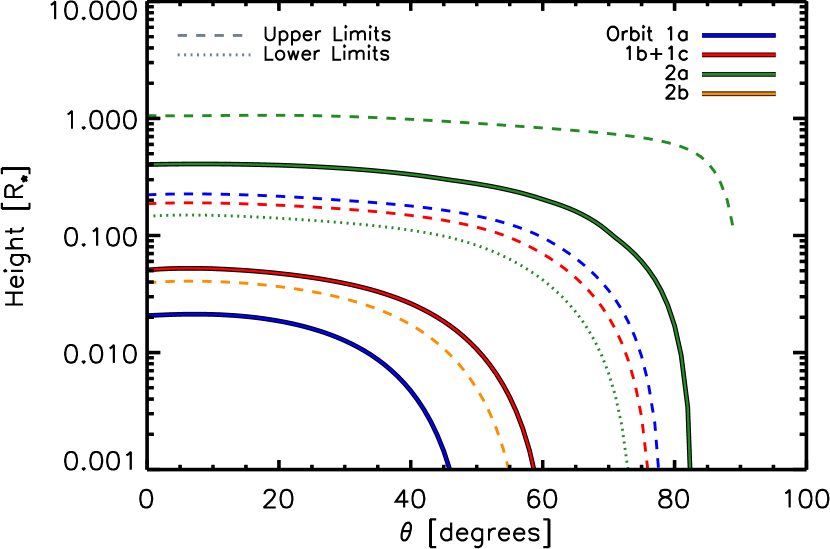
Figure 2.— Inferred flare height vs astrocentric angle for the different flare segments computed for the different photospheric metallicities considered here: [M/H]=0.0 (top); [M/H]$=-0.2$ (middle); and [M/H]$=-0.4$ (bottom). The observed X-ray spectral properties and Fe K$\alpha$ equivalent widths for segments 1b and 1c are essentially identical and have been averaged. The different segments are colour-coded, with upper and lower limits given by dashed and dotted curves, respectively.

The allowed ranges of flaring loop scale height derived from the strength of the Fe K line in the previous section can be compared with predictions from detailed hydrodynamic flare models. Here, we use the scaling laws for loop length, cross-sectional area and plasma density derived from hydrodynamic simulations by Reale (2007) in application to the light curve and plasma emission measure and temperature found from the Swift observations by O07.

Relevant quantities required by the Reale (2007) relations are the flare rise time $t_{M,3}$ (in units of $10^{3}$s), the maximum plasma temperature $T_{0,7}$ (in units of $10^{7}$ K), the peak emission measure $\Phi$ (cm^-3), and the $1/e$ decay time $\tau^{\prime}_{s}$ (s). We estimate the flare rise and decay times from Fig. 1 in O07 al. (2007), and take the flare temperature and emission measure data from their Table 2. Since we are interested in the peak flare temperature, we adopt the highest temperature obtained from their 3-temperature best-fit models. The final set of adopted parameters is

$$t_{M,3} \approx 2$$ (1)

$$T_{0,7} \approx 30$$ (2)

$$\Phi \approx 10^{56}$$ (3)

$$\tau^{\prime}_{s} \approx 9000$$ (4)

Here, we have assumed that the maximum plasma temperature is the value observed at the time of maximum density, and that this time corresponds to the peak in the observed flare emission. Since the flaring loop is a closed volume, the latter assumption is straightforward. However, as noted by Reale (2007), the maximum flare temperature can be reached some time after the peak density is reached; we allow for this in the analysis below.

4.1. Loop length

The flaring loop half-length can be estimated from the from rise time and the maximum plasma temperature, as given in Eqn. (12) of Reale (2007):

$$L_{9}\approx 3~{}\psi^{2}T_{0,7}^{1/2}t_{M,3}$$ (5)

where $L_{9}$ is the loop half-length in units of $10^{9}$ cm. The parameter $\psi$ is the ratio of the maximum plasma temperature to that at density maximum,

$$\psi=\frac{T_{0}}{T_{M}}.$$

From Fig. 2 of O07, it can be seen that the rise phase flattens toward the emission maximum; this suggests the flaring loop is close to equilibrium at the maximum and that, therefore, $\psi\approx 1$ and the assumption of maximum plasma temperature at the time of maximum density holds. To allow for deviations from this assumption, we also quote results for $\psi\approx 1.3$ (see examples given in Reale 2007). For $T_{0,7}\approx 30$, $t_{M,3}\approx 2$, $\psi\approx 1$

$$L_{9}\approx 30$$

For $\psi\approx 1.3$

$$L_{9}\approx 70$$

As a reasonable average value, we adopt $L_{9}\approx 50\pm 20$. Adopting a radius for II Peg of $3.4R_{\odot}$ (Berdyugina et al. 1998), this loop half-length corresponds to a loop height of $\sim 0.13R_{\star}$. This compares very favourably with the values we have estimated from the Fe K fluorescence line in the previous section, provided the flare were located toward the centre of the visible stellar disk and not toward the limb.

As a verification that this loop length value is reasonable, we can also obtain an estimate of the upper limit to $L_{9}$ from the decay timescale. If the decay is entirely driven by cooling, with no further heat input, the observed decay timescale can be equated with the thermodynamic decay time,

$$\tau^{\prime}_{s}=\phi\tau_{s}$$ (6)

where $\phi\approx 1.3$ and

$$\tau_{s}=3.7\times 10^{-4}\frac{L}{\sqrt{T_{0}}}=120\frac{L_{9}}{\sqrt{T_{0,7}}}$$ (7)

For $\tau^{\prime}_{s}\approx 9000$ s, we obtain an upper limit for the loop length:

$$L_{9}\leq 320.$$

While much larger, this upper limit is consistent with the value obtained from the rise phase above.

Huenemoerder et al. (2001) observed a large flare on II Peg during a 45 ks observation with the Chandra High Energy Transmission Grating Spectrometer (HETGS), during which the count rate was observed to rise to 2.5 times its quiescent value and the peak flare temperature reached $\log T\sim 7.6$. While much less intense than the Swift flare discussed here, the decay timescale of $\sim 65$ ks was somewhat longer. Huendmoerder et al. (2001) interpreted the light curve in terms of both single loop and two-ribbon type flares and inferred a loop height in the range 0.05–0.25 R_⋆ for the former, depending on the plasma density assumed. This height then scales inversely with the cube of the number of loops involved—e.g. smaller by a factor of  5 for 100 loop strands. While this estimate must be considered very approximate, the similarity with the loop height derived here for the Swift flare suggests that both events occurred in similar coronal structures that might be typical of the outer atmosphere of II Peg.

4.2. Plasma Density, Volume and Loop Cross-sectional Area

From Reale (2007), the maximum possible density equilibrium value at the loop apex in units of $10^{10}$ cm^-3 is given by

$$n_{0,10}=13\frac{T_{0,7}^{2}}{L_{9}}$$

While this is an upper limit, the true value should not be lower by more than a factor of 2. For $T_{0,7}\approx 30$ and $L_{9}\approx 50$, the density is then

$$n_{0,10}\leq 360$$

A reasonable value to adopt is $n_{0,10}\approx 200$. This value is compatible with density diagnostics from line ratios of hot He-like triplets, such as Mg xi, observed during flaring and quiescence on II Peg (Huenemoerder et al. 2001; Testa, Drake & Peres 2004). Similarly high densities have also been reported by Güdel et al. (2002) during an X-ray flare in Proxima Centauri. From Reale (2007), the volume is:

$$V\approx\frac{\Phi}{n_{avg}^{2}}$$ (8)

where

$$n_{avg}=n_{M}\frac{T_{M}}{T_{avg}}$$ (9)

Taking $T_{avg}\approx 150$ MK from the single temperature model fit of O07 (their Table 2), we obtain

$$n_{avg}\approx 4\times 10^{12}~{}~{}~{}~{}~{}\rm cm^{-3}$$

and

$$V\approx 6\times 10^{30}~{}~{}~{}~{}~{}\rm cm^{3}$$

The cross-sectional area is:

$$A\approx\frac{V}{2~{}L}$$ (10)

For $L_{9}\approx 50$, $A\approx 6\times 10^{19}$ cm². For a single loop with circular cross-section we obtain a radius in units of $10^{9}$ cm of $r_{9}\approx 4$, which is slightly less than 1/10 the loop half-length and very similar to the values found for solar flaring loops (e.g. Cheng et al. 1980, Golub et al. 1980, Peres et al. 1987).

4.3. Conductive energy losses

One of the most striking aspects of the Swift II Peg flare is the potentially large flare energy budget. Using the classical Spitzer formulism, O07 found an upper limit to the conductive losses of $5\times 10^{43}$ erg, but were unable to constrain this further without estimates of the flare dimensions and density. The bolometric luminosity of II Peg is $\log L_{bol}=34.2$ (Marino et al. 1999), and conductive losses as high as $10^{43}$ erg during a single, compact flare would represent an astounding concentration of energy.

We can refine the estimate of the conductive energy losses using Eqn. (5) in O07 and the parameters derived above for the flaring loop:

$$E_{cond}=\frac{\kappa T^{7/2}\Phi\Delta t}{L^{2}n_{e}^{2}},$$

where, for Orbit 1, $T\approx 300$ MK (an upper limit for the flare as a whole), $\Phi\approx 10^{56}$, $\kappa\approx 10^{-6}$ (in c.g.s. units), $\Delta t\approx 2$ ks, $L_{9}\approx 50$, $n_{e}\approx n_{avg}\approx 4\times 10^{12}$ cm^-3, we obtain

$$E_{cond}\leq 2\times 10^{36}~{}~{}~{}\rm erg$$

which is similar to the total radiated energy of $6\times 10^{36}$ erg in the 0.01-200 keV energy band estimated by O07. The duration of the flare was of order $10^{4}$s, and the radiative and conductive losses therefore represent an energy output of $\sim 10^{33}$ erg s^-1, or about 1/10 the stellar bolometric luminosity.

5. Conclusions

We have presented a set of Monte Carlo calculations able to reproduce the Fe K$\alpha$ equivalent widths from the Swift X-ray Telescope observations of II Peg during a ’superflare’ (Osten et al., 2007, O07). Our models show that the data are consistent with the Fe K$\alpha$ emission being produced by fluorescence following K-shell photoionisation of quasi-neutral iron in the stellar photosphere. This contrasts with the interpretation of O07, who favoured collisional ionisation by non-thermal electrons to produce the Fe K$\alpha$ emission. They argued that the normal incidence flare X-ray penetration depth required in the photosphere to obtain the observed equivalent widths is similar to the $\tau=1$ Compton scattering depth, and consequently any fluorescent photons produced would not easily escape. However, this assessment was based on a simple analytical formula appropriate for optically thin cases in which only a small fraction of the incident X-ray flux undergoes photoabsorption or scattering (e.g. Liedahl, 1999; Krolik & Kallman, 1987). The semi-infinite photospheric case lies outside the range of applicability of this formula. Furthermore, incident angles on the photosphere range from $\sim 0$–$90^{\circ}$ and path lengths for escape can therefore be much smaller than gas penetration depths (by a factor equal to the inverse cosine of these angles). Our stochastic treatment includes Compton scattering and shows that the observed equivalent widths can be produced by fluorescence. We also note that the impact excitation mechanism is a very low efficiency process and requires a large amount of energy in the form of accelerated electrons. This was already noted by, e.g., Parmar (1984) in reference to solar Fe fluorescence and by Ballantyne (2003), and was discussed in reference to a large flare on II Peg by Testa et al. (2008).

The derived flare loop heights are $h$ = 0.15 R_∗, assuming solar photospheric abundances, $h$ = 0.1 R_∗ assuming photospheric abundances depleted by [M/H] = -0.2 and $h$ = 0.06 R_∗ assuming [M/H] = -0.4. These value are in good agreement with the predictions from our alternative analysis based on hydrodynamic models (e.g. Reale, 2007) which yield $h\approx 0.13$ R_∗. We estimate flaring loop properties and energetics using scaling laws based on the hydrodynamic loop modeling of Reale (2007) and obtain a plasma density of $4\times 10^{12}$ cm^-3 and volume of $6\times 10^{30}$ cm³. Using the derived values for the flare dimensions and densities we obtain a more stringent upper limit for the conductive energy loss, $E_{cond}$, than previously possible, setting $E_{cond}\leq 2\times 10^{36}$ erg. Considering the duration of the flare and the radiative and conductive losses, the energy output of the flare is estimated at $\sim$10³³ erg sec^-1, which is approximately one tenth of the stellar bolometric luminosity.

While we cannot rule out a contribution to the observed Fe K$\alpha$ flux from electron impact with nonthermal electrons, as proposed by O07, such contribution is not necessary to explain the available data.

References

-
Ayres, T. R., Plymate, C., & Keller, C. U. 2006, ApJS, 165, 618
-
Basu, S., & Antia, H. M. 2008, Phys. Rep., 457, 217
-
Socas-Navarro, H., & Norton, A. A. 2007, ApJ, 660, L153
-
Berdyugina, S. V., Jankov, S., Ilyin, I., Tuominen, I., & Fekel, F. C. 1998, A&A, 334, 863
-
Cheng, C.-C., Tandberg-Hanssen, E., & Smith, J. B., Jr. 1980, Sol.Phys., 67, 259
-
Dere, K. P., Landi, E., Mason, H. E., Monsignori Fossi, B. C., & Young, P. R. 1997, A&AS, 125, 149
- Drake et al. (2008) Drake, J. J., Ercolano, B., & Swartz, D. A. 2008, ApJ, 678, 385, DES08
- Drake & Ercolano (2007) Drake, J. J., & Ercolano, B. 2007, ApJ, 665, L175
- Drake & Smith (1991) Drake, J. J., & Smith, G. 1991, MNRAS, 250, 89
- Drake et al. (2008) Drake, J. J., Ercolano, B., & Swartz, D. A. 2008, ApJ, 678, 385, DES08
-
Ercolano, B., Barlow, M. J., Storey, P. J., & Liu, X.-W. 2003a, MNRAS, 340, 1136
-
Ercolano, B., Young, P. R., Drake, J. J., & Raymond, J. C. 2007, ArXiv e-prints, 710, arXiv:0710.2103
-
Golub, L., Maxson, C., Rosner, R., Vaiana, G. S., & Serio, S. 1980, ApJ, 238, 343
-
Güdel, M., Audard, M., Skinner, S. L., & Horvath, M. I. 2002, ApJ, 580, L73
-
Huenemoerder, D. P., Canizares, C. R., & Schulz, N. S. 2001, ApJ, 559, 1135
-
Krolik, J. H., & Kallman, T. R. 1987, ApJ, 320, L5
-
Landi, E., Del Zanna, G., Young, P. R., Dere, K. P., Mason, H. E., & Landini, M. 2006, ApJS, 162, 261
-
Liedahl, D. A. 1999, X-Ray Spectroscopy in Astrophysics, 520, 189
-
Marino, G., Rodonó, M., Leto, G., & Cutispoto, G. 1999, A&A, 352, 189
-
Osten, R. A., Drake, S., Tueller, J., Cummings, J., Perri, M., Moretti, A., & Covino, S. 2007, ApJ, 654, 1052
-
Peres, G., Reale, F., Serio, S., & Pallavicini, R. 1987, ApJ, 312, 895
-
Reale, F. 2007, A&A, 471, 271
- Testa et al. (2004) Testa, P., Drake, J. J., & Peres, G. 2004, ApJ, 617, 508
-
Testa, P., Drake, J. J., Ercolano, B., Reale, F., Huenemoerder, D. P., Affer, L., Micela, G., & Garcia-Alvarez, D. 2008, ApJ, 675, L97