Testing a priority-based queue model with Linux command histories

Abstract

We study human dynamics by analyzing Linux history files. The goodness-of-fit test shows that most of the collected datasets belong to the universality class suggested in the literature by a variable-length queueing process based on priority. In order to check the validity of this model, we design two tests based on mutual information between time intervals and a mathematical relationship known as the arcsine law. Since the previously suggested queueing process fails to pass these tests, the result suggests that the modelling of human dynamics should properly consider the statistical dependency in the temporal dimension.

, ,

1 Introduction

Recently, there have been various attempts to characterize the human behaviors in mathematical terms which have been successfully applied to natural phenomena. To name a few, the human activities like Internet, traffic flows, family names and stock prices are under active investigation and give deep insights into our society [1, 2, 3, 4, 5, 6]. Now we have even a popularized term known as ‘human dynamics’ [7], and many researchers are devoting themselves to this field. One of their most surprising claims is that there exist a few universality classes in human dynamics [8, 9, 10]. Those universality classes are described by a priority-based queuing process, which yields power-law waiting-time distributions $p(\tau)\sim\tau^{-\alpha}$ with universal exponents of $\alpha=1.0,1.5$, and $2.5$ [11]. This idea has generated great public attention due to its philosophical implications against our conventional belief in human conditions, and there have been also intensive scientific debates on their observations [12] and on the existence of universality classes [13]. Even if one may doubt the validity of the universality claim, their original observation truly pointed out some fundamental properties of human behaviors and contributed a lot to this field by proposing a powerful and falsifiable model. To our knowledge, only a few models are yet to undergo closer examinations, including those in Refs. [14, 15].

In this article, we analyze human behaviors through Linux history files, which contain the histories of every shell command input by terminals. Unlike the records in supercomputers [16] and personal computers including mouse movements [17], our observation partially supports the universality claim in that most of the collected distributions fall into the suggested universality class with $\alpha=1.5$. Since this is the regime where a priority-based queue model works with varying the queue length [8], we may imagine that a person works as the model describes, where each command executed on the shell introduces the next command to her queue with a randomly assigned priority. The waiting time before execution is essentially dominated by a random walk of the queue length, which gives the desired power-law distribution with $\alpha=1.5$ [18]. However, the overall distribution shows only a small amount of information and it is more than possible to devise further examinations to compare our empirical data with the suggested model. In other words, if command inputs can be described by the queue model which reduces to a one-dimensional random walker, such a simple and rigorous mechanism should put some explicitly testable constraints on the result. For example, a natural requirement is that the time intervals between two consecutive events must be mutually independent of each other. That is our motivation to design two tests based on the correlation between time intervals and the characteristic hitting time distribution as a regenerative process [19], respectively. These tests prove that our observations are not fully explained by the existing queue models.

This article is organized as follows: In Sec. 2, we explain how we prepared datasets and present their basic statistical features. In Sec. 3, the goodness-of-fit test for verifying power-law behaviors is followed by two tests to examine the priority-based queue model. Then we discuss the implications of the test results in Sec. 4 and conclude this work in Sec. 5.

2 Data Collection

A Linux system usually keeps every user’s shell command history up to some predefined length. In Bash (Bourne-again shell), each shell command can be made accompanied by a time-stamp, if we add a couple of lines to a resource file called ‘.bashrc’ as in Fig. 1(a), where the first line defines the maximal history length and the second adds time-stamps. Then a user’s typical history is written as in Fig. 1(b) with the numbers indicating time-stamps in units of second. We collect seven history files from six users (including two authors of the present paper), each of which is given an alphabet from $A$ to $G$. Since they worked without any explicit coordination during the recording period, we regard these records as mainly reflecting their individual characteristics. Note that the history files may not be arranged in a chronological order when a user uses multiple terminals so that we have to sort the datasets before analyses. In addition, we generate one more dataset $R$, recording the return times of a one-dimensional random walker to the origin, which will function as a control group throughout our analyses. Fig. 2 shows the input rates for the datasets $A$ and $R$ by counting the number of events in every hour, or in $60^{2}=3600$ time units (seconds).

Letting $t_{i}$ indicate the time when the $i$th command was entered, we define the waiting time $\tau_{i}$ between two consecutive inputs as

$$\tau_{i}\equiv t_{i+1}-t_{i}.$$

Conversely, if there are $n$ command inputs recorded in the file, $T\equiv\sum_{i=1}^{n}\tau_{i}$ is the total time interval. There are two other characteristic quantities, $\bar{\tau}\equiv T/n$ and $\tau_{\rm max}\equiv\max_{i}\{\tau_{i}\}$, although we will see later that $\bar{\tau}$ is not a good statistic in that it is essentially sample-dependent here. Those values for each dataset are listed in Table 1.

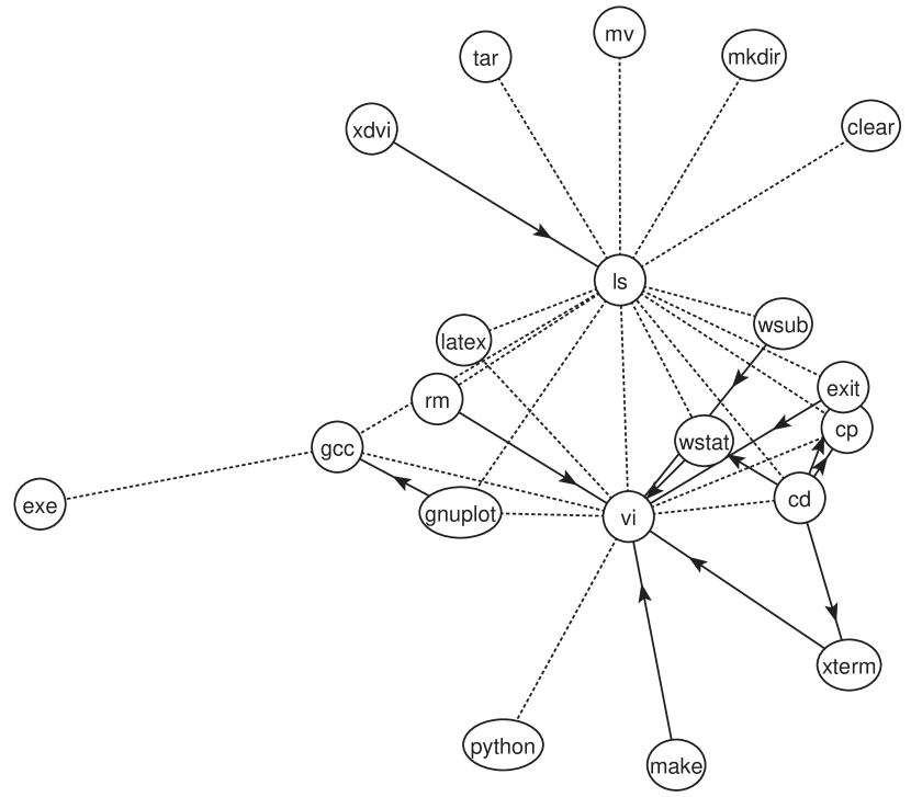
Figure 3: Command input pattern of the dataset $A$. Self-loops are omitted, and the dahsed edges without arrows represent the transitions in both directions. The commands named as ‘wsub’ and ‘wstat’ are not supported by ordinary Linux shells but specific to this Linux machine, while ‘exe’ indicates all the user-generated executable files.

Furthermore, one may be interested in the transition between commands. Suppose that when a command $c_{1}$ is followed by a command $c_{2}$ in the shell, we call it a transition from $c_{1}$ to $c_{2}$. The transition patterns are easily visualized by a network, as shown in Fig. 3 by nodes (commands) and links (transitions). As the largest frequency is found in the transition from ‘ls’ to ‘cd’, only those links are depicted whose transition frequencies exceed $2\%$ of it, together with the major commands involved in these transitions.

3 Data Analysis

3.1 Waiting-time distribution

Let us consider the probability distribution $p(\tau)$, obtained from an empirical dataset, $\{\tau_{i}\}$. For convenience, we are going to work with its derived form, the cumulative distribution function defined as follows [18]:

$$P(\tau)=\int_{\tau}^{\infty}p(\tau^{\prime})~{}d\tau^{\prime}.$$

Fig. 4 displays $P(\tau)$’s for our eight datasets. The distribution function in Fig. 4(d) looks far from a straight line, presumably because this user prefers using his own personal Linux machine to accessing the remote server where the recording has been carried out. In comparison, the distribution in Fig. 4(e) which is for the same user as in (d) (he submitted two history files $D$ from a remote server and $E$ from his own local desktop, respectively) does not show any significant difference from other datasets. It evidently shows an effect of individual characteristics, and the concave shape is reminiscent of the job submission interval in supercomputers [16]. Nevertheless, if we exclude the dataset $D$, the qualitative behaviors are surprisingly similar to each other.

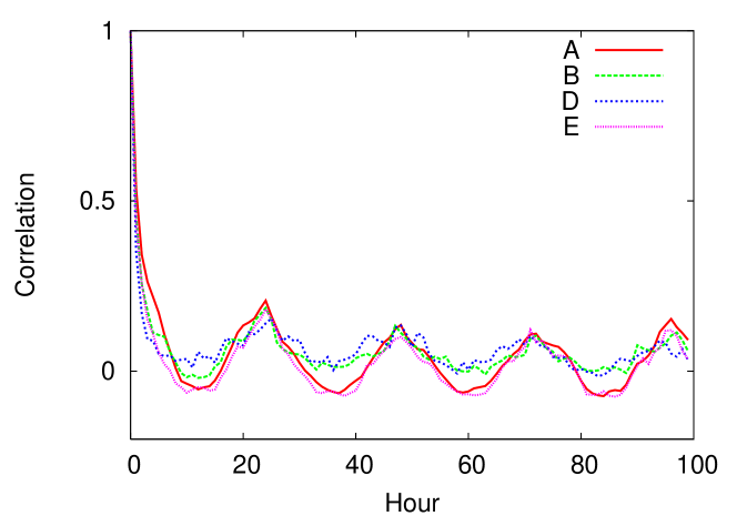
Figure 6: (Color online) Autocorrelation of input rates in each dataset. We depict only four datasets which clearly show oscillatory patterns with a period of $24$ h.

Every arrow in Fig. 4 indicates the point at $4.32\times 10^{4}$ s, or $12$ h. The existence of a hump for each individual appears to reflect his daily life cycle. The Fourier transform also confirms that the working pattern is quite regular, as two peaks are prominent at one day and one week (Fig. 5). Shown differently, the autocorrelation function from the input rate [2] exhibits oscillatory patterns with periods around $24$ h (Fig. 6). All of these indicate the existence of long-term orders.

We fit each dataset using a power-law function $p(\tau)\sim\tau^{-\alpha}$ with an appropriate lower bound $\tau_{\rm min}$, where the number of data points larger than or equal to $\tau_{\rm min}$ is denoted as $n_{\rm tail}$. The optimal parameter values are listed in Table 2. We apply the goodness-of-fit test based on the Kolmogorov-Smirnov (KS) statistic and measure the $p$-value, the probability that a dataset was drawn from the hypothesized distribution [20]. As shown by $p$-values in Table 2, the power-law function is found to be at least a moderate description for all the datasets except $D$. The humps due to long-term orders do little harms in the test, because the KS test tends to be sensitive to the deviations in the body part, rather than those in the tail part with a much smaller scale. We do not treat the model selection problem [20] here, but it would not be a big surprise if they converge to the Lévy stable distribution in the long run by the generalized Central Limit Theorem.

3.2 Mutual information

To further analyze behavioral patterns, some authors employ the conventional autocorrelation function [21]:

$$a(j)=\frac{1}{n-j}\sum_{i=1}^{n-j}(\tau_{i}-\bar{\tau})(\tau_{i+j}-\bar{\tau}).$$

Note that this function assumes the well-behavedness of statistical moments such as the average $\bar{\tau}$. None of them are well defined for power-law distributions with $\alpha\leq 2$ [18], and the large variation of $\bar{\tau}$ in Table 1 implies this deficiency.

We next try to devise an alternative measure for the correlation, which should be zero for perfectly uncorrelated data. A possible trick is reverting the generation algorithm for power-law distributed random numbers: If $r$ is a random number uniformly drawn from $[0,1)$, the formula given as

$$x=x_{\rm min}(1-r)^{-1/(\alpha-1)}$$

makes a power-law distribution $p(x)\sim x^{-\alpha}$ with a lower bound $x_{\rm min}$ [20]. Therefore, if $\{x_{i}\}$ is a set of power-law distributed random numbers, the inverse transformation

$$r_{i}=1-\left(\frac{x_{i}}{x_{\rm min}}\right)^{1-\alpha}$$

will generate a set of random numbers uniformly distributed between $[0,1)$. In discrete case as ours, each $x_{i}$ is not mapped to a unique point, but to a set of points ranged over

$$\left[1-\left(\frac{x_{i}-\frac{1}{2}}{x_{\rm min}-\frac{1}{2}}\right)^{1-\alpha},1-\left(\frac{x_{i}+\frac{1}{2}}{x_{\rm min}-\frac{1}{2}}\right)^{1-\alpha}\right).$$

Since every number within this range is equivalent, a reasonable choice is to draw a point $r_{i}$ randomly within the interval. This indeterminacy makes some fluctuations on the final result, but this trick still works giving us consistent estimates. The mutual information between consecutive points is then calculated as [22]

$$I(r_{i+1};r_{i})=\sum_{r_{i}}\sum_{r_{i+1}}p(r_{i+1},r_{i})\log\left[\frac{p(r_{i+1},r_{i})}{p(r_{i+1})p(r_{i})}\right],$$ (1)

where $p(r_{i+1},r_{i})$ means the joint probability density function of $r_{i+1}$ and $r_{i}$. Accordingly, if $r_{i}$ and $r_{i+1}$ are completely uncorrelated, $I$ takes the null value.

Applying this transformation to each collected dataset, $\{\tau_{i}\}$, we obtain the transformed result, $\{u_{i}\}$, whose number of elements is $n_{\rm tail}$. Introducing $H_{1}=-\sum p(u_{i})\log p(u_{i})$ and $H_{2}=-\sum p(u_{i+1},u_{i})\log p(u_{i+1},u_{i})$ as the entropy of $\{u_{i}\}$ and the joint entropy of $\{u_{i+1},u_{i}\}$, respectively, we rewrite Eq. (1) as follows:

$$I(u_{i+1};u_{i})=2H_{1}-H_{2}.$$

Normalizing this with respect to the entropy, we get the following quantity to measure how much correlation a dataset contains:

$$h=1-\frac{H_{2}}{2H_{1}}.$$

In practice, $p(u)~{}du$ is estimated by the number of data points between $[u,u+du)$, and the values of entropies are dependent on the choice of $du$, or equivalently, the number of bins in making a histogram. We choose Sturges’ formula to determine the optimal number of bins [23]:

$$k=\lceil\log_{2}n_{\rm tail}+1\rceil,$$

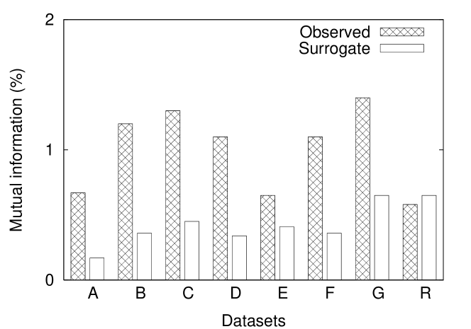
Figure 7: Mutual information between consecutive time intervals for the observed datasets and their surrogates.

where $\lceil x\rceil$ means the ceiling function of $x$. The results are shown in Fig. 7. Every $h$ lies at around $1\%$, which is not much larger than our expectation. However, we have to check if those values are small enough to conclude that the data are indeed uncorrelated. A common technique to find a reference point is by using surrogates [22]: To destroy all the possible correlation without altering the overall distribution, it suffices to perform a random shuffle on the data. Then we calculate the mutual information from an ensemble of such surrogate datasets. As shown in Fig. 7, while this method makes little differences in $R$, every other human dataset is found to carry mutual information to a significant degree. Therefore this implies that our datasets have differences from what the previously proposed priority-based queue model predicts from the viewpoint of mutual information.

Before proceeding, however, some subtlety should be mentioned: Since this test simply neglects all the $\tau_{i}$’s smaller than $\tau_{\rm min}$, some pairs of $(u_{i},u_{i+1})$ may not come from the really consecutive time intervals. If we further require such consecutiveness, the number of available data pairs becomes even less than $n_{\rm tail}$, making the results also unclear for some datasets. Therefore, even though we could reveal some quantitative differences, they are not so conclusive as the constraint $\tau>\tau_{\rm min}$ and the indeterminacy for a discrete case severely worsen the power of this test. It is for the reason that we newly propose another test, taking all the data points into consideration.

3.3 Arcsine test

Suppose that a one-dimensional random walker in the $x$-direction starts at time $t=0$ from the origin at $x=0$. It is then mathematically proved that the probability $f$ for the walker to hit the origin ($x=0$) in the time interval $(\xi t,t)$ with $0<\xi<1$ is given by [19]

$$f(\xi)=1-\frac{2}{\pi}{\rm arc}\sin\sqrt{\xi},$$ (2)

as $t\rightarrow\infty$. Let us check how much our datasets are away from this result. For a given $t$, we can estimate the probability function, $\eta=f_{e}(\xi)$, from our datasets with varying $\xi$. It is a monotonically decreasing function by definition, and the following KS statistic will properly quantify the the maximum deviation [24]:

$$d=\max_{\eta}|f_{e}^{-1}(\eta)-f^{-1}(\eta)|.$$ (3)

Note that since each measured point should contribute an equal amount in the KS test, the inverse functions are more appropriate. Due to the assumption that $t\rightarrow\infty$ which Eq. (2) is based on, we observe how the statistic $d$ behaves as $t$ increases (Fig. 8). We only use the time $t$ less than $10\%$ of the total recording period $T$ in order to avoid effects caused by the finiteness of the time. As clearly shown in Fig. 8, only the dataset $R$ maintains low $d$ at large $t$. Moreover, one may easily calculate the significance level from the fact that $f_{e}(\xi)$ is constructed with the effective number of points $N_{e}=49$ (see Ref. [24] for details of the KS test): The dataset $R$ has $d\approx 0.12$ at $t\approx 0.1T$ which amounts to the significance level of $Q_{KS}\approx 46\%$. Even if this does not satisfy the usual requirement like $95\%$ significance level, it is still remarkable since we observe that every other human dataset has $Q_{KS}<10^{-20}$ under the same condition. Consequently, it is very plausible that the human dynamics in our datasets needs a modified description than a simple random walker, which is also supported by the previous test based on the mutual information.

4 Discussion

One interesting point in our observation is that the datasets show heavy-tailed distributions up to some cutoffs and, at the same time, quite regular behaviors. This is seemingly contradictory, as a power-law distribution with an exponent $\alpha\leq 2$ is known to make its average and variance diverge, lacking any characteristic time scales.

Even though one may say that the irregularity still exists in intra-day scales at least (see Fig. 4), it is true that a power-law distribution does not necessarily imply highly complicated dynamics. Let us consider a very simple example with $N$ persons, each of whom has her own working frequency, $f_{i}~{}~{}(i=1,\cdots,N)$. If these frequencies are uniformly distributed for a rather wide range of time scales, the collected set of waiting times will have a power-law distribution. Namely, the number of each person’s own time interval is simply an inverse quantity of $f_{i}$, and should have the following distribution [18]:

$$p(\tau)=p(f)\left|\frac{df}{d\tau}\right|=\frac{p(f)}{\tau^{2}}\sim\tau^{-2}.$$

Even a single person may have multiple working phases, each of which requires a different frequency of inputs but occupies roughly the same time as other phases. Indeed, the exponent $\alpha\approx 2$ is already reported in Refs. [13, 17], and modulating the exponent is not impossible because any random parts in fragmenting time schedules are basically a multiplicative process yielding power-law or log-normal distributions [25].

This is an illustrative, if not serious, example to show that there may be a number of competing theories, all of which yield power-law distributions with being totally different in other respects [18]. We have thus focused on consistency checks for a previously suggested model, while leaving how to elaborate on a new one to be a future work. We stress that rejecting the existing queue model in our case does not mean that it is wrong or useless. Rather, our study shows one of its greatest virtues, i.e., the openness to a variety of challenges. Therefore, the queueing scheme is still a good starting point to consider human behaviors at the first approximation in a variety of situations, once one keeps in mind how a current simple model may deviate from reality.

5 Conclusion

We collected human behavioral patterns from Linux history files and found that their waiting-time distributions followed power-laws. Since they seemed to fall into the previously claimed universality class, characterized by an exponent of $1.5$, we tested the corresponding priority-based queue model by two measures. The first test was based on the mutual information, while the second was on the arcsine law in a regenerative process. Both tests indicated that our datasets had significant differences from what the model of our concern predicted. This implies that we should also consider the temporal relations in order to find an accurate description of human behaviors.

Figure 1: (a) Two lines added to .bashrc to record time-stamps up to $10^{6}$ lines. (b) A typical look at the resulting history file, which contains one time-stamp above every command input to the Linux shell.

Figure 2: (a) Command input rate of the dataset $A$, measured by the number of inputs in every hour ($=3.6\times 10^{3}$ s). (b) A one-dimensional random walker’s number of return to the origin in every hour ($=3.6\times 10^{3}$ time steps), from the dataset $R$.

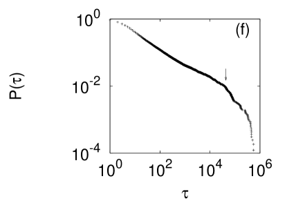
Figure 4: Cumulative distributions of waiting times in collected datasets. The panels from (a) to (g) correspond to the empirical datasets from $A$ to $G$, respectively, while the panel (h) indicates the dataset $R$ from a random walker. Each arrow indicates $\tau=12$ h.

Figure 5: Fourier transformation of input rates in the dataset $A$.

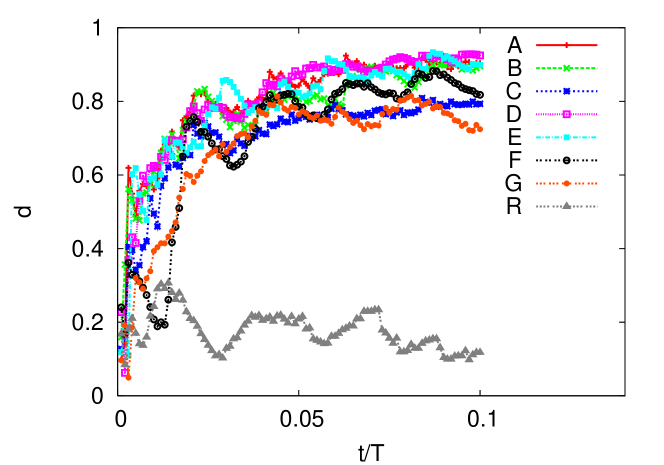
Figure 8: (Color online) Deviation $d$ between the estimated probability function and the arcsine law [see Eq. (3) and text] as $t$ increases up to $10\%$ of the total recording period, $T$. Except for $R$ from the random walk, all datasets are shown not to converge to the arcsine law.

Table 1: Basic quantities: Datasets were collected from seven history files (A–G) and R was generated by a simple computer program simulating a one-dimensional random walk. The columns titled as $n$ and $T$ are the number of recorded commands and the total recording period, respectively. The third column gives the average time interval $\bar{\tau}\equiv T/n$, while the last one shows the maximal interval in each dataset.

Dataset	$n$	$T$	$\bar{\tau}$	$\tau_{\rm max}$
A	$9.3\times 10^{4}$	$2.9\times 10^{7}$	$3.1\times 10^{2}$	$1.1\times 10^{6}$
B	$2.2\times 10^{4}$	$2.9\times 10^{7}$	$1.3\times 10^{3}$	$1.0\times 10^{6}$
C	$1.3\times 10^{4}$	$2.9\times 10^{7}$	$2.1\times 10^{3}$	$2.4\times 10^{6}$
D	$3.0\times 10^{4}$	$2.7\times 10^{7}$	$8.9\times 10^{2}$	$1.4\times 10^{6}$
E	$4.8\times 10^{4}$	$2.1\times 10^{7}$	$4.4\times 10^{2}$	$5.2\times 10^{5}$
F	$1.6\times 10^{4}$	$2.9\times 10^{7}$	$1.8\times 10^{3}$	$1.8\times 10^{6}$
G	$1.2\times 10^{4}$	$1.5\times 10^{7}$	$1.2\times 10^{3}$	$1.2\times 10^{6}$
R	$2.0\times 10^{4}$	$1.3\times 10^{8}$	$6.3\times 10^{3}$	$3.0\times 10^{7}$

Table 2: Results of the goodness-of-fit test: Each dataset is fitted to the power-law distribution with a lower bound $\tau_{\rm min}$ and an exponent $\alpha$ by the KS test. The number of points satisfying $\tau_{i}\geq\tau_{\rm min}$ is denoted as $n_{\rm tail}$, and a $p$-value means the probability that the power-law hypothesis is correct.

Dataset	$\tau_{\rm min}$	$\alpha$	$n_{\rm tail}$	$p$-value
A	60	1.74	$1.1\times 10^{4}$	0.47
B	24	1.47	$4.4\times 10^{3}$	0.34
C	32	1.50	$3.1\times 10^{3}$	0.61
D	13	1.57	$4.8\times 10^{3}$	0.00
E	174	1.62	$3.5\times 10^{3}$	0.62
F	25	1.48	$3.9\times 10^{3}$	0.22
G	26	1.52	$2.2\times 10^{3}$	0.20
R	36	1.50	$1.9\times 10^{3}$	0.84

References

- [1] R. Albert, H. Jeong, A.-L. Barabási, The diameter of the world wide web, Nature 401 (1999) 130.
- [2] B. Kujawski, J. Holyst, G. J. Rodgers, Growing trees in Internet news groups and forums, Phys. Rev. E 76 (2007) 036103.
- [3] W.-X. Wang, B.-H. Wang, C.-Y. Yin, Y.-B. Xie, T. Zhou, Traffic dynamics based on local routing protocol on a scale-free network, Phys. Rev. E 73 (2006) 026111.
- [4] B. J. Kim, S. M. Park, Distribution of Korean family names, Physica A 347 (2005) 683.
- [5] S. K. Baek, H. A. T. Kiet, B. J. Kim, Family name distributions: master equation approach, Phys. Rev. E 76 (2007) 046113.
- [6] H. A. T. Kiet, S. K. Baek, H. Jeong, B. J. Kim, Korean family name distribution in the past, J. Korean Phys. Soc. 51 (2007) 1812.
- [7] A.-L. Barabási, The origin of bursts and heavy tails in human dynamics, Nature 435 (2005) 207.
- [8] J. G. Oliveira, A.-L. Barabási, Darwin and Einstein correspondence patterns, Nature 437 (2005) 1251.
- [9] A. Vázquez, Exact results for the Barabási model of human dynamics, Phys. Rev. Lett. 95 (2005) 248701.
- [10] A. Vázquez, J. G. Oliveira, Z. Dezsö, K.-I. Goh, I. Kondor, A.-L. Barabási, Modeling bursts and heavy tails in human dynamics, Phys. Rev. E 73 (2006) 036127.
- [11] G. Grinstein, R. Linsker, Biased diffusion and universality in model queues, Phys. Rev. Lett. 97 (2006) 130201.
- [12] D. B. Stouffer, R. D. Malmgren, L. A. N. Amaral, Comment on the origin of bursts and heavy tails in human dynamics, e-print arXiv: physics/0510216v1 (2005); A.-L. Barabási, K.-I. Goh, A. Vázquez, Reply to comment on “the origin of bursts and heavy tails in human dynamics”, e-print arXiv: physics/0511186 (2005).
- [13] T. Zhou, H. Kiet, B. J. Kim, B.-H. Wang, Role of activity in human dynamics, e-print arXiv: 0711.4168 (2007).
- [14] A. Vázquez, Impact of memory on human dynamics, Physica A 373 (2006) 747.
- [15] P. Blanchard, M.-O. Hongler, Human activity modeling and Barabási’s queueing systems, e-print arXiv: cond-mat/0608156v1 (2006).
- [16] S. D. Kleban, S. H. Clearwater, Hierarchical dynamics, interarrival times, and performance, Proc. SC2003 (2003).
- [17] H. P. Slijper, J. M. Richter, J. B. J. Smeets, M. A. Frens, The effects of pause software on the temporal characteristics of computer use, Ergonomics 50 (2007) 178.
- [18] M. E. J. Newman, Power laws, Pareto distributions and Zipf’s law, Contemp. Phys. 46 (2005) 323.
- [19] S. M. Ross, Stochastic Processes, 2nd Edition, John Wiley & Sons, New York, 1996.
- [20] A. Clauset, C. R. Shalizi, M. E. J. Newman, Power-law distributions in empirical data, e-print arXiv:0706.1062 (2007).
- [21] U. Harder, M. Paczuski, Correlated dynamics in human printing behavior, Physica A 361 (2006) 329.
- [22] H. Kantz, T. Schreiber, Nonlinear Time Series Analysis, Cambridge University Press, Cambridge, 1997.
- [23] H. A. Sturges, The choice of a class interval, J. Am. Stat. Assoc. 21 (1926) 65.
- [24] W. H. Press, S. A. Teukolsky, W. T. Vetterling, B. P. Flannery, Numerical Recipes in C, 2nd Edition, Cambridge University Press, New York, 2002.
- [25] D. Sornette, R. Cont, Convergent multiplicative processes repelled from zero: Power laws and truncated power laws, J. Phys. I 7 (1997) 431.