The inequality of charge and spin diffusion coefficients

Abstract

Since spin and charge are both carried by electrons (or holes) in a solid, it is natural to assume that charge and spin diffusion coefficients will be the same. Drift-diffusion models of spin transport typically assume so. Here, we show analytically that the two diffusion coefficients can be vastly different in quantum wires. Although we do not consider quantum wells or bulk systems, it is likely that the two coefficients will be different in those systems as well. Thus, it is important to distinguish between them in transport models, particularly those applied to quantum wire based devices.

In the drift-diffusion model of spin transport, it is customary to assume that the same diffusion coefficient ‘$D$’ describes charge and spin diffusion. This assumption is commonplace in the literature (see, for example, refs. zhang ; mishchenko ; burkov ; saikin ; pershin ). Ref. malshukov considers a two dimensional system with different spin and charge diffusion coefficients but ultimately assumes that the bare spin diffusion coefficient is the same as the charge diffusion coefficient. Ref. flatte also examines this issue, and based on an heuristic assumption that spin transport is analogous to bipolar charge transport, reaches the conclusion that the two diffusion coefficients are equal as long as the populations of upspin and downspin carriers are equal. In spin polarized transport, the two populations are unequal by definition. Therefore, it is imperative to examine if these two diffusion coefficients are still equal in spin polarized transport, and if not, then how unequal they can be. In this paper, we show that these two diffusion coefficients can be vastly different in quantum wires. Although we do not consider quantum wells and bulk systems, there is no reason to believe apriori that even in those systems, the two diffusion coefficients will be equal.

We first consider a narrow semiconductor quantum wire where only the lowest subband is occupied by carriers at all times. All higher subbands are unoccupied. We will assume that there are Rashba rashba and Dresselhaus dresselhaus spin orbit interactions in the wire, but no external magnetic field to cause spin mixing cahay . In that case, we can ignore the Elliott-Yafet spin relaxation mechanism elliott since it will be very weak. Spin relaxation via hyperfine interaction with nuclear spins, or via the Bir-Aronov-Pikus mechanism bap , is also typically very weak in semiconductor quantum wires with only one kind of carriers (electrons or holes, but not both). Therefore, the only spin relaxation mechanism that is important is the D’yakonov-Perel’ relaxation dp .

In the single channeled quantum wire, we will prove two remarkable results: (i) spin will relax in time (i.e. the spin relaxation time $\tau_{s}$ will be finite), but it will not relax in space (i.e. the spin relaxation length $L_{s}$ will be infinite), and (ii) if the drift-diffusion model is valid in this system (this model relates $L_{s}$ and $\tau_{s}$ as $L_{s}$ = $\sqrt{D_{s}\tau_{s}}$), then we must conclude that the spin diffusion coefficient $D_{s}$ is infinite. However, since there is scattering in the system, the charge diffusion coefficient $D_{c}$ must be finite. Therefore, the two diffusion coefficients are completely different. This is an extreme case, but even in less extreme cases (multi-channeled quantum wires), these two coefficients can be very different. Below, we provide an analytical proof for the single channeled quantum wire case.

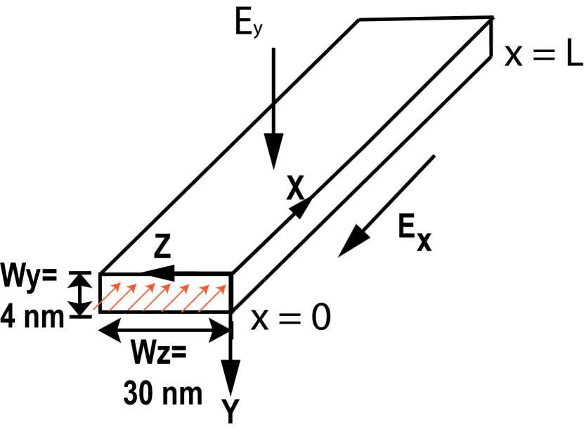
Figure 1: Pramanik et al.

Consider an ensemble of electrons injected in a quantum wire at time $t=0$ from the end $x=0$ as shown in Fig. 1. Only the lowest subband is occupied in the wire at all times. There is an electric field $E_{x}$ driving charge transport, and there is also a transverse electric field $E_{y}$ breaking structural inversion symmetry, thereby causing a Rashba spin orbit interaction rashba . We will assume that the quantum wire axis is along the [100] crystallographic direction and that there is crystallographic inversion asymmetry along this direction giving rise to Dresselhaus spin-orbit interaction dresselhaus . We choose this system because it is the simplest and includes the two major types of spin orbit interactions found in semiconductor nanostructures, namely the Rashba and the Dresselhaus interactions. Ref. pershin has considered this system within the framework of the drift-diffusion model and shown that there is a single time constant describing spin relaxation. In contrast, spin relaxation in a two-dimensional system (quantum well) may be described by more than one time constant pershin .

For illustration purposes, we will assume hypothetically that the spin injection efficiency is 100%, so that at $x=0$, all electrons are spin polarized along some particular, though arbitrary, direction $\hat{\eta}_{0}$ in space. Their injection velocities are not necessarily the same (in fact, they will be drawn from the Fermi-Dirac distribution in the contact). We are interested in finding out how the net spin polarization of the ensemble ($|\langle\bf S\rangle|$) decays in time or space due to the D’yakonov-Perel’ process.

In the quantum wire, the electrons experience various momentum relaxing scattering events. Between successive scattering events, they undergo free flight and during this time, their spins precess about a velocity-dependent pseudo-magnetic field ${\bf B_{so}}(v_{x})$ caused by Rashba and Dresselhaus spin-orbit interactions. This magnetic field can be shown to be spin-independent.

The spin precession of every single electron occurs according to the well-known Larmor equation:

$${{d{\bf S}}\over{dt}}={\bf\Omega}(v_{x})\times{\bf S},$$ (1)

where ${\bf S}$ is the spin polarization vector of the electron and ${\bf\Omega}(v_{x})$ is a vector whose magnitude is the angular frequency of spin precession. It is related to ${\bf B_{so}}(v_{x})$ as ${\bf\Omega}(v_{x})=(g\mu_{B}/\hbar){\bf B_{so}}(v_{x})$, where $g$ is the Landé g-factor in the material and $\mu_{B}$ is the Bohr magneton. This is actually the well-known equation for Larmor spin precession and can be derived rigorously from the Ehrenfest Theorem of quantum mechanics.

The vector ${\bf\Omega}(v_{x})$ has two contributions due to Dresselhaus and Rashba interactions:

$${\bf\Omega}(v_{x})={\bf\Omega_{D}}(v_{x})+{\bf\Omega_{R}}(v_{x}),$$ (2)

where the first term is the Dresselhaus and the second term is the Rashba contribution. These two contributions are given by

$${\bf\Omega_{D}}(v_{x}) = {{2m^{*}a_{42}}\over{\hbar^{2}}}\left[\left({{\pi}\over{W_{y}}}\right)^{2}-\left({{\pi}\over{W_{z}}}\right)^{2}\right]v_{x}\hat{x}=\zeta_{D0}v_{x}\hat{x}$$

$${\bf\Omega_{R}}(v_{x}) = {{2m^{*}a_{46}}\over{\hbar^{2}}}E_{y}v_{x}\hat{z}=\zeta_{R0}v_{x}\hat{z},$$ (3)

where $W_{z},W_{y}$ are the transverse dimensions of the wire, $a_{42}$ and $a_{46}$ are material constants, $\hat{x}$ is the unit vector along the x-direction and $\hat{z}$ is the unit vector along the z-direction.

Note that the vector ${\bf\Omega}$ lies in the x-z plane and subtends an angle $\theta$ with the $\pm$x-axis (quantum wire axis) given by

$$\theta=arctan\left[{{\zeta_{R0}}\over{\zeta_{D0}}}\right]=arctan\left[{{a_{46}E_{y}}\over{a_{42}\left\{\left({{\pi}\over{W_{y}}}\right)^{2}-\left({{\pi}\over{W_{z}}}\right)^{2}\right\}}}\right].$$ (4)

Note also that since $\theta$ is independent of $v_{x}$, the axis (but not the magnitude) of both ${\bf\Omega}$ and ${\bf B_{so}}$ is independent of electron velocity. Therefore, every electron, regardless of its velocity, precesses about the same axis, as long as only one subband is occupied. The direction of precession (clockwise or counter-clockwise) depends on the sign of the velocity and therefore can change if the velocity changes sign, but the precession axis remains unchanged. However, the precession frequency depends on the velocity and is therefore different for different electrons as long as there is a spread in their velocities caused by varying injection conditions or random scattering. As a result, at any given instant of time $t$ = $t_{0}$, the spins of different electrons will be pointing in different directions because they have precessed by different angles since the initial injection. Consequently, when we ensemble average over all electrons, the quantity $|\langle\bf S\rangle|$ decays in time, leading to spin relaxation in time.

To show this more clearly, we start from Equation (1) describing the spin precession of any one arbitrary electron:

$${{d{\bf S}}\over{dt}} = \hat{x}{{dS_{x}}\over{dt}}+\hat{y}{{dS_{y}}\over{dt}}+\hat{z}{{dS_{z}}\over{dt}}$$ (8)

$$= {\bf\Omega}(v_{x})\times{\bf S}$$

$$= det\left[\begin{array}[]{ccc}\hat{x}&\hat{y}&\hat{z}\\ \Omega_{D}(v_{x})&0&\Omega_{R}(v_{x})\\ S_{x}&S_{y}&S_{z}\\ \end{array}\right]$$

$$= -\hat{x}\left[\Omega_{R}(v_{x})S_{y}\right]-\hat{y}\left[\Omega_{D}(v_{x})S_{z}-\Omega_{R}(v_{x})S_{x}\right]+\hat{z}\left[\Omega_{D}(v_{x})S_{y}\right],$$ (9)

where $S_{n}$ is the spin component along the $n$-axis of that arbitrary electron.

Equating each Cartesian component separately, we get:

$${{dS_{x}}\over{dt}} = -\zeta_{R0}v_{x}S_{y},$$

$${{dS_{y}}\over{dt}} = =\zeta_{R0}v_{x}S_{x}-\zeta_{D0}v_{x}S_{z},$$

$${{dS_{z}}\over{dt}} = \zeta_{D0}v_{x}S_{y}.$$ (10)

If every electron in an ensemble had the same $v_{x}$ at every instant of time (no dispersion in velocity), then the last equation tells us that every electron would have the exact same spin components $S_{x}$, $S_{y}$ and $S_{z}$ at any instant of time as long as they were all injected at time $t$ = 0 with the same spin polarization. In that case, we could replace $S_{n}$ in the last equation by the ensemble averaged value $<S_{n}>$ over the entire ensemble, so that

$${{d|<S>|^{2}}\over{dt}} = {{d<S_{x}>^{2}}\over{dt}}+{{d<S_{y}>^{2}}\over{dt}}+{{d<S_{z}>^{2}}\over{dt}}$$ (11)

$$= 2<S_{x}>{{d<S_{x}>}\over{dt}}+2<S_{y}>{{d<S_{y}>}\over{dt}}+2<S_{z}>{{d<S_{z}>}\over{dt}}$$

$$= -2\zeta_{R0}v_{x}<S_{y}><S_{x}>+2\zeta_{R0}v_{x}<S_{x}><S_{y}>-2\zeta_{D0}v_{x}<S_{z}><S_{y}>$$

$$+2\zeta_{D0}v_{x}<S_{y}><S_{z}>$$

$$= 0.$$

In that case, $|<S>|$ will not decay in time and there will be no D’yakonov-Perel’ spin relaxation in time. However, if $v_{x}$ is different for different electrons either due to different injection conditions, or because of scattering, then we cannot replace $S_{n}$ with $<S_{n}>$ in Equation (10). As a result, Equation (11) will not hold, so that $d|<S>|/dt$ $\neq$ 0, and there will be a D’yakonov-Perel’ relaxation in time. As a result, the spin relaxation time $\tau_{s}$ will be finite.

Next, let us consider D’yakonov-Perel’ spin relaxation in space. From Equation (10), we obtain (using the chain rule of differentiation)

$${{dS_{x}}\over{dx}}{{dx}\over{dt}} = {{dS_{x}}\over{dx}}v_{x}=-\zeta_{R0}v_{x}S_{y},$$

$${{dS_{y}}\over{dx}}{{dx}\over{dt}} = {{dS_{y}}\over{dx}}v_{x}=\zeta_{R0}v_{x}S_{x}-\zeta_{D0}v_{x}S_{z},$$

$${{dS_{z}}\over{dx}}{{dx}\over{dt}} = {{dS_{z}}\over{dx}}v_{x}=\zeta_{D0}v_{x}S_{y}.$$ (12)

The above equation shows that the spatial rates $dS_{n}/dx$ are independent of velocity. This is a remarkable result with remarkable consequence. It tells us that even if different electrons have different velocities, as long as they were all injected with the same spin polarization at $x$ = 0, they will all have the exact same spin polarization at any arbitrary location $x$ = $X_{0}$! That is, every electron’s spin at $x$ = $X_{0}$ is pointing in exactly the same direction. Therefore, we can always replace $S_{n}$ in the above equation by its ensemble averaged value $<S_{n}>$ whether or not there is scattering causing a spread in the electron velocity between different members of the ensemble. Consequently,

$${{d|<S>|^{2}}\over{dx}} = {{d<S_{x}>^{2}}\over{dx}}+{{d<S_{y}>^{2}}\over{dx}}+{{d<S_{z}>^{2}}\over{dx}}$$ (13)

$$= 2<S_{x}>{{d<S_{x}>}\over{dx}}+2<S_{y}>{{d<S_{y}>}\over{dx}}+2<S_{z}>{{d<S_{z}>}\over{dx}}$$

$$= -2\zeta_{R0}<S_{y}><S_{x}>+2\zeta_{R0}<S_{x}><S_{y}>-2\zeta_{D0}<S_{z}><S_{y}>$$

$$+2\zeta_{D0}<S_{y}><S_{z}>$$

$$= 0.$$

Thus, there is never any D’yakonov-Perel relaxation in space as long as a single subband is occupied. Therefore, the spin relaxation length $L_{s}$ is infinite. This is true whether or not there is scattering.

The above result has been confirmed independently with a many-particle Monte Carlo simulation of spin transport in a single channeled quantum wire pramanik-ieee . Here, we have provided an analytical proof.

The foregoing analysis also shows that in a quantum wire with single subband occupancy and D’yakonov-Perel’ as the only spin relaxation mechanism, there is a fundamental difference between spin relaxation in time and spin relaxation in space. Spin can relax in time while not relaxing in space. The physical origin of this difference is explained below:

From Equation (3), we see that the precession frequency for any arbitrary electron is given by

$${{d\phi(t)}\over{dt}}=|{\bf\Omega}|(t)=\sqrt{\zeta_{D0}^{2}+\zeta_{R0}^{2}}v_{x}(t)=\zeta_{0}v_{x}(t),$$ (14)

where $\phi(t)$ is the angle by which the electron’s spin precesses in time $t$.

If all electrons are injected with the same spin polarization at time $t$ = 0, then the angle by which any given electron’s spin has precessed at time $t$ = $t_{0}$ is

$$\phi(t_{0})=\zeta_{0}\int_{0}^{t_{0}}v_{x}(t)dt=\zeta_{0}[x(t_{0})-x(0)]=\zeta d_{0},$$ (15)

where $d_{0}$ is the distance between the location of the electron at time $t_{0}$ and the point of injection. Obviously $d_{0}$ is history-dependent, because different electrons with different injection velocities and/or scattering histories would traverse different distances in time $t_{0}$. Consequently, if we denote the angle by which the $n$-th electron’s spin has precessed in time $t_{0}$ as $\phi_{n}(t_{0})$, then $\phi_{1}(t_{0})\neq\phi_{2}(t_{0})\neq...\phi_{m}(t_{0})$. As a result, if we take a snapshot at $t_{0}$, we will find that the spin polarization vectors of different electrons are pointing in different directions. Therefore, ensemble averaged spin at $t_{0}$ is less than what it was at time $t$ = 0. Consequently, spin depolarizes with time leading to temporal D’yakonov-Perel’ relaxation.

The spatial rate of precession, on the other hand, is obtained as

$${{d\phi(t)}\over{dt}} = {{d\phi(x)}\over{dx}}{{dx}\over{dt}}={{d\phi(x)}\over{dx}}v_{x}(t)=\zeta_{0}v_{x}(t)$$

$${{d\phi(x)}\over{dx}} = \zeta_{0}.$$ (16)

Therefore, the angle by which any given electron’s spin has precessed when it arrives at a location $x$ = $X_{0}$ is

$$\phi(X_{0})=\int_{0}^{X_{0}}{{d\phi(x)}\over{dx}}dx=\zeta_{0}\int_{0}^{X_{0}}dx=\zeta_{0}X_{0}.$$ (17)

This angle is obviously history-independent since it depends only on the coordinate $X_{0}$ which is the same for all electrons at location $X_{0}$, regardless of how and when they arrived at that location. In fact, an electron may have visited the location $X_{0}$ earlier, gone past it, and then scattered back to $X_{0}$. Or it may have arrived at $X_{0}$ for the first time. It does not matter. The angle by which an electron’s spin has precessed when it is located at $X_{0}$ is a constant independent of past history. Therefore, if all electrons were injected with their spins exactly parallel to each other at $x$ = 0, then every single electron at $x$ = $X_{0}$ has its spin polarization vector pointing in the same direction as every other electron, and the ensemble averaged magnitude of spin at $x$ = $X_{0}$ is the same as that at $x$ = 0. Consequently, spin does not depolarize in space and there is no D’yakonov-Perel spin relaxation in space, unlike time.

Since spin relaxes in time but not in space, the relaxation time ($\tau_{s}$) is finite whereas the relaxation length ($L_{s}$) is infinite. According to the drift-diffusion model, these two quantities are always related in steady state as saikin

$$L_{s}=\sqrt{D_{s}\tau_{s}},$$ (18)

where $D_{s}$ is the spin diffusion coefficient. Note that the quantities $L_{s}$ $D_{s}$ and $\tau_{s}$ are spin transport constants. As such, they are independent of both space and time.

Since $L_{s}$ is infinite while $\tau_{s}$ is finite, the only way the above equation can be satisfied is if the steady-state spin diffusion coefficient $D_{s}$ is infinite. But the steady state diffusion coefficient $D_{c}$ associated with charge transport is certainly finite since we have frequent momentum relaxing scattering in our system. Therefore, there must be two very different diffusion coefficients $D_{s}$ and $D_{c}$ associated with spin and charge diffusion. This completes our analytical proof that $D_{c}\neq D_{s}$.

Two final questions remain regarding the generality of the above result. First, is it only valid for the extreme case of a quantum wire with single subband occupancy (single channeled transport) and second, is it only true for Dyakonov-Perel relaxation? We cannot treat the case of multi-channeled transport analytically, but we have examined that case numerically using Monte Carlo simulation in both space pramanik_apl and time pramanik_prb . We studied spin transport in a GaAs quantum wire of cross section 30 nm $\times$ 4 nm, where multiple subbands are occupied and Dyakonov-Perel’ relaxation does occur in both time and space. At a lattice temperature of 77 K and a driving electric field $E_{x}$ = 2 kV/cm, the value of $L_{s}$ extracted from that study is $\sim 10~{}\mu m$ while the value of $\tau_{s}\sim 1~{}{\text{nsec}}$. This yields $D_{s}\sim 10^{3}~{}{\text{cm}}^{2}/{\text{s}}$ (from Equation (18)) which is still several orders of magnitude higher than the charge diffusion coefficient $D_{c}$ in the same quantum wire calculated under the same conditions telang1 ; telang2 . Thus $D_{s}\neq D_{c}$, even in multi-channeled transport, and the two quantities can be vastly different.

Finally, what if we include other modes of spin relaxation, such as Elliott-Yafet elliott ? If Elliott-Yafet is the dominant mode, then spin relaxation is intimately connected with momentum relaxation. In that case, the charge diffusion constant, determined by momentum relaxing scattering, and spin diffusion constant may not be as unequal. Nontheless, there is no reason to assume apriori that the two diffusion coefficients are exactly equal even in this case. A rigorous Monte Carlo simulation (based on random walk model) recently carried out by us has shown that the two diffusion coefficients, in general, are vastly different. How different they are depends on the details of the scattering processes that relax momentum and spin wan .

In conclusion, we have shown that in quantum wires, the spin and charge diffusion coefficients are vastly different. Although we have not examined quantum wells and bulk systems in this study, there is no reason to pre-suppose that the charge and spin diffusion coefficients will be equal in these systems either. Thus, it is important to distinguish between these two diffusion coefficients in solid state systems.

Figure captions :

Figure 1. A quantum wire structure of with rectangular cross section. A top gate (not drawn) applies a symmetry breaking electric field $E_{y}$ to induce Rashba interaction. A battery (not drawn) applies an electric field $-E_{x}\hat{x}$, $E_{x}>0$, along the channel. Spin polarized electrons are injected at $x=0$. These electrons travel along $\hat{x}$ and may gradually lose their initial spin polarization. We investigate the spin depolarization of these electrons in time domain as well as in space domain.

References

- (1) B. A. Bernevig and S. Zhang, IBM J. Res. and Develop., 50, 141 (2006).
- (2) E. G. Mishchenko, A. V. Shytov and B. I. Halperin, Phys. Rev. Lett., 93 226602 (2004).
- (3) A. A. Burkov, A. S. Nunez and A. H. MacDonald, Phys. Rev. B, 70 155308 (2004).
- (4) S. Siakin, J. Phys: Condens. Matt., 16, 5071 (2004).
- (5) Y. V. Pershin, Physica E, 23 226 (2004).
- (6) A. G. Malshukov, K. A. Chao and M. Willander, Phys. Rev. Lett. 76 3794 (1996).
- (7) M. E. Flatté and J. M. Byers, Phys. Rev. Lett., 84, 4220 (2000).
- (8) Y. Bychkov Y and E. Rashba, J. Phys. C: Solid State Physics, 17, 6039 (1984).
- (9) G. Dresselhaus, Phys. Rev., 100, 580 (1955).
- (10) M. Cahay and S. Bandyopadhyay, Phys. Rev. B, 69, 045303 (2004).
- (11) R. J. Elliott, Phys. Rev., 96, 266 (1954).
- (12) G. L. Bir, A. G. Aronov and G. E. Pikus, Sov. Phys. JETP, 42, 705 (1976).
- (13) M. I. D’yakonov and V. I. Perel’, Sov. Phys. - Solid State, 13, 3023 (1972).
- (14) S. Pramanik, S. Bandyopadhyay and M. Cahay, Appl. Phys. Lett., 84, 266 (2004).
- (15) S. Pramanik, S. Bandyopadhyay and M. Cahay, Phys. Rev. B, 68, 075313 (2003) .
- (16) S. Pramanik, S. Bandyopadhyay and M. Cahay, IEEE Trans. Nanotech., 4, 2 (2005).
- (17) A. Svizhenko, S. Bandyopadhyay and M. A. Stroscio, J. Phys. C: Condens. Matt., 11, 3697 (1999) .
- (18) N. Telang and S. Bandyopadhyay, Appl. Phys. Lett., 66, 1623 (1995); N. Telang and S. Bandyopadhyay, Phys. Rev. B, 51, 9728 (1995).
- (19) S. Bandyopadhyay, S. Pramanik and M. Cahay, Superlat. Microstruct., 35, 67 (2004).
- (20) J. Wan. M. Cahay and S. Bandyopadhyay (unpublished).