Small cosmological signatures from multi-brane models

Abstract

We analyse the signatures of brane inflation models with moduli stabilisation. These are hybrid inflation models with a non-trivial field-space metric which can induce complex trajectories for the fields during inflation. This in turn could lead to observable features on the power spectrum of the CMB fluctuations through departures from near scale invariance or the presence of isocurvature modes. We look specifically at multi-brane models in which the volume modulus also evolves. We find that the signatures are highly sensitive to the actual trajectories in field space, but their amplitudes are too small to be observable even for future high precision CMB experiments.

I Introduction

The early universe gives us the best possibility to test string theory models. Brane-anti-brane Dvali:1998pa ; Burgess:2001fx ; GarciaBellido:2001ky ; Jones:2002cv and modular inflation models BlancoPillado:2004ns ; Conlon:2005jm give predictions that are largely compatible with the present cosmological data. Therefore, in order to differentiate between the various models we have to look at their predictions beyond the usual set of experimentally determined parameters (the amplitude of the density perturbations, the spectral index and the running of the spectral index).

With the advent of high precision cosmological Cosmic Microwave Background (CMB) and Large Scale Structure (LSS) data the possibility of characterising the initial perturbation spectrum beyond these simplest spectral parameters is now a reality. Efforts to reconstruct the initial perturbation spectrum with model-independent ’inversion’ techniques are already under way (see e.g. reconstruct ) and have yielded some tantalizing hints of structure in the spectrum. There is a lack of power on the largest scales quadrupole and some indications of oscillations on intermediate scale oscillations . Arguably, the statistical significance of these effects are not sufficiently strong to motivate a departure from the simplest phenomenological models of single-field, slow roll inflation but an accurate analysis of observable features in theoretically driven scenarios is certainly warranted.

A generic feature of models of inflation within warped compactification mechanisms is the presence of many extra degrees of freedom in addition to the field driving inflation. Depending on the masses and couplings of the extra fields their presence can induce non-trivial trajectories in the field space. This can result in observable effects such as radically broken scale invariance, presence of isocurvature (or entropy) perturbations and enhanced non-Gaussianity of the perturbations close to points of high acceleration in the trajectories ng .

A non-vanishing isocurvature contribution to the total initial perturbations is a particularly interesting possibility since tight limits on any such contribution will be available when CMB polarization measurements becomes precise. The polarization data will also help break fundamental degeneracies in our ability to accurately constrain any broken scale invariance beyond a simple running of the spectral index.

In this work we specifically look at multi-brane models Cline:2005ty . These models are very promising since they naturally avoid a number of significant fine-tuning problems present in the simplest brane inflation models. Firstly they naturally produce a larger number of $e$-folds via the assisted inflation mechanism Liddle:1998jc , and secondly, they offer the possibility that the inflaton potential is flattened dynamically.

In these models, all branes are initially initially in a local minimum and as branes tunnel through the potential barrier and annihilate with anti-branes the barrier is lowered dynamically until it completely disappears. The potential becomes monotonic and very close to flat once a sufficient number of branes-anti-brane pairs have annihilated and the remaining branes will roll down the potential before annihilating. Quantum fluctuations will cause the rolling branes to start from slightly different initial positions and therefore follow different trajectories. We study the signatures that these models give which may be detected through cosmological observations.

All models under consideration feature moduli stabilisation for both the shape Giddings:2001yu and volume Kachru:2003aw moduli and anti-branes needed to lift the anti-deSitter vacuum generated by the stabilising mechanism to a deSitter one during inflation. The bulk contains a warped throat, the anti-branes being located at the bottom of it, and the mobile branes roll down this throat while inflation takes place.

Specifically, we follow the evolution of a number of perturbation modes for a set of scalar fields (in this case the positions of the mobile branes) coupled to gravity both inside and outside the Hubble horizon. The non-trivial shape of the potential and Kähler metric leads to a residual evolution of the scalar fields after horizon crossing. We evolve the perturbations of the scalars coupled to gravity using the Mukhanov-Sasaki Mukhanov:1990me ; Sasaki variables and decompose the perturbations into adiabatic and entropy ones. We finally compute the separate spectra for the adiabatic and entropy perturbations and we find that while the adiabatic perturbations are insensitive to the trajectories followed by the many inflaton fields, the entropy ones are highly dependent on the trajectory. However, their amplitude is much too small to lead to observable features in the measured CMB spectrum.

The study performed here applies to a larger class of models, namely the “inflection point” models Baumann:2007np , where the mass of the inflaton(s) is large, except for a very small region around an inflection point of the potential seen as a function of one inflaton field at a time (keeping all other fields constant). Most of the $e$-folds are coming from this small region of the field space where the inflaton trajectory can be very well approximated by a straight line therefore leading to a very small amplitude for the density perturbations.

II The model

As mentioned in the introduction, the model we study here covers a more general class of brane-anti-brane inflation models. The important features are:

• Stabilisation of the complex structure moduli via fluxes Giddings:2001yu and of the volume modulus via non-perturbative effects Kachru:2003aw ; Kallosh:2004yh )

• The presence of anti-branes that lift the vacuum to deSitter during inflation.

• A number of mobile branes that will roll down the warped throat and annihilate with the anti-branes, ending inflation.

In these scenarios the dynamics of the inflaton is determined by the brane anti-brane interaction and by the mechanism responsible for the stabilization of the volume modulus. The vacuum energy responsible for inflation is provided by the (warped) anti-brane tension.

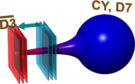
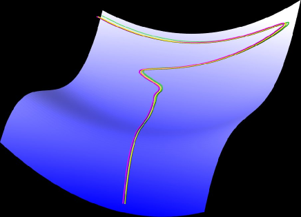
Figure 1: Brane setup and field trajectories. The potential features a local minimum for the volume modulus and an inflection point for the inflaton, the brane-anti-brane separation.

The stabilization of the volume modulus is done by $D7$ branes spanning the 3 large space dimensions and wrapping four-cycles of the compact space. Gaugino condensation in the stacks of wrapped $D7$ branes generates a non-trivial superpotential for the volume modulus, which in the simplest case takes the form given in Kachru:2003aw .

$$W=w_{0}+Ae^{-iaT}$$ (1)

The non-trivial embedding of the $D7$ branes in the compact space makes the coefficient $A$ dependent on the position of the mobile $D3$ brane Baumann:2006th . An additional dependence of the scalar potential derived from Eq.(1) on the position of the mobile brane comes from the non-trivial Kähler metric 5. The resulting effects of the moduli stabilization and the uplifting of the vacuum from anti-deSitter to deSitter by adding anti-$D3$ branes give a potential that is generally too steep for inflation, the value of the slow-roll parameter $\eta$ being $\eta=2/3$ Kachru:2003sx . However, when taking into account the competing effects of the moduli stabilization and anti-brane attraction, the resulting potential for the mobile brane features an inflection point Burgess:2004kv ; Cline:2005ty ; Baumann:2007np . The vanishing of the $\eta$ parameter at this point makes it possible for inflation to work, most of the $e$-folds coming from a small region of field space.

Apriori, such models require a large amount of fine-tuning, as the slope of the potential, and therefore the $\epsilon$ slow-roll parameter, at the inflection point must be very small. However, multi-brane models offer the possibility to alleviate this fine-tuning via the dynamical flattening mechanism for the inflaton potential. In what follows we will study the cosmological signatures of multi-brane models going beyond the calculations of amplitude of the density perturbations, the spectral index and it running to determine what unique signatures one can expect to be detectable in cosmological observations.

II.1 The Kähler potential

The Kähler potential proposed by DeWolfe and Giddings DeWolfe:2002nn has the following form:

$${\mathcal{K}}=-3\log\left(r\right)=-3\log\left(T+\overline{T}-f\left(\varphi^{i},\overline{\varphi}^{i}\right)\right),$$ (2)

where we will assume that for a multi-brane setup the function $f$ decomposes on a sum of functions, each one depending on one brane position $\varphi^{i}$:

$${\mathcal{K}}=-3\log\left(T+\overline{T}-\sum_{i}f_{i}\left(\varphi^{i},\overline{\varphi}^{i}\right)\right).$$ (3)

The calculations in this paper use the simplest form of the functions $f_{i}$:

$$f_{i}\left(\varphi^{i},\overline{\varphi}^{i}\right)=\varphi^{i}\overline{\varphi}^{i}.$$ (4)

One can justify this assumption by taking into account the fact that most $e$-folds of inflation are produced around the inflection point of the potential and therefore the functions $f_{i}$ can be expanded to the lowest order in the brane positions.

In the general case the Kähler metric derived from the Kähler potential of Eq.(3) has the form:

$${\mathcal{K}}_{a\overline{b}}=\frac{3}{r^{2}}\left(\begin{array}[]{ccccc}1&-\frac{\partial f_{1}}{\partial\varphi_{1}}&-\frac{\partial f_{2}}{\partial\varphi_{2}}&\cdots&-\frac{\partial f_{n}}{\partial\varphi_{n}}\\ -\frac{\partial f_{1}}{\partial\varphi_{1}^{*}}&\frac{\partial f_{1}}{\partial\varphi_{1}}\frac{\partial f_{1}}{\partial\varphi_{1}^{*}}+r\frac{\partial^{2}f_{1}}{\partial\varphi_{1}\partial\varphi_{1}^{*}}&\frac{\partial f_{1}}{\partial\varphi_{1}^{*}}\frac{\partial f_{2}}{\partial\varphi_{2}}&\cdots&\frac{\partial f_{1}}{\partial\varphi_{1}^{*}}\frac{\partial f_{n}}{\partial\varphi_{n}}\\ \vdots&\vdots&\vdots&\ddots&\vdots\\ -\frac{\partial f_{n-1}}{\partial\varphi_{n-1}^{*}}&\frac{\partial f_{n-1}}{\partial\varphi_{n-1}^{*}}\frac{\partial f_{1}}{\partial\varphi_{1}}&\frac{\partial f_{n-1}}{\partial\varphi_{n-1}^{*}}\frac{\partial f_{2}}{\partial\varphi_{2}}&\cdots&\frac{\partial f_{n-1}}{\partial\varphi_{n-1}^{*}}\frac{\partial f_{n}}{\partial\varphi_{n}}\\ -\frac{\partial f_{n}}{\partial\varphi_{n}^{*}}&\frac{\partial f_{n}}{\partial\varphi_{n}^{*}}\frac{\partial f_{1}}{\partial\varphi_{1}}&\frac{\partial f_{n}}{\partial\varphi_{n}^{*}}\frac{\partial f_{2}}{\partial\varphi_{2}}&\cdots&\frac{\partial f_{n}}{\partial\varphi_{n}^{*}}\frac{\partial f_{n}}{\partial\varphi_{n}}+r\frac{\partial^{2}f_{n}}{\partial\varphi_{n}\partial\varphi_{n}^{*}}\end{array}\right)$$ (5)

The inverse can also be calculated in the general case (see appendix A.1). We want to write the kinetic energy in terms of the real and imaginary parts of the fields Burgess:2004kv . The imaginary parts will play no role in our subsequent analysis as they will roll very quickly to their respective minima and these minima do not shift during the rolling of the real parts Kallosh:2004yh . We write the volume modulus as $T=\sigma+{\mathbbm{i}}\omega$ and the brane positions as $\varphi^{i}=\phi^{i}+{\mathbbm{i}}\chi^{i}$ which allows us to read off the field space metric and it inverse for the $\sigma$ and $\phi^{i}$ fields:

$$G_{ij}=\frac{6}{r^{2}}\left(\begin{array}[]{cc}1&-\phi^{i}\\ -\phi^{i}&r\delta_{ij}+\phi^{i}\phi^{j}\end{array}\right)\;\;,\;\;\;\;G^{ij}=\frac{r}{6}\left(\begin{array}[]{cc}2\sigma&\phi^{i}\\ \phi^{i}&\delta_{ij}\end{array}\right)$$ (6)

II.2 The potential

In this section we describe the various contributions to the scalar potential. They are the F-term responsible for the stabilization of the volume modulus, the anti-brane contribution that uplifts the resulting anti-deSitter minimum to a deSitter one, and the brane-anti-brane attractive potential which gives a non-trivial evolution to the inflatons. The F-term is calculated with the usual formula:

$$V_{F}=e^{\mathcal{K}}\left(K^{\overline{a}b}\overline{D_{a}W}D_{b}W-3\left|W\right|^{2}\right),$$ (7)

where ${\mathcal{K}}$ is given in Eq. (3). Let us take for example a scenario with two mobile branes; the Kähler potential is:

$$K=-3\log\left(r\right)=-3\log\left(T+\overline{T}-f_{1}\left(\phi^{1},\overline{\phi^{1}}\right)-f_{2}\left(\phi^{2},\overline{\phi^{2}}\right)\right).$$ (8)

We take the superpotential to be the racetrack one, this way the vacuum with no anti-brane present is already Minkowski Kallosh:2004yh :

$$W=w_{0}+Ae^{-aT}+Be^{-bT}.$$ (9)

If we take the minimal form for the functions $f_{1}\left(\phi^{1},\overline{\phi^{1}}\right)$ and $f_{2}\left(\phi^{2},\overline{\phi^{2}}\right)$ and the general expression for the F-term, Eq. (73), the resulting potential has a very simple form:

$$V_{F} = \frac{e^{-a\sigma}}{3r^{2}}\left[aA^{2}e^{-a\sigma}\left(3+a\sigma\right)+aAw_{0}\cos\left(a\omega\right)\right]+$$ (10)

$$\frac{e^{-b\sigma}}{3r^{2}}\left[bB^{2}e^{-b\sigma}\left(3+b\sigma\right)+bBw_{0}\cos\left(b\omega\right)\right]+$$

$$\frac{ABe^{-\left(a+b\right)\sigma}}{3r^{2}}\left[3\left(a+b\right)+2ab\sigma\right]\cos\left(\left(a-b\right)\omega\right)$$

The minimal form of the functions $f_{1}$ and $f_{2}$ brings an important simplification as the dependence of the F-term potential on the positions of the mobile branes comes only through $r=T+\overline{T}-\phi^{1}\overline{\phi^{1}}-\phi^{2}\overline{\phi^{2}}$.

The anti-branes that lift the minimum of the potential to a deSitter one during inflation have a contribution of the form:

$$V_{sb}=\sum_{i=1}^{N}\frac{E_{i}}{r^{\alpha}}.$$ (11)

The coefficients $E_{i}$ are the warped anti-brane tension. The exponent $\alpha=2$ for anti-branes located in a highly warped region, i.e. at the bottom of the throat Kachru:2003sx . It is not necessary that all branes are located inside the same throat Iizuka:2004ct , but we will consider a single-throat model for simplicity.

We also have to add the Newtonian attractive pieces for the branes and anti-branes:

$$V_{N}=-\sum_{i=1,j=1}^{M,N}\frac{k_{ij}}{r^{2}\left(\phi^{i}-\phi_{0}^{j}\right)^{4}}.$$ (12)

We want to trace the evolution of more than one brane, and the above potential is singular when an brane collides with an anti-brane. Therefore we want to regulate the Newtonian potential such that it reproduces the correct inverse-power-law at large distances, but at the same time is regular and cancels the brane-anti-brane tension at zero separation. We follow here the method of Ref. Cline:2005ty and for a given brane-anti-brane pair we choose

$$V_{N}\left(\phi^{i}\right)=-\sum_{i=1,j=1}^{M,N}\frac{k_{ij}}{r^{2}\left[s^{ij}+\left(\phi^{i}-\phi_{0}^{j}\right)^{4}\right]},$$ (13)

where the constant $s^{ij}$ is chosen such that when $\phi^{i}=\phi_{0}^{j}$, the Newtonian potential exactly cancels the contribution to the potential of the anti-brane placed at $\phi_{0}^{j}$. If there are more than one anti-brane located at $\phi_{0}^{j}$, we choose $s^{ij}$ to cancel the tension of only one of them.

To summarise, the choice of Kähler potential and the assumption that we have a single-throat model, such that all anti-branes are located at the same point, allows us to write the scalar potential for a model with $n$ mobile branes and $n$ anti-branes as:

$$V\left(\sigma,\phi^{1}\dots\phi^{n}\right)=\frac{V_{0}}{r^{2}}\left[F\left(\sigma\right)+nT-\sum_{i=1}^{n}\frac{nk}{s^{i}+\left(\phi^{i}-\phi_{0}\right)^{4}}\right].$$ (14)

The function $F\left(\sigma\right)$ contributed by the F-term is responsible for the stabilisation of the volume modulus at some value $\sigma_{0}$, and, as long as we do not add too many anti-branes to destabilise this minimum, we can simply approximate $F\left(\sigma\right)=\frac{1}{2}m_{\sigma}^{2}\left(\sigma-\sigma_{0}\right)^{2}$ when studying the cosmological signatures of the model.

III Properties of the field space metric

We want to get a better understanding of the properties of the target (field) space. In order to do so we would like to write the Kähler metric for the real parts of the fields in a more convenient coordinate system.

$$dS^{2} = \frac{6}{r^{2}}\left[d\sigma^{2}-2\phi^{i}d\phi^{i}d\sigma+rd\phi^{i}d\phi^{i}+\phi^{i}\phi^{j}d\phi^{i}d\phi^{j}\right]=$$ (15)

$$\frac{6}{r^{2}}\left[\left(d\sigma-\phi^{i}d\phi^{i}\right)^{2}+rd\phi^{i}d\phi^{i}\right]=\frac{6}{r^{2}}\left[\frac{1}{4}dr^{2}+rd\phi^{i}d\phi^{i}\right]$$

We can now redefine the coordinate $r$ as $r=u^{2}$. This brings the metric in the form:

$$dS^{2}=\frac{6}{u^{4}}\left[\frac{4u^{2}du^{2}}{4}+u^{2}d\phi^{i}d\phi^{i}\right]=\frac{6}{u^{2}}\left[du^{2}+\sum_{i=1}^{n}{d\phi^{i}}^{2}\right],$$ (16)

which is the metric for the $n+1$ - dimensional Euclidean AdS space. The original coordinates cover only a limited patch of the space, the boundary of it being given by the condition:

$$2\sigma-\sum_{i=1}^{n}{\phi^{i}}^{2}>0,$$ (17)

which translates into the condition that $u>0$. This is the Poincaré half-space model of AdS, Caldarelli:1998wk . The expressions for the metric connection coefficients are much simpler in the new variable. Up to symmetries in permuting the indices:

$$\Gamma^{u}_{~{}uu} = -\frac{1}{u}$$

$$\Gamma^{u}_{~{}ij} = \frac{\delta_{ij}}{u}$$

$$\Gamma^{i}_{~{}uj} = -\frac{\delta_{ij}}{u}$$

All other connection coefficients, most notably $\Gamma^{i}_{~{}jk}$ vanish and the non-vanishing ones are now independent of the brane positions. As far as the potential of the effective theory is concerned, one has to replace $\sigma$ by the new variable $u$:

$$r=2\sigma-\sum_{i=1}^{n}{\phi^{i}}^{2}=u^{2},~{}~{}~{}\sigma=\frac{1}{2}\left(u^{2}+\sum_{i=1}^{n}{\phi^{i}}^{2}\right).$$ (19)

In KKLT type of models the potential has the form Eq. (14), this change of variables brings the potential to the form:

$$V\left(u,\phi^{1}\dots\phi^{n}\right)=\frac{V_{0}}{u^{4}}\left[F\left(\frac{u^{2}}{2}+\frac{1}{2}\sum_{i=1}^{n}{\phi^{i}}^{2}\right)+nT-\sum_{i=1}^{n}\frac{nk}{\left(\phi^{i}-\phi_{0}\right)^{4}}\right].$$ (20)

The volume-stabilising function $F$ preserves the full $SO\left(n\right)$ rotational symmetry of the brane-position inflatons, and the dependence on the brane positions is removed from the overall factor $1/u^{4}$. Combined with the fact that in terms of the new variables the field-space metric is independent of the positions of the branes, the Newtonian brane-anti-brane attraction remains the only part of the potential which sets a preferred direction in the field space. This will lead to a field trajectory during slow roll that will be a straight line, and therefore to very small signatures in the CMB power spectrum.

IV Field evolution and inflation

To study the dynamics of the fields during inflation we start with the action for the scalar fields coupled to gravity:

$$S=\int d^{3}xdt\sqrt{-g}\left(-\frac{1}{2}G_{ij}\partial_{\mu}\phi^{i}\partial^{\mu}\phi^{j}-V+\frac{R}{16\pi G}\right).$$ (21)

We assume that the space-time metric is of the FRW type,

$$ds^{2}=-dt^{2}+a^{2}\left(t\right)\left(dr^{2}+r^{2}d\Omega^{2}\right),$$ (22)

and we decompose the fields into a background, homogeneous part, and a space-dependent perturbation. The equation for the homogeneous fields is the geodesic equation in field space with a driving force given by the potential gradient and a damping force given by Hubble expansion:

$$\ddot{\phi}^{k}+3H\dot{\phi}^{k}+G^{ka}\frac{\partial V}{\partial\phi^{a}}+\Gamma_{ij}^{k}\dot{\phi}^{i}\dot{\phi}^{j}=0.$$ (23)

The Hubble constant and its time derivative are given by:

$$H^{2}=\frac{8\pi G}{3}\left(\frac{1}{2}G_{ij}\dot{\phi}^{i}\dot{\phi}^{j}+V\right)\;\;,\;\;\;\dot{H}=-(4\pi G)G_{ij}\dot{\phi}^{i}\dot{\phi}^{j}.$$ (24)

We write here the more general equation for inhomogeneous fields, as we will need it later when studying the perturbations around the homogeneous background:

$$\frac{1}{\sqrt{-g}}\partial_{\mu}\left[\sqrt{-g}g^{\mu\nu}\partial_{\nu}\phi^{K}\right]-G^{KA}\frac{\partial V}{\partial\phi^{A}}+\Gamma_{IJ}^{K}g^{\mu\nu}\partial_{\mu}\phi^{I}\partial_{\nu}\phi^{J}=0$$ (25)

$$H^{2}=\frac{1}{3}\left(G_{IJ}g^{\mu\nu}\partial_{\mu}\phi^{I}\partial_{\nu}\phi^{J}+V\right)$$ (26)

V Perturbation equations

In this section we analyze the perturbations around the background, slow-roll evolution. First, the background fields and metric are only dependent on time, while the perturbations are dependent on space as well. We will follow Ref.Gordon:2000hv and parametrise the metric perturbations as follows:

$$g_{\mu\nu}+\delta g_{\mu\nu}=\left(\begin{array}[]{cc}-\left(1+2A\left(t,{\bf x}\right)\right)&a\left(t\right)B_{,i}\left(t,{\bf x}\right)\\ a\left(t\right)B_{,i}\left(t,{\bf x}\right)&a^{2}\left(t\right)\left[\left(1-2\psi\left(t,{\bf x}\right)\right)\delta_{ij}+2E_{,ij}\left(t,{\bf x}\right)\right],\end{array}\right)$$ (27)

and that of the fields $\phi^{I}$ as:

$$\phi^{I}=\phi^{I}\left(t\right)+\delta\phi^{I}\left(t,{\bf x}\right).$$ (28)

We now expand the evolution equation (23) for the fields $\phi^{I}$ around the background. We will look at each term in the equation separately.

V.1 Kinetic Term

We start with the first term in Eq.(25) and write the scalars and the metric as in Eq.(27,28). The result for the plane wave expanded perturbations (see appendix A.2 for details) is:

$$\delta\left(\frac{1}{\sqrt{-g}}\partial_{\mu}\left[\sqrt{-g}g^{\mu\nu}\partial_{\nu}\phi^{K}\right]\right)=-\ddot{\delta\phi^{K}}-3\frac{\dot{a}}{a}\dot{\delta\phi^{K}}-\frac{k^{2}}{a^{2}}\delta\phi^{K}$$

$$+2A\left[\ddot{\phi^{K}}+3\frac{\dot{a}}{a}\dot{\phi^{K}}+\Gamma_{IJ}^{K}\dot{\phi^{I}}\dot{\phi^{J}}\right]+2\dot{A}\dot{\phi^{K}}-\frac{k^{2}}{a}B\dot{\phi^{K}}-\left[\dot{A}-3\dot{\psi}-k^{2}\dot{E}\right]\dot{\phi^{K}},$$ (29)

where $k\equiv|{\vec{k}}|$ is the expansion wavenumber.

V.2 Potential and Christoffel Terms

The perturbation of the potential term is the simplest one, since it does not involve the space-time metric. We simply take the variation with respect to the fields $\phi^{I}$ :

$$\delta\left(G^{KI}\frac{\partial V}{\partial\phi^{I}}\right)=\left[G^{KI}\frac{\partial^{2}V}{\partial\phi^{I}\partial\phi^{J}}+\frac{\partial G^{KI}}{\partial\phi^{J}}\frac{\partial V}{\partial\phi^{I}}\right]\delta\phi^{J}.$$ (30)

Finally, we have to calculate the perturbation of the connection coefficients coming from the non-trivial field-space metric. They are:

$$\Gamma_{IJ}^{K}\left(\phi+\delta\phi\right)g^{\mu\nu}\partial_{\mu}\left(\phi^{I}+\delta\phi^{I}\right)\partial_{\nu}\left(\phi^{J}+\delta\phi^{J}\right)=\underbrace{\Gamma_{IJ}^{K}g^{\mu\nu}\partial_{\mu}\phi^{I}\partial_{\nu}\phi^{J}}_{\text{background}}$$

$$+2\Gamma_{IJ}^{K}g^{\mu\nu}\partial_{\mu}\phi^{I}\partial_{\nu}\delta\phi^{J}+\frac{\partial\Gamma_{IJ}^{K}}{\partial\phi^{L}}g^{\mu\nu}\partial_{\mu}\phi^{I}\partial_{\nu}\phi^{J}\delta\phi^{L}+\Gamma_{IJ}^{K}\delta g^{\mu\nu}\partial_{\mu}\phi^{I}\partial_{\nu}\phi^{J}=$$

$$\underbrace{\Gamma_{IJ}^{K}g^{\mu\nu}\partial_{\mu}\phi^{I}\partial_{\nu}\phi^{J}}_{\text{background}}-2\Gamma_{IJ}^{K}\dot{\phi^{I}}\dot{\delta\phi^{J}}-\frac{\partial\Gamma_{IJ}^{K}}{\partial\phi^{L}}\dot{\phi^{I}}\dot{\phi^{J}}\delta\phi^{L}+2A\Gamma_{IJ}^{K}\dot{\phi^{I}}\dot{\phi^{J}}$$ (31)

We can now collect the perturbation terms and write the equation for the fluctuations of the fields:

$$-\ddot{\delta\phi^{K}}-3\frac{\dot{a}}{a}\dot{\delta\phi^{K}}-\frac{k^{2}}{a^{2}}\delta\phi^{K}+2A\underbrace{\left[\ddot{\phi^{K}}+3\frac{\dot{a}}{a}\dot{\phi^{K}}+\Gamma_{IJ}^{K}\dot{\phi^{I}}\dot{\phi^{J}}\right]}_{=-2AG^{KI}\frac{\partial V}{\partial\phi^{I}}}+2\dot{A}\dot{\phi^{K}}-\frac{k^{2}}{a}B\dot{\phi^{K}}$$

$$-\left[\dot{A}-3\dot{\psi}-k^{2}\dot{E}\right]\dot{\phi^{K}}-\left[G^{KI}\frac{\partial^{2}V}{\partial\phi^{I}\partial\phi^{J}}+\frac{\partial G^{KI}}{\partial\phi^{J}}\frac{\partial V}{\partial\phi^{I}}\right]\delta\phi^{J}$$

$$-2\Gamma_{IJ}^{K}\dot{\phi^{I}}\dot{\delta\phi^{J}}-\frac{\partial\Gamma_{IJ}^{K}}{\partial\phi^{L}}\dot{\phi^{I}}\dot{\phi^{J}}\delta\phi^{L}=0$$ (32)

Using the equation for the background fields, the perturbation equation can be rewritten as:

$$\ddot{\delta\phi^{K}}+3\frac{\dot{a}}{a}\dot{\delta\phi^{K}}+\frac{k^{2}}{a^{2}}\delta\phi^{K}+\left[G^{KI}\frac{\partial^{2}V}{\partial\phi^{I}\partial\phi^{J}}+\frac{\partial G^{KI}}{\partial\phi^{J}}\frac{\partial V}{\partial\phi^{I}}\right]\delta\phi^{J}$$

$$=-2AG^{KI}\frac{\partial V}{\partial\phi^{I}}+\left[\dot{A}+3\dot{\psi}+k^{2}\dot{E}-\frac{k^{2}}{a}B\right]\dot{\phi^{K}}$$

$$-2\Gamma_{IJ}^{K}\dot{\phi^{I}}\dot{\delta\phi^{J}}-\frac{\partial\Gamma_{IJ}^{K}}{\partial\phi^{L}}\dot{\phi^{I}}\dot{\phi^{J}}\delta\phi^{L}=0$$ (33)

VI Metric Perturbations

In this section we analyse the perturbations of the Einstein equations, namely the perturbations of the Einstein tensor and stress-energy tensor. We start with the parametrisation of the metric perturbations given in Eq. (27):

$$\delta g_{\mu\nu}=\left(\begin{array}[]{cccc}-2A&aB_{,1}&aB_{,2}&aB_{,3}\\ aB_{,1}&2a^{2}\left(-2\psi+E_{,11}\right)&2a^{2}E_{,12}&2a^{2}E_{,13}\\ aB_{,2}&2a^{2}E_{,21}&2a^{2}\left(-2\psi+E_{,22}\right)&2a^{2}E_{,23}\\ aB_{,3}&2a^{2}E_{,31}&2a^{2}E_{,32}&2a^{2}\left(-2\psi+E_{,33}\right)\\ \end{array}\right).$$ (34)

The functions $A$, $\psi$, $B$, and $E$ are in general dependent upon all coordinates, $t,x,y,z$. We follow here Ref. Mukhanov:1990me and perturb the Einstein equations written in the form:

$$R_{\mu}^{\nu}-\frac{1}{2}R\delta_{\mu}^{\nu}=8\pi GT_{\mu}^{\nu}.$$ (35)

First, the perturbations of the Einstein tensor is:

$$\delta\left(R_{0}^{0}-\frac{1}{2}R\delta_{0}^{0}\right) = 6\frac{\dot{a}}{a}\left(\frac{\dot{a}}{a}A+\dot{\psi}\right)+2\frac{k^{2}}{a^{2}}\left[\psi+\frac{\dot{a}}{a}\left(a^{2}\dot{E}-aB\right)\right]$$ (36)

$$\delta R_{0}^{i} = 2\left(\dot{\psi}+\frac{\dot{a}}{a}A\right)_{,i}$$ (37)

For the stress-energy tensor the general expression is:

$$T_{\alpha}^{\beta}=-\left[\frac{1}{2}G_{IJ}g^{\mu\nu}\partial_{\mu}\phi^{I}\partial_{\nu}\phi^{J}+V\right]\delta_{\alpha}^{\beta}+G_{IJ}\partial_{\alpha}\phi^{I}\partial^{\beta}\phi^{J}.$$ (38)

We now perturb the stress-energy tensor according to our parametrisation of the metric and field perturbations we obtain:

$$\delta T_{\alpha}^{\beta}=-\left[\frac{1}{2}G_{IJ}\delta g^{\mu\nu}\partial_{\mu}\phi^{I}\partial_{\nu}\phi^{J}+G_{IJ}g^{\mu\nu}\partial_{\mu}\phi^{I}\partial_{\nu}\delta\phi^{J}\right.$$

$$\left.+\frac{1}{2}\frac{\partial G_{IJ}}{\partial\phi^{K}}g^{\mu\nu}\partial_{\mu}\phi^{I}\partial_{\nu}\phi^{J}\delta\phi^{K}+\frac{\partial V}{\partial\phi^{K}}\delta\phi^{K}\right]\delta_{\alpha}^{\beta}$$

$$+G_{IJ}(\partial_{\alpha}\delta\phi^{I}\partial_{\gamma}\phi^{J}+\partial_{\alpha}\phi^{I}\partial_{\gamma}\delta\phi^{J})g^{\gamma\beta}$$

$$+\frac{G_{IJ}}{\partial\phi^{K}}\partial_{\alpha}\phi^{I}\partial^{\beta}\phi^{J}\delta\phi^{K}+G_{IJ}\partial_{\alpha}\phi^{I}\partial_{\gamma}\phi^{J}\delta g^{\gamma\beta}$$ (39)

We can use here the fact that the background fields are homogeneous to further simplify the expression for $\delta T_{0}^{0}$. We obtain:

$$\delta T_{0}^{0}=\left[-\frac{1}{2}G_{IJ}\delta g^{00}\dot{\phi^{I}}\dot{\phi^{J}}+G_{IJ}\dot{\phi^{I}}\dot{\delta\phi^{J}}+\frac{1}{2}\frac{\partial G_{IJ}}{\partial\phi^{K}}\dot{\phi^{I}}\dot{\phi^{J}}\delta\phi^{K}-\frac{\partial V}{\partial\phi^{K}}\delta\phi^{K}\right]\delta_{0}^{0}$$

$$-\frac{\partial G_{IJ}}{\partial\phi^{K}}\dot{\phi^{I}}\dot{\phi^{J}}\delta\phi^{K}-2G_{IJ}\dot{\phi^{I}}\dot{\delta\phi^{J}}+G_{IJ}\dot{\phi^{I}}\dot{\phi^{J}}\delta g^{00}=$$

$$AG_{IJ}\dot{\phi^{I}}\dot{\phi^{J}}-G_{IJ}\dot{\phi^{I}}\dot{\delta\phi^{J}}-\frac{1}{2}\frac{\partial G_{IJ}}{\partial\phi^{K}}\dot{\phi^{I}}\dot{\phi^{J}}\delta\phi^{K}-\frac{\partial V}{\partial\phi^{K}}\delta\phi^{K}$$ (40)

For the component $T_{0}^{i}$ the background value is trivial, $T_{0}^{i}=0$ and the only term that contributes is the one in the next-to-last line in Eq.(39):

$$\delta T_{0}^{i}=G_{IJ}\dot{\phi^{I}}\partial_{i}\delta\phi^{J}.$$ (41)

Therefore the equation for the evolution of the metric perturbations become:

$$2\left(\dot{\psi}+\frac{\dot{a}}{a}A\right)_{,i}=8\pi G\cdot G_{IJ}\dot{\phi^{I}}\delta\phi^{J}_{,i}$$ (42)

$$6\frac{\dot{a}}{a}\left(\frac{\dot{a}}{a}A+\dot{\psi}\right)+2\frac{k^{2}}{a^{2}}\left[\psi+\frac{\dot{a}}{a}\left(a^{2}\dot{E}-aB\right)\right]=$$

$$8\pi G\left[AG_{IJ}\dot{\phi^{I}}\dot{\phi^{J}}-G_{IJ}\dot{\phi^{I}}\dot{\delta\phi^{J}}-\frac{1}{2}\frac{\partial G_{IJ}}{\partial\phi^{K}}\dot{\phi^{I}}\dot{\phi^{J}}\delta\phi^{K}-\frac{\partial V}{\partial\phi^{K}}\delta\phi^{K}\right]$$ (43)

VII The evolution and spectrum of the perturbations

We now proceed to deriving the equation of motion for the gauge-invariant Mukhanov-Sasaki variables

$$Q^{I}=\delta\phi^{I}+\frac{\dot{\phi^{I}}}{H}\psi.$$ (44)

For the single field, slow-roll case the equations of motions for the variable $a\,Q$ assume a particularly simple form of an oscillator with a time (background only) dependent mass. The perturbations in the scalar sector are then easily integrated from an initial state which can be approximated by a Minkowski adiabatic vacuum for $k\gg aH$ to a final state at horizon crossing $k=aH$ after which the perturbation freezes out and stops evolving.

For multiple field models two complications can arise. The first is that mixing terms in the multiple field potential will lead to a system of coupled oscillators with a non-diagonal mass matrix. The second is that a non-trivial field-space metric (kinetic terms) leads to the presence of connection terms in the equations. Another important difference with the single field case is that, in general, the perturbations will continue evolving once they cross the horizon and must be solved for well into the super-horizon regime.

In what follows we use the spatially flat gauge in which

$$\psi_{Q} = 0,$$ (45)

$$a^{2}\dot{E}_{Q}-aB_{Q} = \frac{1}{H}\Psi,$$ (46)

where the subscript $Q$ denotes the use of the spatially flat gauge and $\Psi$ is the curvature perturbation. This gauge makes the equations simple as the Mukhanov-Sasaki variables reduce to the simple form:

$$Q^{I}=\delta\phi^{I}.$$ (47)

Introducing the choice of gauge into Eq. (42) leads the to following expression for $A_{Q}$:

$$A_{Q}=\left(\frac{4\pi G}{H}\right)G_{IJ}\dot{\phi^{I}}\delta\phi^{J}.$$ (48)

Differentiating this we then obtain

$$\dot{A}_{Q}=\left(\frac{4\pi G}{H}\right)\left[-\frac{\dot{H}}{H}G_{IJ}\dot{\phi}^{I}\delta\phi^{J}+\frac{\partial G_{IJ}}{\partial\phi^{K}}\dot{\phi^{I}}\delta{\phi^{J}}\dot{\phi}^{K}+G_{I}J\ddot{\phi}^{I}\delta\phi^{J}+G_{I}J\dot{\phi}^{I}\dot{\delta\phi^{J}}\right].$$ (49)

The value for $\Psi$ comes from Equation (43):

$$3H^{2}A_{Q}+\frac{k^{2}}{a^{2}}\Psi=4\pi G\left[A_{Q}G_{IJ}\dot{\phi^{I}}\dot{\phi^{J}}-G_{IJ}\dot{\phi^{I}}\dot{\delta\phi^{J}}-\frac{1}{2}\frac{\partial G_{IJ}}{\partial\phi^{K}}\dot{\phi^{I}}\dot{\phi^{J}}\delta\phi^{K}-\frac{\partial V}{\partial\phi^{K}}\delta\phi^{K}\right].$$ (50)

Thus the curvature perturbation has the expression:

$$\frac{1}{H}\frac{k^{2}}{a^{2}}\Psi = \left(\frac{4\pi G}{H}\right)\left[-3HG_{IJ}\dot{\phi}^{I}\delta\phi^{J}+\left(\frac{4\pi G}{H}\right)G_{LM}\dot{\phi^{L}}\dot{\phi^{M}}G_{IJ}\dot{\phi^{I}}\delta\phi^{J}\right.$$ (51)

$$\left.-G_{IJ}\dot{\phi^{I}}\dot{\delta\phi^{J}}-\frac{1}{2}\frac{\partial G_{IJ}}{\partial\phi^{K}}\dot{\phi^{I}}\dot{\phi^{J}}\delta\phi^{K}-\frac{\partial V}{\partial\phi^{K}}\right]\delta\phi^{K}.$$

Using the previously-derived expressions for $A_{Q}$ and $\Phi$ we can now calculate the gauge terms in the right-hand-side of the equations of motion of the perturbation variables, Equation (33).

$$-2AG^{KI}\frac{\partial V}{\partial\phi^{I}} + \left[\dot{A}+3\dot{\psi}+k^{2}\dot{E}-\frac{k^{2}}{a}B\right]\dot{\phi^{K}}=-2A_{Q}G^{KI}\frac{\partial V}{\partial\phi^{I}}+\left[\dot{A_{Q}}+\frac{1}{H}\frac{k^{2}}{a^{2}}\Psi\right]\dot{\phi^{K}}$$ (52)

$$= \left(\frac{8\pi G}{H}\right)\left[G_{IJ}\ddot{\phi}^{K}\dot{\phi}^{I}\delta\phi^{J}+3HG_{IJ}\dot{\phi}^{K}\dot{\phi}^{I}\delta\phi^{J}+\Gamma_{ILJ}\dot{\phi}^{K}\dot{\phi}^{I}\dot{\phi}^{L}\delta\phi^{J}\right.$$

$$\left.+G_{IJ}\dot{\phi}^{K}\ddot{\phi}^{I}\delta\phi^{J}-\frac{\dot{H}}{H}G_{IJ}\dot{\phi}^{K}\dot{\phi}^{I}\delta\phi^{J}\right]$$

$$= \left[\left(\frac{8\pi G}{a^{3}}\right)G_{IJ}\frac{\partial}{\partial t}\left(\frac{a^{3}\dot{\phi}^{K}\dot{\phi}^{I}}{H}\right)+\left(\frac{8\pi G}{H}\right)\Gamma_{ILJ}\dot{\phi}^{K}\dot{\phi}^{I}\dot{\phi}^{L}\right]\delta\phi^{J}$$

Now we combine all the above results, Equations (49), (51), and (52) can now be combined to rewrite the equation of motion for each perturbation $\delta\phi^{I}$, Eq. (33), in terms of the new variable $Q^{I}$

$$\ddot{Q^{K}}+3H\dot{Q^{K}}+\frac{k^{2}}{a^{2}}Q^{K}+2\Gamma_{IJ}^{K}\dot{\phi^{I}}\dot{Q^{J}}+\left[G^{KI}\frac{\partial^{2}V}{\partial\phi^{I}\partial\phi^{J}}\right.$$

$$+\frac{\partial G^{KI}}{\partial\phi^{J}}\frac{\partial V}{\partial\phi^{I}}+\frac{\partial\Gamma_{IJ}^{K}}{\partial\phi^{L}}\dot{\phi^{I}}\dot{\phi^{J}}\dot{\phi}^{L}-\left(\frac{8\pi G}{a^{3}}\right)G_{IJ}\frac{\partial}{\partial t}\left(\frac{a^{3}\dot{\phi}^{K}\dot{\phi}^{I}}{H}\right)$$

$$\left.-\left(\frac{8\pi G}{H}\right)\Gamma_{ILJ}\dot{\phi}^{K}\dot{\phi}^{I}\dot{\phi}^{L}-\left(\frac{8\pi G}{H}\right)\Gamma^{K}_{LM}\dot{\phi}^{L}\dot{\phi}^{M}G_{IJ}\dot{\phi}^{I}\right]Q^{J}=0.$$ (53)

Notice that all coefficients in the equation above depend only on background quantities. For a canonical kinetic term, $G_{IJ}=\delta_{ij}$, all the connection coefficients vanish and the only mixing of the Mukhanov-Sasaki variables $Q^{K}$ comes from the mass matrix of the inflatons. The mixing provided by the non-trivial field-space metric enhances the possibility that non-trivial features on the power spectrum can be detectable.

VII.1 Adiabatic and Entropy Perturbations

Equation (VII) allows one to integrate efficiently the system of perturbations from an initial state well inside the horizon to a final, super-horizon state at the end of inflation when the perturbations determine initial conditions in the constituents of the universe after a period of preheating.

In the single field scenario the perturbations in the inflaton are simply related to perturbations in the curvature. If multiple fields are present however there can exist entropy perturbations between the different fields which leave the curvature unperturbed. The two types of perturbations induce different initial conditions for the fluid perturbations at the beginning of the radiation era and lead to different CMB signatures cmbisocurv .

In terms of the generalized trajectory for the variables $Q^{K}$ one can define a single adiabatic (or curvature) and $n-1$ entropy perturbations at any point along the trajectory. The decomposition allows one to identify the observationally distinct perturbations at the end of inflation. The variables $Q^{K}$ define a “perturbation vector”, $\overrightarrow{Q}$ in field space. We can decompose this vector in two components: the one parallel to the velocity of the background fields and the component orthogonal to it. We start by defining the unit field velocity vector, or the adiabatic direction.

$$\overrightarrow{a}=\frac{\dot{\phi^{i}}}{\sqrt{G_{kl}\dot{\phi}^{k}\dot{\phi}^{l}}}.$$ (54)

The adiabatic perturbation is defined by projecting the perturbation vector $\overrightarrow{Q}$ along the adiabatic direction $\overrightarrow{a}$.

$$Q_{\sigma}=\frac{G_{ij}\dot{\phi^{i}}Q^{j}}{\sqrt{G_{kl}\dot{\phi}^{k}\dot{\phi}^{l}}}=\frac{\dot{\phi^{i}}\delta\phi^{j}}{\sqrt{G_{kl}\dot{\phi}^{k}\dot{\phi}^{l}}}+\frac{\sqrt{G_{kl}\dot{\phi}^{k}\dot{\phi}^{l}}}{H}\psi.$$ (55)

The corresponding entropy direction is defined as the component of $\overrightarrow{Q}$ orthogonal to $\overrightarrow{a}$:

$$\overrightarrow{e}=\frac{\overrightarrow{Q}-\left(\overrightarrow{a}\cdot\overrightarrow{Q}\right)\overrightarrow{a}}{\left|\overrightarrow{Q}-(\overrightarrow{a}\cdot\overrightarrow{Q})\overrightarrow{a}\right|}.$$ (56)

The entropy perturbation is the projection of $\overrightarrow{Q}$ along $\overrightarrow{e}$:

$$Q_{s}=\frac{\left|\overrightarrow{Q}\right|^{2}-\left(\overrightarrow{a}\cdot\overrightarrow{Q}\right)^{2}}{\left|\overrightarrow{Q}-(\overrightarrow{a}\cdot\overrightarrow{Q})\overrightarrow{a}\right|}.$$ (57)

We can now calculate the standard quantities, the co-moving curvature perturbation ${\mathcal{R}}$ and the re-normalised entropy perturbation, ${\mathcal{S}}$.

$${\mathcal{R}} = \frac{H}{\sqrt{G_{ij}\dot{\phi}^{i}\dot{\phi}^{j}}}Q_{\sigma}$$ (58)

$${\mathcal{S}} = \frac{H}{\sqrt{G_{ij}\dot{\phi}^{i}\dot{\phi}^{j}}}Q_{s}$$ (59)

The corresponding power spectra for the two variables are:

$$P_{\mathcal{R}}\left({\bf k}\right) = \frac{k^{3}}{2\pi^{2}}\left|{\mathcal{R}}\left(k\right)\right|^{2},$$ (60)

$$P_{\mathcal{S}}\left({\bf k}\right) = \frac{k^{3}}{2\pi^{2}}\left|{\mathcal{S}}\left(k\right)\right|^{2}.$$ (61)

These are the two quantities that we plot for a number of configurations. We look at a single brane model, as well as multi-brane models (3 mobile branes) in which the branes start either from the same location, or from slightly different positions. We find that the spectrum of the adiabatic perturbation is insensitive to the initial conditions and it has the same shape for both single-brane and multi-brane configurations. Its shape also agrees with the calculations done in Ref. Burgess:2004kv ; Cline:2005ty using the Sasaki-Stewart formula Sasaki:1995aw .

VIII Numerical solution of power spectra

To qualitatively study the spectrum of the perturbations produced in these models we integrate numerically the evolution of 100 perturbation modes in a model with 3 mobile branes. We take an exponential sampling of the momenta such that we have a uniform sampling as a function of the number of $e$-folds throughout the entire inflationary period. The modes are evolved from a time 3 $e$-folds before horizon crossing. Before that the evolution can be solved analytically under the assumption that the mode is evolving deep inside the horizon in a deSitter background. The integration is continued until the background stops inflating. Fig. 2 shows the evolution of the Mukhanov-Sasaki variable for a single wavenumber together with its velocity. The perturbation is initially constant once it crosses the horizon but then starts growing due to the roll-over after the inflection point.

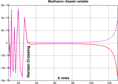
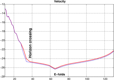
Figure 2: Left: Evolution of the Mukhanov-Sasaki variable. The non-trivial shape of the potential leads to evolution of the variable after horizon crossing. The late time amplification is due to the change in curvature of the potential after the inflection point; the negative mass squared of the inflaton leads to a tachyonic amplification of the modes. Right: The corresponding time derivative of the same Mukhanov-Sasaki variable. We plot the absolute value of the velocity on a log scale. The velocity increases after the inflaton passes the inflection point. To calculate the adiabatic and entropy spectra we take a snapshot just before inflation ends.

A snapshot of the perturbations is taken just before inflation ends and these are then decomposed into adiabatic and entropic components following Eqs. (55) and (57) to obtain the final super-horizon power spectra.

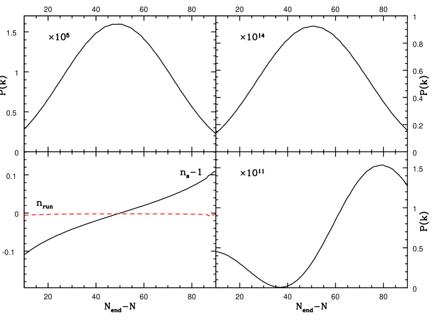
Figure 3: Upper Left: The adiabatic spectrum has the same shape for single or multi-brane models and is insensitive to the initial positions of the branes. Upper Right: The entropy spectrum for coincident branes or a single brane. Lower Right: The entropy spectrum for the same model, with the branes starting from different locations. The amplitude of the spectrum is still 6 orders of magnitude smaller than that of the adiabatic perturbations Lower Left: The spectral index and its running for the adiabatic perturbations. The spectrum is blue before the inflaton passes the inflection point, so to get a red spectrum as suggested by the WMAP data we need 60 $e$-folds of inflation after passing the inflection point.

The single-brane model give the same qualitative results as the multi-brane model in which all the brane are initially coincident, and then roll together. We choose the parameters such that the adiabatic perturbations are COBE normalized for both the single-brane and the multi-brane models. The amplitude of the entropy spectrum is smaller for the single-brane case, but the spectra have the same shape. The results are shown in Fig. 3 together with the spectral index $n_{s}$ and running $dn_{s}/d\ln k$ as a function of $e$-folds.

The spectrum of adiabatic perturbations is initially blue before the inflection point and then becomes red. The running of the spectral index is small throughout the trajectory.

The shape of the entropy spectrum is highly sensitive to the trajectory in field space, a small change in the initial positions of the mobile branes results in a completely different shape of the spectrum as compared with the case of coincident branes. However the amplitude of the entropy spectrum is 6 orders of magnitude (9 orders of magnitude for coincident branes) smaller than the amplitude of the adiabatic perturbations. Such a small contribution to an isocurvature component of the primordial perturbations would be unobservable be even the most sensitive future CMB experiments.

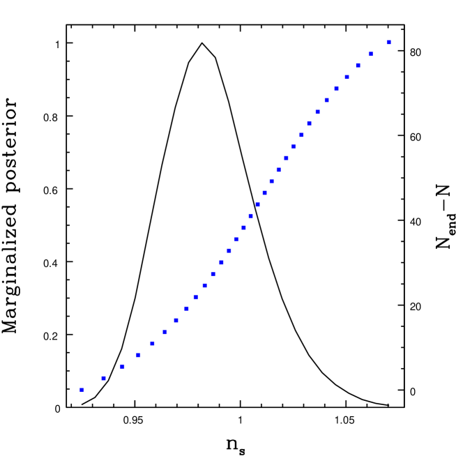
Figure 4: The marginalized posterior for the spectral index from the “WMAP5yr + CMB” Dunkley combination for the case where running of the spectral index is assumed to be zero. The square points are the value of the spectral tilt of the adiabatic perturbations shown in Fig. 3 which crossed the horizon at different times during inflation (shown on left axis). Only perturbations crossing the horizon at late times are compatible with the red spectra favoured by CMB data.

In Fig. 4 we compare the marginalized posterior distribution for the spectral index obtained from the “WMAP5yr + CMB” chains (see Dunkley for details of the data combination) with the spectral index of the perturbations which crossed the horizon at different $e$-foldings from the end of inflation ($N_{\rm end}$). The chains were obtained for a pure power law model of adiabatic primordial perturbations. Only the modes which exited the horizon after the inflection point are compatible with the red spectrum preferred by the data.

The comparison for when running of the spectral, $n_{\rm run}=dn_{s}/d\ln k$ index around a pivot point is allowed is shown in Fig. 5 for the same data combination. The pivot is at $k=0.002$ Mpc^-1 scales probed by current CMB experiments and the marginalized confidence contours are shown for the $n_{s}$, $n_{\rm run}$ plane. The smallness of the running observed in the models is in slight disagreement with the data which prefers a negative running of the index at around the 2-$\sigma$ level. The shift in the preferred $n_{s}$ value to $n_{s}\approx 1.05$ is due to the scale dependence of the spectral tilt in the presence of non-zero curvature.

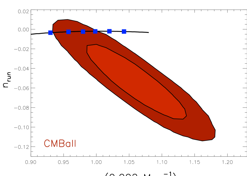
Figure 5: The adiabatic perturbations results of Fig. 3 plotted over the CMB constraints when both $n_{s}$ and $dn_{s}/d\ln k$ are fitted. The 68% and 95% confidence regions are obtained from the “WMAP5yr + CMB” Dunkley . The blue squares on the trajectory indicated, from left to right, the point at 20, 30, 40, 50, 60, and 70 $e$-foldings from the end of inflation. The smallness of the spectral running in the multi-brane models leads to some tension with the observations which prefer more negative running.

IX Conclusions

We analysed the possible signatures that brane-inflation models could give, that may be detectable in observations of the CMB spectrum. To do so we derived the evolution equation for the perturbations of the inflatons and metric and numerically evolved a large number of modes starting inside the horizon, all the way to the end of inflation. We then separated the fluctuations into adiabatic and entropy ones and derived their respective spectra. We found that the adiabatic spectrum is insensitive to the inflaton trajectories and has the has the same shape as was determined in earlier work Burgess:2004kv ; Cline:2005ty using the Sasaki-Stewart formalism Sasaki:1995aw . The entropy one is highly sensitive to the inflaton trajectories but its amplitude is too small to be observable. We also offered an analytical argument that in a large class of models where most of the $e$-folds come from a small region around an inflection point of the potential, the inflaton trajectory is almost a straight line and therefore the entropy perturbations are expected to be small. Thus multi-brane models solve a number of fine-tuning problems but due to their $e$-foldings coming from a reduced section of the field trajectory they display less phenomenology than single field models. This argument would lead us to expect that other potentially observable effects such as non-Gaussianities would also have a low amplitude in these models. Typically large values of the non-Gaussian $f_{\rm NL}$ parameter are produced during periods of high acceleration in the field trajectory which are not present in these models ng .

Interestingly, the old models of brane inflation using branes oriented at angles and toroidal compactifications Jones:2002cv ; Burgess:2001fx ; GarciaBellido:2001ky ; Shandera:2003gx have highly non-trivial inflaton trajectories as a result of the brane interaction inside a compact manifold. This leaves open the possibility that more complicated models, like multi-throat models Iizuka:2004ct will feature non-trivial inflaton trajectories and therefore observable features in the power spectrum and non-Gaussianity.

As we have shown the models have no particular problem in reproducing the observed tilt in the power spectrum but as expected in models that probe short trajectories, the running is small. If the observed running is confirmed to be at the current best-fit value of $dn_{s}/d\ln k\approx-0.05$ with increasing significance in future measurements it may turn out to be the strongest constraint on these models. As with most multi-field inflation models a detection of a gravitational wave background would also be in conflict with the models since the tensor perturbation are not boosted by the number of fields contributing to inflating the universe.

X Acknowledgements

The research of H.S. was supported in part by the EU under MRTN contract MRTN-CT-2004-005104 and by PPARC under rolling grant PP/D0744X/1. H.S. would also like to thank Oisin Mac Conamhna for discussions.

Appendix A Details of the calculation

A.1 The F-term potential

The F-term is calculated with the usual formula:

$$V_{F}=e^{\mathcal{K}}\left(K^{\overline{a}b}\overline{D_{a}W}D_{b}W-3\left|W\right|^{2}\right),$$ (62)

where

$${\mathcal{K}}=-3\log\left(r\right).$$ (63)

The covariant derivatives are expressed as:

$$D_{T}W = \partial_{T}W+W\partial_{T}{\mathcal{K}}=\partial_{T}W-\frac{3}{r}W$$ (64)

$$D_{\phi_{i}}W = \partial_{\phi_{i}}W+W\partial_{\phi_{i}}{\mathcal{K}}=\frac{\partial f_{i}}{\partial\phi_{i}}\frac{3}{r}W$$ (65)

$$\overline{D_{T}W} = \partial_{\overline{T}}\overline{W}+\overline{W}\partial_{\overline{T}}{\mathcal{K}}=\partial_{\overline{T}}\overline{W}-\frac{3}{r}\overline{W}$$ (66)

$$\overline{D_{\phi_{i}}W} = \partial_{\overline{\phi_{i}}}\overline{W}+\overline{W}\partial_{\overline{\phi_{i}}}{\mathcal{K}}=\frac{\partial f_{i}}{\partial\phi_{i}^{*}}\frac{3}{r}\overline{W}$$ (67)

The inverse Kähler metric needed in the expression above, can be calculated analytically in the general case:

$${\mathcal{K}}^{\overline{a}b}=\frac{r}{3}\left(\begin{array}[]{ccccc}r+\frac{\partial f_{1}}{\partial\varphi_{1}}\frac{\partial f_{1}}{\partial\varphi_{1}^{*}}/\frac{\partial^{2}f_{1}}{\partial\varphi_{1}\partial\varphi_{1}^{*}}+\dots+\frac{\partial f_{n}}{\partial\varphi_{n}}\frac{\partial f_{n}}{\partial\varphi_{n}^{*}}/\frac{\partial^{2}f_{n}}{\partial\varphi_{n}\partial\varphi_{n}^{*}}&\frac{\partial f_{1}}{\partial\varphi_{1}^{*}}/\frac{\partial^{2}f_{1}}{\partial\varphi_{1}\partial\varphi_{1}^{*}}&\frac{\partial f_{2}}{\partial\varphi_{2}^{*}}/\frac{\partial^{2}f_{2}}{\partial\varphi_{2}\partial\varphi_{2}^{*}}&\ldots&\frac{\partial f_{n}}{\partial\varphi_{n}^{*}}/\frac{\partial^{2}f_{n}}{\partial\varphi_{n}\partial\varphi_{n}^{*}}\\ \frac{\partial f_{1}}{\partial\varphi_{1}}/\frac{\partial^{2}f_{1}}{\partial\varphi_{1}\partial\varphi_{1}^{*}}&1/\frac{\partial^{2}f_{1}}{\partial\varphi_{1}\partial\varphi_{1}^{*}}&0&\ldots&0\\ \frac{\partial f_{2}}{\partial\varphi_{2}}/\frac{\partial^{2}f_{2}}{\partial\varphi_{2}\partial\varphi_{2}^{*}}&0&1/\frac{\partial^{2}f_{2}}{\partial\varphi_{2}\partial\varphi_{2}^{*}}&\ldots&0\\ \vdots&\vdots&\vdots&\ddots&\vdots\\ \frac{\partial f_{n}}{\partial\varphi_{n}}/\frac{\partial^{2}f_{n}}{\partial\varphi_{n}\partial\varphi_{n}^{*}}&0&0&\ldots&1/\frac{\partial^{2}f_{n}}{\partial\varphi_{n}\partial\varphi_{n}^{*}}\end{array}\right)$$

Using the above expression for the inverse Kähler metric one obtains the following terms:

$$K^{\overline{T}T}\overline{D_{T}W}D_{T}W = \frac{r}{3}\left(\partial_{\overline{T}}\overline{W}-\frac{3}{r}\overline{W}\right)\left(\partial_{T}W-\frac{3}{r}W\right)\left(r+\frac{\frac{\partial f_{1}}{\partial\phi_{1}}\frac{\partial f_{1}}{\partial\phi_{1}^{*}}}{\frac{\partial^{2}f_{1}}{\partial\phi_{1}\partial\phi_{1}^{*}}}+\dots+\frac{\frac{\partial f_{n}}{\partial\phi_{n}}\frac{\partial f_{n}}{\partial\phi_{n}^{*}}}{\frac{\partial^{2}f_{n}}{\partial\phi_{n}\partial\phi_{n}^{*}}}\right)$$ (68)

$$K^{\overline{T}\phi_{i}}\overline{D_{T}W}D_{\phi_{i}}W = \frac{r}{3}\left(\partial_{\overline{T}}\overline{W}-\frac{3}{r}\overline{W}\right)W\left(\frac{3}{r}\frac{\partial f_{1}}{\partial\phi_{1}}\frac{\frac{\partial f_{1}}{\partial\phi_{1}^{*}}}{\frac{\partial^{2}f_{1}}{\partial\phi_{1}\partial\phi_{1}^{*}}}+\dots+\frac{3}{r}\frac{\partial f_{n}}{\partial\phi_{n}}\frac{\frac{\partial f_{n}}{\partial\phi_{n}^{*}}}{\frac{\partial^{2}f_{n}}{\partial\phi_{n}\partial\phi_{n}^{*}}}\right)$$ (69)

$$K^{\overline{\phi_{i}}T}\overline{D_{\phi_{i}}W}D_{T}W = \frac{r}{3}\left(\partial_{T}W-\frac{3}{r}W\right)\overline{W}\left(\frac{3}{r}\frac{\partial f_{1}}{\partial\phi_{1}^{*}}\frac{\frac{\partial f_{1}}{\partial\phi_{1}}}{\frac{\partial^{2}f_{1}}{\partial\phi_{1}\partial\phi_{1}^{*}}}+\dots+\frac{3}{r}\frac{\partial f_{n}}{\partial\phi_{n}^{*}}\frac{\frac{\partial f_{n}}{\partial\phi_{n}}}{\frac{\partial^{2}f_{n}}{\partial\phi_{n}\partial\phi_{n}^{*}}}\right)$$ (70)

$$K^{\overline{\phi_{i}}\phi_{j}}\overline{D_{\phi_{i}}W}D_{\phi_{j}}W = \frac{r}{3}W\overline{W}\left(\frac{9}{r^{2}}\frac{\partial f_{1}}{\partial\phi_{1}}\frac{\partial f_{1}}{\partial\phi_{1}^{*}}\frac{1}{\frac{\partial^{2}f_{1}}{\partial\phi_{1}\partial\phi_{1}^{*}}}+\dots+\frac{9}{r^{2}}\frac{\partial f_{n}}{\partial\phi_{n}}\frac{\partial f_{n}}{\partial\phi_{n}^{*}}\frac{1}{\frac{\partial^{2}f_{n}}{\partial\phi_{n}\partial\phi_{n}^{*}}}\right)$$ (71)

Adding all the above terms and $-3\left|W\right|^{2}$ we obtain the F-term:

$$V_{F}=\frac{1}{r^{3}}\left[\frac{r^{2}}{3}\partial_{\overline{T}}\overline{W}\partial_{T}W\left(1+\frac{\frac{\partial f_{1}}{\partial\phi_{1}}\frac{\partial f_{1}}{\partial\phi_{1}^{*}}}{r\frac{\partial^{2}f_{1}}{\partial\phi_{1}\partial\phi_{1}^{*}}}+\dots+\frac{\frac{\partial f_{n}}{\partial\phi_{n}}\frac{\partial f_{n}}{\partial\phi_{n}^{*}}}{r\frac{\partial^{2}f_{n}}{\partial\phi_{n}\partial\phi_{n}^{*}}}\right)-r\left(W\partial_{\overline{T}}\overline{W}+\overline{W}\partial_{T}W\right)\right].$$ (72)

We assumed that the superpotential itself is independent of the fields $\phi_{1}\dots\phi_{n}$.

For a racetrack superpotential (9) the corresponding F-term potential becomes:

$$V_{F}=\frac{e^{-a\sigma}}{3r^{2}\frac{\partial^{2}f}{\partial\phi\partial\overline{\phi}}\frac{\partial^{2}g}{\partial\psi\partial\overline{\psi}}}\left[aA^{2}e^{-a\sigma}\left(a\frac{\partial^{2}g}{\partial\psi\partial\overline{\psi}}\frac{\partial f}{\partial\phi}\frac{\partial f}{\partial\overline{\phi}}+a\frac{\partial^{2}f}{\partial\phi\partial\overline{\phi}}\frac{\partial g}{\partial\psi}\frac{\partial g}{\partial\overline{\psi}}+\frac{\partial^{2}f}{\partial\phi\partial\overline{\phi}}\frac{\partial^{2}g}{\partial\psi\partial\overline{\psi}}\left(6+ar\right)\right)+\right.$$

$$\left.3aAw_{0}\frac{\partial^{2}f}{\partial\phi\partial\overline{\phi}}\frac{\partial^{2}g}{\partial\psi\partial\overline{\psi}}\cos\left(a\omega\right)\right]+$$

$$\frac{e^{-b\sigma}}{3r^{2}\frac{\partial^{2}f}{\partial\phi\partial\overline{\phi}}\frac{\partial^{2}g}{\partial\psi\partial\overline{\psi}}}\left[bB^{2}e^{-b\sigma}\left(b\frac{\partial^{2}g}{\partial\psi\partial\overline{\psi}}\frac{\partial f}{\partial\phi}\frac{\partial f}{\partial\overline{\phi}}+b\frac{\partial^{2}f}{\partial\phi\partial\overline{\phi}}\frac{\partial g}{\partial\psi}\frac{\partial g}{\partial\overline{\psi}}+\frac{\partial^{2}f}{\partial\phi\partial\overline{\phi}}\frac{\partial^{2}g}{\partial\psi\partial\overline{\psi}}\left(6+br\right)\right)+\right.$$

$$\left.3bBw_{0}\frac{\partial^{2}f}{\partial\phi\partial\overline{\phi}}\frac{\partial^{2}g}{\partial\psi\partial\overline{\psi}}\cos\left(b\omega\right)\right]+\frac{e^{-\left(a+b\right)\sigma}}{3r^{2}\frac{\partial^{2}f}{\partial\phi\partial\overline{\phi}}\frac{\partial^{2}g}{\partial\psi\partial\overline{\psi}}}\left[3AB\left(a+b\right)\frac{\partial^{2}f}{\partial\phi\partial\overline{\phi}}\frac{\partial^{2}g}{\partial\psi\partial\overline{\psi}}+\right.$$

$$\left.abAB\left(\frac{\partial^{2}g}{\partial\psi\partial\overline{\psi}}\frac{\partial f}{\partial\phi}\frac{\partial f}{\partial\overline{\phi}}+\frac{\partial^{2}f}{\partial\phi\partial\overline{\phi}}\frac{\partial g}{\partial\psi}\frac{\partial g}{\partial\overline{\psi}}-r\frac{\partial^{2}f}{\partial\phi\partial\overline{\phi}}\frac{\partial^{2}g}{\partial\psi\partial\overline{\psi}}\right)\right]\cos\left(\left(a-b\right)\omega\right)$$ (73)

The expression above becomes much simpler if the functions $f$ and $g$ are taken to be the simplest ones, $f=\phi\overline{\phi}$ and $g=\psi\overline{\psi}$.

A.2 Perturbation of the kinetic term

This is the first term in Eq. (25):

$$\frac{1}{\sqrt{-g}}\partial_{\mu}\left[\sqrt{-g}g^{\mu\nu}\partial_{\nu}\phi^{K}\right],$$ (74)

and we expand this term as follows:

$$\frac{1}{\sqrt{-\det\left(g+\delta g\right)}}\partial_{\mu}\left[\sqrt{-\det\left(g+\delta g\right)}\left(g^{\mu\nu}+\delta g^{\mu\nu}\right)\partial_{\nu}\left(\phi^{K}+\delta\phi^{K}\right)\right]=$$

$$\underbrace{\frac{1}{\sqrt{-g}}\partial_{\mu}\left[\sqrt{-g}g^{\mu\nu}\partial_{\nu}\phi^{K}\right]}_{\text{background}}+\frac{1}{\sqrt{-g}}\partial_{\mu}\left[\sqrt{-g}g^{\mu\nu}\partial_{\nu}\delta\phi^{K}\right]+\frac{1}{\sqrt{-g}}\partial_{\mu}\left[\sqrt{-g}\delta g^{\mu\nu}\partial_{\nu}\phi^{K}\right]$$

$$+\frac{1}{\sqrt{-g}}\partial_{\mu}\left[\sqrt{-g}\frac{1}{2}Tr\left[g^{-1}\delta g\right]g^{\mu\nu}\partial_{\nu}\phi^{K}\right]-\frac{1}{\sqrt{-g}}\frac{1}{2}Tr\left[g^{-1}\delta g\right]\partial_{\mu}\left[\sqrt{-g}g^{\mu\nu}\partial_{\nu}\phi^{K}\right]$$ (75)

In the above equation we used the expansion of a determinant:

$$\det\left[{g+\delta g}\right]=\det\left[g\left({\mathbbm{1}}+g^{-1}\delta g\right)\right]=\det g\det\left[\left({\mathbbm{1}}+g^{-1}\delta g\right)\right]=\det ge^{Tr\log\left({\mathbbm{1}}+g^{-1}\delta g\right)}\simeq$$

$$\det ge^{Tr\left[g^{-1}\delta g\right]}\simeq\det g\left({\mathbbm{1}}+Tr\left[g^{-1}\delta g\right]\right)$$ (76)

and therefore:

$$\sqrt{-\det\left[{g+\delta g}\right]}=\sqrt{-\det g}\left(1+\frac{1}{2}Tr\left[g^{-1}\delta g\right]\right).$$ (77)

We now proceed to simplify each one of the 4 terms in Eq.(75) above using the background metric Eq.(22) and the fact that the background fields and metric depend only on time. We write the Laplacian of a generic field $\Phi$ in terms of the momentum as $\partial^{m}\partial_{m}\Phi=-k^{2}\Phi$ and proceed with the details of the perturbations of each of the 4 terms in Eq.(75):

A.2.1 1st term

This term is straightforward to compute, as it involves only the perturbation of the scalar field:

$$\frac{1}{\sqrt{-g}}\partial_{\mu}\left[\sqrt{-g}g^{\mu\nu}\partial_{\nu}\delta\phi^{K}\right]=\frac{1}{a^{3}}\partial_{\mu}\left[a^{3}g^{\mu\nu}\partial_{\nu}\delta\phi^{K}\right]=$$

$$-\frac{1}{a^{3}}\partial_{0}\left[a^{3}\dot{\delta\phi^{K}}\right]+\frac{1}{a^{2}}\partial_{m}\partial^{m}\delta\phi^{K}=-\ddot{\delta\phi^{K}}-3\frac{\dot{a}}{a}\dot{\delta\phi^{K}}-\frac{k^{2}}{a^{2}}\delta\phi^{K}$$ (78)

A.2.2 2nd term

In order to proceed we will need the form of the perturbations of the inverse metric. We can easily find the inverse metric imposing the condition that

$$\left(g_{\mu\nu}+\delta g_{\mu\nu}\right)\left(g^{\nu\lambda}+\delta g^{\nu\lambda}\right)=\delta_{\mu}^{\lambda},$$ (79)

to first order in the perturbations. We find the inverse metric to have the expression:

$$g^{\mu\nu}+\delta g^{\mu\nu}=\left(\begin{array}[]{cc}-\left(1-2A\left(t,{\bf x}\right)\right)&\frac{1}{a}\left(t\right)B_{,i}\left(t,{\bf x}\right)\\ \frac{1}{a}\left(t\right)B_{,i}\left(t,{\bf x}\right)&\frac{1}{a^{2}}\left(t\right)\left[\left(1+2\psi\left(t,{\bf x}\right)\right)\delta_{ij}-2E_{,ij}\left(t,{\bf x}\right)\right].\end{array}\right)$$ (80)

With this expression the 2nd kinetic term perturbation becomes:

$$\frac{1}{\sqrt{-g}}\partial_{\mu}\left[\sqrt{-g}\delta g^{\mu\nu}\partial_{\nu}\phi^{K}\right]=\frac{1}{a^{3}}\partial_{0}\left[a^{3}\delta g^{00}\dot{\phi^{K}}\right]+\frac{1}{a^{3}}\partial_{m}\left[a^{3}\delta g^{m0}\dot{\phi^{K}}\right]=$$

$$\frac{1}{a^{3}}\partial_{0}\left[a^{3}\left(2A\right)\dot{\phi^{K}}\right]+\partial_{m}\left[\frac{B_{,m}}{a}\dot{\phi^{K}}\right]=2A\ddot{\phi^{K}}+6A\frac{\dot{a}}{a}\dot{\phi^{K}}+\dot{2A}\dot{\phi^{K}}+\frac{1}{a}\dot{\phi^{K}}\partial^{m}\partial_{m}B$$ (81)

A.2.3 3rd term

This terms has the expression:

$$\frac{1}{\sqrt{-g}}\partial_{\mu}\left[\sqrt{-g}\frac{1}{2}Tr\left[g^{-1}\delta g\right]g^{\mu\nu}\partial_{\nu}\phi^{K}\right]=-\frac{1}{a^{3}}\partial_{0}\left[a^{3}\frac{1}{2}Tr\left[g^{-1}\delta g\right]\dot{\phi^{K}}\right]=$$

$$-\ddot{\phi^{K}}\frac{1}{2}Tr\left[g^{-1}\delta g\right]-\dot{\phi^{K}}\frac{1}{2}\dot{Tr\left[g^{-1}\delta g\right]}-\frac{3\dot{a}}{2a}\dot{\phi^{K}}Tr\left[g^{-1}\delta g\right]$$ (82)

where the trace of the metric perturbation has the form::

$$\frac{1}{2}Tr\left[g^{-1}\delta g\right]=A-3\psi+E_{,11}+E_{,22}+E_{,33}=A-3\psi-k^{2}E.$$ (83)

A.2.4 4th term

Finally, this is the simplest of the 4 terms and it has the expression:

$$-\frac{1}{\sqrt{-g}}\frac{1}{2}Tr\left[g^{-1}\delta g\right]\partial_{\mu}\left[\sqrt{-g}g^{\mu\nu}\partial_{\nu}\phi^{K}\right]=-\frac{1}{2a^{3}}Tr\left[g^{-1}\delta g\right]\partial_{0}\left[a^{3}\underbrace{\left(-1\right)}_{g^{00}}\dot{\phi^{K}}\right]=$$

$$\frac{1}{2}\ddot{\phi^{K}}Tr\left[g^{-1}\delta g\right]+\frac{3\dot{a}}{2a}\dot{\phi^{K}}Tr\left[g^{-1}\delta g\right]$$ (84)

We see that these two terms we obtained will cancel 2 of the terms from the previous expression. We can now move on to the potential terms.

A.3 Details of the Calculations: M-S variables

We present here the details of the calculation for the term:

$$-2A_{Q}G^{KI}\frac{\partial V}{\partial\phi^{I}}+\left[\dot{A_{Q}}+\frac{1}{H}\frac{k^{2}}{a^{2}}\Psi\right]\dot{\phi^{K}},$$ (85)

appearing on the R.H.S. of the perturbation equation. We want it to take the appropriate form in terms of the Sasaki-Mukhanov variables. We will therefore use Eq. (49) and (51) in the expression above as well as the equation of motion for the background fields, Eq. (23). The expression above becomes:

$$-2A_{Q}G^{KI}\frac{\partial V}{\partial\phi^{I}}+\left[\dot{A_{Q}}+\frac{1}{H}\frac{k^{2}}{a^{2}}\Psi\right]\dot{\phi^{K}}=-\frac{8\pi G}{H}\underbrace{G^{KI}\frac{\partial V}{\partial\phi^{I}}}_{\text{eq. mot.}}G_{LM}\dot{\phi}^{L}\delta\phi^{M}+$$

$$\frac{4\pi G}{H}\dot{\phi}^{K}\left[-\frac{\dot{H}}{H}G_{IJ}\dot{\phi}^{I}\delta\phi^{J}+\frac{\partial G_{IJ}}{\partial\phi^{L}}\dot{\phi^{I}}\dot{\phi}^{L}\delta{\phi^{J}}+G_{IJ}\ddot{\phi}^{I}\delta\phi^{J}+G_{IJ}\dot{\phi}^{I}\delta\dot{\phi}^{J}+\right.$$

$$\underbrace{\frac{4\pi G}{H}G_{LM}\dot{\phi}^{L}\dot{\phi}^{M}G_{IJ}\dot{\phi}^{I}\delta\phi^{J}}_{\text{calculate }\dot{H}/H}-G_{IJ}\dot{\phi}^{I}\delta\dot{\phi}^{J}-\frac{1}{2}\frac{\partial G_{IJ}}{\partial\phi^{L}}\dot{\phi}^{I}\dot{\phi}^{J}\delta\phi^{L}-\underbrace{\frac{\partial V}{\partial\phi^{L}}}_{\text{eq. mot.}}\delta\phi^{L}$$

$$\Biggl{.}-3HG_{IJ}\dot{\phi}^{I}\delta\phi^{J}\Biggr{]}$$ (86)

We use the equation of motion to express $\frac{\partial V}{\partial\phi^{L}}$ in terms of the fields and their derivatives. We also notice that the terms $G_{IJ}\dot{\phi}^{I}\delta\dot{\phi}^{J}$ cancel and the terms containing the derivatives of the Kähler metric can be combined to form the Christoffel symbol with all indices lowered.

$$\frac{\partial G_{IJ}}{\partial\phi^{L}}\dot{\phi^{I}}\dot{\phi}^{L}\delta{\phi^{J}}-\frac{1}{2}\frac{\partial G_{IJ}}{\partial\phi^{L}}\dot{\phi}^{I}\dot{\phi}^{J}\delta\phi^{L}=$$

$$\frac{1}{2}\left[\frac{\partial G_{LJ}}{\partial\phi^{I}}+\frac{\partial G_{IL}}{\partial\phi^{J}}-\frac{\partial G_{IJ}}{\partial\phi^{L}}\right]\dot{\phi}^{I}\dot{\phi}^{J}\delta\phi^{L}=\Gamma_{LIJ}\dot{\phi}^{I}\dot{\phi}^{J}\delta\phi^{L}$$ (87)

Finally, the term $\frac{4\pi G}{H}G_{LM}\dot{\phi}^{L}\dot{\phi}^{M}G_{IJ}\dot{\phi}^{I}\delta\phi^{J}$ can be related to $\dot{H}/H$. We start out by calculating $\dot{H}/H$:

$$\frac{\dot{H}}{H}=\frac{1}{2\left(\frac{1}{2}G_{IJ}\dot{\phi}^{I}\dot{\phi}^{J}+V\right)}\left[G_{IJ}\ddot{\phi}^{I}\dot{\phi}^{J}+\frac{\partial G_{IJ}}{\partial\phi^{L}}\dot{\phi}^{I}\dot{\phi}^{J}\dot{\phi}^{L}+\frac{\partial V}{\partial\phi^{L}}\dot{\phi}^{L}\right]$$

$$=\frac{1}{2\left(\frac{1}{2}G_{IJ}\dot{\phi}^{I}\dot{\phi}^{J}+V\right)}\left[-G_{IJ}\dot{\phi}^{J}\left(3H\dot{\phi}^{I}+G^{IL}\frac{\partial V}{\partial\phi^{L}}+\Gamma^{I}_{LM}\dot{\phi}^{L}\dot{\phi}^{M}\right)\right.$$

$$\left.+\frac{\partial G_{IJ}}{\partial\phi^{L}}\dot{\phi}^{I}\dot{\phi}^{J}\dot{\phi}^{L}+\frac{\partial V}{\partial\phi^{L}}\dot{\phi}^{L}\right]$$

$$=\frac{-3HG_{IJ}\dot{\phi}^{I}\dot{\phi}^{J}}{2\left(\frac{1}{2}G_{IJ}\dot{\phi}^{I}\dot{\phi}^{J}+V\right)}=-\frac{4\pi GHG_{IJ}\dot{\phi}^{I}\dot{\phi}^{J}}{H^{2}}=-\frac{4\pi G}{H}G_{IJ}\dot{\phi}^{I}\dot{\phi}^{J}$$ (88)

The above result tells us that we can substitute:

$$\frac{4\pi G}{H}G_{LM}\dot{\phi}^{L}\dot{\phi}^{M}G_{IJ}\dot{\phi}^{I}\delta\phi^{J}=-\frac{\dot{H}}{H}G_{IJ}\dot{\phi}^{I}\delta\phi^{J}.$$ (89)

The expression we want to calculate becomes:

$$-2A_{Q}G^{KI}\frac{\partial V}{\partial\phi^{I}}+\left[\dot{A_{Q}}+\frac{1}{H}\frac{k^{2}}{a^{2}}\Psi\right]\dot{\phi^{K}}=$$

$$\frac{8\pi G}{H}\left(\ddot{\phi}^{K}+3H\dot{\phi}^{K}+\Gamma^{K}_{IJ}\dot{\phi}^{I}\dot{\phi}^{J}\right)G_{LM}\dot{\phi}^{L}\delta\phi^{M}$$

$$+\frac{4\pi G}{H}\dot{\phi}^{K}\left[-2\frac{\dot{H}}{H}G_{IJ}\dot{\phi}^{I}\delta\phi^{J}+\Gamma_{LIJ}\dot{\phi}^{I}\dot{\phi}^{J}\delta\phi^{L}+G_{IJ}\ddot{\phi}^{I}\delta\phi^{J}+\right.$$

$$\left.\left(\ddot{\phi}^{M}+3H\dot{\phi}^{M}+\Gamma^{M}_{IJ}\dot{\phi}^{I}\dot{\phi}^{J}\right)G_{ML}\delta\phi^{L}-3HG_{IJ}\dot{\phi}^{I}\delta\phi^{J}\right]=$$

$$\frac{8\pi G}{H}\left[-\frac{\dot{H}}{H}G_{LM}\dot{\phi}^{L}\dot{\phi}^{M}\delta\phi^{J}+G_{LM}\dot{\phi}^{L}\ddot{\phi}^{K}\delta\phi^{M}+\right.$$

$$G_{LM}\ddot{\phi}^{L}\dot{\phi}^{K}\delta\phi^{M}+3HG_{LM}\dot{\phi}^{L}\dot{\phi}^{K}\delta\phi^{M}$$

$$\left.+\Gamma_{LIJ}\dot{\phi}^{I}\dot{\phi}^{J}\delta\phi^{L}\dot{\phi}^{K}+\Gamma^{K}_{IJ}\dot{\phi}^{I}\dot{\phi}^{J}G_{LM}\dot{\phi}^{L}\delta\phi^{M}\right]=$$

$$\frac{8\pi G}{a^{3}}\left[G_{IJ}\frac{\partial}{\partial t}\left(\frac{a^{3}\dot{\phi}^{I}\delta\phi^{K}}{H}\right)\right]\delta\phi^{J}+\frac{8\pi G}{H}\left[\Gamma_{LIJ}\dot{\phi}^{I}\dot{\phi}^{J}\delta\phi^{L}\dot{\phi}^{K}+\Gamma^{K}_{IJ}\dot{\phi}^{I}\dot{\phi}^{J}G_{LM}\dot{\phi}^{L}\delta\phi^{M}\right]$$ (90)

In the end we obtain the equation:

$$\ddot{Q^{K}}+3H\dot{Q^{K}}+\frac{k^{2}}{a^{2}}Q^{K}+2\Gamma_{IJ}^{K}\dot{\phi^{I}}\dot{Q^{J}}+\left[G^{KI}\frac{\partial^{2}V}{\partial\phi^{I}\partial\phi^{J}}+\frac{\partial G^{KI}}{\partial\phi^{J}}\frac{\partial V}{\partial\phi^{I}}\right.$$

$$+\frac{\partial\Gamma_{IJ}^{K}}{\partial\phi^{L}}\dot{\phi^{I}}\dot{\phi^{J}}\dot{\phi}^{L}-\left(\frac{8\pi G}{a^{3}}\right)G_{IJ}\frac{\partial}{\partial t}\left(\frac{a^{3}\dot{\phi}^{K}\dot{\phi}^{I}}{H}\right)$$

$$\left.-\left(\frac{8\pi G}{H}\right)\Gamma_{ILJ}\dot{\phi}^{K}\dot{\phi}^{I}\dot{\phi}^{L}-\left(\frac{8\pi G}{H}\right)\Gamma^{K}_{LM}\dot{\phi}^{L}\dot{\phi}^{M}G_{IJ}\dot{\phi}^{I}\right]Q^{J}=0$$ (91)

References

- (1) G. R. Dvali and S. H. H. Tye, Phys. Lett. B 450, 72 (1999) [arXiv:hep-ph/9812483].
- (2) C. P. Burgess, M. Majumdar, D. Nolte, F. Quevedo, G. Rajesh and R. J. Zhang, JHEP 0107, 047 (2001) [arXiv:hep-th/0105204].
- (3) J. Garcia-Bellido, R. Rabadan and F. Zamora, JHEP 0201, 036 (2002) [arXiv:hep-th/0112147].
- (4) N. T. Jones, H. Stoica and S. H. H. Tye, JHEP 0207, 051 (2002) [arXiv:hep-th/0203163].
- (5) J. J. Blanco-Pillado et al., JHEP 0411, 063 (2004) [arXiv:hep-th/0406230].
- (6) J. P. Conlon and F. Quevedo, JHEP 0601, 146 (2006) [arXiv:hep-th/0509012].
- (7) A. Shafieloo and T. Souradeep, Phys. Rev. D 70, 043523 (2004) [arXiv:astro-ph/0312174]. N. Kogo, M. Matsumiya, M. Sasaki and J. Yokoyama, Astrophys. J. 607, 32 (2004) [arXiv:astro-ph/0309662]. L. Verde and H. V. Peiris, arXiv:0802.1219 [astro-ph].
- (8) M. R. Nolta et al. [WMAP Collaboration], arXiv:0803.0593 [astro-ph].
- (9) J. Martin and C. Ringeval, Phys. Rev. D 69, 083515 (2004) [arXiv:astro-ph/0310382]. C. Pahud, M. Kamionkowski and A. R. Liddle, arXiv:0807.0322 [astro-ph]. L. Covi, J. Hamann, A. Melchiorri, A. Slosar and I. Sorbera, Phys. Rev. D 74, 083509 (2006) [arXiv:astro-ph/0606452].
- (10) J. M. Maldacena, JHEP 0305, 013 (2003) [arXiv:astro-ph/0210603]. P. Creminelli, JCAP 0310, 003 (2003) [arXiv:astro-ph/0306122].
- (11) J. M. Cline and H. Stoica, Phys. Rev. D 72, 126004 (2005) [arXiv:hep-th/0508029].
- (12) A. R. Liddle, A. Mazumdar and F. E. Schunck, Phys. Rev. D 58, 061301 (1998) [arXiv:astro-ph/9804177].
- (13) S. B. Giddings, S. Kachru and J. Polchinski, Phys. Rev. D 66, 106006 (2002) [arXiv:hep-th/0105097].
- (14) S. Kachru, R. Kallosh, A. Linde and S. P. Trivedi, Phys. Rev. D 68, 046005 (2003) [arXiv:hep-th/0301240].
- (15) V. F. Mukhanov, H. A. Feldman and R. H. Brandenberger, Phys. Rept. 215, 203 (1992).
- (16) M. Sasaki, Prog. Theor. Phys. 76, 1036 (1986).
- (17) D. Baumann, A. Dymarsky, I. R. Klebanov, L. McAllister and P. J. Steinhardt, Phys. Rev. Lett. 99, 141601 (2007) [arXiv:0705.3837 [hep-th]].
- (18) R. Kallosh and A. Linde, JHEP 0412, 004 (2004) [arXiv:hep-th/0411011].
- (19) D. Baumann, A. Dymarsky, I. R. Klebanov, J. M. Maldacena, L. P. McAllister and A. Murugan, JHEP 0611, 031 (2006) [arXiv:hep-th/0607050].
- (20) S. Kachru, R. Kallosh, A. Linde, J. M. Maldacena, L. P. McAllister and S. P. Trivedi, JCAP 0310, 013 (2003) [arXiv:hep-th/0308055].
- (21) C. P. Burgess, J. M. Cline, H. Stoica and F. Quevedo, JHEP 0409, 033 (2004) [arXiv:hep-th/0403119].
- (22) O. DeWolfe and S. B. Giddings, Phys. Rev. D 67, 066008 (2003) [arXiv:hep-th/0208123].
- (23) N. Iizuka and S. P. Trivedi, Phys. Rev. D 70, 043519 (2004) [arXiv:hep-th/0403203].
- (24) M. M. Caldarelli, Nucl. Phys. B 549, 499 (1999) [arXiv:hep-th/9809144].
- (25) C. Gordon, D. Wands, B. A. Bassett and R. Maartens, Phys. Rev. D 63, 023506 (2001) [arXiv:astro-ph/0009131]. B. J. W. van Tent and S. Groot Nibbelink, arXiv:hep-ph/0111370. Z. Lalak, D. Langlois, S. Pokorski and K. Turzynski, JCAP 0707, 014 (2007) [arXiv:0704.0212 [hep-th]].
- (26) W. Hu and M. J. White, Astrophys. J. 471, 30 (1996) [arXiv:astro-ph/9602019].
- (27) M. Sasaki and E. D. Stewart, Prog. Theor. Phys. 95, 71 (1996) [arXiv:astro-ph/9507001].
- (28) Dunkley, J., et al. 2008, ArXiv e-prints, 803, arXiv:0803.0586
- (29) S. Shandera, B. Shlaer, H. Stoica and S. H. H. Tye, JCAP 0402, 013 (2004) [arXiv:hep-th/0311207].