The mass content of the Sculptor dwarf spheroidal galaxy

Abstract

We present a new determination of the mass content of the Sculptor dwarf spheroidal galaxy, based on a novel approach which takes into account the two distinct stellar populations present in this galaxy. This method helps to partially break the well-known mass-anisotropy degeneracy present in the modelling of pressure-supported stellar systems.

1 Introduction

The determination of the mass content of galaxies is a fundamental step for our understanding of their formation and evolution. This is particularly true for small systems such as dwarf spheroidal galaxies (dSphs), whose total mass can determine their destiny as being fragile objects, strongly perturbed by supernovae explosions and/or interactions with the environment, or mostly undisturbed objects.

Part of the interest in determining the masses of dSphs has surely been driven by the fact that these galaxies, with mass-to-light (M/L) ratios up to 100s, appear to be the most dark matter (DM) dominated objects known to-date. This makes them potentially good testing grounds for different DM theories of galaxy formation; however at the moment it is still unclear if dSphs inhabit cusped DM profiles, as predicted by cold DM theories of galaxy formation, or cored profiles, typical of warmer kinds of DM. This distinction is often hampered by the degeneracies which are intrinsic to the method generally used to determine the mass of pressure-supported stellar systems, i.e. a Jeans analysis of the line-of-sight (l.o.s.) velocity dispersion obtained considering all stars as a single component embedded in an extended DM halo. This analysis is subject to the well known degeneracy between the mass distribution and the orbital motions of the individual stars in the system (mass-anisotropy degeneracy). Recent observations have shown that some dSphs host multiple stellar populations which have distinct spatial distribution, metallicity and kinematics. The presence of multiple stellar populations requires a modification in the way these systems are dynamically modelled to derive their mass content.

Here we describe the results of our determination of the mass content of the Sculptor (Scl) dSph by adopting a more detailed kinematic modelling than the traditional one, i.e. by considering Scl as two-(stellar) components embedded in an extended DM halo. We first briefly describe and discuss the observational properties of Scl derived from our work ([Tolstoy et al.(2004), Tolstoy et al. 2004]; [Battaglia (2007), Battaglia 2007]; [Battaglia et al. (2008), Battaglia et al. 2008]). We then move to the results of the two-component modelling; we show a clear example of the mass-anisotropy present when modelling Scl as a one-stellar component system, and finally discuss our results. For a more detailed description we refer to [Battaglia (2007), Battaglia (2007)] and [Battaglia et al. (2008), Battaglia et al. (2008)].

2 Observed properties of the Sculptor dSph

We acquired extended photometry from the ESO/2.2m WFI and VLT/FLAMES spectra (R$\sim$6500) in the Ca II  triplet region for hundreds of individual red giant branch (RGB) stars in Scl, out to its nominal tidal radius ([Tolstoy et al.(2004), Tolstoy et al. 2004]: 308 probable members; [Battaglia et al. (2008), Battaglia et al. 2008]: 470 probable members). We used these data to study the large scale kinematics and metallicity properties of Scl, and the spatial distribution of its stellar populations.

The combined information from the accurate line-of-sight velocities ($\pm$2 km s^-1 ) and metallicities ($\pm$0.15 dex) of RGB stars allowed us to unveil the presence of two distinct stellar populations with different spatial distribution, metallicity and kinematics: the metal rich (MR) stars ([Fe/H]$>-1.5$) are more centrally concentrated and show colder kinematics than the metal poor (MP) stars ([Fe/H]$<-1.7$), as can be seen from the line-of-sight (l.o.s.) velocity dispersion profiles in Fig. 1. The MR and MP RGB stars appear to trace, respectively, the red and blue horizontal branch (RHB, BHB) stars. The surface number density profile of RGB stars, representative of the overall stellar population of Scl, is well approximated by a two-component fit, where each component is given by the rescaled best-fitting profile derived from our photometry for the RHB and BHB stars. In contrast, a single profile (be it a Plummer, Sersic or King) does not appear to be a good approximation for the surface number density of RGB stars. Multiple stellar populations are known to exist also in other dSphs, such as Fornax ([Battaglia et al.(2006), Battaglia et al. 2006]) and Canes Venatici ([Ibata et al.(2006), Ibata et al. 2006]), and might be a common feature to this class of objects.

The large spatial coverage and statistics of this spectroscopic data-set has allowed the discovery of another interesting feature, i.e. a velocity gradient of 7.6 km s^-1 deg^-1 in the Galactic standard of rest (GSR) along the projected major axis of Scl. This gradient is likely to due intrinsic rotation, and not to tidal disruption (see [Battaglia (2007), Battaglia 2007] and [Battaglia et al. (2008), Battaglia et al. 2008] for discussion on this point), and this is the first time that statistically significant rotation is found in a dSph.

Among the other Milky Way (MW) dSphs, a significant velocity gradient is detected in Carina ([Muñoz et al.(2006), Muñoz et al. 2006]) and a mild one in Leo I ([Mateo et al. (2008), Mateo et al. 2008]), but these are interpreted as the result of tidal interaction with the MW. However, velocity gradients are not exclusive of the dSphs satellites of larger galaxies, but are present also in some of the isolated Local Group dSphs, such as Cetus ([Lewis et al.(2007), Lewis et al. 2007]) and Tucana (Fraternali et al., in preparation), which are unlikely to have ever interacted with either the MW or M31 and therefore suffered tidal disturbance. This might point to rotation as an intrinsic property of this class of objects and provide insights into the mechanisms that shaped their evolution. This might for instance favour scenarios in which the progenitors of dSphs were rotating systems which were transformed into prevalently pressure supported object by tidal stirring from their host galaxy (e.g., [Mayer et al.(2001), Mayer et al. 2001]). It would therefore be interesting to compare the frequency of occurrence of rotation among dSphs and other generally more isolated systems such as dwarf irregular galaxies and transition types. It is possible that more velocity gradients will be discovered in MW dSphs now that larger and more spatially extended velocity surveys are becoming available.

In the analysis presented here we always use rotation-subtracted GSR velocities.

3 The Jeans analysis

DSphs generally have low ellipticities and are presumably prevalently pressure supported, and therefore are commonly considered as spherical and with no streaming motions. Then, if the system is in dynamical equilibrium, the l.o.s. velocity dispersion predicted by the Jeans equation is (from [Binney & Mamon (1982), Binney & Mamon 1982])

$$\sigma_{\rm los}^{2}(R)=\frac{2}{\Sigma_{*}(R)}\int_{R}^{\infty}\frac{\rho_{*}(r)\sigma_{r,*}^{2}\ r}{\sqrt{r^{2}-R^{2}}}(1-\beta\frac{R^{2}}{r^{2}})dr$$ (1)

where $R$ is the projected radius (on the sky) and $r$ is the 3D radius. The l.o.s. velocity dispersion depends on: the mass surface density $\Sigma_{*}(R)$ and mass density $\rho_{*}(r)$ of the tracer, which in our case are the MR and the MP RGB stars; the tracer velocity anisotropy $\beta$, defined as $\beta=1-\ \sigma_{\theta}^{2}/\sigma_{r}^{2}$, and its radial velocity dispersion $\sigma_{r,*}$, which depends on the total mass distribution (for dSphs the contribution due to stellar mass is negligible). A unique solution for the mass profile can be determined from this equation if both the mass distribution of the tracer and $\beta(r)$ are known, although this solution is not guaranteed to produce a phase-space distribution function that is positive everywhere. However, proper motions for individual stars in the system would be necessary to derive $\beta(r)$ and this is not feasible yet. This causes the well-known mass-anisotropy degeneracy, which prevents a distinction amongst different DM profiles. Examples of this are present in the literature: the observed l.o.s. dispersion profiles of dSphs are both compatible with cored DM models, assuming that $\beta=0$ (e.g., [Gilmore et al.(2007), Gilmore et al. 2007]), and with cusped profiles, allowing for mildly tangential, constant with radius, $\beta$ (e.g. [Walker et al.(2007), Walker et al. 2007]). It is therefore advisable to explore several hypotheses for the behaviour of $\beta(r)$ and for the mass distribution when carrying out a Jeans analysis (see below).

In the following we explore the possibility that DM follows a cored (pseudo-isothermal sphere) or a cuspy distribution (NFW profile); we also explore two hypotheses for the behaviour of $\beta(r)$: constant with radius, and following an Osipkov-Merritt (OM) model (isotropic in the central parts and radial in the outskirts). The spatial distributions of the tracers are derived from our photometric data.

Figure 1: L.o.s. velocity dispersion profile (squares with errorbars), from rotation-subtracted GSR velocities, for the MR (left) and MP (right) RGB stars in Scl. The lines show the best-fitting pseudo-isothermal sphere (solid) and NFW model (dashed) in the hypothesis of $\beta=const$ (a,b) and $\beta=\beta_{\rm OM}$ (c,d). The models have reduced $\chi^{2}\sim 1.6$ (a,b), 0.6 (c) and 1 (d).

Two-components modelling Here we show the results of modelling Scl as a two-(stellar) component system embedded in a DM halo. Eq. 1 is applied separately to the MR and MP stars, assuming that they move in the same DM potential. We explore a range of core radii $r_{c}$ for the pseudo-isothermal sphere ($r_{c}\!=\!0.001,0.05,0.1,0.5,1$ kpc) and of concentrations $c$ for the NFW profile ($c\!=\!20,25,30,35$). By fixing these, each mass model has two free parameters left: the anisotropy and the DM halo mass (enclosed within the last measured point for the isothermal sphere, at 1.3 deg $=$ 1.8 kpc assuming a distance to Scl of 79 kpc, see [Mateo (1998), Mateo 1998]; and the virial mass in the case of the NFW model). We compute a $\chi^{2}$ for the MR and MP components separately ($\chi_{\rm MR}^{2}$ and $\chi_{\rm MP}^{2}$, respectively) by comparing the various models to the data. The best-fit is obtained by minimising the sum $\chi^{2}=\chi_{\rm MR}^{2}+\chi_{\rm MP}^{2}$.

Figure 1a,b shows the models with constant anisotropy, which can be excluded as in this case neither a cored or a cusped model is a good representation of the data ($\chi_{\rm min}^{2}\sim 17$). The situation is different in the hypothesis of an OM velocity anisotropy as shown in Fig. 1c,d). We find that a pseudo-isothermal sphere with a relatively large core ($r_{c}=$0.5 kpc, $M(<1.8\mathop{\rm kpc})=3.4\pm 0.7\times 10^{8}$  M_⊙) gives an excellent description of the data ($\chi_{\rm min}^{2}=6.9$). Also an NFW model is statistically consistent with the data ($c=20$, virial mass $M_{v}=2.2_{-0.7}^{+1.0}\times 10^{9}$  M_⊙, $\chi_{\rm min}^{2}=10.8$), but tends to over-predict the central values of the MR velocity dispersion. The mass within the last measured point ($\sim 2.4_{-0.7}^{+1.1}\times 10^{8}$  M_⊙) is consistent with the mass predicted by the best-fitting isothermal sphere model.

One-component modelling Figure 2 shows a clear example of the mass-anisotropy degeneracy when modelling Scl with the traditional one-component analysis. Just by changing the assumption on $\beta$ ($=$const. or $=\beta_{\rm OM}$), cored profiles with very different core radii and $M(<1.8\mathop{\rm kpc})$ give excellent fit to the data. An excellent fit is also an NFW profile, in the hypothesis of $\beta=$ const. These models are practically indistinguishable and all good ($\chi^{2}\sim 8$, reduced $\chi^{2}\sim 1.1$). No DM model can be favoured nor hypotheses on $\beta$.

Figure 2: a) Observed l.o.s. velocity dispersion profile, from rotation-subtracted GSR velocities, for all RGB stars in Scl (squares with error-bars), with overlaid the best-fits for a cored DM distribution (solid line: $\beta=\beta_{\rm OM}$ and $r_{c}=$0.5 kpc; dotted line: $\beta=$ const.and $r_{c}=$0.05 kpc), and an NFW DM distribution (dashed line: $\beta=$ const. and $c=35$). Panel b) and c) show the velocity anisotropy and mass distribution corresponding to the models in panel a). Note that the model with $r_{c}=$0.05 kpc is almost equivalent to a cusp.

4 Discussion and conclusions

The combined information of velocity and metallicity from a large sample of FLAMES spectra of individual stars in Scl has allowed us to separate the different kinematics of the two stellar populations in Scl, and to carry out a more detailed kinematic modelling which allows us to partially break the mass-anisotropy degeneracy.

Under the hypotheses explored for the behaviour of the velocity anisotropy $\beta(r)$, the two-component modelling indicates that a cored profile is slightly favoured over a cusped profile, as the latter tends to over-predict the central values (at $R\lesssim$ 0.1 kpc) of the MR velocity dispersion. It could be argued that the relatively large central dispersion predicted for the MR stars from the cusped profile could be lowered by allowing the velocity anisotropy of the MR population to be tangential at $R\lesssim$ 0.1 kpc. However it should be noted that in order to reproduce the rapid decline of the MR velocity dispersion profile, the MR $\beta(r)$ needs to become very radial already on the scale of 0.3-0.4 kpc, given the observed spatial distribution of MR stars. Observational determinations of $\beta$, either from direct measurement or from distribution functions, would be the most desirable (and definitive) solution to this issue.

[Strigari et al.(2007), Strigari et al. (2007)] showed that, independently of $\beta(r)$ and the total mass distribution of dSphs, the mass enclosed within 0.6 kpc (M_0.6) can be derived more accurately than at any other distance from the centre. However, given that the evolution of dSphs is most likely to be governed by their total mass and that dynamical analyses provide only the mass enclosed within the last measured point, it is important to have reliable determinations of the mass enclosed as farther out as possible. Our analysis shows that, independently of the adopted mass profile, the best fits from our two-component modelling yield consistent values for the mass enclosed within the last measured point, at 1.8kpc.

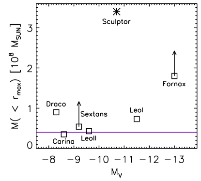
Figure 3: Left: Mass within the last measured point ($r_{\rm max}$) versus absolute $V$ magnitude, M_V, for MW dSphs. The masses are from [Walker et al.(2007), Walker et al. 2007] (squares), except for Scl which is from our two-components modelling (asterisk); M_V is from [Irwin and Hatzidimitriou (1995), Irwin & Hatzidimitriou (1995)]. The arrows indicate that the masses measured for Sextans and Fornax are likely to increase given that these objects have been surveyed just to 0.3 and 0.6 tidal radii. The solid line indicates a mass of 4$\times 10^{7}$  M_⊙. Right: Mass enclosed within $r$ for NFW halos of virial masses 2,4,8,20,40$\times 10^{8}$  M_⊙(solid lines), i.e. the range found by [Walker et al.(2007), Walker et al. (2007)] to fit the observed l.o.s. velocity dispersion profile of their sample of 7 dSphs. Concentrations are derived using the formula in [Koch et al. (2007), Koch et al. (2007)], extrapolated from [Jing & Suto (2000), Jing & Suto (2000)]. The dashed lines enclose masses between 2-7$\times 10^{7}$  M_⊙; the dotted line is placed at a radius of 0.6 kpc.

Finally we would like to comment on the issue that dwarf galaxies might be embedded in haloes of similar mass ($\sim 4\times 10^{7}$  M_⊙) as has been claimed in the literature. Figure 3(left) shows a revisited version of the mass enclosed within the last measured point versus absolute magnitude plot. The masses plotted are the ones derived in [Walker et al.(2007), Walker et al. (2007)] for a sample of dSphs, because they are derived from the most extended velocity samples and from a homogeneous analysis. For Scl we use our own determination, which is the most accurate so far. The figure shows that the DM mass of Scl is now much larger than the typical DM mass derived so far for the other dSphs. Also Fornax deviates considerably from the relation. In the plot shown here, the masses of Fornax and Sextans were derived from data extending out to $\sim$0.6 and 0.3 tidal radii, respectively. Given that Fornax and Sextans have been recently mapped much farther out (Fornax out to $\sim$ 1 tidal radius: Battaglia et al. 2006; Sextans out to $\sim$ 0.8 tidal radius: Battaglia et al. in preparation), their revised masses are likely to increase quite significantly, and introduce even larger dispersion in this plot. In some cases, M_0.6 has been used in this kind of analysis, instead than the mass enclosed within the last measured point. However, Fig. 3(right) shows that M_0.6 is very insensitive to the total mass of the dSph. In fact, NFW haloes of virial masses between 2-40 $\times 10^{8}$  M_⊙(i.e. in the range found by [Walker et al.(2007), Walker et al. 2007] to fit their samples of dSphs) give remarkably similar values of M_0.6, probably because at such a small distance there is not much sensitivity to the total mass. Therefore there is no indication of a common mass scale amongst the dSphs in the Local Group, while perhaps one may draw the conclusion of the existence of a minimum mass for the formation of dSphs.

References

- [Battaglia et al.(2006)] Battaglia, G., et al. 2006, A&A, 459, 423
- [Battaglia (2007)] Battaglia, G. 2007, PhD thesis, Univ. Groningen, The Netherlands, http://irs.ub.rug.nl/ppn/304002712
- [Battaglia et al. (2008)] Battaglia, G., et al. 2008, ApJ (Letters), 681, L13
- [Binney & Mamon (1982)] Binney, J. & Mamon, G. A. 1982, MNRAS, 200, 361
- [Gilmore et al.(2007)] Gilmore, G., et al. 2007, ApJ, 663, 948
- [Ibata et al.(2006)] Ibata, R., Chapman, S., Irwin, M., Lewis, G., & Martin, N. 2006, MNRAS (Letters), 373, L70
- [Irwin and Hatzidimitriou (1995)] Irwin, M. J., & Hatzidimitriou, D. 1995, MNRAS, 277, 1354
- [Jing & Suto (2000)] Jing, Y. P., & Suto, Y. 2000, ApJ (Letters), 529, L69
- [Koch et al. (2007)] Koch, A. et al. 2007, ApJ, 657, 241
- [Lewis et al.(2007)] Lewis et al. 2007, MNRAS, 1364, 1370
- [Mateo (1998)] Mateo, M. L. 1998, ARAA, 36, 435
- [Mateo et al. (2008)] Mateo, M., Olszewski, E. W., Walker, M. G. 2008, ApJ, 675, 201
- [Mayer et al.(2001)] Mayer, L., et al. 2001, ApJ, 559, 754
- [Muñoz et al.(2006)] Muñoz, R. R. et al. 2006, ApJ, 649, 201