Inflationary scenario in the supersymmetric
economical 3-3-1 model

Abstract

We construct the supersymmetric economical 3-3-1 model which contains inflationary scenario and avoids the monopole puzzle. Based on the spontaneous symmetry breaking pattern (with three steps), the $F$-term inflation is derived. The slow-roll parameters $\epsilon$ and $\eta$ are calculated. By imposing as experimental five-year WMAP data on the spectral index $n$, we have derived a constraint on the number of e-folding $N_{Q}$ to be in the range from 25 to 50. The scenario for large-scale structure formation implied by the model is a mixed scenario for inflation and cosmic string, and the contribution to the CMBR temperature anisotropy depends on the ratio $\frac{M_{X}}{M_{P}}$. From the COBE data, we have obtained the constraint on the $M_{X}$ to be $M_{X}\in[1.22\times 10^{16}-0.98\times 10^{17}]$ GeV. The upper value $M_{X}\simeq 10^{17}$ GeV is a result of the analysis in which the inflationary contribution to the temperature fluctuations measured by the COBE is 90%. The coupling $\alpha$ varies in the range: $10^{-7}-10^{-1}$. This value is not so small, and it is a common characteristics of the supersymmetric unified models with the inflationary scenario. The spectral index $n$ is a little bit smaller than $0.98$. The SUGRA corrections are slightly different from the previous consideration. When $\xi\ll 1$ and $\alpha$ lies in the above range, the spectral index gets the value consistent with the experimental five-year WMAP data. Comparing with string theory, one gets $\xi<10^{-8}$. Numerical analysis shows that $\alpha\approx 10^{-6}$. To get inflation contribution to the CMBR temperature anisotropy $\approx 90\%$, the mass scale $M_{X}\sim 3.5\times 10^{14}$ GeV.

I Introduction

This time is a golden age of cosmology and astrophysics. Many abstractive notions such as Black Holes, Dark matter, etc. step by step become more popular and widely accepted subjects. In the past, cosmology often relied on philosophical or aesthetic arguments; now it is maturing to become an exact science. The 1990s have seen consolidation of theoretical cosmology, coupled with dramatical observational advances, including the emergence of an entirely new field of observational astronomy - the study of irregularities in the microwave background radiation. A key idea of modern cosmology is cosmological inflation infsce ; lind383 , which is a possible theory of the origin of all structures in the Universe, including ourselves!

By the way, the rapid development of elementary particle theory has not only led to great advances in our understanding of particle interactions at superhigh energies, but also to significant progress in the theory of superdense matter. The Standard Model (SM) of strong and electroweak interactions was obtained within the scope of gauge theories with spontaneous symmetry breaking. For the first time, it became possible to investigate strong and weak interaction processes using high-order perturbation theory. A remarkable property of these theories-asymptotic freedom-also made it possible in principle to describe interactions of elementary particles up to center-of-mass energies $E\sim M_{P}\sim 10^{19}$ GeV, that is, up to the Planck energy, where quantum gravity effects become important.

This result comprised the first evidence for the importance of unified theories of elementary particles and the theory of superdense matter for the development of the theory of the evolution of the universe. Up to mid-1960’s, it was still not clear whether the early universe had been hot or cold. The critical juncture marking the beginning of the second stage in the development of modern cosmology was discovery of the 2.7$K$ microwave background radiation arriving from the farthest reaches of the universe. The existence of the microwave background had been predicted by the hot-universe theory, which gained immediate and widespread acceptance after the discovery.

However, there are a lot of difficulties (see, for example, linde1 ) in modern cosmology such as flatness, horizon, primordial monopole problems, etc. It is all the more surprising, then, that many of these problems, together with a number of others that predate the hot universe theory, have been resolved in the context of one fairly simple scenario for the development of the universe - the so-called inflationary universe scenario infsce . Inflation assumes that there was a period in the very early universe when the potential and vacuum energy density dominated the energy of the universe, so that the cosmic scale factor grew exponentially.

The important ingredient of the inflationary scenario is a scalar field $\varphi$ having effective potential $V(\varphi)$ with some properties (satisfying many constrains that are rather unnatural). This scalar field is called inflaton. It was found that many unified theories contain the mentioned inflaton. Up to date, the inflationary scenario has been considered in the framework of the models such as: supersymmetric $SU(5)$, extra-dimensional, superstring, etc. Recently a general scenario for unification of dark matter and inflation into a single field has been proposed darkinf .

Nevertheless, in building supersymmetric grand unified models intended to be consistent with cosmology one is confronted with two main problems. The first problem is that any semisimple grand unified gauge group, which is broken down to the SM $\mathrm{SU}(3)_{C}\otimes\mathrm{SU}(2)_{L}\otimes\mathrm{U}(1)_{Y}$, inevitably leads to the formation of topologically stable monopoles, according to the Kibble mechanism kibb . These monopole, if present today, would dominate the energy density of the universe, and our universe would be different from what we observe. Even if the grand unified gauge group $G$ is not semisimple, it may still be confronted with the monopole problem. The second problem, which is directly related to this first one, is that inflation usually requires tough fine-tuning of the parameters. This problem and the previously mentioned one are resolved in the inflation scenario.

One of the greatest triumphs of physics in the twentieth century is the Standard Model, which provides a remarkable successful description of presently known phenomena. In spite of these successes, it fails to explain several fundamental issues like generation number puzzle, neutrino masses and oscillations, the origin of charge quantization, CP violation, etc. One of the simplest solutions to these problems is to enhance the SM symmetry $\mathrm{SU}(3)_{C}\otimes\mathrm{SU}(2)_{L}\otimes\mathrm{U}(1)_{Y}$ to $\mathrm{SU}(3)_{C}\otimes\mathrm{SU}(3)_{L}\otimes\mathrm{U}(1)_{X}$ (called 3-3-1 for short) ppf ; flt ; 331rh gauge group. One of the main motivations to study this kind of models is an explanation in part of the generation number ($n_{f}$)puzzle. In the 3-3-1 models, each generation is not anomaly free; and the model becomes anomaly free if one of quark families behaves differently from other two. Consequently, the number of generations is multiple of the color number. Combining with the QCD asymptotic freedom which requires $n_{f}<5$, the number of generations has to be three.

In one of the 3-3-1 models, the right-handed neutrinos are in bottom of the lepton triplets 331rh and three Higgs triplets are required. It is worth noting that there are two Higgs triplets with neutral components in the top and bottom. In the earlier version, these triplets can have vacuum expectation value (VEV) either on the top or in the bottom, but not in both. Assuming that all neutral components in the triplet can have VEVs, we are able to reduce number of triplets in the model to be two  ponce ; haihiggs (for a review, see  ahep ). Such a scalar sector is minimal, therefore it has been called the economical 3-3-1 model higgseconom . In a series of papers, we have developed and proved that this non-supersymmetric version is consistent, realistic, and very rich in physics haihiggs ; higgseconom ; dlhh ; dls1 .

On the other hand, a triviality of the unification among the internal $G$ and external $P$ space-time symmetries can be avoided by new symmetry called supersymmetry susy ; martin . One of the intriguing features of supersymmetric theories is that the Higgs spectrum (unfortunately, the only part of the SM still not discovered) is quite constrained shiggs .

A supersymmetric version of the minimal version (without extra lepton) has been constructed in  msusy and its scalar sector was studied in  duongma . Lepton masses in framework of the above-mentioned model were presented in leptonmassm331 , while potential discovery of supersymmetric particles was studied in consm331 . In longpal , the $R$-parity violating interaction was applied for instability of the proton.

The supersymmetric version of the 3-3-1 model with right-handed neutrinos has already been constructed in s331r . The scalar sector was considered in scalarrhn and neutrino mass was studied in  marcos .

A supersymmetric version of the economical 3-3-1 model has been constructed in susyeco . Some interesting features such as Higgs bosons with masses equal to that of the gauge bosons: the $W$ ($m^{2}_{\varrho_{1}^{+}}=m^{2}_{W}$) and the bileptons $X$ and $Y$ ($m^{2}_{\zeta^{\pm}_{4}}=m^{2}_{Y}$), have been pointed out in higph . Sfermions in this model have been considered in jhep . In jhep2 we have shown that bino-like neutralino can be candidate for dark matter (DM).

The aim of the present paper is to show that the recently constructed supersymmetric economical 3-3-1 model contains the necessary inflation. It is emphasized that to have the inflationary scenario, we have to do spontaneous symmetry breakdown by an unusual way, namely through three steps instead of two as in the previous works susyeco ; higph . In Jen , the $D$-term inflation has been considered. The alternative $F$-term inflation is a subject of the present paper.

This article is organized as follows. In Section  II we present fermion and scalar content in the supersymmetric economical 3-3-1 model. The necessary parts of Lagrangian are given in Section III. Section IV is devoted for the effective potential in the model with inflation. In Section V the $F$-term inflation is considered and slow roll parameters such as $\epsilon,\eta$ and spectral index $n$ are calculated and constrained by the WMAP data. Section VI is devoted for the standard $F$ term inflation with minimal Kähler potential. We summary our results and make conclusions in the section VII.

II Particle content and spontaneous symmetry breakdown

To proceed further, the necessary features of the supersymmetric economical 3-3-1 model haihiggs will be presented. The superfield content in the present paper is defined in a standard way as follows

$$\widehat{F}=(\widetilde{F},F),\hskip 14.22636pt\widehat{S}=(S,\widetilde{S}),\hskip 14.22636pt\widehat{V}=(\lambda,V),$$ (1)

where the components $F$, $S$ and $V$ stand for the fermion, scalar, and vector fields of the economical 3-3-1 model, while their superpartners are denoted as $\widetilde{F}$, $\widetilde{S}$ and $\lambda$, respectively susy ; s331r .

The superfields for the leptons under the 3-3-1 gauge group transform as

$$\widehat{L}_{aL}=\left(\widehat{\nu}_{a},\widehat{l}_{a},\widehat{\nu}^{c}_{a}\right)^{T}_{L}\sim({\bf 1},{\bf 3},-1/3),\hskip 14.22636pt\widehat{l}^{c}_{aL}\sim({\bf 1},{\bf 1},1),$$ (2)

where $\widehat{\nu}^{c}_{L}=(\widehat{\nu}_{R})^{c}$ and $a=1,2,3$ is a generation index.

It is worth mentioning that in the economical version the first generation of quarks should be different from others dlhh . The superfields for the left-handed quarks of the first generation are in triplets:

$$\widehat{Q}_{1L}=\left(\widehat{u}_{1},\ \widehat{d}_{1},\ \widehat{u}^{\prime}\right)^{T}_{L}\sim({\bf 3},{\bf 3},1/3),$$ (3)

where the right-handed singlet counterparts are given by

$$\widehat{u}^{c}_{1L},\ \widehat{u}^{\prime c}_{L}\sim({\bf 3^{*}},{\bf 1},-2/3),\hskip 14.22636pt\widehat{d}^{c}_{1L}\sim({\bf 3^{*}},{\bf 1},1/3).$$ (4)

Conversely, the superfields for the last two generations transform as antitriplets:

$$\begin{array}[]{ccc}\widehat{Q}_{\alpha L}=\left(\widehat{d}_{\alpha},-\widehat{u}_{\alpha},\widehat{d^{\prime}}_{\alpha}\right)^{T}_{L}\sim({\bf 3},{\bf 3^{*}},0),\hskip 14.22636pt\alpha=2,3,\end{array}$$ (5)

where the right-handed counterparts are in singlets:

$$\widehat{u}^{c}_{\alpha L}\sim\left({\bf 3^{*}},{\bf 1},-2/3\right),\hskip 14.22636pt\widehat{d}^{c}_{\alpha L},\ \widehat{d}^{\prime c}_{\alpha L}\sim\left({\bf 3^{*}},{\bf 1},1/3\right).$$ (6)

The prime superscripts on usual quark types ($u^{\prime}$ with the electric charge $q_{u^{\prime}}=2/3$ and $d^{\prime}$ with $q_{d^{\prime}}=-1/3$) indicate that those quarks are exotic ones. The mentioned fermion content, which belongs to that of the 3-3-1 model with right-handed neutrinos 331rh ; haihiggs , is, of course, free from anomaly.

The two (a minimal number) superfields $\widehat{\chi}$ and $\widehat{\rho}$ are introduced to span the scalar sector of the economical 3-3-1 model higgseconom :

$$\widehat{\chi} = \left(\widehat{\chi}^{0}_{1},\widehat{\chi}^{-},\widehat{\chi}^{0}_{2}\right)^{T}\sim({\bf 1},{\bf 3},-1/3),$$ (7)

$$\widehat{\rho} = \left(\widehat{\rho}^{+}_{1},\widehat{\rho}^{0},\widehat{\rho}^{+}_{2}\right)^{T}\sim({\bf 1},{\bf 3},2/3).$$ (8)

To cancel the chiral anomalies of higgsino sector, the two extra superfields $\widehat{\chi}^{\prime}$ and $\widehat{\rho}^{\prime}$ must be added as follows:

$$\widehat{\chi}^{\prime} = \left(\widehat{\chi}^{\prime 0}_{1},\widehat{\chi}^{\prime+},\widehat{\chi}^{\prime 0}_{2}\right)^{T}\sim({\bf 1},{\bf 3}^{*},1/3),$$ (9)

$$\widehat{\rho}^{\prime} = \left(\widehat{\rho}^{\prime-}_{1},\widehat{\rho}^{\prime 0},\widehat{\rho}^{\prime-}_{2}\right)^{T}\sim({\bf 1},{\bf 3}^{*},-2/3).$$ (10)

In this model, the $\mathrm{SU}(3)_{L}\otimes\mathrm{U}(1)_{X}$ gauge group is broken via two steps:

$$\mathrm{SU}(3)_{L}\otimes\mathrm{U}(1)_{X}\stackrel{{\scriptstyle w,w^{\prime}}}{{\longrightarrow}}\ \mathrm{SU}(2)_{L}\otimes\mathrm{U}(1)_{Y}\stackrel{{\scriptstyle v,v^{\prime},u,u^{\prime}}}{{\longrightarrow}}\mathrm{U}(1)_{Q},$$ (11)

where the VEVs are defined by

$$\sqrt{2}\langle\chi\rangle^{T} = \left(u,0,w\right),\hskip 14.22636pt\sqrt{2}\langle\chi^{\prime}\rangle^{T}=\left(u^{\prime},0,w^{\prime}\right),$$ (12)

$$\sqrt{2}\langle\rho\rangle^{T} = \left(0,v,0\right),\hskip 14.22636pt\sqrt{2}\langle\rho^{\prime}\rangle^{T}=\left(0,v^{\prime},0\right).$$ (13)

The vector superfields $\widehat{V}_{c}$, $\widehat{V}$ and $\widehat{V}^{\prime}$ containing the usual gauge bosons are, respectively, associated with the $\mathrm{SU}(3)_{C}$, $\mathrm{SU}(3)_{L}$, and $\mathrm{U}(1)_{X}$ group factors. The color and flavor vector superfields have expansions in the Gell-Mann matrix bases $T^{a}=\lambda^{a}/2$ $(a=1,2,...,8)$ as follows:

$$\widehat{V}_{c} = \frac{1}{2}\lambda^{a}\widehat{V}_{ca},\hskip 14.22636pt\widehat{\overline{V}}_{c}=-\frac{1}{2}\lambda^{a*}\widehat{V}_{ca};\hskip 14.22636pt\widehat{V}=\frac{1}{2}\lambda^{a}\widehat{V}_{a},\hskip 14.22636pt\widehat{\overline{V}}=-\frac{1}{2}\lambda^{a*}\widehat{V}_{a},$$ (14)

where an overbar ^- indicates complex conjugation. For the vector superfield associated with $\mathrm{U}(1)_{X}$, we normalize as follows:

$$X\hat{V}^{\prime}=(XT^{9})\hat{B},\hskip 14.22636ptT^{9}\equiv\frac{1}{\sqrt{6}}\mathrm{diag}(1,1,1).$$ (15)

In the following, we are denoting the gluons by $g^{a}$ and their respective gluino partners by $\lambda^{a}_{c}$, with $a=1,\ldots,8$. In the electroweak sector, $V^{a}$ and $B$ stand for the $\mathrm{SU}(3)_{L}$ and $\mathrm{U}(1)_{X}$ gauge bosons with their gaugino partners $\lambda^{a}_{V}$ and $\lambda_{B}$, respectively.

III The models

With the superfields given above, we can now construct the supersymmetric economical 3-3-1 model containing the Lagrangians: $\mathcal{L}_{susy}+\mathcal{L}_{soft}$, where the first term is supersymmetric part, whereas the last term explicitly breaks the supersymmetry.

III.1 Supersymmetric model without inflationary scenario

The supersymmetric Lagrangian can be decomposed into four relevant parts:

$$\mathcal{L}_{susy} = {\mathcal{L}}_{gauge}+{\mathcal{L}}_{lepton}+{\mathcal{L}}_{quark}+{\mathcal{L}}_{scalar}.$$ (16)

The first term has the form

$${\mathcal{L}}_{gauge} = \frac{1}{4}\int d^{2}\theta\;\mathcal{W}_{ca}\mathcal{W}_{ca}+\frac{1}{4}\int d^{2}\theta\;\mathcal{W}_{a}\mathcal{W}_{a}+\frac{1}{4}\int d^{2}\theta\mathcal{W}^{\prime}\mathcal{W}^{\prime}+$$ (17)

$$+\frac{1}{4}\int d^{2}\bar{\theta}\;\overline{\mathcal{W}}_{ca}\overline{\mathcal{W}}_{ca}+\frac{1}{4}\int d^{2}\bar{\theta}\;\overline{\mathcal{W}}_{a}\overline{\mathcal{W}}_{a}+\frac{1}{4}\int d^{2}\bar{\theta}\overline{\mathcal{W}}^{\prime}\overline{\mathcal{W}}^{\prime},$$

where the chiral superfields $\mathcal{W}_{c}$, $\mathcal{W}$, and $\mathcal{W}^{\prime}$ are defined by

$$\mathcal{W}_{c\zeta} = -\frac{1}{8g_{s}}\bar{D}\bar{D}e^{-2g_{s}\hat{V}_{c}}D_{\zeta}e^{2g_{s}\hat{V}_{c}},$$

$$\mathcal{W}_{\zeta} = -\frac{1}{8g}\bar{D}\bar{D}e^{-2g\hat{V}}D_{\zeta}e^{2g\hat{V}},$$

$$\mathcal{W}^{\prime}_{\zeta} = -\frac{1}{4}\bar{D}\bar{D}D_{\zeta}\hat{V}^{\prime},\,\ \zeta=1,2,$$ (18)

with the gauge couplings $g_{s}$, $g$, and $g^{\prime}$ respective to $\mathrm{SU}(3)_{C}$, $\mathrm{SU}(3)_{L}$, and $\mathrm{U}(1)_{X}$. The $D_{\zeta}$ and $\bar{D}_{\dot{\zeta}}$ are the chiral covariant derivatives of SUSY algebra as presented in susy .

The second and third terms are given by

$${\mathcal{L}}_{lepton} = \int d^{4}\theta\left[\hat{\bar{L}}_{aL}e^{2(g\hat{V}-\frac{g^{\prime}}{3}\hat{V}^{\prime})}\hat{L}_{aL}+\hat{\bar{l}}^{c}_{aL}e^{2g^{\prime}\hat{V}^{\prime}}\hat{l}^{c}_{aL}\right]$$ (19)

and

$${\mathcal{L}}_{quark} = \int d^{4}\theta\left[\hat{\bar{Q}}_{1L}e^{{2(g_{s}\hat{V}_{c}+g\hat{V}+\frac{g^{\prime}}{3}\hat{V}^{\prime})}}\hat{Q}_{1L}+\hat{\bar{Q}}_{\alpha L}e^{{2(g_{s}\hat{V}_{c}+g\hat{\bar{V}})}}\hat{Q}_{\alpha L}+\right.$$ (20)

$$+\hat{\bar{u}}^{c}_{iL}e^{2(g_{s}\hat{\bar{V}}_{c}-\frac{2g^{\prime}}{3}\hat{V}^{\prime})}\hat{u}^{c}_{iL}+\hat{\bar{d}}^{c}_{iL}e^{2(g_{s}\hat{\bar{V}}_{c}+\frac{g^{\prime}}{3}\hat{V}^{\prime})}\hat{d}^{c}_{iL}+$$

$$+\left.\hat{\bar{u}}^{\prime c}_{L}e^{2(g_{s}\hat{\bar{V}}_{c}-\frac{2g^{\prime}}{3}\hat{V}^{\prime})}\hat{u}^{\prime c}_{L}+\hat{\bar{d}}^{\prime c}_{\alpha L}e^{2(g_{s}\hat{\bar{V_{c}}}+\frac{g^{\prime}}{3}\hat{V^{\prime}})}\hat{d}^{\prime c}_{\alpha L}\right]$$

Finally, the last term can be written as

$${\mathcal{L}}_{scalar} = \int d^{4}\theta\;\left\{\,\hat{\bar{\chi}}e^{2[g\hat{V}+g^{\prime}\left(-\frac{1}{3}\right)\hat{V}^{\prime}]}\hat{\chi}+\hat{\bar{\rho}}e^{2[g\hat{V}+g^{\prime}\left(\frac{2}{3}\right)\hat{V}^{\prime}]}\hat{\rho}+\hat{\bar{\chi}}^{\prime}e^{2[g\hat{\bar{V}}+g^{\prime}\left(\frac{1}{3}\right)\hat{V}^{\prime}]}\hat{\chi}^{\prime}+\right.$$ (21)

$$+\left.\,\hat{\bar{\rho}}^{\prime}e^{2[g\hat{\bar{V}}+g^{\prime}\left(-\frac{2}{3}\right)\hat{V}^{\prime}]}\hat{\rho}^{\prime}\right\}+\left(\int d^{2}\theta W+h.c\right)\!\hskip 5.69054pt$$

with

$$W=\frac{W_{2}}{2}+\frac{W_{3}}{3},$$ (22)

where $W_{2}$ and $W_{2}$ were given in susyeco .

As in marcos , it is useful to impose $R$-parity, which is determined through the conserved $\mathcal{L}$ and $\mathcal{B}$ charges (see changlong ). Under $R$-parity transformation, the Higgs and matter superfields change, respectively marcos :

$$\hat{H}_{1,2}(x,\theta,\bar{\theta}) \stackrel{{\scriptstyle{\bf R}_{d}}}{{\longmapsto}} \hat{H}_{1,2}(x,-\theta,-\bar{\theta}),$$

$$\hat{S}(x,\theta,\bar{\theta}) \stackrel{{\scriptstyle{\bf R}_{d}}}{{\longmapsto}} \hat{S}(x,-\theta,-\bar{\theta}),$$

$$\hat{\Phi}(x,\theta,\bar{\theta}) \stackrel{{\scriptstyle{\bf R}_{d}}}{{\longmapsto}} -\hat{\Phi}(x,-\theta,-\bar{\theta}),\ \Phi=Q,u^{c},d^{c},L,l^{c}$$ (23)

Let us separate $W$ into the $R$-parity conserving ($R$) and violating ($R\!\!\!\!/$) parts jhep :

$$W=W_{R}+W_{R\!\!\!\!/},$$ (24)

where

$$W_{R} = \frac{1}{2}\left(\mu_{\chi}\hat{\chi}\hat{\chi}^{\prime}+\mu_{\rho}\hat{\rho}\hat{\rho}^{\prime}\right)+$$ (25)

$$+\frac{1}{3}\left(\gamma_{ab}\hat{L}_{aL}\hat{\rho}^{\prime}\hat{l}^{c}_{bL}+\lambda^{\prime}_{ab}\epsilon\hat{L}_{aL}\hat{L}_{bL}\hat{\rho}+\right.$$

$$+\kappa^{\prime}\hat{Q}_{1L}\hat{\chi}^{\prime}\hat{u}^{\prime c}_{L}+\vartheta_{i}\hat{Q}_{1L}\hat{\rho}^{\prime}\hat{d}^{c}_{iL}+\pi_{\alpha i}\hat{Q}_{\alpha L}\hat{\rho}\hat{u}^{c}_{iL}+\Pi_{\alpha i}\hat{Q}_{\alpha L}\hat{\chi}\hat{d}^{c}_{iL}+$$

$$+\kappa_{i}\hat{Q}_{1L}\hat{\chi}^{\prime}\hat{u}^{c}_{iL}+\vartheta^{\prime}_{\alpha}\hat{Q}_{1L}\hat{\rho}^{\prime}\hat{d}^{\prime c}_{\alpha L}+\pi_{\alpha}^{\prime}\hat{Q}_{\alpha L}\hat{\rho}\hat{u}^{\prime c}_{L}+\left.\Pi^{\prime}_{\alpha\beta}\hat{Q}_{\alpha L}\hat{\chi}\hat{d}^{\prime c}_{\beta L}\right)$$

and

$$W_{R\!\!\!\!/} = \frac{1}{2}\mu_{0a}\hat{L}_{aL}\hat{\chi}^{\prime}+\frac{1}{3}\left(\lambda_{a}\epsilon\hat{L}_{aL}\hat{\chi}\hat{\rho}+\epsilon f_{\alpha\beta\gamma}\hat{Q}_{\alpha L}\hat{Q}_{\beta L}\hat{Q}_{\gamma L}+\right.$$ (26)

$$+\xi_{1i\beta j}\hat{d}^{c}_{iL}\hat{d}^{\prime c}_{\beta L}\hat{u}^{c}_{jL}+\xi_{2i\beta}\hat{d}^{c}_{iL}\hat{d}^{\prime c}_{\beta L}\hat{u}^{\prime c}_{L}+\xi_{3ijk}\hat{d}^{c}_{iL}\hat{d}^{c}_{jL}\hat{u}^{c}_{kL}+$$

$$+\xi_{4ij}\hat{d}^{c}_{iL}\hat{d}^{c}_{jL}\hat{u}^{\prime c}_{L}+\xi_{5\alpha\beta i}\hat{d}^{\prime c}_{\alpha L}\hat{d}^{\prime c}_{\beta L}\hat{u}^{c}_{iL}+\xi_{6\alpha\beta}\hat{d}^{\prime c}_{\alpha L}\hat{d}^{\prime c}_{\beta L}\hat{u}^{\prime c}_{L}+$$

$$+\left.\xi_{a\alpha j}\hat{L}_{aL}\hat{Q}_{\alpha L}\hat{d}^{c}_{jL}+\xi^{\prime}_{a\alpha\beta}\hat{L}_{aL}\hat{Q}_{\alpha L}\hat{d}^{\prime c}_{\beta L}\right)$$

We remind that as follows from (23), the $R\!\!\!\!/$ part contains odd number of matter superfields.

III.2 Supersymmetric model with the standard hybrid inflation

The inflationary mechanism is currently the most popular model for the origin of structure, partly because it turns out to give mathematically simple predictions, but mainly because so far it offers excellent agreement with the real Universe, such as the microwave anisotropies. The aim in the present work is to extend the above supersymmetric version to the one that could be consistent with a theory of the evolution of the early universe-the model having the cosmological inflationary scenario. More precisely, we intend to construct a hybrid inflationary scheme based on a realistic supersymmetric $SU(3)_{C}\otimes SU(3)_{L}\otimes U(1)_{X}$ model by adding a singlet superfield $\Phi$ which plays the role of the inflation, namely the inflaton superfield.

We remind that the spontaneous symmetry breaking in our model is given in (11). This means that the existence of a $U(1)_{Z}$ does not belong to the MSSM and is spontaneously broken down at the scale $M_{X}$ by pair of Higgs superfields $\chi,\chi^{\prime}$. Note that $\chi,\chi^{\prime}$ are singlets under the MSSM, so they satisfy the above-mentioned conditions (for details, see  Jen ). The inflaton superfield couples with this pair of Higgs superfields. Therefore, the additional global supersymmetric renorrmalizable superpotential for the inflation sector is chosen to be infpot ; GDvali

$$W_{inf}(\Phi,\chi,\chi^{\prime})=\alpha\Phi\chi\chi^{\prime}-\mu^{2}\Phi.$$ (27)

The superpotential given by (27) is the most general potential consistent with a continuous $R$ symmetry under which $\phi\rightarrow e^{i\gamma}\phi,\ W\rightarrow e^{i\gamma}W$, while the product $\chi\chi^{\prime}$ is invariant  GDvali ; linrio .

Without loss of generality we can choose $\mu^{2},\alpha$ as positive real constants by a suitable redefinition of complex fields, and the ratio $\frac{\mu}{\sqrt{\alpha}}$ sets the $U(1)_{Z}$ symmetry breaking scale $M_{X}$. Therefore, the most general superpotential consistent with a continuous $R$-symmetry is written as

$$W_{tot}=W_{R}+W_{inf}(\Phi,\chi,\chi^{\prime}).$$ (28)

We point out that, at least in the global supersymmetric case, the $R$-symmetry is the unique choice for implementing the false vacuum inflationary scenario in a natural way, i.e, no extra field is needed, apart from the singlet scalar. It is the only symmetry which can eliminate all of the undesirable self-coupling of the inflaton $\Phi$, while allowing the linear term in the superpotential GDvali . With the superpotential given in (27), we derive the Higgs scalar potential

$$V_{tot}=\Sigma_{i}|F_{i}|^{2}+\frac{1}{2}\sum_{\alpha}|D_{\alpha}|^{2}+V_{soft},$$ (29)

where $i$ runs from 1 to the total number of the chiral superfields in $W_{tot}$, while $V_{soft}$ contains all the soft terms generated by supersymmetry breaking at the low energy. The $F$ and $D$ terms are given by

$$F_{i}=\frac{\partial W}{\partial\phi_{i}}$$ (30)

and

$$D_{i}=g\sum_{a}\phi_{i}^{*}T^{a}\phi_{i}.$$ (31)

(We hope that the reader does not confuse our notations $\Phi$ with $\phi_{i}$ and $M_{X}$ (below) with mass of the SM Higgs boson $H$).

Therefore, the general Higgs potential becomes

$$V_{tot} = |\mu_{\chi}+\alpha\Phi|^{2}|\chi^{\prime}|^{2}+|\mu_{\chi}+\alpha\Phi|^{2}|\chi|^{2}+|\alpha\chi\chi^{\prime}-\mu^{2}|^{2}+$$

$$+|\mu_{\rho}\rho|^{2}+|\mu_{\rho^{\prime}}\rho^{\prime}|^{2}+\frac{1}{2}\sum_{\alpha}|D_{\alpha}|^{2}+V_{soft}.$$

It is easy to see that the fields $\rho,\rho^{\prime}$ have settled down to their minimum, since the first derivatives $\frac{\partial V_{tot}}{\partial\rho},\frac{\partial V_{tot}}{\partial\rho^{\prime}}$ are independent of $\chi,\chi^{\prime},\Phi$. This means that the fields $\rho,\rho^{\prime}$ will stay in their minimum independently of what the fields $\chi,\chi^{\prime},\Phi$ do. On the other hand, we are mainly interested in what is happening above the electroweak scale, and hence we do not take into account the dimensional Higgs multiplets $\rho,\rho^{\prime}$. Therefore, the Higgs scalar potential is given by

$$V_{inf} = |\mu_{\chi}+\alpha\Phi|^{2}|\chi^{\prime}|^{2}+|\mu_{\chi}+\alpha\Phi|^{2}|\chi|^{2}+|\alpha\chi\chi^{\prime}-\mu^{2}|^{2}+$$ (33)

$$+\frac{1}{2}\left(g\sum_{a}\chi^{*}T^{a}\chi\right)^{2}+\frac{1}{2}\left(g\sum_{a}\chi^{\prime*}T^{a}\chi^{\prime}\right)^{2}.$$

Now, let us make the change of variables

$$\mu_{\chi}+\alpha\Phi\equiv\beta S,$$ (34)

where $\beta$ is some constant and $S$ is a new field. Then, the Higgs potential (33) can be rewritten as

$$V_{inf} = \beta^{2}|S|^{2}\left(|\chi|^{2}+|\chi^{\prime}|^{2}\right)+|\alpha\chi\chi^{\prime}-\mu^{2}|^{2}$$ (35)

$$+\frac{1}{2}\left(g\sum_{a}\chi^{*}T^{a}\chi\right)^{2}+\frac{1}{2}\left(g\sum_{a}\chi^{\prime*}T^{a}\chi^{\prime}\right)^{2}.$$

When $D$ term vanishes along $D$ term direction, the potential contains only $F$ term ,it hence can be written as

$$V_{inf}=\beta^{2}|S|^{2}\left(|\chi|^{2}+|\chi^{\prime}|^{2}\right)+|\alpha\chi\chi^{\prime}-\mu^{2}|^{2}.$$ (36)

From (36), it is clear that $V_{inf}$ has an unique supersymmetric minimum corresponding to

$$\langle S\rangle = 0,$$

$$M_{X} \equiv \langle|\chi|\rangle=\langle|\chi^{\prime}|\rangle=\frac{\mu}{\sqrt{\alpha}}.$$ (37)

The ratio $\frac{\mu}{\sqrt{\alpha}}$ sets the $U(1)_{Z}$ symmetry breaking $M_{X}$, but Eq. (37) is global minimum, and supersymmetry is not violated GDvali . Hence, inflation can take place but supersymmetry is not broken.

To finish this section, we emphasize that our construction leads to $F$ term inflation (see classification in  Jen ).

IV Effective potential for inflation

The above-proposed model belongs to the theories with spontaneous symmetry breaking. To make the predictions in good agreement with observed data, particularly with the most recently WMAP five-year analysis, it is necessary to add the radiative corrections (see an example in  chao ). For studying radiative corrections in theories with spontaneous symmetry breaking, the method of effective potential Coliman is extremely useful. Let us apply the method for our inflationary scenario.

The main idea of the chaotic inflation scenario was to study all possible initial conditions in the Universe, including those which describe the Universe outside of the state of thermal equilibrium, and the scalar field outside of the minimum of potential $V(\phi)$ lind383 . Now, let us assume chaotic initial conditions, and for this purpose, we denote the critical value for the inflaton field by $|S_{c}|\equiv\frac{\mu}{\sqrt{\alpha}}$. The initial value for the inflaton field is much greater than its critical value $S_{c}$. For $|S|>|S_{c}|$ the potential is very flat in the $|S|$ direction, and the $\chi,\chi^{\prime}$ fields settle down to the local minimum of the potential, $\chi=\chi^{\prime}=0$, but it does not drive $S$ to its minimum value. The universe is dominated by a nonvanishing vacuum energy density, $V_{0}^{\frac{1}{4}}=\mu$, which can lead to an exponential expanding, inflation starts, and supersymmetry is broken. The inflaton field $S$ must have couplings to matter field, which allow an universe to make the transition to Hot Big Bang cosmology at the end of inflation. These couplings will induce quantum corrections to potential $V$. Thus, we obtain some quantum correction to effective potential. The good agreement between the Coleman-Weinberg quartic potential and the WMAP result has been shown in  so . By the Coleman-Weinberg formula in Coliman , at the one-loop level, the effective potential along the inflaton direction is given by

$$\Delta V=\frac{1}{64\pi^{2}}\sum_{i}(-1)^{F}m_{i}^{4}\ln\left(\frac{m_{i}^{2}}{\Lambda^{2}}\right),$$ (38)

where $F=-1$ for the fermionic fields and $F=1$ for the bosonic fields. The coefficient $(-1)^{F}$ shows that bosons and fermions give opposite contributions. The sum runs over each degree of freedom $i$ with mass $m_{i}$ and $\Lambda$ is a renormalization scale.

Note that for $S>S_{c}$ there is no mass splitting inside the gauge supermultiplets. When $S$ falls below $S_{c}$, we can obtain nonvanishing contribution from the mass splitting of the $\widehat{\chi},\widehat{\chi^{\prime}}$ superfields. During the inflation only Higgs bosons and their fermionic superpartners in the $\chi$ and $\chi^{\prime}$ triplets give contribution to the effective potential. For the simplicity, we assume the mass degeneracy among them. Therefore, the particle mass spectrum during $F$ term inflation contains: (i) six complex scalar fields with square mass $\beta^{2}|S|^{2}\pm\alpha\mu^{2}$. It means that they split into six pairs of real and pseudoscalar components. (ii) six fermionic fields get mass $\beta|S|$. Hence, the effective potential (along the inflationary trajectory $S>S_{c},\chi=\chi^{\prime}=0$) at the one loop has a form

$$V_{eff}(S) = \mu^{4}+\frac{3}{16\pi^{2}}\left[2\beta^{4}\frac{\mu^{4}}{\alpha^{2}}\ln\frac{\beta^{2}|S|^{2}}{\Lambda^{2}}+\left(\beta^{2}|S|^{2}+\alpha\mu^{2}\right)^{2}\ln\left(1+\frac{\alpha\mu^{2}}{\beta^{2}|S|^{2}}\right)+\right.$$ (39)

$$\left.+\left(\beta^{2}|S|^{2}-\alpha\mu^{2}\right)^{2}\ln\left(1-\frac{\alpha\mu^{2}}{\beta^{2}|S|^{2}}\right)\right]$$

It is to be noted that for $S>S_{c}$, the universe is dominated by the false vacuum energy $\mu^{4}$. When $S$ field drops to $S_{c}$, then the GUT phase transition happens. At the end of inflation, the inflaton field does not need to coincide with the GUT phase transition. The end of inflation can be supposed to be on a region of the potential which satisfies the flatness conditions (see, for example,  lythrioto )

$$\epsilon\ll 1,\ \eta\ll 1,$$ (40)

where we have used the conventional notations

$$\epsilon \equiv \frac{M_{P}^{2}}{16\pi}\left(\frac{V^{\prime}}{V}\right)^{2},\ \eta\equiv\frac{M_{P}^{2}}{8\pi}\frac{V^{\prime\prime}}{V},$$ (41)

where primes denote a derivative with respective to $S$.

V $F$-term inflation contribution to the CMB temperature anisotropy

Having explored the model, we move on to comparison with observational data. For this purpose, the parameters were chosen to give a good representation of the observational data. The exception to this is the microwave background on large angle scales. The crucial COBE observations are the earliest to interpret in the context of inflation, and they are also more or less definitive because, on large angle scales, their accuracy is limited not by instrument noise, but by the statistical uncertainty known as cosmic variance, arising from our having only a single microwave sky to look at. The standard approximation technique for analyzing inflation is the slow-roll approximation. This section is devoted to the observable parameters of the models, namely the slow-roll ones: $\epsilon$ and $\eta$. The first condition in (40): $\epsilon\ll 1$ indicates that the density $\rho$ is close to $V$ and is slowly varying. As a result, the Hubble parameter $H$ is slowly varying, which implies that one can write $a\propto e^{Ht}$ at least over a Hubble time or so. The second condition $\eta\ll 1$ is a consequence of the first condition plus the slow-roll approximation. The conditional phase may end before the GUT transition if the flatness conditions (40) are violated at some point $S>S_{c}$.

For the sake of convenience, let us denote a dimensionless variable

$$y\equiv\frac{\beta|S|}{\alpha S_{c}}.$$ (42)

Then the expressions for $\epsilon$ and $\eta$ in (41) can be written in the form

$$\epsilon = \left(\frac{3M_{P}}{4\pi^{2}M_{X}}\right)^{2}\frac{1}{16\pi}\left\{\frac{\beta}{\alpha y}\left(\frac{\beta^{4}}{\alpha^{2}}-\alpha^{2}\right)+\beta\alpha\left[y\left(y^{2}-1\right)\ln\left(1-\frac{1}{y^{2}}\right)+\right.\right.$$

$$\left.\left.+y\left(y^{2}+1\right)\ln\left(1+\frac{1}{y^{2}}\right)\right]\right\}^{2},$$

$$\eta = \left(\frac{M_{P}}{4\pi M_{X}}\right)^{2}\frac{3\beta}{2\pi\alpha}\left\{\frac{-\beta}{\alpha y^{2}}\left(\frac{\beta^{4}}{\alpha^{2}}-\alpha^{2}\right)+\right.$$ (43)

$$\left.+\alpha\beta\left[(3y^{2}+1)\ln\left(1+\frac{1}{y^{2}}\right)+(3y^{2}-1)\ln\left(1-\frac{1}{y^{2}}\right)\right]\right\}.$$

If we impose the condition $\alpha=\beta$, which means that $|\Phi|\approx|S|\gg\mu_{\chi}$, then the expressions in (43) become

$$\epsilon = \left(\frac{3\alpha^{2}M_{P}}{4\pi^{2}M_{X}}\right)^{2}\frac{1}{16\pi}\left[y\left(y^{2}-1\right)\ln\left(1-\frac{1}{y^{2}}\right)+\right.$$

$$\left.+y\left(y^{2}+1\right)\ln\left(1+\frac{1}{y^{2}}\right)\right]^{2},$$

$$\eta = \left(\frac{\alpha M_{P}}{4\pi M_{X}}\right)^{2}\frac{3}{2\pi}\left[(3y^{2}+1)\ln\left(1+\frac{1}{y^{2}}\right)+(3y^{2}-1)\ln\left(1-\frac{1}{y^{2}}\right)\right]$$ (44)

The slow-roll parameter $\eta$ tends to infinity when $y$ approaches 1, so that inflation ends as $y$ turns to 1. We will find the value of the scalar coupling $\alpha$, the scale $M_{GUT},$ and the scale of $M_{X}$ which leads to the successful inflation. If we take the value of $M_{X}$ lying in $10^{15}-10^{16}$ GeV and the value of $\alpha$ lying in $15-19$, the inflation does not happen. However, if we take the value of $\alpha$ being in $10^{-2}-10^{-3}$ with the value of $M_{X}$ belonging to $10^{15}-10^{16}$ GeV, then both $\epsilon$ and $\eta$ do not reach to unity. When $|S|$ falls below $S_{c}$, the slow-roll conditions are violated, and inflation stops. The unwanted monopoles have been inflated away.

Since along the valley the dynamics satisfies the slow-roll conditions, we also easily evaluate the cosmic background radiation quadrupole anisotropy. The temperature fluctuations in the cosmic microwave background radiation (CMBR) are proportional to the density perturbations which were produced in the very early universe and lead to structure formation

$$\frac{\delta T}{T}=\frac{1}{3}\frac{\delta\rho}{\rho}.$$ (45)

In our case, the $F$-term hybrid inflationary scenario, cosmic strings form at the end of inflation. Therefore, we must calculate the contribution to $\frac{\delta\rho}{\rho}$ and $\frac{\delta T}{T}$ from both inflation and cosmic strings. It means that both inflation and cosmic string are the part of one scenario, temperature fluctuations in the CMBR are a result of the quadratic sum of the temperature fluctuations from inflationary perturbation and cosmic strings. The perturbations from inflation and cosmic string are uncorrelated and add up independently Jen :

$$\left(\frac{\delta T}{T}\right)_{tot}=\sqrt{\left(\frac{\delta T}{T}\right)^{2}_{inf}+\left(\frac{\delta T}{T}\right)^{2}_{cs}}.$$ (46)

The inflation contribution to the the CMB temperature anisotropy is

$$\left(\frac{\delta T}{T}\right)_{inf}=\frac{1}{12\sqrt{5}\pi M_{P}^{3}}\frac{V^{\frac{3}{2}}}{V^{\prime}}|_{S=S_{Q}},$$ (47)

where the subscript Q denotes the time observable scale leaves the horizon. It means that the right-hand side of (47) must be evaluated at the epoch of horizon exit. The spectral index of density perturbations can also be expressed in terms of the slow parameters:

$$n=1-6\epsilon+2\eta.$$ (48)

It can be evaluated at any scale. The number of e-foldings between two values of the inflaton field $S_{end}$ and $S_{Q}$ is given by

$$N(S_{Q})\simeq\frac{8\pi}{M_{P}^{2}}\int^{S_{Q}}_{S_{end}}\frac{V}{V^{\prime}}dS,$$ (49)

where $S_{Q}$ is called ‘‘the value of $S$ at the cosmological scale to leave the horizon”. Taking cosmologically interesting scales to go from $H_{0}^{-1}\sim 10^{4}$ Mpc to 1 Mpc gives a range book $\Delta N_{Q}=\ln 10^{4}\sim 1\ \textrm{Mpc}$ and the value of $N(S_{Q})$ lies in the range 50 to 25, corresponding to an interrupted Hot Big Bang, and to a delayed Hot Big Bang preceded by one bout of thermal inflation.

If $S$ is sufficiently greater than $S_{c}$ and $\alpha=\beta$, then the effective potential given in (39) reduces to a simple form

$$V_{eff}(S)=\mu^{4}\left[1+\frac{3\alpha^{2}}{16\pi^{2}}\left(2\ln\frac{\alpha^{2}S^{2}}{\Lambda^{2}}+\frac{3}{2}\right)\right]$$ (50)

This potential occurs as part of hybrid inflation model. If we assume that the loop correction dominates the slope, and use (41), the slow-roll parameters are

$$\epsilon = \frac{9M_{P}^{2}}{256\pi^{5}}\frac{\alpha^{4}}{S^{2}},$$

$$\eta = -\frac{3M_{P}^{2}}{32\pi^{3}}\frac{\alpha^{2}}{S^{2}}.$$ (51)

Here we assume that inflation ends when $|\eta|=1$. The value of the inflation field at the end of inflation is given by

$$S_{end}^{2}=\frac{3M_{P}^{2}\alpha^{2}}{32\pi^{3}}.$$ (52)

From Eqs. (49), (50), and (52), the value of $S$ at the cosmological scale to leave the horizon ($S_{Q}$), is given by

$$S_{Q}^{2}=\left[2N(S_{Q})+1\right]\frac{3\alpha^{2}M_{P}^{2}}{32\pi^{3}},$$ (53)

and the spectral index evaluated at this scale is as follows:

$$n_{N(S_{Q})}=1-\left(\frac{9\alpha^{2}}{4\pi^{2}}+2\right)\frac{1}{2N(S_{Q})+1}.$$ (54)

The spectral index is a function of the coupling $\alpha$ and the e-folding number $N(S_{Q})$. If we take the value of the coupling $\alpha$ smaller than $10^{-1}$, then the contribution of $\frac{\alpha^{2}}{4\pi^{2}}$ can be neglected. It means that the value of the spectral index $n$ is unchanged too much when the values of $\alpha$ varying from $10^{-1}$ to 0. As a specific example, fig.1 represents the spectral index as a function of $N(S_{Q})$ with $\alpha\in[10^{-1},10^{-7}]$. Precisely speaking: by (54), if $\alpha<0.1$, the spectral index is not sensitive to it.

Comparing with the WMAP collaboration five-year data wmapdm

$$n=0.960^{+0.014}_{-0.013},$$ (55)

we obtain that the value of the e-folding number at the cosmological scale to leave the horizon ($S_{Q}$) lies in the range 25 to 50 and $\alpha\in[10^{-1},10^{-7}]$.

From Eqs. (47) and (50), the inflation contribution to the CMB temperature anisotropy is given by

$$\left(\frac{\delta T}{T}\right)_{inf}=\frac{1}{36}\sqrt{\frac{3[2N(S)+1]}{10\pi}}\left(\frac{M_{X}}{M_{P}}\right)^{2}.$$ (56)

Taking $N(S)=50$, we can see the temperature anisotropy as a function of $\frac{M_{X}}{M_{P}}$. In Fig. 2, we have plotted the inflationary contribution to quadrupole and have compared with the quadrupole measured by COBE  cobeW

$$\left(\frac{\delta T}{T}\right)_{COBE}=6.6\times 10^{-6}.$$ (57)

We obtain that the inflationary contribution to quadrupole is 10% to 100% if ratio $\frac{M_{X}}{M_{P}}$ lies in the range from $10^{-3}$ to $9\times 10^{-3}$. Taking $M_{P}=1.22\times 10^{19}$ GeV, we get a constraint for $M_{X}\in[1.22\times 10^{16},0.98\times 10^{17}]$ GeV.

According to the data given by  less10 , the string contribution to quadrupole is less than 10%. It means that inflationary contribution to the mixed scenario with both inflation and cosmic string is 90%. In this case, we get the ratio of $\frac{M_{X}}{M_{P}}=8\times 10^{-3}$. Combining this data and $M_{P}=1.22\times 10^{19}$ GeV, it follows that the value of $M_{X}=9.76\times 10^{16}\textrm{GeV}\simeq 10^{17}$ GeV.

Let us estimate the $\mu$ parameter. Substituting $\alpha=10^{-2}$ into Eq.(37) we get

$$\mu=\sqrt{\alpha}\ M_{X}\approx\sqrt{10^{-2}}\ M_{X}\simeq 10^{16}\ \textrm{GeV}.$$ (58)

Thus, the parameter $\mu$ is smaller than the mass of inflaton and is much larger than $\mu_{\chi}$, which is in the TeV scale (see susyeco ; higph ; jhep2 ). Hence our approximation $\alpha\approx\beta$ is completely good.

It is worth reminding that from (53) the value of the inflation field at the cosmological scale to leave the horizon $S_{Q}=1.12\times 10^{17}$ GeV corresponds to the e-folding number $N(S_{Q})=50$ and $\alpha=10^{-2}$.

It is interesting to note that chaotic inflation driven by the $\phi^{2}$ potential is in good agreement with the most recent five-year WMAP analysis. For the $\phi^{4}$ potential, the predictions for spectral index $n$ and $r=16\ \epsilon$ lie outside the WMAP 95% confidence level chao .

Note that alternative $D$-term inflation, which exists only for simple gauge group, is not available in the framework of 3-3-1 models.

To finish this section, we remind the reader that to satisfy the five-year WMAP data given in $(\ref{th721m})$, the number of e-foldings $N(S_{Q})$ must be dropped much below 50. Hence, one cannot resolve the horizon/flatness problems of Big Bang cosmology. In addition a value of the coupling $\alpha$ is not sensitive to the value of spectral index $n$. On the other hand, in supersymmetric theories based on supergravity, there is a well known problem that $\eta=1$ due to the supergravity corrections, thereby violating one of the slow-roll conditions $\eta\ll 1$. This is the so-called $\eta$ problem. To make good one’s shortcomings, we will consider $F$-term hybrid standard inflation with minimal K$\ddot{a}$hler potential.

VI Standard $F$-term inflation with minimal Kähler potential

The standard $F$-term inflation with Kähler potential is defined by the super-potential

$$W_{stand}(\Phi,\chi,\chi^{\prime})=\alpha\widehat{S}\left(\widehat{\chi}\widehat{\chi^{\prime}}-M_{X}^{2}\right),$$ (59)

and the Kähler potential, in general case, is determined from the Lagrangian susy

$$\mathcal{L}=\int d^{2}\theta d^{2}\bar{\theta}K(\Phi^{i},\Phi^{*i}).$$ (60)

The supergravity potential including $F$-term has the form crem1

$$V = e^{K/m_{P}^{2}}\left[(K^{-1})_{i}^{j}F^{i}F_{j}-3\frac{|W|^{2}}{m_{P}^{2}}\right]+\frac{g^{2}}{2}\textrm{Re}f^{-1}_{AB}D^{A}D^{B},$$ (61)

where

$$F^{i}=W^{i}+K^{i}\frac{W}{m_{P}^{2}}$$ (62)

and

$$D^{i}=K^{i}(T^{A})_{i}^{j}\phi_{j}+\xi^{A}.$$ (63)

The scalar potential is given by Jean3

$$V_{F}=e^{K/m_{P}^{2}}\left[\sum_{\alpha}\left|\frac{\partial W}{\partial\phi_{\alpha}}+\frac{\phi^{*}W}{m_{P}^{2}}\right|^{2}-3\frac{|W|^{2}}{m_{P}^{2}}\right]$$ (64)

where the sum is over all fields.

Substituting Eq.(59) into Eq.(64) with the minimal Kähler potential, keeping in mind that $K=\sum_{\alpha}\left|\phi_{\alpha}\right|^{2}$, we obtain the scalar potential given in the following form

$$V^{m}_{F} = 2\alpha^{2}S^{2}\phi^{2}\left[1+\frac{S^{2}+2\phi^{2}}{m_{P}^{2}}+\frac{(S^{2}+2\phi^{2})^{2}}{2m_{P}^{4}}\right]+$$ (65)

$$+\alpha^{2}(\phi^{2}-M_{X}^{2})^{2}\left(1+2\frac{\phi^{2}}{m_{P}^{2}}+\frac{S^{4}}{2m_{P}^{4}}+2\frac{\phi^{4}}{m_{P}^{4}}\right)+\cdot\cdot\cdot$$

Here we have assumed that $|\phi|^{2}=|\phi^{\prime}|^{2}$ . Note that the first line in the right-hand side of Eq. (65) contains the following terms:

$$\frac{S^{2}}{m_{P}^{2}}+\frac{S^{4}}{2m_{P}^{4}},$$ (66)

which were neglected in  bastero ; they will give a correction to mass of the Higgs $\phi$. Let us consider how does this factor change the result. As we know, the slow-roll parameter is defined as

$$\eta=m_{p}^{2}\left(\frac{V^{\prime\prime}}{V}\right)$$ (67)

The prime refers to derivative with respect to $S$. With $V$ given in (65), the supergravity scalar potential for $S>S_{c}$ is given by

$$V_{o}=\alpha^{2}M_{X}^{4}+\frac{\alpha^{2}M_{X}^{4}}{2m_{p}^{4}}S^{4}.$$ (68)

There is no mass term for the inflaton field $S$ in (68). Hence, we have to calculate the second derivative of $V$: $V^{\prime\prime}\simeq\frac{\alpha^{2}M_{X}^{4}}{2m_{p}^{4}}S^{2}$. This yields $\eta=\frac{1}{2m_{p}^{2}}S^{2}\ll 1$. It means that the $\eta$-problem is solved.

We would like to say again that for $S>S_{c}$, the energy density is dominated by the vacuum energy $\alpha^{2}M_{X}^{4}$, which therefore leads to an exponentially expanding (inflationary) universe. The potential given in (68) does not contain a term which can drive $S$ to its minimum value. It means that we have to consider the effective potential. Taking into account one-loop correction, we can write the potential in the form

$$V=V_{0}+V_{oneloop}$$ (69)

with the radiative correction given by

$$V_{oneloop}=V_{nonsugra}+V_{sugra},$$ (70)

where $V_{nonsugra}$ is the effective potential which is obtained from one-loop correction without the Kähler potential:

$$V_{nonsugra}=\frac{3\alpha^{4}M_{X}^{4}}{32\pi^{2}}\left[(x^{2}-1)^{2}\ln\left(1-\frac{1}{x^{2}}\right)+(x^{2}+1)^{2}\ln\left(1+\frac{1}{x^{2}}\right)+2\ln\frac{\alpha^{2}M_{X}^{2}S^{2}}{\Lambda^{2}}\right],$$ (71)

and $V_{sugra}$ is the supergravity correction:

$$V_{sugra} = \frac{3\alpha^{4}M_{X}^{4}}{32\pi^{2}}\left[(x^{2}-1)^{2}\ln[1+\zeta(x^{2}-1)]+(x^{2}+1)^{2}\ln[1+\zeta(x^{2}+1)]\right]+$$ (72)

$$+2\zeta(x^{2}-1)^{3}\ln\left(1-\frac{1}{x^{2}}\right)+2\zeta(x^{2}+1)^{3}\ln\left(1+\frac{1}{x^{2}}\right),$$

where $x=\frac{|S|}{M}$ and $\zeta=\frac{M_{X}^{2}}{M_{P}^{2}}$. We emphasize that in obtaining the potential given in (71) and (72), the quartic terms of $\zeta^{2}$ were neglected.

The slow-roll parameters are given by

$$\epsilon \equiv \frac{M_{P}^{2}}{16\pi}\left(\frac{V_{0}^{\prime}+V_{nonsugra}^{\prime}+V_{sugra}^{\prime}}{V}\right)^{2}=\left(\frac{3\alpha^{2}M_{P}}{8\pi^{2}M_{X}}\right)^{2}\frac{1}{16\pi}\left(\varepsilon_{o}+\varepsilon_{nonsugra}+\varepsilon_{sugra}\right)^{2},$$

$$\ \eta \equiv \frac{M_{P}^{2}}{8\pi}\frac{V_{o}^{\prime\prime}+V_{nonsugra}^{\prime\prime}+V_{sugra}^{\prime\prime}}{V}=\eta_{0}+\eta_{nonsugra}+\eta_{sugra},$$ (73)

where

$$\varepsilon_{0} = \left(\frac{8\pi^{2}}{3\alpha^{2}}\right)^{2}2\zeta^{2}x^{3},$$

$$\varepsilon_{nonsugra} = x\left[(x^{2}-1)\ln\left(1-\frac{1}{x^{2}}\right)+(x^{2}+1)\ln\left(1+\frac{1}{x^{2}}\right)\right],$$

$$\varepsilon_{sugra} = x\left[(x^{2}-1)\ln\left(1+\zeta(x^{2}-1)\right)+(x^{2}+1)\ln\left(1+\zeta(x^{2}+1)\right)+\zeta\left(x^{4}+1\right)+\right.$$ (74)

$$+\left.3\zeta(x^{2}-1)^{2}\ln\left(1-\frac{1}{x^{2}}\right)+3\zeta(x^{2}+1)^{2}\ln\left(1+\frac{1}{x^{2}}\right)-4\zeta\right]$$

and the $\eta$ parameters are given by

$$\eta_{0} = \frac{3}{4\pi}\zeta^{2}x^{2},$$

$$\eta_{nonsugra} = \left(\frac{\alpha M_{p}}{4\pi M_{X}}\right)^{2}\frac{3}{4\pi}\left[(3x^{2}-1)\ln\left(1-\frac{1}{x^{2}}\right)+(3x^{2}+1)\ln\left(1+\frac{1}{x^{2}}\right)\right],$$

$$\eta_{sugra} = \left(\frac{\alpha M_{p}}{4\pi M_{X}}\right)^{2}\frac{3}{4\pi}\left[(3x^{2}-1)\ln\left(1+\zeta\left(x^{2}-1\right)\right)+(3x^{2}+1)\ln\left(1+\zeta\left(x^{2}+1\right)\right)+\right.$$ (75)

$$+\left.\zeta\left(9x^{4}+1+3(x^{2}-1)^{2}\ln\left(1-\frac{1}{x^{2}}\right)+3(x^{2}+1)^{2}\ln\left(1+\frac{1}{x^{2}}\right)+\right.\right.$$

$$+\left.\left.12x^{2}\left[(x^{2}-1)\ln\left(1-\frac{1}{x^{2}}\right)+(x^{2}+1)\ln\left(1+\frac{1}{x^{2}}\right)\right]-16\right)\right].$$

In the approximation of the first order of $\zeta$, the slow-roll parameters reduce to a simple form such as

$$\epsilon \simeq \left(\frac{3\alpha^{2}M_{P}}{8\pi^{2}M_{X}}\right)^{2}\frac{1}{16\pi}\left\{\frac{1}{x}+\zeta x\left[3(x^{4}+1)\left(1-\frac{1}{x^{4}}\right)+8\right]\right\}^{2}\simeq$$

$$\simeq \left(\frac{3\alpha^{2}M_{P}}{8\pi^{2}M_{X}}\right)^{2}\frac{1}{16\pi}\left\{\left(\frac{1}{x}\right)^{2}+2\zeta\left[3(x^{4}+1)\left(1-\frac{1}{x^{4}}\right)+8\right]\right\},$$

$$\eta \simeq \left(\frac{\alpha M_{P}}{4\pi M_{X}}\right)^{2}\frac{3}{4\pi}\left\{-\frac{1}{x^{2}}+\zeta\left[3\left(5x^{4}-1\right)+8\right]\right\}.$$ (76)

The spectral index $n$ given in (48) can be written as

$$n=1-\frac{3\alpha^{2}}{512\pi^{3}\zeta x^{4}}\left[x^{2}(16+9\alpha^{2})-54\alpha^{2}\zeta+6x^{8}(-40+9\alpha^{2})\zeta+16x^{4}(-5+9\alpha^{2})\zeta\right]$$ (77)

In order to estimate the value of $n$, we have to evaluate the field value $x$ at the $N(S_{Q})$ e-folding number. Assuming that at the end of inflation, $x_{end}=1$, and using the definition of $N(S_{Q})$ given in (49), one can get an approximation

$$x\simeq\frac{3\alpha^{2}N(S_{Q})}{16\pi^{2}\zeta}.$$ (78)

Substituting (78) into (77), we obtain the value $n$ as a function of $N(S_{Q}),\zeta$, and $\alpha$. The predicted value of spectral index is plotted in Figs. 3, 4, 5, and 6.

Comparing the results from Figs. 3, 4, 5, and 6 with the WMAP data given in (55), the following conclusions are in order:

1. The value of e-folding number $N_{Q}$ must be larger than 45.

2. The constraints for the value of coupling $\alpha$ and the parameter $\zeta$ are followed and presented in Table 1:

Table 1: Bounds on the parameter $\zeta$ and coupling $\alpha$ followed by the WMAP data .

$\alpha$	$10^{-3}$	$10^{-4}$	$10^{-5}$	$10^{-6}$
$\zeta$	$25\times 10^{-6}$	$25\times 10^{-7}$	$25\times 10^{-9}$	$3\times 10^{-11}$

On the other hand, requiring that the non adiabatic string contribution to the quadrupole to be less than 10%, we come to conclusion that the value $M_{X}$ must satisfy Jean3

$$M_{X}<2.3\times 10^{15}\sqrt{\frac{9/y}{\theta(\beta)}}\simeq 1.2\times 10^{15}\ \textrm{GeV}$$ (79)

or

$$\zeta=\frac{M_{X}^{2}}{M_{P}^{2}}<10^{-8}.$$ (80)

Combining Eq. (80) with the constraint given in table 1, it follows that the Higgs coupling $\alpha$ must be smaller than $10^{-4}$. Let us consider the inflation contribution to the CMB temperature anisotropy in a specific case $\alpha=10^{-6}$. Using the formulae given in (47) with the potential given in (70), we obtain the inflation contribution to the CMB temperature as a function of the number of e-folding $N(S_{Q})$ and $M_{X}$, which is illustrated in Fig. 7.

From Fig. (7), we conclude that if the inflation contribution to quadrupole is 90%, the scale $M_{X}$ must be equalled $3.5\times 10^{14}\ \textrm{GeV}$.

VII Summary and conclusions

In the present paper we have constructed the supersymmetric economical 3-3-1 model which can be consistent with cosmology. Thanks to existence of two VEVs ($w,w^{\prime}$) which are singlets under the SM gauge group, the derived model contains the hybrid $F$-term inflation. Hence, we have made a success of constructing the model with inflation. The effective potential was derived and it has a global minimum. By the standard procedure, the slow-roll parameters were calculated.

We have displayed the possible range of values for the inflationary parameter in the model under consideration:

1. From the analysis of the inflation contribution to the temperature fluctuations measured by the COBE, we see that the ratio $M_{X}/M_{P}$ depends on $N(S_{Q})$ and the inflation contribution to quadrupole. Taking $N(S_{Q})=50$ and comparing with the COBE data, we obtain the following results: (i) a range of $M_{X}$: $M_{X}\in[1.22\times 10^{16}\ \textrm{GeV}-0.98\times 10^{17}$ GeV], (ii) the parameter $\mu\simeq 10^{16}\ \textrm{GeV}$, (iii) and during inflation $S\simeq 10^{17}$ GeV.

2. Comparing with the five-year WMAP data, we have shown that the number of e-folding $N_{Q}$ is in the range of $25-50$. It means that the cosmologically interesting scale, in which $H_{0}^{-1}\in[10^{4}-1$ ] Mpc, requires a limit book : $\Delta N_{Q}=\ln 10^{4}\sim 1\ \textrm{Mpc}$. This result is in good agreement with estimation from previous works by other authors.

3. In the usually accepted parameter space, the coupling $\alpha$ varies in the range: $10^{-7}-2\times 10^{-1}$. The coupling constant is not so small, and this is common character of the supersymmetric unified models, to which the model under consideration belongs.

4. The spectral index $n$ is approximately 0.98 if the e-folding number is taken: $N(S_{Q})=50$. This value is a little bit unsuitable to the five-year WMAP data.

The scenario for large-scale structure formation implied by the model is a mixed scenario for inflation and cosmic string.

In the case of the standard hybrid inflation, the cosmic string contribution is proportional to the square of $M_{X}$. So if $M_{X}$ increases, both cosmic string and inflation contributions increase. Hence, it is difficult to get the cosmic string contribution less than 10% and inflation contribution 90% at the same scale $M_{X}$, namely, to get cosmic string contribution to quadrupole less than 10%, the values $M_{X}$ must be satisfied the condition given in (79), i.e. $M_{X}\simeq 10^{15}$ GeV. However, in our case, to get the inflation contribution to quadrupole is 90%, the value $M_{X}\simeq 10^{17}$ GeV. On the other hand, to get spectral index $n$ smaller than $0.98$, the e-folding number must lie in the range $[25-50]$. These values of e-folding number and the spectral index $n$ is not only suitable to the WMAP data but also cannot solve the horizon problem.

In the case of standard model with the minimal Kähler potential, our results are:

1. Assuming that the parameter $\zeta=\frac{M_{X}^{2}}{M_{P}^{2}}$ is very small, we obtain the general expression of the spectral indexes which is separated into two parts. One part is gained from the standard hybrid inflation potential and the other part is derived from the loop correction of the minimal Kähler potential.

2. The inflation contribution to quadrupole depends completely on $M_{X}$. At the value of $M_{X}=3.5\times 10^{14}$ GeV, we obtain that the inflation contribution to quadrupole is 90%. This value is suitable for the cosmic string contribution, which, according to (79), is less than 10%.

3. The spectral index derived from the WMAP5 data ($n=0.96$), can be justified if the e-folding number belongs to the range $[45-65]$. With this e-folding number, the horizon problem can be solved.

4. From constraint of cosmic string contribution to quardrupole, we obtain that the Higgs coupling $\alpha$ must be smaller than $10^{-4}$ GeV.

It is worth noting that the inflationary scenario is not available for the non-supersymmetric economical 3-3-1 model due to the lack of the Higgs boson with necessary property. In general, analysis in the present paper is available for other supersymmetric 3-3-1 models. However, due to their large Higgs content, the analysis will only be approximate.

In the present paper, a new interesting property of the supersymmetric economical 3-3-1 model that it can be extended to describe the early universe was found. The above mentioned model has very nice advantage that its Higgs sector is minimal. Hence its eigenmasses and eigenstates can be found exactly.

One of the criteria for the inflationary scenario, beside providing the predictions in good agreement with observations of the microwave background and large-scale structure formation, is an explanation of the origin of the observed baryon asymmetry. For this aim, we note that the economical 3-3-1 model contains the lepton number violating interactions at the tree level through the SM gauge bosons such as the neutral $Z$ and the charged $W^{\pm}$ bosons  haihiggs . The above property is the unique character of the economical version.

The authors would like to thank T. Inami for help and useful lectures on inflation during his visit to Institute of Physics, Hanoi. One of the authors (H. N. L.) would like to thank the CERN Theory Division and the LAPTH, Annecy, France for financial support of his visit where this work was completed. This work was supported in part by the National Foundation for Science and Technology Development (NAFOSTED) under grant No: 103.01.16.09.

Figure 1:

Figure 2:

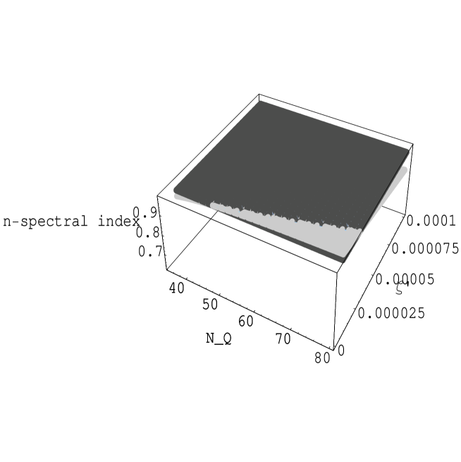
Figure 3:

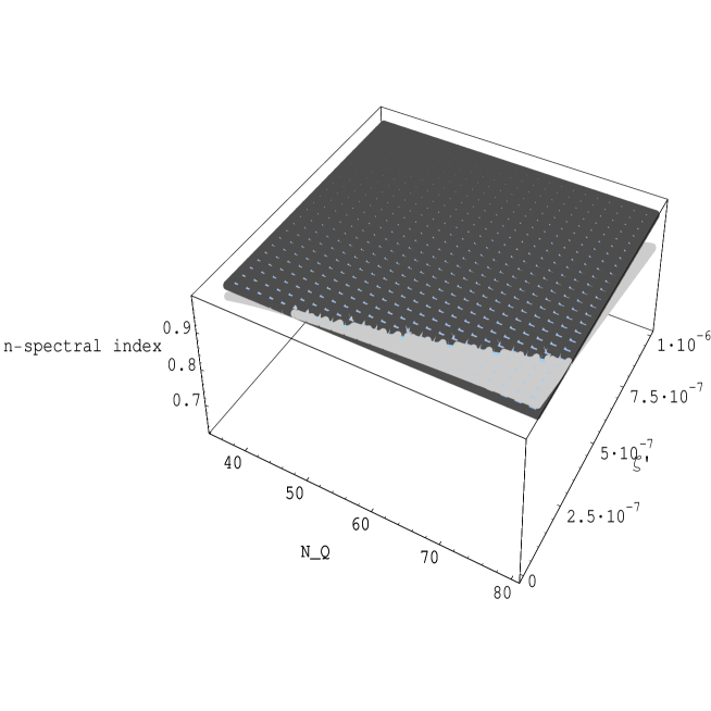
Figure 4:

.

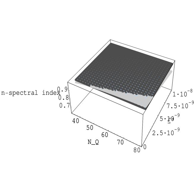
Figure 5:

.

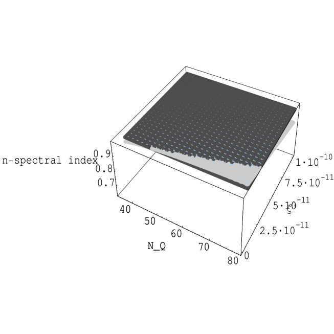
Figure 6:

.

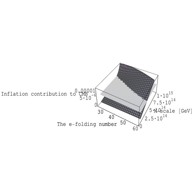
Figure 7:

Figure captions

Fig 1: The spectral index $n$ as a function of the number of e-folding $N(S_{Q})$. Two lines present the bound of the spectral index by WMAP collaboration five year data given in (55)

Fig 2: The inflationary contribution to the quadrupole as a function of $\frac{M_{X}}{M_{P}}$

Fig 3: The spectral index $n$ as a function of the number of e-folding $N(S_{Q})$ and $\zeta$, taking $\alpha=10^{-3}$. The gray plane presents the bound of the spectral index by the five-year WMAP data given in (55)

Fig 4: The spectral index $n$ as a function of the number of e-folding $N(S_{Q})$ and $\zeta$, taking $\alpha=10^{-4}$. The gray plane presents the bound of the spectral index by the five-year WMAP data given in (55)

Fig 5: The spectral index $n$ as a function of the number of e-folding $N(S_{Q})$ and $\zeta$, taking $\alpha=10^{-5}$. The gray plane presents the bound of the spectral index by the five-year WMAP data given in (55)

Fig 6: The spectral index $n$ as a function of the number of e-folding $N(S_{Q})$ and $\zeta$, taking $\alpha=10^{-6}$. The gray plane presents the bound of the spectral index by the five-year WMAP data given in (55)

Fig 7: The inflation contribution to CMB temperature as a function of the number of e-folding $N(S_{Q})$ and $M_{X}$ in the case $\alpha=10^{-6}$ . The light plane presents 90% of the quadrupole measured by COBE given in (57)

References

- (1) See, for example, A. H. Guth, Phys. Rev. D 23, 347 (1981); A. Linde, Phys. Lett. 108 B, 389 (1982); A. Albrecht and P. J. Steinhardt, Phys. Rev. Lett. 48, 1220 (1982).
- (2) A. Linde, Phys. Lett. 129 B, 177 (1983).
- (3) A. Linde, Particle Physics and Inflationary Cosmology, Contemporary Concepts in Physics, Vol. 5 (Harwood Academic, Chur, Switzerland, 1990); H. Ohanian and R. Ruffini, Gravitation and Spacetime, 2nd edition, (W.W. Norton & Company, 1994).
- (4) A. R. Liddle and L. A. Urena-Lopez, Phys. Rev. Lett. 97, 161301 (2006); A. R. Liddle, C. Pahud, and L. A. Urena-Lopez, Phys. Rev. D 77, 121301(R) (2008).
- (5) T. W. B. Kibble, J. Phys. A 9, 1387 (1976); See also Ref. linde1 .
- (6) F. Pisano and V. Pleitez, Phys. Rev. D 46 410 (1992); P. H. Frampton, Phys. Rev. Lett. 69, 2889 (1992); R. Foot et al., Phys. Rev. D 47, 4158 (1993).
- (7) M. Singer et al., Phys. Rev. D 22, 738 (1980).
- (8) R. Foot, H. N. Long and Tuan A. Tran, Phys. Rev. D 50, R34 (1994); J. C. Montero et al., Phys. Rev. D 47, 2918 (1993); H. N. Long, Phys. Rev. D 54, 4691 (1996); H. N. Long, Phys. Rev. D 53, 437 (1996).
- (9) W. A. Ponce, Y. Giraldo, and L. A. Sanchez, Phys. Rev. D 67, 075001 (2003).
- (10) P. V. Dong, H. N. Long, D. T. Nhung, and D. V. Soa, Phys. Rev. D 73, 035004 (2006).
- (11) P. V. Dong and H. N. Long, Advances in High Energy Physics, Vol. 2008, Article ID 739492, 74 pages; doi: 10.1155/2008/739492, [arXiv:0804.3239(hep-ph)](2008).
- (12) P. V. Dong, H. N. Long, and D. V. Soa, Phys. Rev. D 73, 075005 (2006).
- (13) P. V. Dong, Tr. T. Huong, D. T. Huong and H. N. Long, Phys. Rev. D 74, 053003 (2006).
- (14) P. V. Dong, H. N. Long, and D. V. Soa, Phys. Rev. D 75, 073006 (2007).
- (15) See, for example, J. Wess and J. Bagger, Supersymmetry and Supergravity, 2nd edition, Princeton University Press, Princeton NJ, (1992); H. E. Haber and G. L. Kane, Phys. Rep. 117, 75 (1985).
- (16) S. Martin, A supersymmetry primer, [arXiv:hep-ph/9709356].
- (17) A. Brignole, J. A. Casas, J. R. Espinosa and I. Navarro, Nucl. Phys. B 666, 105 (2003); M. Dine, N. Seiberg, and S. Thomas, Phys. Rev. D 76, 095004 (2007), [arXiv:0707.0005](2007).
- (18) J. C. Montero, V. Pleitez, and M. C. Rodriguez, Phys. Rev. D 65, 035006 (2002).
- (19) T. V. Duong and E. Ma, Phys. Lett. B 316, 307 (1993); J. Phys. G 21, 159 (1995); M. C. Rodriguez, Int. J. Mod. Phys. A 21, 4303 (2006).
- (20) J. C. Montero, V. Pleitez, and M. C. Rodriguez, Phys. Rev. D 65, 095008 (2002); C. M. Maekawa and M. C. Rodriguez, JHEP 04, 031 (2006).
- (21) M. Capdequi-Peyranere, M. C. Rodriguez, Phys. Rev. D 65, 035001 (2002).
- (22) H. N. Long and Palash B Pal, Mod. Phys. Lett. A 13, 2355 (1998).
- (23) J. C. Montero, V. Pleitez, and M. C. Rodriguez, Phys. Rev. D 70, 075004 (2004).
- (24) D. T. Huong, M. C. Rodriguez and H. N. Long, Scalar sector of supersymmetric model with right-handed neutrinos, [arXiv:hep-ph/0508045].
- (25) P. V. Dong, D. T. Huong, M. C. Rodriguez, and H. N. Long, Eur. Phys. J. C 48, 229 (2006), [arXiv: hep-ph/0604028 ].
- (26) P. V. Dong, D. T. Huong, M. C. Rodriguez, and H. N. Long, Nucl. Phys. B 772, 150 (2007).
- (27) P. V. Dong, D. T. Huong, N. T. Thuy, and H. N. Long, Nucl. Phys. B 795, 361 (2008).
- (28) P. V. Dong, Tr. T. Huong, N. T. Thuy, and H. N. Long, JHEP 11, 073 (2007).
- (29) D. T. Huong and H. N. Long, JHEP 07, 049 (2008), [arXiv:0804.3875(hep-ph)](2008).
- (30) R. Jeannerot, Phys. Rev. D 56, 6205 (1997).
- (31) D. Chang, H. N. Long, Phys. Rev. D 73, 053006 (2006).
- (32) E. J. Copeland, A. R. Liddle, D. H. Lyth, E. D. Stewart, and D. Wands, Phys. Rev. D 49, 6410 (1994).
- (33) G. Dvali, Q. Shafi and R. Schaefer, Phys. Rev. Lett. 73, 1886 (1994).
- (34) A.Linde and A. Riotto, Phys. Rev. D 56, 1841 (1997).
- (35) V. Nefer Senoguz and Q. Shafi, Phys. Lett. B 668, 6 (2008), [arXiv:0806.2798(hep-ph)](2008).
- (36) S. Coleman and S. Weinberg, Phys. Rev. D 7, 1888 (1973).
- (37) Q. Shafi and V. N. Senoguz, Phys. Rev. D 73, 127301 (2006).
- (38) D. H. Lyth and A. Riotto, Phys. Rep. 314, 1 (1999).
- (39) A. R. Liddle and D. H. Lyth, Cosmological Inflation and Large-Scale Structure, Cambridge University Press, (2000).
- (40) J. Dunkley, et al. [WMAP Collaboration], Five-Year Wilkinson Microwave Anisotropy Probe (WMAP) Observations: Angular Power Spectra, [arXiv:0803.0586(astro-ph)](2008); E. Komatsu, et al. [WMAP Collaboration], Five-year Wilkinson Microwave Anisotopy Probe Observations: Cosmological Interpretation, [arXiv:0803.0547(astro-ph)](2008).
- (41) C. L. Bennett et al., Astrophys. J. Suppl. 148, 1 (2003), [arXiv:astro-ph/0302207] D. N. Spergel et al. [WMAP Collaboration], Astrophys. J. Suppl. 148, 175 (2003),[arXiv: astro-ph/0302209]
- (42) D. N. Spergel et al. [WMAP Collaboration], Astrophys. J. Suppl. 170, 377 (2007), [arXiv: astro-ph/0603449]; L. Pogosian, I. Wasserman, and M. Wyman, [arXiv:astro-ph/0604141].
- (43) E. Cremmer et al, Phys. Lett. B 79 , 231 (1978), Nucl. Phys. B 147, 105 (1979), J. Barger, Nucl. Phys. B 211, 302 (1983).
- (44) R. Jeannerot and M. Postma, JHEP 0505, 071 (2005).
- (45) M. Bastero-Gil, S. F. King and Q. Shafi, Phys. Lett. B 651, 345 (2007).
.
.
.