Precision shooting: Sampling long transition pathways

Abstract

The kinetics of collective rearrangements in solution, such as protein folding and nanocrystal phase transitions, often involve free energy barriers that are both long and rough. Applying methods of transition path sampling to harvest simulated trajectories that exemplify such processes is typically made difficult by a very low acceptance rate for newly generated trajectories. We address this problem by introducing a new generation algorithm based on the linear short-time behavior of small disturbances in phase space. Using this “precision shooting” technique, arbitrarily small disturbances can be propagated in time, and any desired acceptance ratio of shooting moves can be obtained. We demonstrate the method for a simple but computationally problematic isomerization process in a dense liquid of soft spheres. We also discuss its applicability to barrier crossing events involving metastable intermediate states.

I Introduction

Transition path sampling (TPS) is a versatile and efficient set of computational techniques for the study of rare events.Dellago et al. (1998); Dellago et al. (2002a); Dellago et al. (2006); Dellago et al. (2002a) It has been successfully used to reveal the microscopic mechanisms of processes as diverse as autoionization in liquid water Geissler et al. (2001), structural transformations in nanocrystalline solids Grünwald et al. (2007), and folding of small proteins.Bolhuis and Juraszek (2006) The purpose of this paper is to propose a new shooting algorithm which can greatly increase the efficiency of TPS when transit times of activated trajectories greatly exceed the picosecond time scale of phase space stability.

At its core TPS is a Monte Carlo procedure enabling a random walk in the ensemble of pathways that cross a free energy barrier between two metastable states (denoted A and B). While this sampling is strongly biased towards reactive trajectories, it leaves the underlying dynamics of the system unchanged. Thus, the result of a TPS simulation is a representative set of true dynamical pathways, weighted as if they were excerpted from an extremely long, unbiased simulation of equilibrium dynamics. Many analytical tools have been developed to extract from such a collection of trajectories useful molecular information about the process of interest.Dellago et al. (2002a)

The algorithm typically used to construct such a random walk is called shooting Dellago et al. (2002a). Here, a point along a given reactive trajectory is randomly selected and slightly changed; for instance, one might change the velocities of all particles by a small random number drawn from a symmetric distribution. Using the dynamical rules of the system, this shooting point is then propagated forward and backward in time to obtain a complete new trajectory. If this new trajectory still connects A with B it is accepted and used as a basis for the next shooting move; otherwise it is rejected.

The efficiency of this algorithm in exploring the transition path ensemble is based on a balance between the intrinsic instability of complex dynamical systems and the local character of the shooting move: Small disturbances grow exponentially quickly in time, leading to separation of trajectories typically within a few picoseconds. Nonetheless, if the disturbance is small, the new trajectory will be locally similar to the old one and is therefore likely to surmount the barrier between A and B; such shooting moves will be accepted frequently. Just as with conventional Monte Carlo moves in configuration space, maximum efficiency can often be obtained by adjusting the size of the disturbance to achieve an acceptance probability of roughly 40%. Dellago et al. (2002a)

Shooting moves are best suited for the study of systems that relax quickly (within the picosecond time scale of trajectory separation) into their product state after reaching the top of the barrier. Many interesting processes, like the nucleation of first order phase transitions or conformational change in complex molecules, proceed much more slowly from the transition state. In TPS simulations of such systems, shooting moves must be made extraordinarily subtle in order to stand a reasonable chance of connecting reactant and product states. As a matter of practice, however, disturbances cannot be made arbitrarily small due to the limited machine precision of floating point numbers. Lacking an ability to control the degree of global separation between trajectories, TPS methods are severely compromised in efficacy. The demonstrated computational advantages of importance sampling in trajectory space lose appeal when offset by the wasted effort of generating a vast excess of non-reactive paths.

In a recent paperBolhuis (2003), Bolhuis addressed this problem by modifying slightly the rules that propagate a system in time. Specifically, a weak stochastic component was added to the dynamics, removing the unique correspondence between a trajectory’s past and its future. It thus became possible to resample only parts of an existing pathway, leading to much higher acceptance probabilities for shooting moves and, Bolhuis reports, significant improvement in sampling efficiency.Bolhuis (2003)

In this paper, we show that it is possible to perform productive shooting moves for arbitrarily long transition paths without modifying a system’s natural dynamics. Our technique for introducing and propagating extraordinarily small disturbances is based on the simple dynamics of small perturbations in phase space. We explain the method and offer a straightforward algorithm for implementation in Sec. II. Use of the technique is demonstrated in Sec. III for a simple isomerization process in a dense liquid that, by construction, involves diffusive dynamics on a rugged barrier. In Sec. IV we examine limitations of the method by considering reactive dynamics that pass through highly metastable, obligatory intermediate states.

II Linearized dynamics of small perturbations

II.1 Exponential divergence of trajectories

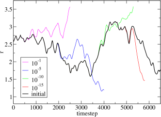
Figure 1: Distance $r$, in reduced units, between two particles in a liquid of 108 soft spherestestsys as a function of time along a reference trajectory and four shooting trajectories. At time zero, displacements of various size are added to particle velocities in the reference trajectory. Because phase space disturbances grow exponentially in time, decreasing the shooting displacement by successive orders of magnitude results in only linear increase in the time that elapses before trajectories separate. Shooting displacements smaller than $10^{-15}$ can not be resolved in double precision; the resulting shooting trajectories will exactly retrace the initial one.

In a TPS simulation of a system evolving with deterministic dynamics, a trajectory $X$ of length $\tau$ consists of a number of “snapshots” $x_{i\Delta t}$, which are separated by a time step $\Delta t$,

$$X=\{x_{0},x_{\Delta t},x_{2\Delta t},\dots,x_{\tau}\}\;.$$ (1)

Here, the time slices $x_{i\Delta t}$ are full phase space vectors, detailing the positions and velocities of all particles. Subsequent time slices are related by

$$x_{(i+1)\Delta t}=\Phi(x_{i\Delta t})\;,$$ (2)

where the function $\Phi$ propagates the system for one time step.

Consider now a shooting move, in which a small disturbance $\delta x_{0}$ is added to the shooting point $x_{0}$ to obtain state $y_{0}=x_{0}+\delta x_{0}$ of the shooting trajectory $Y$. (To simplify notation, we will assume the shooting point to be $x_{0}$, the initial state of the trajectory, throughout this section. The algorithm we will describe applies transparently to shooting points at any chosen time along the trajectory.) Usually the perturbation $\delta x_{0}$ affects only momentum space, but changing the positions of the particles can be useful in some cases Dellago et al. (2002a). The perturbed point $y_{0}$ is then propagated for a number of $n$ time steps to obtain $y_{t}=\Phi_{t}(y_{0})$, where $t=n\Delta t$ and $\Phi_{t}$ refers to the $n$-fold application of the time step propagator. We define the time-evolved disturbance $\delta x_{t}$ by subtracting the old trajectory from the new one, $\delta x_{t}=y_{t}-x_{t}$. Due to the dynamic instability of the system, perturbations grow exponentially in time,

$$|\delta x_{t}|\approx|\delta x_{0}|\,e^{\lambda t}\;.$$ (3)

Here, $\lambda$ is the largest Lyapunov exponent of the system.Posch and Hoover (1989) For typical fluid systems, $1/\lambda\approx 1\,\mathrm{ps}$.

We wish to control precisely the time it takes for a small perturbation to reach a size of order 1, at which point the new trajectory will be essentially separated from the old one. This time determines the probability that the new trajectory will be reactive and therefore acceptable. Because of subsequent exponential growth, $|\delta x_{0}|$ must be decreased by many orders of magnitude to increase the separation time of trajectories by even a few picoseconds (see Figs. 1 and 2). With the standard double precision format for representing floating point numbers on a computer, however, the smallest number that can be added to 1.0 to give a result distinguishable from 1.0 is of the order of $10^{-15}$, and numerical results become unreliable at values of $|\delta x_{0}|$ well above this limit. (We assume throughout this paper that a system of units has been chosen such that typical numerical values of coordinates and momenta are of order 1.) Especially when the total length of the transition path is significantly longer than a few picoseconds, the limited range of practical displacement sizes constitutes a severe sampling problem: Shooting moves will only be accepted from points in the vicinity of the barrier top; otherwise, new trajectories will simply return to the stable state they came from and be rejected. As the system may stay near the a priori unknown barrier top only for a small fraction of the total transition time, sampling can break down completely. In these cases, implementing shooting displacements of arbitrarily small size would be very helpful.

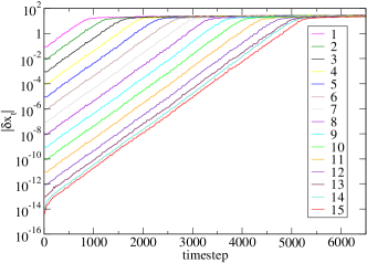
Figure 2: Time evolution of small displacements $\delta x_{t}$ in a liquid of 108 soft spherestestsys for disturbances of various sizes, $|\delta x_{0}|=10^{-\alpha}$ (legend values indicate values of $\alpha$). All displacements grow exponentially with the same rate, up to the time where trajectories separate. The maximum possible value of $|\delta x_{t}|$ is determined by the dimensions of the simulation box. Note that adjacent lines are equidistant in the linear regime, except for displacement sizes smaller than $10^{-12}$. Although these smallest displacements yield trajectories that can in practice be distinguished from the base trajectory, limited numerical precision introduces rounding errors that degrade computational estimates of linear divergence.

II.2 Dynamics in the linear regime

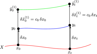
Figure 3: Time evolution of shooting moves from a point $x_{0}$ on the reference trajectory $X$. The two shooting displacements $\delta x_{0}$ and $\delta\hat{x}_{0}^{(1)}$, as vectors in high-dimensional phase space, point in the same direction but have different magnitudes, $\delta\hat{x}_{0}^{(1)}=c_{0}\,\delta x_{0}$. At a later time $t$ short enough that first-order perturbation theory remains valid, these displacements remain proportional, $\delta x_{t}^{(1)}=c_{0}\,\delta x_{t}$. The displacement of interest $\delta x_{t}$, no matter how small, can thus be constructed in the linear regime simply by dividing $\delta\hat{x}_{t}^{(1)}$ by the original scaling factor $c_{0}$.

We propose to solve this problem by using perturbation theory to follow the time evolution of the displacement vector $\delta x_{0}$ itself, up to the point where it grows large enough to allow accurate evaluation of the sum $x_{t}+\delta x_{t}$. Expanding $y_{t}$ around $x_{0}$, we obtain

$$\delta x_{t}=y_{t}-x_{t} = \Phi_{t}(x_{0}+\delta x_{0})-\Phi_{t}(x_{0})=$$ (4)

$$= \frac{\partial\Phi_{t}(x_{0})}{\partial x_{0}}\,\delta x_{0}+\mathcal{O}\left[(\delta x_{0})^{2}\right]\;.$$

For small displacements $|\delta x_{0}|<10^{-15}$, the linear approximation is for all practical purposes exact on the scale of a single time step,

$$\delta x_{t}=S\,\delta x_{0}\;,$$ (5)

where the matrix $S$ is given by

$$S=\frac{\partial\Phi_{t}(x_{0})}{\partial x_{0}}\;.$$ (6)

To integrate $\delta x_{0}$ forward in time according to equation (5), the equations of motion for the matrix $S$ could in principle be solved numerically.Dellago et al. (1996b) Doing so in practice would be cumbersome, requiring calculation of all second derivatives of the interaction potential with respect to particle positions. We propose a much simpler approach for advancing $\delta x_{t}$, inspired by methods for computing Lyapunov exponents in systems whose interaction potentials lack well-defined second derivatives. Our implementation is illustrated in Fig. 3.

Instead of integrating the small perturbation $\delta x_{0}$, we follow the time evolution of a related perturbation $\delta\hat{x}_{0}^{(1)}$, which is large enough to be added at the shooting point and propagated in the usual way, i.e., by integrating Newton’s equation of motion for $\hat{y}_{0}^{(1)}=x_{0}+\delta\hat{x}_{0}^{(1)}$. We use a superscript for $\hat{y}^{(i)}$ and $\delta\hat{x}^{(i)}$ because in the following we will consider a family of different perturbed trajectories $\hat{Y}^{(i)}=\{\hat{y}_{0}^{(i)},\dots,\hat{y}_{\tau}^{(i)}\}$, with $\hat{y}_{t}^{(i)}=x_{t}+\delta\hat{x}_{t}^{(i)}$. Exploiting the linearity described by Eq. (5), we choose $\delta\hat{x}_{0}^{(1)}$ to be in the same direction (in the high-dimensional phase space) as $\delta x_{0}$,

$$\delta\hat{x}_{0}^{(1)}=c_{0}\,\delta x_{0}\;,$$ (7)

where $c_{1}$ is a scalar constant. If $\delta\hat{x}_{0}^{(1)}$ is also small enough to justify the linear approximation of Eq. (5),

$$\delta\hat{x}_{t}^{(1)}=S\,\delta\hat{x}_{0}^{(1)}\;,$$ (8)

then the initial relationship between $\delta x_{0}$ and $\delta\hat{x}_{0}^{(1)}$ holds also at a later time $t$,

$$\delta x_{t}=S\,\delta x_{0}=\frac{1}{c_{0}}\,S\,\delta\hat{x}_{0}^{(1)}=\frac{1}{c_{0}}\,\delta\hat{x}_{t}^{(1)}\;.$$ (9)

In the linear regime it is thus possible to follow the time evolution of arbitrarily small displacements $\delta x_{0}$ by monitoring larger, proportional displacements.

The linear approximation for the “helper” displacement $\delta\hat{x}_{t}^{(1)}$ in Eq. (8) will of course remain valid for only a short time $t_{\rm lin}^{(1)}$, typically less than 1 ps. Our interest in the trajectory $\hat{Y}^{(1)}$, however, is only as a proxy for the evolution of smaller displacements that cannot be represented explicitly. As $\delta\hat{x}_{t}^{(1)}$ approaches the boundary of the linear regime, $t\raisebox{-2.15277pt}{$\>\stackrel{{\scriptstyle\textstyle<}}{{\sim}}\>$}t_{\rm lin}^{(1)}$, we may therefore switch our attention to a different helper trajectory $\hat{Y}^{(2)}$, one whose displacement is initially too small to be of practical use but by the time $t_{\rm lin}^{(1)}$ grows large enough to be represented explicitly. The new displacement $\delta\hat{x}_{t}^{(2)}=\hat{y}_{t}^{(2)}-x_{t}$ can be obtained at any time $t<t_{\rm lin}^{(1)}$ simply by scaling $\delta\hat{x}_{t}^{(1)}$ appropriately, $\delta\hat{x}_{t}^{(2)}=\delta\hat{x}_{t}^{(1)}/c_{1}$. Because it is initially smaller than $\delta\hat{x}_{t}^{(1)}$, it will remain in the linear regime for a longer time, $t_{\rm lin}^{(2)}>t_{\rm lin}^{(1)}$. For times $t>t_{\rm lin}^{(1)}$ we therefore proceed by integrating standard equations of motion for $\hat{Y}^{(2)}$ until it approaches the boundary of the linear approximation. At that point we repeat the procedure, scaling back the displacement to switch attention to yet another helper trajectory.

In effect we monitor a single displacement from the reference trajectory whose magnitude is periodically scaled down such that the linear approximation is always valid. In this way we can monitor the time evolution of an arbitrarily small disturbance. The corresponding trajectory will be numerically indistinguishable from the reference trajectory as long as the displacement’s magnitude is smaller than $\sim 10^{-15}$. At later times the displaced trajectory can be distinguished, and its dynamics can be safely computed by integrating equations of motion in the usual way.

II.3 Algorithm

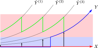
Figure 4: Precision shooting algorithm for generating a trial trajectory $Y$ (blue curve) whose initial displacement from the base trajectory $X$ (red line) is extraordinarily small. Points in the light blue field (whose extent is $\approx 10^{-15}$) cannot be numerically distinguished from the reference trajectory. Until the trial trajectory exits this region, its time evolution is calculated by proxy using “helper” trajectories $\hat{Y}^{(i)}$ (thin black curves). Displacements of trial (black arrows) and helper trajectories from the base trajectory are related by proportionality as long as they remain within the linear regime, represented by the light red field. To preserve this simple relationship, the displacement of the helper trajectory $\hat{Y}^{(i)}$ from the reference trajectory is scaled back when it threatens to leave the region of linear dynamics, effectively switching the system to the next helper trajectory $\hat{Y}^{(i+1)}$. By following the systems dynamics along many sections of helper trajectories (green curve) and by keeping track of the rescaling factors, one can accurately construct the state of the trial trajectory once it becomes distinguishable from the reference trajectory. The result of this shooting move is a trial trajectory $Y$ that is numerically identical to the base trajectory $X$ over a certain length of time and then emerges from it in the correct way.

This insight suggests the following algorithm, which implements a shooting trajectory $Y$, whose initial deviation $\delta x_{0}$ from the base-trajectory $X$ is smaller than the precision limit. This is done by monitoring “helper” trajectories $\hat{Y}^{(j)}$, which are obtained by repeated rescaling. For an illustration of this algorithm see Fig. 4.

1. At the shooting point $x_{0}$, add a displacement $\delta\hat{x}_{0}^{(1)}$ of fixed size $|\delta\hat{x}_{0}^{(1)}|=\sigma$. The displacement $\delta\hat{x}_{0}^{(1)}$ is parallel to $\delta x_{0}$ and larger by a factor of $c_{0}$.

2. Propagate the point $\hat{y}_{0}^{(1)}=x_{0}+\delta\hat{x}_{0}^{(1)}$ forward in time for $n$ time steps, corresponding to a time interval $t=n\Delta t$.

3. Compute the factor $c_{1}=|\delta\hat{x}_{t}^{(1)}|/|\delta\hat{x}_{0}^{(1)}|=|\hat{y}_{t}^{(1)}-x_{t}|/|\delta\hat{x}_{0}^{(1)}|$ quantifying the divergence from the reference trajectory. Switch to a new helper trajectory by setting $\hat{y}_{t}^{(2)}=x_{t}+\delta\hat{x}_{t}^{(1)}/c_{1}=x_{t}+\delta\hat{x}_{t}^{(2)}$. Store the factor $c_{1}$.

4. Propagate the new displacement forward in time by integrating the equations of motion for $n$ steps beginning from $\hat{y}_{t}^{(2)}$. Calculate and store the factor $c_{2}=|\delta\hat{x}_{2t}^{(2)}|/|\delta\hat{x}_{t}^{(2)}|$.

5. Iterate step 4, each time beginning from $\hat{y}_{(j-1)t}^{(j)}$ and rescaling by the factor $c_{j}=|\delta\hat{x}_{jt}^{(j)}|/|\delta\hat{x}_{(j-1)t}^{(j)}|$. At every iteration compute the displacement of interest, $\delta x_{jt}=C_{j}^{-1}\,\delta\hat{x}_{jt}^{(j)}$, where $C_{j}=\Pi_{k=0}^{j-1}c_{k}$ is the product of all factors used for rescaling so far. To store the current point along the actual shooting trajectory, compute $y_{jt}=x_{jt}+\delta x_{jt}$. As long as $|\delta x_{jt}|\lesssim 10^{-15}$, $y_{jt}$ will be numerically identical to $x_{jt}$.

6. If $|\delta x_{jt}|>\sigma$, the actual shooting displacement is large enough to be treated in the usual way: Set $y_{jt}=x_{jt}+\delta x_{jt}$ and integrate equations of motion from this point without further rescalings (ceasing iteration of step 4).

Note that for shooting moves conducted at points other than $x_{0}$, the procedure must be repeated backward in time to obtain a complete shooting trajectory. In the following we discuss the accuracy of this scheme and give recommendations for choosing values of $\sigma$ and $n$.

II.4 Validity of the linear approximation

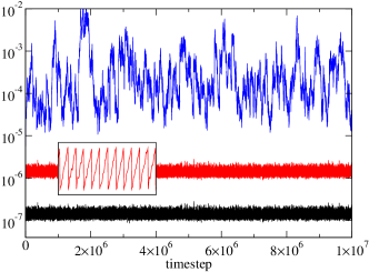
Figure 5: Time evolution of the magnitude of two shooting displacements for a fluid of WCA particles.testsys Displacements of size $|\delta\hat{x}_{0}^{(1)}|=10^{-7}$ (black) and $|\delta\hat{x}_{0}^{(2)}|=10^{-6}$ (red) are initially proportional (pointing in the same direction in phase space). Both are rescaled to their initial size every 100 time steps (see inset for a magnified view) to preserve this linear relationship. Deviation from proportionality is quantified by the relative error $\epsilon(t)$ (blue) defined in Eq. (10).

The above algorithm is exact only if the linear approximation of Eq. (5) holds. For perturbations of finite size, deviations from this approximation occur. The question thus arises, how accurate an approximation is this approach for propagating small disturbances? More specifically, to what extent do helper displacements remain proportional to the actual shooting displacements of interest? One could certainly imagine that the fast growth of small non-linearities rapidly erodes the linear relationship on which we depend. Here we present evidence from computer simulations that proportionality of small displacements can hold in practice over very long time scales.

Figure 5 shows the time evolution of two proportional disturbances. The initial displacement vectors point in the same direction of phase space but have different magnitudes, $|\delta\hat{x}_{0}^{(1)}|=10^{-7}$ and $|\delta\hat{x}_{0}^{(2)}|=10^{-6}$. The respective shooting trajectories were propagated independently, and the displacements from the base trajectory were rescaled to their initial length every 100 time steps. For a perfectly linear time evolution, these displacements remain proportional at all later times. In practice the vectors $\delta\hat{x}_{t}^{(1)}$ and $\delta\hat{x}_{t}^{(2)}$ will develop a nonzero angle due to non-linearities. To quantify this deviation from parallel alignment, we define

$$\epsilon(t)=\frac{|\delta\hat{x}_{t}^{(1)}-\delta\hat{x}_{t}^{(2)}/10|}{|\delta\hat{x}_{t}^{(1)}|}\,.$$ (10)

As shown in Fig. 5, the relative error $\epsilon(t)$ does not grow above a low level even for very long simulation runs.

This long time stability of aligned disturbances holds over a broad range of displacement sizes between $10^{-10}$ and $10^{-3}$. Values of $\epsilon(t)$ can be somewhat larger than for the specific case plotted in Fig. 5 but on average do not grow larger than $10^{-3}$ for any case. The error is insensitive to the choice of the rescaling interval $n\Delta t$, as long as the displacements stay smaller than approximately $10^{-2}$, where the linear regime breaks down. For displacements smaller than $10^{-10}$, rounding errors become problematic, and phase space displacements do not remain parallel to a good approximation. One might expect the region of long time stability to extend to even lower levels, closer to the precision limit of $10^{-15}$. However, the total achievable accuracy in a computer simulation depends, among other factors, on the details of the integrator $\Phi$, the size of the time step, and the dimensionality of the system, and can lie well above the precision limit of $10^{-15}$. We find that for the particular system used here, the precision level is about $10^{-12}$.

In the light of these observations, a value of $\sigma=10^{-6}$ as initial magnitude for helper displacements seems appropriate. This choice lies midway between the upper limit of the linear regime (approximately $10^{-2}$), and the point where rounding errors become dominant (approximately $10^{-10}$). As the accuracy of the rescaling scheme is quite insensitive to the frequency of rescalings, many equally good choices of $n$ are possible. As a starting point, a value of $n$ which leads to rescalings every time the displacements have doubled their size is advisable.

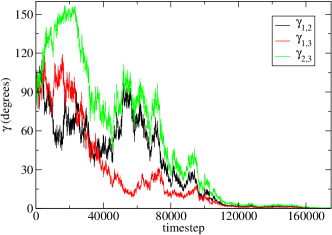
Figure 6: Relative orientations of three phase space displacement vectors ($\delta\hat{x}_{t}^{(1)}$, $\delta\hat{x}_{t}^{(2)}$, and $\delta\hat{x}_{t}^{(3)}$) for a WCA fluid.testsys We plot the angle $\gamma_{i,j}=\cos^{-1}(\delta\hat{x}_{t}^{(i)}\cdot\delta\hat{x}_{t}^{(j)}/|\delta\hat{x}_{t}^{(i)}||\delta\hat{x}_{t}^{(j)}|)$ between each pair of displacements as a function of time. Displacements differ in initial direction and size ($|\delta\hat{x}_{0}^{(1)}|=10^{-8}$, $|\delta\hat{x}_{0}^{(2)}|=10^{-8}$, $|\delta\hat{x}_{0}^{(3)}|=10^{-7}$) and are rescaled to their original sizes at different intervals ($n_{x}=100$, $n_{y}=200$, $n_{z}=500$).

The fact that $\epsilon(t)$ does not show any systematic long-time growth in Fig. 5 seems surprising. After all, no constraint is imposed on the direction of the displacement vectors. Why does an accumulation of errors not eventually lead to decoupling and $\epsilon(t)\approx 1$? Stability of the precision shooting algorithm is in fact a simple and direct consequence of the collective dynamics of displacements in the linear regime. In Figure 6 we plot the angles between three periodically rescaled shooting displacement vectors of different size and random initial direction. Eventually, they all rotate into the same direction, which is associated with the largest Lyapunov exponent $\lambda$ of the system. The time scale on which the directions of different displacement vectors converge is on the order of $1/\Delta\lambda$, where $\Delta\lambda$ is the difference between the first and second largest Lyapunov exponents.Dellago et al. (2002b) It is because of this convergence, that the difference vector $\delta\hat{x}_{t}^{(1)}-\delta\hat{x}_{t}^{(2)}/c$ between two proportional displacements with initially identical direction will stay small.

We point out that this property constitutes a main difference of our method over the stochastic scheme introduced by BolhuisBolhuis (2003) and similar algorithms. Consider, for instance, the following simple algorithm that can be viewed as a smooth version of the stochastic scheme by Bolhuis:

• Choose a shooting point $x_{\mathrm{s\Delta t}}$.

• A fixed number of timesteps $n$ earlier and later, at the points $x_{(s+n)\Delta t}$ and $x_{(s-n)\Delta t}$, add a displacement of $10^{-15}$ to one velocity component of one particle.

• Integrate the points $x_{(s+n)\Delta t}$ and $x_{(s-n)\Delta t}$ forward and backward in time, respectively, to get a complete new trajectory.

Just like the precision shooting algorithm, this simple scheme results in a shooting trajectory that is numerically identical to its base trajectory for a certain period of time. However, the emerging separation between base and shooting trajectories will not be consistent with a shooting move conducted at $x_{0}$, but rather with two uncorrelated shooting moves at $x_{(s+n)\Delta t}$ and $x_{(s-n)\Delta t}$. Our algorithm, on the other hand, correctly reproduces the correlated forward and backward dynamics of a displacement introduced at $x_{s\Delta t}$.

III A simple test system

We demonstrate the precision shooting algorithm on a simple isomerization process of a solvated diatomic molecule in three dimensions.

Our test system consists of 389 particles interacting via the WCAWeeks et al. (1971) potential. We use conventional reduced units, with particle mass and potential parameters $\sigma$ and $\epsilon$ all set to unity. Particles #1 and #2 do not interact via the WCA potential, but are bonded through a one-dimensional potential with two deep minima separated by a rough barrier (see Fig. 7):

$$v(x)=\left\{\begin{array}[]{ll}h_{1}\left[1-q(x)^{2}/w^{2}\right]^{2}&\quad\mathrm{if}\;q(x)<0\,,\\ h_{1}\left[1-(q(x)-b)^{2}/w^{2}\right]^{2}&\quad\mathrm{if}\;q(x)>b\,,\\ h_{1}+h_{2}\frac{\cos^{2}\left[a(q(x)-b/2)\right]}{\sqrt{1+ga^{2}(q(x)-b/2)^{2}}}&\quad\mathrm{else}\,.\end{array}\right.$$ (11)

Here, $q(x)=x-(r_{c}+w)$, $x=x_{2}-x_{1}$ is the difference between the $x$-component of the position of the bonded particles, $r_{c}=2^{1/6}$ is the cutoff of the WCA potential, $w=1$ determines the width of the minima, $b=10$ and $h_{1}=10$ are the length and height of the barrier in between, respectively, and the constants $h_{2}=3$, $a=7\pi/b$, and $g=2$ determine the shape of the barrier. The potential and its derivative are continuous by construction.

Figure 7: Potential energy $v(x)$ of interaction between particles #1 and #2, comprising the diatomic molecule in our model isomerization process, plotted as a function of the difference $x=x_{2}-x_{1}$ between their $x$-coordinates. The dashed lines mark the boundaries of the minima A and B.

To speed computation, we borrow a trick from Bolhuis’ work: Bolhuis (2003) Particle #2 is considered to lie always to the right of particle #1, hence $x>0$. This choice, together with the one-dimensionality of $v(x)$, allows us to choose a simulation box with dimensions $14.4\times 6\times 6$. The resulting particle density is 0.75, the total energy per particle is 1.0, and the temperature is 0.45, as gauged by average kinetic energy. We use the velocity Verlet algorithmFrenkel and Smit (2002) to integrate the equations of motion with a time step of 0.002.

Figure 8: Distribution of transition times $T$ for our model isomerization process, as gauged from 2500 trajectories initiated at the barrier top. Inset: Difference $x=x_{2}-x_{1}$ between the $x$-coordinates of particles #1 and #2 as a function of time for a typical trajectory.

We are interested in sampling the transition of the dimer from the “contracted” minimum A at $x_{\mathrm{A}}=r_{\mathrm{c}}$ to the “extended” minimum B at $x_{\mathrm{B}}=r_{\mathrm{c}}+b+2w$. The dimer is defined to be in state A for $x<x_{\mathrm{A}}+0.75w$ and in state B for $x>x_{\mathrm{B}}-0.75w$ (see Fig. 7). Because the system is dense, and the barrier is both long and rough, relaxation from the transition state into either stable minimum is quite protracted.

In conducting TPS simulations it is important that sampled trajectories are not shorter than typical spontaneous barrier-crossing events.Dellago et al. (2002a) We determine this typical duration for our simple model system by initiating many straightforward molecular dynamics simulations with the dimer bond length set at $x=r_{\mathrm{c}}+w+b/2$, corresponding to the middle of the barrier. Integrating the equations of motion forward and backward in time yields a representative sample of the transition path ensemble. For a particular trajectory, the transition time $T$ is the time the system spends between regions A and B. The resulting distribution of transition times is plotted in Fig. 8. For TPS simulations, we choose a total trajectory length of $3\times 10^{5}$ time steps, long enough to include 98% of the natural transition path ensemble. The bias of our sampling to short transitions is therefore minor.

Although the artificial potential energy landscape studied here does not directly represent any physical system of interest, it nevertheless shares with many real systems features that lead to long transition pathways and make straightforward application of TPS methods ineffective. In our view roughness of the barrier region is an important ingredient. Models featuring long but flat barriers, such as that of Ref. Bolhuis (2003), should not in fact pose any severe problems for path sampling via the standard shooting move. Assuming that motion atop such a flat barrier is diffusive in nature, and that time evolution from the edge of the barrier proceeds into the adjacent minimum with near certainty, then a trajectory initiated on the barrier will relax into stable state A with probability $p_{\mathrm{A}}=1-y/b$, where $y$ is the initial distance from A and $b$ is the width of the barrier. Similarly, the probability of relaxing first into state B is $p_{\mathrm{B}}=y/b$. A standard shooting move from the barrier region then yields a reactive trajectory with probability

$$P_{\mathrm{acc}}=\frac{1}{b}\int_{0}^{b}\mathrm{d}y\,p_{\mathrm{A}}p_{\mathrm{B}}=\frac{1}{6}\,.$$ (12)

This value of the acceptance rate should correspond to near optimal sampling of the transition path ensemble.Dellago et al. (2002a) A problematically low acceptance rate would only arise if one were to sample trajectories of insufficient length, i.e., paths shorter than typical spontaneous transitions.

In our TPS simulations, only momenta (and not particle positions) are disturbed in the shooting moves, with each particle’s momentum changed in each direction by an amount drawn from a Gaussian distribution of standard deviation $\Delta p$ (followed by rescaling of all momenta to enforce energy conservation).Dellago et al. (1998) We conduct standard shooting moves with values of $\Delta p$ of $10^{-1}$, $10^{-5}$, and $10^{-10}$, as well as precision shooting moves with $\Delta p$ ranging in size from $10^{-10}$ to $10^{-300}$. The latter are implemented using helper displacements with $\Delta p=10^{-7}$ and are rescaled every time they reach twice their original size. For the system size studied here, the initial magnitudes of the resulting displacement vectors are larger than the corresponding value of $\Delta p$ by a factor of roughly 34 on average. For instance, $\Delta p=10^{-7}$ results in displacement vectors with an initial size of about $|\delta x_{0}|=3.4\times 10^{-6}$. For each set of sampling parameters, we attempt 50,000 Monte Carlo moves in trajectory space. Roughly half of these trial moves are generated by shooting. The other half are generated by a procedure called “shifting”,Dellago et al. (2002a) in which short trajectory segments are added to and subtracted from the ends of an existing path.

Figure 9: Fraction of shooting moves for our model isomerization process that are accepted in long TPS simulations. Acceptance ratios are shown for shooting displacements of various sizes, $\Delta p=10^{-\alpha}$, implemented using the standard shooting algorithm for values of $\alpha$ of 1, 5, and 10, and the precision shooting algorithm for $\alpha\geq 10$. For $\alpha=10$, the result obtained from the precision shooting algorithm (red) is effectively indistinguishable from the one obtained with standard shooting.

Figure 9 shows the fraction of attempted shooting moves that are accepted in TPS simulations of the diatomic isomerization with a rough barrier. While standard shooting moves are accepted with low frequency, any desired acceptance ratio can be obtained by using the precision shooting technique. Figure 10 shows changes in transition time $T$ over the course of two TPS runs with shooting displacements of $\Delta p=10^{-1}$ and $\Delta p=10^{-100}$. A dramatic difference in the efficiency of generating qualitatively different trajectories for the two cases is evident.

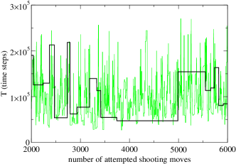
Figure 10: Variation in isomerization transition time $T$ over the course of long TPS runs. The bold black line shows results for a simulation using shooting displacements with $\Delta p=10^{-1}$, while the thin green line corresponds to $\Delta p=10^{-100}$.

To assess the improvement in sampling efficiency achieved with precision shooting, we quantify the computational effort necessary to generate statistically independent transition pathways. More specifically, we calculate the autocorrelation function

$$c(n)=\frac{\langle\delta T(0)\delta T(n)\rangle}{\langle\delta T^{2}\rangle}\,,$$ (13)

where $\delta T(n)=T(n)-\langle T\rangle$ is the deviation of the transition time after the $n$-th shooting move from its average $\langle T\rangle$, as calculated from all collected trajectories.Dellago et al. (2002a); Bolhuis (2003) Rapid decay of $c(n)$ indicates an efficient sampling of trajectories. Figure 11 shows the logarithm of $c(n)$ for different shooting displacement magnitudes along with the “decorrelation time” $\nu$, defined as the number of successive shooting moves after which the correlation function decays to a value less than $1/2$. The maximal sampling efficiency is achieved for shooting displacements with $\Delta p\approx 10^{-100}$. Improvement over the largest displacement we considered ($\Delta p=10^{-1}$) is more than ten-fold. Following BolhuisBolhuis (2003), we also investigate as a measure of decorrelation changes in the bond length $x$ midway in time through the crossing event. Decay of correlations in this quantity, and the implied dependence of sampling efficiency on shooting displacement size, mirror those reported for the transition time $T$.

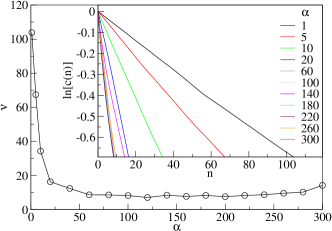
Figure 11: Number of shooting moves required to generate a statistically independent isomerization trajectory using shooting displacements of various sizes, with $\Delta p=10^{-\alpha}$. Inset shows decay of correlation $c(n)$ in the transition time $T$ following $n$ attempted shooting moves. The “decorrelation time” $\nu$ is defined as the value of $n$ beyond which $c(n)<1/2$.

As Fig. 11 illustrates, sampling is comparably efficient for a broad range of displacement sizes between $\Delta p=10^{-60}$ and $\Delta p=10^{-260}$. In this regime, the efficiency gain due to increased acceptance rates for smaller shooting moves is compensated almost exactly by the efficiency loss due to increased similarity between the shooting trajectory and its base trajectory. Using equation (3), the time $T_{\mathrm{id}}$ over which a shooting trajectory with displacement size $10^{-\alpha}$ cannot be resolved from its base trajectory can be approximated by the time required for the displacement size to reach $10^{-15}$,

$$T_{\mathrm{id}}\approx\frac{1}{\lambda_{1}}\ln\frac{10^{-15}}{10^{-\alpha}}=(\alpha-15)\frac{\ln 10}{\lambda_{1}}\,.$$ (14)

For our system, $1/\lambda_{1}\approx 150\,\Delta t$ and therefore $T_{\mathrm{id}}\approx 10^{5}$ time steps for the smallest displacement with $\Delta p=10^{-300}$. Even for this small displacement size, $T_{\mathrm{id}}$ is only 30% of the total trajectory length $L$ and efficient sampling is still possible. If $\delta x_{0}$ is decreased further, $T_{\mathrm{id}}$ will become comparable to $L$ and sampling efficiency will decrease accordingly. For a displacement with $\Delta p=10^{-60}$, the largest size that leads to optimum efficiency, $T_{\mathrm{id}}$ amounts to only 5% of the total trajectory length.

IV Metastable intermediate states

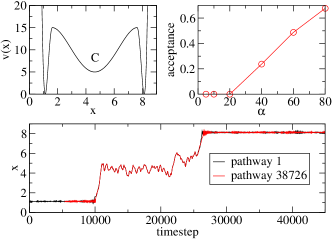
Figure 12: TPS simulation of isomerization dynamics which must proceed through a deep intermediate energy minimum. Top left: Interaction potential between particles #1 and #2. Top right: Acceptance ratio of shooting moves as a function of displacement size, $\Delta p=10^{-\alpha}$. Bottom: Bond length $x$ as a function of time for the starting trajectory and for a pathway obtained after many shooting and shifting moves. The two trajectories have been shifted in time to highlight their similarity in the vicinity of the intermediate state.

By extending the time span over which a shooting trajectory tracks its base trajectory, the algorithm proposed in this work can substantially increase the efficiency of TPS simulations that suffer from poor acceptance of shooting moves. The method is fully consistent with deterministic dynamics and faithfully reproduces the divergent behavior of arbitrarily small displacements in phase space. We emphasize, however, that the method does not solve all problems whose primary symptom is a low shooting acceptance rate. Most importantly, it does not overcome challenges associated with metastable intermediate states. In this section we explore the this difficulty in the context of diatomic isomerization.

In order to explore the consequences of metastable intermediates, we have modified the diatomic potential $v(x)$ to include a deep minimum midway between contracted and extended states (see Fig. 12),

$$v(x)=\left\{\begin{array}[]{ll}h_{1}\left[1-q(x)^{2}/w_{1}^{2}\right]^{2}&\mathrm{if}\;q(x)<0,\\ h_{1}\left[1-(q(x)-2w_{2})^{2}/w_{1}^{2}\right]^{2}&\mathrm{if}\;q(x)>2w_{2},\\ h_{1}-h_{2}\left[1-(q(x)-w_{2})^{2}/w_{2}^{2}\right]^{2}&\mathrm{else}.\end{array}\right.$$ (15)

Here, $q(x)=x-(r_{\mathrm{c}}+w_{1})$, $w_{1}=0.5$, $w_{2}=3$, $h_{1}=15$, and $h_{2}=10$. Limited by machine precision, standard shooting moves fail completely in this case: Even shooting moves initiated near the intermediate minimum C rapidly separate from their base trajectories and with high probability do not escape to stable state A or B. Only with the precision shooting technique, using a displacement size smaller than $10^{-20}$, are we able to conduct successful shooting moves. This success does not indicate, however, that trajectory space is sampled efficiently: A comparison of the first trajectory with a pathway obtained after many thousands of shooting moves shows that those parts of the trajectory spent within the intermediate are not resampled at all (see Fig. 12); they are numerically identical.

Transitions involving strongly metastable intermediates are in fact fundamentally problematic for TPS methods, unless the dynamics of intermediates’ appearance and disappearance can be identified as distinct kinetic substeps. If the typical time spent in C is manageable in a computer simulation, then the intermediate does not pose a problem even to the standard shooting move. If, on the other hand, the free energy barriers delimiting the intermediate state are large compared to typical thermal excitations, then escaping C will itself be a rare event. In such cases, typical transitions from A to B require at least two unlikely fluctuations (activating entry and exit of each intermediate state), well separated in time. Any shooting move that perceptibly modifies dynamics between these rare fluctuations will be rejected with high probability. Precision shooting can readily generate subtly modified pathways that remain reactive but cannot be expected to effectually switch between reactive trajectories that follow substantially different courses through the intermediate state. As TPS leaves a system’s natural dynamics unchanged, it can eliminate only the largest time scale associated with a rare event. Without resorting to methods that prescribe in some sense the detailed route between stable states, one can overcome the challenge of metastable intermediates with TPS only by subdividing transition dynamics into several steps, each of which involves a single dynamical bottleneck.