Polygon Exploration with Time-Discrete Vision

Abstract:

With the advent of autonomous robots with two- and three-dimensional scanning capabilities, classical visibility-based exploration methods from computational geometry have gained in practical importance. However, real-life laser scanning of useful accuracy does not allow the robot to scan continuously while in motion; instead, it has to stop each time it surveys its environment. This requirement was studied by Fekete, Klein and Nüchter for the subproblem of looking around a corner, but until now has not been considered in an online setting for whole polygonal regions.

We give the first algorithmic results for this important optimization problem that combines stationary art gallery-type aspects with watchman-type issues in an online scenario: We demonstrate that even for orthoconvex polygons, a competitive strategy can be achieved only for limited aspect ratio $A$ (the ratio of the maximum and minimum edge length of the polygon), i.e., for a given lower bound on the size of an edge; we give a matching upper bound by providing an $O(\log A)$-competitive strategy for simple rectilinear polygons, using the assumption that each edge of the polygon has to be fully visible from some scan point.

Keywords: Searching, scan cost, visibility problems, watchman problems, online searching, competitive strategies, autonomous mobile robots.

1 Introduction

Visibility Problems: Old and New. The study of geometric problems that are based on visibility is a well-established field within computational geometry. The main motivation is guarding, searching, or exploring a given region (known or unknown) by stationary or mobile guards.

In recent years, the development of real-world autonomous robots has progressed to the point where actual visibility-based guarding, searching, and exploring become very serious practical challenges, offering new perspectives for the application of algorithmic solutions. However, some of the technical constraints that are present in real life have been ignored in theory; taking them into account gives rise to new algorithmic challenges, necessitating further research on the theoretical side, and also triggering closer interaction between theory and practice.

One technical novelty that has lead to new possibilities and demands is the development of high-resolution 3D laser scanners that are now being used in robotics, see Figure 1 for an image and [RAAS2003] for technical details. By merging several 3D scans, the robot Kurt3D builds a virtual 3D environment that allows it to navigate, avoid obstacles, and detect objects [IAS2004]; this makes visibility problems quite practical, as actually using good trajectories is now possible and desirable. However, while human mobile guards are generally assumed to have full vision at all times, Kurt3D has to stop each time it scans the environment, taking in the order of several seconds for doing so; the typical travel time between scans is in the same order of magnitude, making it necessary to balance the number of scans with the length of travel, and requiring a combination of aspects of stationary art gallery problems with the dynamic challenge of finding a short tour.

We give the first comprehensive study of the resulting Online Watchman Problem with Discrete Vision (OWPDV) of exploring all of an unknown region in the presence of a fixed cost for each scan. We focus on the case of rectilinear polygons, which is particularly relevant for practical applications, as it includes almost all real-life buildings. We show that the problem is considerably more malicious in the presence of holes than known for the classical watchman problem; moreover, we demonstrate that even for extremely simple classes of polygons, the competitive ratio depends on the aspect ratio $A$ of the region; practically speaking, this corresponds to the resolution of scans. Most remarkably, we are able to develop an algorithm for the case of simple rectilinear polygons that has competitive ratio $O(\log A)$, which is best possible; this result uses the assumption that each edge of the polygon is fully visibly from some scan point. This assumption has been used before by Bottino and Laurentini [bl-nospabc-08]; in a practical context, it can be justified by avoiding inaccuracies resulting from putting together the individual scans. More importantly, it allows it to sidestep a notorious open problem, which would otherwise come up as a subproblem: finding a small set of stationary guards for a polygonal environment. Details of this and other difficulties of exploration with time-discrete vision are discussed in Section 3.

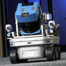
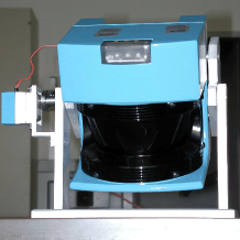
Figure 1: Left: the autonomous mobile robot Kurt3D equipped with the 3D scanner. Right: the AIS 3D laser range finder. Its technical basis is a SICK 2D laser range finder (LMS-200). (Both images used with kind permission by Andreas Nüchter, see [RAAS2003].)

Classical Related Work. Using a fixed set of positions for guarding a known polygonal region is the classical art gallery problem [Chv75, o-agta-87]. Schuchardt and Hecker [sh-tnhag-95] showed that finding a minimum cardinality set of guards is NP-hard, even for a simple rectilinear region; this implies that the offline version of the minimum watchman problem with discrete vision is also NP-hard, even in simple rectilinear polygons.

Finding a short tour along which one mobile guard can see a given region in its entirety is the watchman problem; see Mitchell [joe.survey] for a survey. Chin and Ntafos [chinta88] showed that such a watchman route can be found in polynomial time in a simple rectilinear polygon, while others [thi-iacsw-93, thi-ciacs-99, cjn-fswrsp-99] found polynomial-time algorithms for general simple polygons. Exploring all of an unknown region is the online watchman problem. For a simple polygon, Hoffmann et al. [hikk-pep-01] achieved a constant competitive ratio of $c=26.5$, while Albers et al. [aks-eueo-99] showed that no constant competitive factor exists for a region with holes and unbounded aspect ratio. For simple rectilinear polygons, and distance traveled being measured according to the Manhattan metric, the best known lower bound on the competitive ratio is 5/4, as shown by Kleinberg [kleinberg]; if distance traveled is measured according to the Manhattan metric, Deng et al. [deng98how] gave an online algorithm for finding an optimum watchman route (i.e. $c=1$) in case a starting point on the boundary is given (otherwise $c=2$; the best known upper bound in this case is $c=3/2$ [hnp-cerp-06]). Note that our approach for the problem with discrete vision is partly based on this GREEDY-ONLINE algorithm, but needs considerable additional work.

Another online scenario that has been studied is the question of how to look around a corner: Given a starting position, and a known distance to a corner, how should one move in order to see a hidden object (or the other part of the wall) as quickly as possible? This problem was solved by Icking et al. [ikm-hlac-93, ikm-ocsla-94], who show that an optimal strategy has competitive factor of 1.2121….

Searching with Discrete Penalties. In the presence of a cost for each discrete scan, any optimal tour consists of a polygonal path, with the total cost being a linear combination of the path length and the number of vertices in the path. A somewhat related problem is searching for an object on a line in the presence of turn cost [dfg-ostc-06], which turns out to be a generalization of the classical linear search problem.

Somewhat surprisingly, scan cost (however small it may be) causes a crucial difference to the well-studied case without scan cost, even in the limit of infinitesimally small scan times: Fekete et al. [fkn-osar-06] have established an asymptotically optimal competitive ratio of 2 for the problem of looking around a corner with scan cost, as opposed to the optimal ratio of 1.2121…without scan cost, cited above.

Other Related Work. Visibility-based navigation of robots involves a variety of different aspects. For example, Carlsson and Nilsson [carlsson99computing] give an efficient algorithm to solve the problem of placing stationary guards along a given watchman route, the so-called vision point problem, in streets. Ghosh et al. [gb-euped-07, gbbs-oadveupe-08] study unknown exploration with discrete vision, but they focus on the worst-case number of necessary scan points (which is shown to be $r+1$ for a polygon with $r$ reflex vertices), their algorithm results in a (not constant) competitive ratio of $(r+1)/2$, and on scanning along a given tour, without deriving a competitive strategy. For the case of a limited range of visibility Ghosh et al. give an algorithm where the competitive ratio in a Polygon $P$ (with $h$ holes) can be limited by $\lfloor\frac{8\pi}{3}+\frac{\pi R\times Perimeter(P)}{Area(P)}+\frac{(r+h+1)\times\pi R^{2}}{Area(P)}\rfloor$.

Our Results. We give the first comprehensive algorithmic study of visibility-based online exploration in the presence of scan cost, i.e., discrete vision, by considering an unknown polygonal environment. This is interesting and novel not only in theory, it is also an important step in making algorithmic methods from computational geometry more useful in practice, extending the demonstration from the video [fkn-sarv-04].

After demonstrating that the presence of discrete vision adds a number of serious difficulties to polygon exploration by an autonomous robot, we present the following mathematical results:

• We demonstrate that a competitive strategy is possible only if maximum and minimum edge length in the polygon are bounded, i.e., for limited resolution of the scanning device. More precisely, we give an $\Omega(\log A)$ lower bound on the competitive ratio that depends on the aspect ratio $A$ of the region that is to be searched; the aspect ratio $A$ is the ratio of maximum and minimum edge length. If the input size of coordinates is not taken into account, we get an $\Omega(n)$ lower bound on the competitive factor. This bound is valid even for the special case of orthoconvex polygons, which is extremely simple for continuous vision.

• For the natural special case of simple rectilinear polygons (which includes almost all real-life buildings), we provide a matching competitive strategy with performance $O(\log A)$.

The rest of this paper is organized as follows. Section 2 presents some basic definitions and the basic ideas of a strategy for continuous vision. A number of additional difficulties for discrete vision are discussed in Section 3. In Section 4 we demonstrate that even very simple classes of polygons (orthoconvex polygons with aspect ratio $A$) require $O(\log A)$ scans. On the positive side, Section 5 lays the mathematical foundations for the main result of this paper, which is presented in Section 6: an $O(\log A)$-competitive strategy for the watchman problem with scan costs in simple rectilinear polygons. The final Section 7 provides some directions for future research.

2 Preliminaries

2.1 Definitions

Let $P$ be a simple rectilinear polygon, a polygon without holes and internal angles of either 90 or 270 degrees at all vertices. Two points $p$ and $q$ in $P$ are visible to each other in case the line segment connecting $p$ and $q$ lies inside of $P$. Moreover, a polygon is said to be monotone (with respect to a given line L), if any intersection with a line that is orthogonal to L is an interval, i.e., the intersection is either a line segment or a single point or the empty set. A vertex of $P$ is a reflex vertex if the internal angle is larger than 180 degree. Hence, for a rectilinear polygon the vertices with an internal angle of 270 degree are reflex.

Considering an edge $e$ of the polygon, the weak visibility polygon of $e$ consists of all points that see at least one point of $e$. The points in the integer visibility polygon see all points of $e$. As we demand that each edge is fully visible from one scan point we need at least one scan point in the integer visibility polygon of each side.

In the following we will measure the length of the tour according to the $L_{1}$ metric.(That is, the distance between two points $p$ and $q$ is given by: $||p-q||_{L_{1}}=|p_{x}-q_{x}|+|p_{y}-q_{y}|$; here $p_{x}$ and $p_{y}$ denote the x- and y-coordinate of a point $p$.)

2.2 Extensions

The use of extensions is a central idea of polygon exploration (see [deng98how]). Each extension is induced by one or two sides of the polygon $P$. More precisely, at each reflex vertex we extend each side $S$ of $P$ inside the polygon until this line hits the boundary of $P$. We obtain a line segment excluding $S$; this is called an extension of $S$. For structuring the set of all extensions, the notion of domination turns out to be useful, giving rise to different types of extensions as follows. From a starting point of the robot, any extension $E$ of a side $S$ divides the polygon into two sub-polygons: a polygon including the starting point, and the other subpolygon FP[$E$] (the foreign polygon defined by E). There exist sides $S$$\in$FP[$E$] which become visible for the robot only if $E$ is visited, i.e., if the robot either crosses or touches the extension. As we want to explore the entire polygon, $S$ must be visible at some point of the tour; therefore, visiting $E$ is necessary for exploring $P$, which is why we call such an extension necessary. Moreover, it is possible that for two necessary extensions $E_{1}$ and $E_{2}$ the robot cannot reach $E_{1}$ without crossing $E_{2}$, as FP[$E_{2}$] contains all of $E_{1}$. As we will visit (even cross) $E_{2}$ when we visit $E_{1}$, we may concentrate on $E_{1}$. In this case $E_{1}$ dominates $E_{2}$. A nondominated extension is called an essential extension.

2.3 GREEDY-ONLINE

The GREEDY-ONLINE algorithm of Deng et al. [deng98how] deals with the online watchman problem in simple rectilinear polygons for a robot with continuous vision. The basic idea of this algorithm is to identify the clockwise bound of the currently visible boundary; subsequently they consider a necessary extension that is defined either by the corner incident with this bound, or by a sight-blocking corner. This is based on a proposition of Chin and Ntafos [chinta88]: there always exists a noncrossing shortest path, i.e., a path that visits the critical extensions in the same circular order as the edges on the boundary that induce them. It is vital to establish a similar property for the case of discrete scans.

Chin and Ntafos [chinta88] started with optimum watchman routes in monotone rectilinear polygons, then extended this to rectilinear simple polygons. Without loss of generality, Chin and Ntafos presumed the edges to be either vertical or horizontal, and monotonicity referring to the $y$-axis. They called an edge on the boundary a top edge, if the interior of the polygon is located below it. Analogously, a bottom edge is an edge below the interior of the polygon. The highest bottom edge is named $T$, the lowest top edge $B$. The part of the polygon that lies above $T$ is called $P_{t}$. Considering the kernel of $P_{t}$, the top kernel, i.e., the part of it that can see every point of $P_{t}$, Chin and Ntafos named its bottom boundary $K_{t}$. Analogously, $P_{b}$, $K_{b}$ and the bottom kernel are defined as the part of the polygon that is located below $B$, the top boundary of $P_{b}$’s kernel and the kernel of $P_{b}$.

3 Difficulties of Time-Discrete Vision

The main result of this paper is to develop an exploration strategy for simple rectilinear polygons. Our approach will largely be based on the strategy GREEDY-ONLINE by Deng, Kameda, and Papadimitriou [deng98how], which is optimal (i.e., 1-competitive) in $L_{1}$ for continuous vision and a given starting point on the boundary (Section 2.3). That algorithm itself is based on properties first established by Chin and Ntafos [chinta88], focusing on critical extensions; we will describe further details in Section 5 and 6.

A basic difficulty we face when developing a good online strategy is the reference to an optimum: A robot with continuous vision simply has to keep an eye on the tour length. The combination with scan costs makes it much harder to have a benchmark for comparison, as we have to balance both tour length and number of scans. This becomes particularly challenging when facing a variety of geometric issues, illustrated in the following.

First and foremost, finding an optimal tour requires determining a small set of stationary guard positions that completely covers the complete interior of a polygon. Even in an offline scenario, this is notoriously difficult; at this point, the best known offline approximation algorithms yield $O(\log n)$-approximations, e.g., with run time $O(n^{4})$ for simple polygons by an improved version of [g-aaagp-87].

The main difficulty is illustrated in Figure 2: The niches on the right can be covered using only two scan points; neither of them covers a whole niche, and neither is chosen from an obvious set of discrete candidates for guard positions. This issue can be side-stepped by our assumption that each edge needs to be fully visible from some scan point.

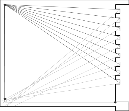
Figure 2: The niches on the right side of the polygon can be guarded using only two scan points.

(a)       $s$ $s$                  (b)   $s$

   (c) $s$          (d) $s$

Figure 3: A number of problems faced by a strategy; the starting point is given by $s$, necessary extensions are drawn dashed. (a) If too many necessary extensions are taken into account, the strategy (left) may end up using a large number of scans, while the optimum takes only one scan (right). (b) When going for next visible corners (dark-gray), the (gray) optimum may not have to leave the base line, causing an arbitrarily bad performance. (c) Going too far beyond a corner may also end up being bad: The optimum needs only a step to the corner and a single scan to see the entire polygon. (d) If the gray line represents the next planed step, the optimum has the opportunity to turn off at some point in the light gray interval.

Even then, a number of problems are faced by an online strategy:

(a) Scanning too often. As opposed to the situation with continuous vision, our strategy needs to avoid too many scans. When simply focusing on edge extensions, we may run into the problem shown in Figure 3(a); this also highlights the problem of not knowing critical extensions before they have been visited. That is, they may not be distinguished from necessary extensions, but scanning on each such one may cause an arbitrarily high competitive ratio.

(b) Where to go next. The robot faces another dilemma when choosing the next scan point: should it walk to the next corner (or the next chosen reference point) itself—or to its perpendicular? Going for the next corner may cause a serious detour, see Figure 3(b).

(c) Missing a scan. As seen in Figure 3(a), it is not a good idea to stop at each corner; on the other hand, when facing a corner in a certain distance and an unknown area behind it, using a predefined point in the unknown interval, e.g., the center or the end, does not allow a bounded competitive ratio, see Figure 3(c).

(d) Missing a turn. Searching for the right distance to place a scan may cause the robot to run beyond an extension, while the optimum may have the opportunity to turn off earlier: e.g., consider the shaded interval in Figure 3 (d). This makes it necessary to consider adjustments and also holds for other situations in which an early turn of the optimum may be possible.

Non-visible regions. Even situations that are trivial for a robot with continuous vision may lead to serious difficulties in the case of discrete vision, as illustrated in Figure 4(left): Without entering the gray area, a watchman with continuous vision is able to see the bold sides completely. A robot with discrete vision is able to see these bold parts of the boundary if only it chooses a scan point under the northernmost part of the boundary. Such an area for which not (yet) all sides which would be completely visible with continuous vision (the bold sides) are visible for a robot with discrete vision, is called a non-visible region (NVR).

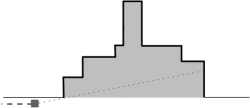
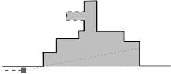
Figure 4: Left: If the dark gray point represent the scan position, a robot with discrete vision cannot see the entire bold sides, resulting in a non-visible region (NVR), shown in gray; an NVR is dealt with by performing a binary search. Scans located in the dotted interval allow for the perception of all sides of the NVR. Right: Within a non-visible region, there may be parts that even a robot with continuous vision may not see completely (dashed), requiring the robot to enter the NVR; such a situation is dealt with by introducing turn adjustments, when the need arises.

All in all, serious adjustments have to be made to establish mathematical structure for exploration with discrete vision; this work is presented in Section 5. Enhanced by several important additional insights and tools (sketched in Sections 6.1 and 6.2), we get our strategy SCANSEARCH, which is presented in Sections 6.3, 6.4, 6.5 , 6.6 and 6.7. The resulting competitive ratios are discussed in Section LABEL:subsec:scansearch.

4 Why the Aspect Ratio Matters

Before developing the details of our $O(\log A)$-competitive strategy for a simple orthogonal polygon with aspect ratio $A$, we illustrate that this is best possible, even for orthoconvex polygons that contain a single niche, given by a staircase to its left and to its right as shown in Figure 5.

Theorem 1.

Let $P$ be a polygon with $n$ edges and aspect ratio $A$. Then no deterministic strategy can achieve a competitive ratio better than $\Omega(\log{A})$, even if $P$ is known in advance to be an orthoconvex polygon.

Proof.

In the beginning, the robot with discrete vision stands at some point with distance $\delta$ to the base line of the niche and small distance $d$ to the perpendicular of one of the corners $a_{0},b_{0}$ (w.l.o.g. $a_{0}$). In an optimal solution, a single scan suffices to see the entire polygon, provided it is taken within the strip shaded in gray. However, the robot does not know the location of this strip, as it depends on reflex vertices of the polygon that are not visible yet. More precisely, let [$a_{0},b_{0}$] be the initial interval. We divide each interval [$a_{i},b_{i}$] into three intervals of equal length; only one of the outermost intervals is open, the other two coincide with the boundary. This defines the new interval [$a_{i+1},b_{i+1}$]; see the middle of Figure 5. Let $x_{i}$ be the position of the robot in the corresponding $i$th interval.

In order to show a lower bound on the competitive strategy we have to construct a scene such that, no matter how the online strategy chooses the next location a certain number of steps cannot be avoided. The scene is constructed by the “adversary”—responding to the behavior of the strategy. Here, choosing the next scan point closer to one boundary, the adversary leaves the other outermost interval open. When choosing the next location in the center of the interval the adversary makes sure with the length of the vertical sides that no information on the layout of the next step is gained.

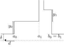
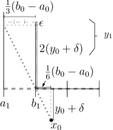
Figure 5: Left: One scan in the gray strip suffices to see the entire niche; middle: definition of $\delta,d,a_{i},b_{i},y_{i}$; right: computing $y_{1}$ to bound the coordinate values.

Choosing $y_{0}=\delta/d(b_{0}-a_{0})+\varepsilon$, $y_{1}=2(y_{0}+\delta)+\varepsilon,\ldots$ the robot cannot see the entire side when located at $x_{i}$. This results in an exponential lower bound for the aspect ratio: the smallest side length in the $i$th step of our construction is $(b_{i}-a_{i})=\left(\frac{1}{3}\right)^{i}(b_{0}-a_{0})$. For the maximum side length we have $2\delta/d3^{i}(b_{0}-a_{0})+T$, $T<f3^{i}(b_{0}-a_{0})$ with some constant $f$. Consequently: $i=1/2\cdot\frac{\log A-\log(2\delta/d+f)}{\log 3}$.

Thus, for any given aspect ratio $A$, a total number of $\Omega(\log A)$ scans cannot be avoided to guarantee full exploration of the niche. Note that the total number of scans can also be described as $\Omega(n)$; however, this lower bound is not purely combinatorial, as it depends on the coding of the input size. ∎

5 Mathematical Foundations

In the following, we will deal with a limited aspect ratio by assuming a minimum edge length of $a$; for simplicity, we assume that the cost of a scan is equal to the time the robots needs for traveling a distance of 1. Hence, we concentrate in the following on $a<1$. Moreover, we still concentrate on orthoconvex polygons.

The correctness of the GREEDY-ONLINE algorithm is based on the propositions of Chin and Ntafos [chinta88], Section 2.3. When considering discrete vision, even the simplest proposition on monotone rectilinear polygons breaks down: Finding an optimum watchman route is not necessarily equivalent to finding a shortest path connecting the top and bottom kernels, as we need to take into account that some scans have to be taken along the way. The cost $t(T)$ of our tour $T$ is a linear combination of the tour length and the number of scan points (in the set S of scan points) used along this route: $t(T)=c\cdot|{\cal S}|+L(T)$. Thus, shortest refers to a tour with lowest cost. In the following, we will develop several modifications for discrete vision of increasing difficulty that lay the foundation for our algorithm SCANSEARCH.

In the following, a visibility path is a path with scans, along which the same area is visible for a robot with discrete vision, as it would be for a human guard with continuous vision. We will proceed by a series of modifications to the results by Chin and Ntafos; modifications are highlighted, and the numbering in parentheses with asterisks refers to that in [chinta88].

Lemma 2 (Lemma 1*).

Finding an optimum watchman route of a robot with discrete vision in a monotone rectilinear polygon is equivalent to finding a shortest visibility path that connects the top and bottom kernels. In case of a polygon that is monotone two both axes the intersection of the kernels is to be considered, cp. Figure 6.

Proof.

We distinguish two cases. If the given polygon is star-shaped, the top and the bottom kernel coincide, and any point in the kernel is an optimum watchman route for a robot.

If the given polygon is not star-shaped, and hence the top and bottom kernel do not coincide, a shortest visibility path between $K_{t}$ and $K_{b}$ is an optimum watchman route:

• First no optimum watchman route of a robot with discrete vision extends above $T$ (the highest bottom edge) or below $B$ (the lowest top edge); in that case, we could find a shorter route as follows.

  If the path to the point above $T$ or below $B$ and the one that leaves that point are the same beyond $T$ or $B$, we move the last scan point to $T$ or $B$ and cut off the end of the route.

  Or, if there is an angle greater than $0$ between the in- and outgoing path, we construct a shorter route by moving the last scan point to $T$ or $B$ (to the point with the shortest distance) and connect the new point with the next scan points.

• Let $S$ be a shortest visibility path from $K_{t}$ (the bottom boundary of the kernel of $P_{t}$, the portion of the polygon that lies above $T$,) to $K_{b}$. Every point in the polygon is visible from some point along $S$: $P_{t}$ and $P_{b}$ are visible from the endpoints of $S$, which lie on $K_{t}$ or $K_{B}$; a point elsewhere in the polygon must be visible because it is visible from the corresponding path of a robot with continuous vision (because of the monotonicity) and the definition of a visibility path.

  Then an optimum watchman route of a robot with discrete vision is formed by following this shortest visibility path and walking backwards (without a scan if possible, i.e., if no shift in direction is needed).

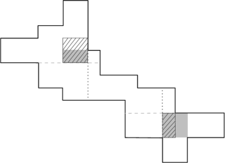
Figure 6: A polygon that is monotone wrt the x- and the y-axis. The top and bottom kernels are shown in light gray and in shaded dark gray.

∎

Just like Chin and Ntafos [chinta88], we now focus on rectilinear simple polygons and adopt their procedure, i.e., we first partition the polygon into uniformly monotone rectilinear polygons and then identify for each of the resulting polygons $R_{i}$ the bottom edges of top kernels ($T_{i}$) and the top edges of bottom kernels ($B_{i}$). First, we identify the essential horizontal edges, and, after applying the method to the polygon after a 90 degrees rotation, the essential vertical edges.

Like in the case of monotone rectilinear polygons, the portions of the polygons that lie outside of the essentials edges will not be visited by any optimum watchman route of the considered robot and are discarded.

Lemma 3 (Lemma 2*).

If $P$ is the original rectilinear simple polygon and $P^{\prime}$ is the new polygon obtained by removing the ”non-essential” portions of the polygon, then no optimum watchman route of a robot with discrete vision will visit any point in $P\setminus P^{\prime}$.

Proof.

If the claim were not true, i.e., there would be an optimum watchman route of a robot with discrete vision visiting a point in $P\setminus P^{\prime}$, this route would cross at least one essential edge. Any point in the section of that edge that is enclosed by the route can see the portion of the polygon that is in $P\setminus P^{\prime}$ so we can make the route shorter, as we would need at least one scan in $P\setminus P^{\prime}$ for the former route as well. Thus, we have a contradiction to the proposition that we have an optimum watchman route. ∎

This allows us to reformulate Lemma 3 of Chin and Ntafos:

Lemma 4 (Lemma 3*).

There is an optimum watchman route of a robot with discrete vision in $P$ that visits the essential edges in the order in which they appear on the boundary of $P^{\prime}$.

Proof.

If an optimum watchman route of a robot with discrete vision does not visit the essential edges in this order, the route will intersect itself.

Then we can restructure this route by deleting this intersection and get a shorter route in which the pre-specified order is followed. If an intersection appears, we must have at least four scan points on the crossing lines. Denote these points by $p_{1},p_{2},p_{3}$ and $p_{4}$, as shown in the left of Figure 7. $p_{1},\ldots,p_{4}$ are located on the paths to or from the essential edges, or on these essential edges. Without loss of generality, the essential edges related to $p_{1},\ldots,p_{4}$ lie in clockwise order on the boundary of $P^{\prime}$.

The following cases can occur:

1. There is no scan point between the $p_{i}$ on the paths. Then Figure 7 shows a route that is shorter by triangle inequality: visit $p_{2}$ directly after $p_{1}$, and $p_{4}$ after $p_{3}$.

   
   

   Figure 7: If there is no scan point between the $p_{i}$, the route may be shortened like this.

2. If a scan point is located on the intersection point, we need to consider two cases:

   1. Either a scan point on one of the lines established in (1.) is sufficient to see all points, then the route in (1.) plus this scan point provides lower cost than the original route.

   2. Or a scan point on one of the lines established in (1.) is not sufficient; in that case we connect two consecutive points by a direct path and use a path via the intersection scan point for the two other points (or if possible a path via a point in shorter distance to two of the $p_{i}$), cp. Figure 8.

      
      

      Figure 8: If a scan point is located on the intersection point, but a scan point on one of the lines established in (1.) is not sufficient, the route may be shortened like this.

3. If one of the $p_{i}$ is the intersection point, we have to consider the route more closely. For that purpose we mention two properties of essential extensions in rectilinear polygons, which were stated by Deng et al. [deng98how].

   Proposition 5 (Proposition 2.2 of Deng et al. [deng98how]).

   • Two distinct essential extensions are either disjoint or perpendicular to each other. (Note that the same essential extension may be the extension of two different sides.)

   • Each essential extension intersects at most two other essential extensions. (If it intersects two other essential extensions, then these two are parallel to each other.)

   The general situation is as shown in Figure 9.

   
   

   Figure 9: The general situation with one of the $p_{i}$ being the intersection point. We have $h\neq j,h\neq k,h\neq l,j\neq k,j\neq l$ and $k\neq l$.

   The paths leading to (or coming from) the essential extensions may have length 0, i.e., the corresponding $p_{i}$ is located on an essential extension.

   • All paths have length $0$:
     Thus, all $p_{i}$ are located on essential extensions. The essential extension on which $p_{j}$ lies must run along $\overline{p_{h}p_{k}}$, because (i) if it cuts $\overline{p_{h}p_{k}}$, $p_{h}$ or $p_{k}$ would lie in $P\setminus P^{\prime}$, and (ii) the essential extension may not be shorter than $\overline{p_{h}p_{k}}$, as running along $\overline{p_{h}p_{j}}$, $\overline{p_{j}p_{k}}$ (independent of direction) would not be possible otherwise. As a result, $\overline{p_{h}p_{k}}$ is completely located on the essential extension. This essential extension is intersected by at most two other essential extensions (see Proposition 5(ii)), which may not intersect between $p_{h}$ and $p_{k}$ (because $p_{i}$ in $P\setminus P^{\prime}$.)

     In the following we distinguish if $p_{1}$ , $p_{4}$, or one of the points $p_{2}$ and $p_{3}$ is the intersection point.

     If $p_{1}$ is the intersection point, not both $p_{2}$ lying before $p_{4}$ in clockwise order and the starting point being located between $p_{4}$ and $p_{1}$, which lie on the same extension, may be true, leading to a contradiction. The same argument holds for $p_{4}$ lying on $\overline{p_{1}p_{3}}$.

     Otherwise, i.e., if $p_{2}$ or $p_{3}$ is the intersection point, these are the only points where the direction is changed, i.e., no “real” intersection appears, and this does not touch the considered order, see Figure 10, but the routes may be shortened.

     

     

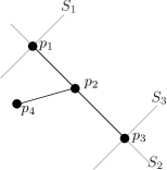
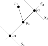
     Figure 10: Left: $p_{2}$ as ”intersection” point, in case of path length = 0. Right: $p_{3}$ as ”intersection” point, in case of path length = 0.

   • At least one path has positive length:
     

     • If $p_{j}=p_{2}$ or $p_{j}=p_{3}$, the route may turn once or thrice.
       When the robot turns only once, $p_{j}$ must be located on an essential extension, as a path to $S_{j}$ would cause another turn. Thus, $p_{h}$ and $p_{k}$ must be located on the same extension (see above), and only a path to $S_{l}$ with positive length is possible. This $p_{j}$ does not influence the requested order, i.e., it is not a “real” intersection point.

       If the robot turns thrice at $p_{j}$ (if the path to $S_{j}$ has positive length), a loop occurs; then the robot may traverse this loop in a way that observes the given order.

     • If $p_{j}=p_{1}$, the route may only use this point thrice.
       If the route does not turn thrice at $p_{1}$, it must start there, as otherwise $\overline{p_{2}p_{4}}$ is an essential extension, and so $p_{3}$ may not lie on a shortest tour, as it would be located in $P\setminus P^{\prime}$.

       If the route turns thrice, the above loop argument holds.

     • $p_{j}=p_{4}$ is analogous to $p_{j}=p_{1}$ (with ends instead of starts).

∎

6 Strategy Aspects

Here we give an overview of the structure of our method; first we give some basic tools (binary search and turn adjustments in 6.1 and 6.2, respectively), followed by high-level case distinctions in the strategy (Sections 6.3, 6.4, 6.5 and 6.6) and a detailed pseudocode for our strategy SCANSEARCH (Section 6.7); for easier reference in checking technical details, we give line numbers. Finally, in Section LABEL:subsec:scansearch we consider the competitive ratio of our strategy.

6.1 Binary Search in the Strategy

As we will often run beyond a point up to which everything is already known, our strategy may force the robot to pass some non-visible regions, which are explored with a binary search strategy. The demand that each edge of the polygon needs to be fully visible from one scan point implies that the robot needs at most $k$ searches ($2k$ if we have NVRs on both sides, see Lemma 6) if the optimum uses $k$ scans. This yields a benchmark for computing the cost of the optimum to determine an upper bound on the competitive ratio.

If we are confronted with one or more non-visible regions lying in an area already passed, the maximum width of the passed area is an upper bound for each possible NVR. Consider a maximum width $w$, and a minimum side length $a$. Then the binary search can be terminated after at most $j^{*}={\log(\frac{w}{a})}$ steps; the total cost is

$$\sum_{j=1}^{\lceil j^{*}\rceil}w\cdot 2^{-j}+\sum_{j=1}^{\lceil j^{*}\rceil}1\leq w-\frac{a}{2}+{\log(\frac{w}{a})}+1$$ (1)

The second sum results from the scans after each move. If we have more than one NVR, we begin with the easternmost, i.e., the one that is closest to the starting point of the move. This may split some NVRs into several NVRs, which are all identified.

Lemma 6.

If the optimum needs $k$ scans in an interval (of width B), the robot needs at most

(i)	$2k$ binary searches if the NVRs may appear on two sides,
(ii)	otherwise $k$ binary searches (with an upper bound given by the above value).

Proof.

If the optimum needs $k$ scans (in the interval of width $B$), we will have $k$ stairs or niches. These will only be visible from the running line if a scan is taken in the integer visibility polygon of the northernmost horizontal edge, as the boundary runs rectilinear, cp. Figure 11. Each of these northernmost horizontal edges lies inside a NVR. These are identified by the robot and each NVR has a width less than or equal to the maximum width. Thus, we need at most a binary search over $mw$ for each of them.

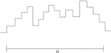
Figure 11: An interval of width B. Scans are required in the integer visibility polygons of the light gray edges.

If the non-visible regions appear on two sides (i), we will need $2k$ binary searches—as a situation like in Figure 12 may occur. That is, with our strategy the robot distinguishes the NVRs, reaches one of the dark gray positions, where one, but not both, of the non-visible regions become visible. Thus, the robot will start another binary search. Consequently, if the optimum takes $k$ scans, the robot will need at most twice as many binary searches.

Figure 12: Worst case for the scan points of the optimum (light gray) and our strategy (dark gray) if the non-visible regions appear on two sides.

∎

6.2 Turn adjustments

In some cases our robot needs to make a turn, but we do not know where the optimum turns (see Figure 3(d)). We handle this uncertainty by considering the maximum corridor possible for turning, move in its center and make an adjustment to the new center whenever a width reduction occurs. Note that we do not make an adjustment when a width increases. When the robot is supposed to make another turn, we adjust to the best possible new position within the corridor. This procedure will be called turn adjustment in the following. The adaptions we apply are described in the proofs of the according lemmas.

Turning in an optimal solution may be the result of a regular turn (Lemma 7), a corridor becoming visible in an NVR, in which case it can be reached by an axis-parallel motion (Lemma 8) or in case the south and eastern boundary are closed (Lemma 9.) In all these cases, we need to make sure that our strategy does not incur too high marginal costs compared to the optimum. We assume that each corridor in the polygon has a minimum corridor width and refer to it as $a_{k}$. With this assumption we know up to which bound we may have to reduce the step length in a binary search.

Lemma 7.

Suppose that in an optimal tour, the optimum turns earlier than we choose to in our strategy. Then the marginal cost of the corresponding turn adjustment remains within a factor of $O(\log A)$ of the optimum.

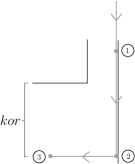
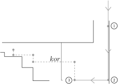
Figure 13: An interval of width kor, in which the optimum could turn earlier. The numbers indicate the order in which the scans are performed.

Proof.

Consider the width $kor$ of the interval in which the optimum may turn earlier, see Figure 13 left. The interval of width kor in which an axis-parallel movement is possible may become narrower because of the boundary (Figure 13 middle). If this keeps the robot from running axis-parallel, the robot runs vertically to the center of the remaining interval, etc. The total cost for these adjustments does not exceed the cost of a binary search in an interval of width kor. If during the search of the non-visible regions we realize that we need to deviate to the south or the north from the horizontal line, i.e., if we find a corridor, we adapt to the best possible position (cost of $kor/2+1$). That is, we adapt to the best height and add a step to the easternmost part of the corridor, if this lies to the south (Figure 13 right).∎

Lemma 8.

Suppose that during the course of the exploration, a corridor is discovered inside of a non-visible region, forcing any optimal solution to make a turn. Then the marginal cost of our strategy remains within a factor of $O(\log A)$ of the optimum.

Proof.

When we discover a corridor, the NVR does not consist of stairs or niches. If the NVR lies south, we look for the first possible eastern corridor, otherwise for the first possible western corridor. The width of the corridor cannot exceed the distance that we covered beyond the extension $E$, and we take this distance as kor. If in the following it is not possible to continue running vertically, the robot runs horizontally to the center of the narrower interval, etc. The costs are estimated by a binary search, and the adjustments are done analogously. ∎

Lemma 9.

Suppose that while a planned axis-parallel move is not possible without a change of direction and the boundary is closed to the south, i.e., no unseen corridor lies to the south, a corridor is discovered that may lie either in the western or the northern area. Then the marginal cost of our strategy remains within a factor of $O(\log A)$ of the optimum.

Proof.

We proceed analogously to the previous argument. Note that the adjustments can happen twice, first in the western, then in the northern area, see Figure 14. Thus, we need two times the upper bound of the binary search in $kor$, $kor/2$ and $1$. ∎

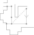
Figure 14: The boundary is closed to the south. Thus, the corridor may either lie to the west or the north. We allow for adjustments in both areas.

6.3 High-Level Decisions within Strategy SCANSEARCH

Just like in the GREEDY-ONLINE strategy by Deng et al., we start with identifying the next extension $E$. Without loss of generality, let the known parts of the boundary run north-south and east-west, and the next extension run north-south, either defined by the bound of the contiguous visible part of the boundary, $f$, or by a sight-blocking corner, $b$. The boundary is in clockwise order completely visible up to the extension. The minimum side length of the polygon $P$ is given and denoted by $a$.

When we want to move we have to

• determine which point we head for and

• decide how to move there.

6.4 Where to Go

To determine the next scan point we first choose a reference point—which, in turn, depends on the next extension in clockwise order.

Case Distinction 1 (Axis-Parallel Movement).

We may

• ] reach the next extension, using an axis-parallel move without a turn or (line 2)

• ] not reach the next extension axis-parallel without a change of direction (line 32).

Our first toehold is the ($L_{2}$-)distance $e$ to $E$—a small distance does not allow for a scan on $E$ and, thus, we will walk beyond it (extension case). $e$ being large enough results in exploring the area up to $E$ (interval case). Here, “large” and “small” depend on the subcases.

Case Distinction 2 (Interval and Extension Case).

• Case [A.]: for $e\geq 2a+1$ (large) we are in interval case (line 3), else in extension case (line 24).

• Case [B.]: for $e\geq a+1$ (large) we are in interval case (line 33), else in extension case (line 90).

Whereas we get a reference point for the extension case, we need to consider other points for the interval case:

Let us first assume to be in case [A.].

Case Distinction 3 (interval case in [A.]).

The next reference point is

• either the perpendicular of the next counterclockwise corner to the shortest path to $E$ ($d_{i}$ being the distance to this point) (line 4 et seqq.) or

• the point on $E$ within distance $e$, if no NVRs appear on the counterclockwise side (line 9).

So, let us now assume to be in case [B.].

Case Distinction 4.

In case an axis-parallel move to $E$ is not possible without a change of direction and $e\geq a+1$, there may be

($\alpha$)	no non-visible regions up to the sight-blocking corner (line 34 et seqq.),
($\beta$)	or non-visible regions up to the sight-blocking corner (line 66 et seqq.).

For ($\alpha$) our point of reference is the sight-blocking corner, let $b_{i}$ be the current distance to this corner.

For ($\beta$) we consider the intersection points of the line between the start position of this case and the sight blocking corner and the extension of the invisible adjacent edge of the next corner on the east-west boundary as well as the extension of the invisible adjacent edge of the next corner on the north-south boundary. Our point of reference is the intersection point with smaller distance, $m_{i}$, to the current position. (Look at Figure LABEL:Beispiel for an example of these cases.)

6.5 Decisions That Affect a Move

So far, we only decided on the reference point for our next move. Now we describe how to determine the point we head for, handle events that occur during movements, and how to perform a move.

In general:

Case Distinction 5 (Planned Distance).

When we face a large distance to the next reference point, we simply go there. When we face a small distance, $r$, to the next reference point, we plan to cover a distance of $2r+1$.

Case Distinction 6 (Crossing a Given Extension).

Let $r$ be the distance to a given reference point. If we plan to cover a distance of $2r+1$ we may

(i)	either not be able to cover the total planned length because of the boundary,
(ii)	or be able to cover the distance of $2r+1$.

Walking a distance of $2r+1$ implies following the axis-parallel line if this is possible ([A.]). Otherwise ([B.]) we end up within a distance of $2r+1$ along the straight connection and go there by walking in an axis-parallel fashion, see Figure 15 (left).

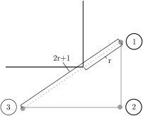
Figure 15: Left: covering a distance of $2r+1$ along the straight connection in moving axis parallel (the numbers indicate the order in which the scans are performed); right: an example for $p_{e},p_{E}$ and $ab_{E}$.

Case Distinction 7 (Line Creation).

Whenever we are in case (ii) of Case 6, we draw an imaginary line parallel to the extension running through the current position. Then we observe whether the entire boundary on the opposite side of this line is visible.

(I)	If this is the case we say that the line creation is positive (lines 21, 31, 52, 63, 78, 88 and 102)
(II)	Otherwise we refer to it as a negative line creation (see for example Figure LABEL:Beispiel) (lines 17, 30, 51,
	62, 77, 87 and 101).

In case of a positive line creation (I), which implies that we do not have to keep on searching in the area behind the line, we move back to $E$ and start searching for a NVR. Otherwise we apply binary search and enter corridors in southern NVRs.

Moreover, for case [B.], we have:

Case Distinction 8 (Covering the Total Planned Length Is Not Possible).

If we meet the preconditions of Case 6(i) and an axis-parallel move to $E$ is not possible without a change of direction, the boundary is

(a)	either not closed south of the path (lines 44, 59, 74, 84 and 98)
(b)	or closed south of the path (lines 47, 60, 75, 85 and 99).

6.6 How to Move

The further movements and actions depend on the distances in cases [A.] and [B.]:
[A.]:

• If the distance to the next reference point is big enough, we cover this distance.

• Otherwise we walk beyond this point (Case Distinction 6).
  Case 6(i) results in moving as far as possible, moving back to $E$, applying binary search for NVRs (up to $E$ on one side, beyond $E$ on both sides) and using a corridor whenever we find one (with turn adjustments).
  Case 6(ii) is the precondition of Case Distinction 7.

[B.]:
In the extension case without the possibility to reach $E$ axis-parallel without a change of direction (l 90 et seqq.) we refer to the point in which the axis-parallel move to $E$ changes the direction as $p_{e}$. $p_{E}$ is the next corner on the boundary in clockwise order, and $ab_{E}$ is the distance from the current starting point to $p_{E}$, see Figure 15 (right). With $ab_{E}$ we have again the critical distance.

Case Distinction 9.

If we face the extension case without the possibility to reach $E$ axis-parallel without a change of direction, we distinguish two possible motions:

• If $ab_{E}$ is large ($ab_{E}>2a+3$) we cover a distance of $2e+1$ along the straight connection in moving axis-parallel. (The distance to $p_{E}$ allows us to do so on the first axis-parallel line.) This results again in the basic case distinctions 6, 7 and 8.

• For $ab_{E}\leq 2a+3$ (small) we move to $E$ via $p_{E}$ and—if necessary—apply binary search and make turn adjustments.

The interval case without the possibility of reaching $E$ axis-parallel without a change of direction (line 33 et seqq.) requires some more case analysis.

($\alpha$): Let $b_{i}$ be the distance to the sight-blocking corner, which is our point of reference.

• Thus, if $b_{i}$ is larger than $2a+1$, we walk to the sight-blocking corner. As always when axis-parallel moves without a turn are not possible, we cover this distance in an axis-parallel fashion (line 35), cp. Figure LABEL:StrFig (left).
  

• Case Distinction 10.

  If $b_{i}<2a+1$ holds:

  • Either we may be able to cover a distance of $2b_{i}+1$ and run beyond $E$ on the second axis-parallel line (after the change of direction), which results in the case distinction (and movements) of Case distinctions 6, 7 and 8 (line 41 et seqq.), cp. Figure LABEL:StrFig (middl)e.

  • Or the point where we would have to change our direction ($p_{cor}$) may not lie inside the polygon (line 53). So we walk to $p_{E}$ (see Figure 15 (right) for the definition and Figure LABEL:StrFig (right) for the actual move) and then axis-parallel to the straight connection. In doing so we

    $\bullet$	either do not run beyond $E$ (line 54)
    $\bullet$	or would run beyond $E$ (line 57), resulting again in the case distinctions 6, 7 and 8.

  • Otherwise turn adjustments are used (line 64).

($\beta$): With NVRs appearing up to the sight-blocking corner ($\beta$) we consider other points of reference, but the structure is the same as in ($\alpha$). The critical distance $m_{i}$ is the shortest distance to the intersection point of the straight connection to the sight-blocking corner and the extension of one side of an NVR. Moreover, the point that is equivalent to $p_{cor}$ is called $p_{m}$ (line 66 et seqq.).

For $a>1$ we use a similar strategy (line 103 et seqq.). Because scans are taken whenever a distance of $a$ is covered, NVRs are explored while passing and corridors are identified immediately.

While exploring the polygon, we make sure that in clockwise order all parts of the polygon are visible after having been passed, i.e., we make sure that we see everything a watchman with continuous vision would see when walking along the basic path. Areas that are not visible define an extension in the remaining part of the algorithm, and we always use the next clockwise corridor. Moreover, we return to the starting point as soon as we have seen all sides of the boundary.

6.7 The strategy SCANSEARCH

Input: A starting position inside an unknown rectilinear polygon $P$, its minimum side length $a$, its minimum corridor width $a_{k}$.

Output: A route along which the whole polygon becomes visible for a robot with discrete vision, such that each edge is fully visible from some scan point.

We identify the next extension in analogy to the GREEDY-ONLINE algorithm of Deng et al. [deng98how], i.e., we update $C,f$ and $M$ whenever changes occur.

If $f$ is a reflex corner, let $E=Ext(F(f))$. Otherwise let $b$ be the blocking corner when $f^{-}$ was in view, and let $E=Ext(B(b))$.

If it is possible to move axis-parallel to $E$ without a change of direction, let $e$ be the axis-parallel distance to $E$; otherwise, let $e$ be the shortest distance to $E$ without a change of direction.

$a\leq 1$:   [A.] An axis-parallel move to $E$ is possible without a turn:   [*] $e\geq 2a+1$: interval case   [1.] If $d_{i}>2a+1$, move to the perpendicular of the corner.

  [2.] If $d_{i}\leq 2a+1$: ;

if $d_{i}>a$: cover a distance of $2d_{i}+1$;

if $d_{i}\leq a$: cover a distance of $2a+1$;

apply binary search if necessary, i.e., if non-visible regions appear.

  [3.] If no corner appears on the counterclockwise side, move directly to $E$.

If we run beyond $E$ with a step of length $2d_{i}+1$/$2a+1$:   (i) If we do not cover the total distance, because of the boundary:

Run as far as possible, go back to $E$, move back in steps of length 1, apply binary search for NVRs (on the counterclockwise side till $E$, on both sides beyond $E$); if a corridor is identified, use it and make turn adjustments. (If a critical extension is found, search only on the opposite side.)

  (ii) If we may cover the total distance of $2d_{i}+1$/$2a+1$:   (I) negative line creation:

Apply binary search; if a corridor is discovered inside an NVR, use it and make turn adjustments. (Because the line creation is negative, only corridors in southern non-visible regions are used.)

  (II) positive line creation:

Go back to $E$, move back in steps of length 1, apply binary search and search for a corridor and the critical extension, making turn adjustments.

  [*] $e<2a+1$: extension case

Consider running a distance of $2e+1$.   (i) If it is not possible to run a distance of $2e+1$: Run as far as possible, go back to $E$, move back in steps of length 1, apply binary search for NVRs and, if a corridor is identified, use it and make turn adjustments.

  (ii) If we may cover the total distance of $2e+1$:   (I) negative line creation.

  (II) positive line creation.

Algorithm 1 The strategy SCANSEARCH

31

31

31

31

31

31

31

31

31

31

31

31

31

31

31

31

31

31

31

31

31

31

31

31

31

31

31

31

31

31

31

  [B.] An axis-parallel move to $E$ is not possible without a change of direction:   [*] $e\geq a+1$: interval case

($\alpha$) No non-visible region up to the sight-blocking corner   [1.] If $b_{i}>2a+1$, move axis-parallel to the corner, see Figure LABEL:StrFig, left.

  [2.] If $b_{i}\leq 2a+1$, cover a distance of $2b_{i}+1$ along the straight connection in moving axis-parallel and visiting $p_{cor}$, see Figure LABEL:StrFig, middle. If necessary, apply binary search. Apply the binary search on the first axis-parallel line before leaving $p_{cor}$ in a right angle to this line and apply the binary search on the second axis-parallel afterwards.

Now distinguish the following.   ($\mathcal{A}$) If we run beyond $E$ (on the second axis-parallel line):   (i) If it is not possible to cover the total planned length, let $\alpha_{i}$ be the distance to this boundary along the straight connection, and   (a) if the boundary is not closed south of the path, i.e., the clockwise exploration of the polygon continues south of the second axis-parallel line, then move as far as possible, apply binary search on both axis-parallel lines and make turn adjustments.

  (b) if the boundary is closed south of the path, then move as far as possible, apply binary search on both axis-parallel lines and apply turn adjustments, if necessary twice, as we are in the last case of the turn adjustments.

  (ii) If it is possible to cover the total planned length, we distinguish:   (I) negative line creation.

  (II) positive line creation.

  ($\mathcal{B}$) If it is not possible to run via $p_{cor}$ (as the boundary blocks us from doing so) and   $\bullet$ if we do not run beyond $E$ in doing so: Run to $p_{E}$ (see Figure LABEL:StrFig, right) and then axis-parallel to the straight connection. If necessary, apply binary search and make turn adjustments.

  $\bullet$ if we would run beyond $E$:   (i) If it is not possible to cover the total planned length:   (a) If the boundary is not closed south of the path.

  (b) If the boundary is closed south of the path.

  (ii) If it is possible to cover the total planned length, we distinguish:   (I) negative line creation.

  (II) positive line creation.

  ($\mathcal{C}$) neither ($\mathcal{A}$) nor ($\mathcal{B}$) is true, make turn adjustments (like in the first case of the turn adjustments).

65

65

65

65

65

65

65

65

65

65

65

65

65

65

65

65

65

65

65

65

65

65

65

65

65

65

65

65

65

65

65

65

65

65

    ($\beta$) Along the boundary up to the sight-blocking corner occur non-visible regions   [1.] If $m_{i}>2a+1$, cover a distance of $m_{i}$ along the straight connection in moving axis-parallel and visiting $p_{m}$.

  [2.] If $m_{i}\leq 2a+1$, cover a distance of $2m_{i}+1$ along the straight connection in moving axis-parallel and apply binary search if necessary.

In (2.) several cases may occur:   ($\mathcal{A}$) If we run beyond $E$ (on the second axis-parallel line):   (i) If it is not possible to cover the total planned length:   (a) If the boundary is not closed south of the path.

  (b) If the boundary is closed south of the path.

  (ii) If it is possible to cover the total planned length, we distinguish:   (I) negative line creation.

  (II) positive line creation.

  ($\mathcal{B}$) If it is not possible to run via $p_{m}$ (as the boundary hinders us to do so) and   $\bullet$ if we will not run beyond $E$ in doing so: Run to $p_{E}$ and then axis-parallel to the straight connection. If necessary apply binary search and make turn adjustments.

  $\bullet$ if we run beyond $E$:   (i) If it is not possible to cover the total planned length:   (a) If the boundary is not closed south of the path.

  (b) If the boundary is closed south of the path.

  (ii) If it is possible to cover the total planned length, we distinguish:   (I) negative line creation.

  (II) positive line creation.