The One-Loop Five-Graviton Amplitude and the Effective Action

Abstract:

We consider the one-loop five-graviton amplitude in type II string theory calculated in the light-cone gauge. Although it is not possible explicitly to evaluate the integrals over the positions of the vertex operators, a low-energy expansion can be obtained, which can then be used to infer terms in the low-energy effective action. After subtracting diagrams due to known $D^{2n}R^{4}$ terms, we show the absence of one-loop $R^{5}$ and $D^{2}R^{5}$ terms and determine the exact structure of the one-loop $D^{4}R^{5}$ terms where, interestingly, the coefficient in front of the $D^{4}R^{5}$ terms is identical to the coefficient in front of the $D^{6}R^{4}$ term. Finally, we show that, up to $D^{6}R^{4}\sim D^{4}R^{5}$, the $\epsilon_{10}$ terms package together with the $t_{8}$ terms in the usual combination $(t_{8}t_{8}\pm\frac{1}{8}\epsilon_{10}\epsilon_{10})$.

1 Introduction

At low energies, the way in which string theory differs from conventional field theory is best encoded by the low-energy effective action which, beyond lowest order, gives important stringy corrections to supergravity. These corrections are relevant for a whole host of physics. They modify Calabi-Yau compactifications to four dimensions by, for example, correcting the metric for the universal hypermultiplet [1, 2]. They are also important for testing AdS/CFT beyond leading order, where they give rise to $1/N$ and $1/\lambda$ effects in the field theory [3, 4]. Further, if string theory is to provide the microscopic description of black holes and black branes then higher order corrections must play a crucial rôle [5, 6, 7]. Stringy corrections are also relevant for understanding the dualities between string theories and eleven-dimensional supergravity [8, 9], and perhaps even for understanding M-theory.

The meaning of the effective action in string theory is often not well explained. It bears similarities to both the Wilsonian and 1PI actions, but is identical to neither. The classical string field theory action is a functional of both massless and massive fields, $S(\phi_{0},\phi_{h})$. For low-energy physics only the massless modes are explicitly relevant and so it makes sense to perform the path integral over the massive modes,

$$e^{iS_{\rm eff}(\phi_{0})}=\int\mathcal{D}\phi_{h}e^{iS(\phi_{0},\phi_{h})}.$$ (1)

This differs from the usual Wilsonian effective action since the path integral over massless modes with high-momentum has not been performed. If amplitudes are calculated from $S_{\rm eff}(\phi_{0})$ it is still necessary to consider loops of massless particles. Generically such an action will be non-local and its utility derives from a low-energy expansion, which is equivalent to a derivative expansion.

Ideally we would be able to quantize $S(\phi_{0},\phi_{h})$ and find its corresponding 1PI action, $\Gamma[\phi_{\rm cl}]$. This would be some functional of all possible fields in string theory, including massive fields and D-brane fields. Even in the absence of this, we can still construct the one-particle irreducible action for $S_{\rm eff}(\phi_{0})$, which we call $S_{\rm eff,1PI}(\phi_{0})$. This is presumably equivalent to $\Gamma[\phi_{\rm cl}]$ with the massive fields set to zero. The full string field theory 1PI action $\Gamma[\phi_{\rm cl}]$ could in principle be used to find correlation functions about any background of string theory. Since $S_{\rm eff,1PI}(\phi_{0})$ only involves fields which are massless in Minkowski space, it is unclear whether it can be used in this way. However, it may well still give amplitudes around backgrounds which share the same massless spectrum as Minkowski space. For example, it is often believed that $S_{\rm eff,1PI}(\phi_{0})$ expanded in small fluctuations around $AdS_{5}\times S^{5}$ gives correct $AdS_{5}\times S^{5}$ amplitudes for massless states. However, it is not known whether correct results would be obtained about backgrounds containing other massless fields, such as various conifolds where D-branes become massless by wrapping vanishing cycles.

Amplitudes derived from $S_{\rm eff,1PI}(\phi_{0})$ should only include tree diagrams. In this sense $S_{\rm eff,1PI}(\phi_{0})$ resembles the usual 1PI action. However, since massive fields are ignored and since its status about backgrounds other than Minkowski is unclear, it is perhaps not the full quantum effective action. The term effective action in this paper, and in most of the string theory literature, refers to $S_{\rm eff,1PI}(\phi_{0})$, which we define as the action whose tree diagrams generate string theory amplitudes in Minkowski space at all orders in the string coupling. However, it should be noted that non-local terms due to thresholds will not be calculated. In principle, this implies no loss of information since such terms can be reinstated using unitarity and the tree-level effective action, but without them the effective action cannot really be claimed to be the full 1PI action.

There are at least three common ways to determine the effective action. Firstly, one can calculate the world-sheet $\beta$-functions. Since scale invariance at the quantum level requires all $\beta$-functions to vanish, these lead to equations of motion and an action for the background fields. Secondly, one can try to use various symmetries, for example supersymmetry or $SL(2,\mathbb{Z})$ invariance, to extend known terms to more complete expressions. Finally, one can directly calculate string scattering amplitudes and deduce the on-shell effective action which reproduces them. It is this last method which is used here.

We calculate amplitudes using the light-cone gauge Green-Schwarz formalism. The greatest problem with this formalism is that a convenient representation for the vertex operators is only available when all external states satisfy $k^{+}=0$. As a consequence, not all terms in the amplitude, and so in the effective action, can be discovered. For example, this formalism cannot be used to determine whether the effective action contains the term

$${\epsilon_{10\,m}}^{a_{1}\cdots a_{9}}{\epsilon_{10}}^{mb_{1}\cdots b_{9}}R_{a_{1}a_{2}b_{1}b_{2}}R_{a_{3}a_{4}b_{3}b_{4}}R_{a_{5}a_{6}b_{5}b_{6}}R_{a_{7}a_{8}b_{7}e}{{R_{a_{9}}}^{e}}{}_{b_{8}b_{9}},$$ (2)

with only one contraction between the $\epsilon_{10}$ tensors. Similarly, the $B\wedge t_{8}R^{4}$ term found in type IIA [11] cannot be determined. The only terms that will be missed in this paper are those with a single $\epsilon_{10}$ tensor and those involving fewer than two contractions between a pair of $\epsilon_{10}$ tensors. Terms like the famous $\epsilon_{10}\epsilon_{10}R^{4}$, which has two contractions between the $\epsilon_{10}$’s, will still be visible.

For both type II theories, the first correction to the Einstein-Hilbert term is the tree-level $\alpha^{\prime 3}R^{4}$ term which is given in string frame by

$$\alpha^{\prime 3}\int d^{10}x\sqrt{-g}\,e^{-2\phi}\,t_{8}^{a_{1}b_{1}\cdots a_{4}b_{4}}t_{8}^{c_{1}d_{1}\cdots c_{4}d_{4}}R_{a_{1}b_{1}c_{1}d_{1}}R_{a_{2}b_{2}c_{2}d_{2}}R_{a_{3}b_{3}c_{3}d_{3}}R_{a_{4}b_{4}c_{4}d_{4}},$$ (3)

where $t_{8}$ is defined in the next section. There is a similar term at the next order in string coupling with $e^{-2\phi}$ replaced by $1$ and with a different coefficient. If terms involving $\epsilon_{10}$ tensors are also considered then (3) is extended by replacing $t_{8}t_{8}$ by $(t_{8}t_{8}\pm\frac{1}{8}\epsilon_{10}\epsilon_{10})$. These terms are supplemented by a whole host of terms involving fields other than the graviton, such as $R^{n}(DH)^{4-n}$ [12], $R^{2}(DF)^{2}$ [13] and $\Lambda^{16}$ [14], where $H$ and $F$ are the $NS\otimes NS$ and $R\otimes R$ three-form field strengths respectively and $\Lambda$ is the dilatino.

In the absence of an off-shell definition of string field theory, the effective action is only fixed up to field redefinitions. As a consequence, any terms which vanish when evaluated on the lower-order equations of motion can be removed. In particular, this implies that Ricci tensors and Ricci scalars can always be eliminated. So, at order $\alpha^{\prime}$ for example, a field redefinition can be used to remove $R_{ab}R^{ab}$ and $R^{2}$, leaving just $R_{abcd}R^{abcd}$. The fact that the Riemann-squared term also vanishes in type II is a non-trivial consequence of this particular theory. Similarly, since the Riemann and Weyl tensors only differ by terms involving $R_{ab}$ and $R$, the $t_{8}t_{8}R^{4}$ term can equivalently be rewritten as $t_{8}t_{8}C^{4}$.

At higher orders in $\alpha^{\prime}$ far less is known. Certain $D^{2n}R^{4}$ terms have been found from the expansion of the four-graviton amplitude, for example $\alpha^{\prime 5}t_{8}t_{8}D^{4}R^{4}$ and $\alpha^{\prime 6}t_{8}t_{8}D^{6}R^{4}$, but little is known about terms involving more Riemann tensors or other fields. At $\alpha^{\prime 4}$ and beyond it is possible for $R^{5}$ and $D^{2n}R^{5}$ terms to appear. The purpose of this paper is to determine such terms at one-loop up to and including $\alpha^{\prime 6}D^{4}R^{5}$. To do so we calculate the five-graviton amplitude on a toroidal world-sheet and determine its expansion in powers of $\alpha^{\prime}$. Before new terms can be constructed, it is important to subtract contributions from known $D^{2n}R^{4}$ terms. After doing so, the remaining terms (if any) can be covariantised to give new $R^{5}$ and $D^{2n}R^{5}$ terms. The plan of this paper is as follows. Section 2 reviews the case of four-gravitons – the amplitude, its expansion and the effective action – which leads to the well-known $D^{2n}R^{4}$ terms. The calculation of the five-graviton amplitude is reviewed and simplified in section 3 before determining its low-energy expansion in section 4 using an extension of the four-graviton techniques. Section 5 calculates all the relevant field theory diagrams arising from the known $D^{2n}R^{4}$ terms. After subtracting these from the expanded amplitude, the presence of $R^{5}$ and $D^{2n}R^{5}$ terms are determined. The extension of this analysis to include $\epsilon_{10}\epsilon_{10}$ terms is contained in section 6, where the equivalent of $(t_{8}t_{8}\pm\frac{1}{8}\epsilon_{10}\epsilon_{10})R^{4}$ at higher orders in $\alpha^{\prime}$ is studied. Appendix A contains various identities linking the three tensors, $t_{10}$, $\bar{t}_{10}$ and $t_{8}$, which arise when calculating the amplitude. Throughout we will use a metric with signature $\{-,+,+,+,\ldots\}$ and will often set $2\alpha^{\prime}=1$.

2 The Effective Action from the Four-Graviton Amplitude

Before we embark on studying the type II five-graviton amplitude, we review the equivalent results for the four-graviton amplitude. Let the four particles have polarisation tensors $h^{r}_{a_{r}b_{r}}$ and momenta $k^{r}_{a_{r}}$, where $r=1,\ldots,4$ and $a,b=0,\ldots,9$. There are three Mandelstam variables defined by

$$s=-(k_{1}+k_{2})^{2},\qquad t=-(k_{1}+k_{3})^{2},\qquad u=-(k_{1}+k_{4})^{2},$$ (4)

which are related by $s+t+u=0$. The one-loop amplitude is well-known to be given by [15]

$$A_{4h}=\hat{K}\int_{\cal F}\!\frac{d^{2}\tau}{({\rm Im}\,\tau)^{5}}\int_{\cal T}\prod_{r=1}^{3}d^{2}v_{r}\prod_{r<s}(\chi_{rs})^{\frac{1}{2}k_{r}\cdot k_{s}},$$ (5)

where

$$\hat{K}=t_{8}^{a_{1}b_{1}\cdots a_{4}b_{4}}t_{8}^{c_{1}d_{1}\cdots c_{4}d_{4}}k^{1}_{a_{1}}k^{1}_{c_{1}}h^{1}_{b_{1}d_{1}}k^{2}_{a_{2}}k^{2}_{c_{2}}h^{2}_{b_{2}d_{2}}k^{3}_{a_{3}}k^{3}_{c_{3}}h^{3}_{b_{3}d_{3}}k^{4}_{a_{4}}k^{4}_{c_{4}}h^{4}_{b_{4}d_{4}},$$ (6)

and where we have set $2\alpha^{\prime}=1$. Here $v_{r}$ are the positions of the four vertex operators on the world-sheet torus and are integrated over the rectangular region $-\frac{1}{2}<{\rm Re}\,v\leq\frac{1}{2},-\frac{1}{2}{\rm Im}\,\tau<{\rm Im}\,v\leq\frac{1}{2}{\rm Im}\,\tau$, which we denote by ${\cal T}$. The variable $\tau$ parameterizes the modulus of the torus and so should be integrated over a fundamental domain of $SL(2,\mathbb{Z})$; to facilitate the low-energy expansion, it is convenient to use the fundamental domain given in figure 1, which we denote by ${\cal F}$. The function $\chi_{rs}\equiv\chi(v_{rs},\tau)$, $v_{rs}\equiv v_{r}-v_{s}$, is a non-singular doubly periodic function of $v$ and $\bar{v}$ which is explicitly given by

$$\chi(v,\tau)=2\pi\exp\left(-\frac{\pi({\rm Im}\,v)^{2}}{{\rm Im}\,\tau}\right)\left|\frac{\theta_{1}(v,\tau)}{\theta_{1}^{\prime}(0,\tau)}\right|,$$ (7)

where $\theta_{1}(v,\tau)$ is the usual Jacobi theta function given, for example, in [16].

Figure 1: One of the fundamental domains of $SL(2,\mathbb{Z})$.

The $t_{8}$ tensor is an eight-component tensor originating from the trace over eight fermionic zero modes and can be written explicitly as a sum of an eight-component $\epsilon_{8}$ tensor and sixty $\delta\delta\delta\delta$ tensors [16],

$$t_{8}^{a_{1}b_{1}a_{2}b_{2}a_{3}b_{3}a_{4}b_{4}}= \pm{\textstyle\frac{1}{2}}\epsilon_{8}^{a_{1}b_{1}a_{2}b_{2}a_{3}b_{3}a_{4}b_{4}}$$

$$-{\textstyle\frac{1}{2}}\big{(}(\delta^{a_{1}a_{2}}\delta^{b_{1}b_{2}}-\delta^{a_{1}b_{2}}\delta^{a_{2}b_{1}})(\delta^{a_{3}a_{4}}\delta^{b_{3}b_{4}}-\delta^{a_{3}b_{4}}\delta^{a_{4}b_{3}})$$

$$\qquad+(1,2,3,4)\to(1,3,2,4)$$

$$\qquad+(1,2,3,4)\to(1,4,2,3)\big{)}$$

$$+{\textstyle\frac{1}{2}}\big{(}\delta^{a_{1}a_{2}}\delta^{b_{1}b_{3}}\delta^{b_{2}b_{4}}\delta^{a_{3}a_{4}}+\delta^{a_{1}a_{2}}\delta^{b_{1}b_{4}}\delta^{b_{2}b_{3}}\delta^{a_{3}a_{4}}+\delta^{a_{1}a_{3}}\delta^{b_{1}b_{4}}\delta^{b_{2}b_{3}}\delta^{a_{2}a_{4}}$$

$$\qquad+\mbox{45 other terms determined by antisymmetry}\big{)},$$ (8)

with the $\pm$ sign depending on the $SO(8)$ chirality. It has symmetries not dissimilar to the Riemann tensor: it is antisymmetric under interchange of any pair of indices $a_{r}$ with $b_{r}$, and is symmetric under interchanging the pair $(a_{r},b_{r})$ with the pair $(a_{s},b_{s})$. It is worth noting that $t_{8}$ is often defined without the $\epsilon_{8}$ tensor, especially in effective actions, and we will clarify this issue later. However, for the four-graviton amplitude this difference is unimportant since all terms involving an $\epsilon$ vanish due to momentum conservation.

As with all amplitudes, $A_{4h}$ is not necessarily finite for all values of the external momenta. Poles occur when the momenta are such that an on-shell intermediate particle can be produced. On the world-sheet, this is interpreted as two states approaching each other and developing a long tube separating them from the other states. By expanding around $v_{rs}=0$ for some fixed $r$, $s$, and using $\chi(v,\tau)\sim 2\pi|v|$ for small $v$, it is easy to show that the lightest pole goes like $\frac{1}{\alpha^{\prime}k_{r}\cdot k_{s}+2}$ and so is massive. The absence of massless poles is consistent with the vanishing of the one-loop amplitude for three gravitons. There are also threshold branch cuts when the external momenta are sufficiently large to produce two or more physical states which circulate around the loop. These originate from the region where the torus degenerates to a thin wire, i.e.  ${\rm Im}\,\tau\to\infty$, which causes $\chi(v,\tau)$ to diverge.

However, it is not possible to see all these poles and thresholds from the integral representation of the amplitude given in (5). In fact, the integral representation only converges at the single point $s=t=u=0$. The resolution is to split the integration over the $v_{r}$ into six regions depending on the ordering of the ${\rm Im}\,v_{r}$. For example, for the region $0\leq{\rm Im}\,v_{1}\leq{\rm Im}\,v_{2}\leq{\rm Im}\,v_{3}\leq{\rm Im}\,\tau$, we eliminate $t$ and consider the amplitude as a function of complex $s$ and $u$. Then it can be shown that avoiding singularities when $v_{rs}\to 0$ requires $s<8$, $u<8$ and $s+u>-8$. Similarly, avoiding the singularity as ${\rm Im}\,\tau\to\infty$ requires $s\leq 0$ and $u\leq 0$. So, taken together, this region of the amplitude only converges in the infinite strip $s\leq 0$, $u\leq 0$ and $s+u>-8$. It is then possible to analytically continue this strip to the entire complex plane. The real physical amplitude should be understood as the sum of the continuation of all six regions. Only after continuing can the amplitude be shown to contain all the correct massive poles, massive double poles and thresholds required by unitarity [17, 18, 19].

2.1 Low-energy Expansion of the Amplitude

Before determining the low-energy effective action, it is necessary to expand the amplitude in powers of $\alpha^{\prime}s$, $\alpha^{\prime}t$ and $\alpha^{\prime}u$. In particular, we need to expand

$$I=\int_{\cal F}\!\frac{d^{2}\tau}{({\rm Im}\,\tau)^{5}}\int_{\cal T}\prod_{r=1}^{3}d^{2}v_{r}\prod_{r<s}(\chi_{rs})^{\frac{1}{2}k_{r}\cdot k_{s}}.$$ (9)

Massive poles in $A_{4h}$ will not be visible at low energies, but threshold corrections will still be present as branch cuts. Due to the symmetry of $I$ in $s$, $t$ and $u$, the expansion will have the form,

$$I=a+\frac{\alpha^{\prime}}{4}I_{\rm nonan}(s,t,u)+b\frac{\alpha^{\prime 2}}{16}(s^{2}+t^{2}+u^{2})+c\frac{\alpha^{\prime 3}}{64}(s^{3}+t^{3}+u^{3})+\cdots,$$ (10)

where $a$, $b$ and $c$ are constants that we wish to determine. $I_{\rm nonan}$ is the first non-analytic term due to thresholds and contains terms of the form $s\ln s$. Using unitarity, it can be seen to arise from two four-graviton tree-level amplitudes connected by a pair of on-shell gravitons. The lack of other non-analytic terms before order $\alpha^{\prime 4}$ is related to the fact that, for type II theories, the first correction to the effective action is at order $\alpha^{\prime 3}$ relative to the Einstein-Hilbert term. There is no analytic term at order $\alpha^{\prime}$ since $s+t+u$ vanishes. Despite being symmetric in $s$, $t$, $u$, there is no need for an $st+su+tu$ term at order $\alpha^{\prime 2}$ since this is proportional to $s^{2}+t^{2}+u^{2}$. Similarly, at order $\alpha^{\prime 3}$, the other possible symmetric expressions, i.e.  $st^{2}+su^{2}+\ldots$ and $stu$, are both proportional to $s^{3}+t^{3}+u^{3}$. It is worth noting that this property does not continue indefinitely: eventually terms other than $s^{n}+t^{n}+u^{n}$ will appear. Since $s$, $t$ and $u$ are not independent it is useful to eliminate $u$ leaving,

$$I-I_{\rm nonan}=a+b\frac{\alpha^{\prime 2}}{8}(s^{2}+t^{2}+st)-c\frac{3\alpha^{\prime 3}}{64}(s^{2}t+st^{2})+\cdots.$$ (11)

The constants $a$, $b$ and $c$ were first determined in [20], which we review here since similar techniques will be required to expand the five-graviton amplitude. By differentiating (11) and taking the limit $s,t\to 0$, we need to consider expressions such as

$$c=-\frac{2^{8}}{3(2\alpha^{\prime})^{3}}\lim_{s,t\to 0}\partial_{s}^{2}\partial_{t}(I-I_{\rm nonan}),$$ (12)

where

$$\lim_{s,t\to 0}\partial_{s}^{m}\partial_{t}^{n}I =\left(-\frac{1}{4}\right)^{m+n}\int_{\cal F}\!\frac{d^{2}\tau}{({\rm Im}\,\tau)^{5}}\int_{\cal T}\prod_{r=1}^{3}d^{2}v_{r}\,(\ln\chi_{12}+\ln\chi_{34}-\ln\chi_{14}-\ln\chi_{23})^{m}$$

$$\qquad\quad\times(\ln\chi_{13}+\ln\chi_{24}-\ln\chi_{14}-\ln\chi_{23})^{n}.$$ (13)

The non-analytic parts originate from the region of moduli space where ${\rm Im}\,\tau\to\infty$, interpreted as the torus degenerating into a thin wire. To remove them, the $\tau$-integral over the fundamental domain is split into two parts: a part with ${\rm Im}\,\tau\leq L$, for large $L$, which will contain the required constant term and an $L$-dependent term; and a part with ${\rm Im}\,\tau>L$, which will contain the non-analytic piece and an $L$-dependent term. Since the overall integral cannot depend on $L$, the $L$-dependent terms must cancel between the two regions. The constant piece can be found by restricting to the first region and ignoring $L$-dependent pieces. To perform the $v_{r}$-integrals, it is convenient to represent $\ln\chi$ as a Fourier series,

$$\ln\chi(v,\tau) =-\frac{1}{2\pi}\sum_{(m,n)\neq(0,0)}\frac{{\rm Im}\,\tau}{|m\tau+n|^{2}}\exp\left[2\pi im\left({\rm Re}\,v-\frac{{\rm Re}\,\tau}{{\rm Im}\,\tau}{\rm Im}\,v\right)-2\pi in\,\frac{{\rm Im}\,v}{{\rm Im}\,\tau}\right]$$

$$\qquad\quad-\left|\ln\sqrt{2\pi}\eta(\tau)\right|^{2},$$ (14)

where $\eta(\tau)$ is the Dedekind eta-function. Since $\ln\chi$ always occurs in positive and negative pairs in (2.1), the zero mode part containing $\eta(\tau)$ cancels out and can be ignored.

Since there are no non-analytic terms at lowest order, the calculation of $a$ can be performed by integrating $\tau$ over the entire fundamental domain,

$$a=\lim_{s,t\to 0}I=\int_{\cal F}\!\frac{d^{2}\tau}{({\rm Im}\,\tau)^{5}}\int_{\cal T}\prod_{r=1}^{3}d^{2}v_{r}=\int_{\cal F}\!\frac{d^{2}\tau}{({\rm Im}\,\tau)^{2}}=\frac{\pi}{3}.$$ (15)

2.1.1 Calculation of $b$

Setting $2\alpha^{\prime}=1$ and twice differentiating (11) with respect to $s$, the coefficient $b$ is given by

$$b=\int_{\cal F}\!\frac{d^{2}\tau}{({\rm Im}\,\tau)^{5}}\int_{\cal T}\prod_{r=1}^{3}d^{2}v_{r}\,(\ln\chi_{12}+\ln\chi_{34}-\ln\chi_{14}-\ln\chi_{23})^{2}\,\bigg{|}_{\rm const},$$ (16)

where $|_{\rm const}$ refers to the constant ($L$-independent) piece of the restricted $\tau$-integral, i.e.  the integral over only the ${\rm Im}\,\tau\leq L$ region. Expanding the brackets yields two type of terms: cross-terms and square-terms. After redefinitions of the $v_{r}$, the $v_{r}$-integrals for all six of the cross-terms are equivalent to $\left(\int_{\cal T}d^{2}v\,\ln\chi\right)^{2}\left(\int_{\cal T}d^{2}v\right)$, which vanishes since the integral over a single $\ln\chi(v,\tau)$ is zero (recall that the zero mode part of $\ln\chi$ has been removed). The four square-terms are all equivalent to

$$\left(\int_{\cal T}d^{2}v\,(\ln\chi)^{2}\right)\left(\int_{\cal T}d^{2}v\right)^{2}=({\rm Im}\,\tau)^{2}\int_{\cal T}d^{2}v\,(\ln\chi)^{2}.$$ (17)

The remaining integral over $v$ is easily performed using (2.1),

$$\int_{\cal T}d^{2}v\,(\ln\chi)^{2}=\frac{{\rm Im}\,\tau}{4\pi^{2}}\sum_{(m,n)\neq(0,0)}\frac{({\rm Im}\,\tau)^{2}}{|m\tau+n|^{4}},$$ (18)

which leaves $b$ as an integral over $\tau$ where, as discussed above, the non-analytic part can be removed by restricting the integral to the lower region of the fundamental domain,

$$b_{L}=\frac{1}{\pi^{2}}\int_{{\rm Im}\,\tau<L}\!\frac{d^{2}\tau}{({\rm Im}\,\tau)^{2}}\sum_{(m,n)\neq(0,0)}\frac{({\rm Im}\,\tau)^{2}}{|m\tau+n|^{4}},$$ (19)

and ignoring the $L$-dependent pieces. Generically, modular integrals are difficult to evaluate. However, in this case, the sum can be identified as the Epstein zeta function $Z_{2}(\tau,\bar{\tau})$, obeying the equation $Z_{2}=2({\rm Im}\,\tau)^{2}\partial_{\tau}\partial_{\bar{\tau}}Z_{2}$, which makes the integrand a total derivative and reduces the calculation of $b_{L}$ to an integral over the boundary. Due to the identification under $SL(2,\mathbb{Z})$, the fundamental domain in figure 1 should be thought of as rolled-up into a cigar, with the only boundary at ${\rm Im}\,\tau=L$. Using that $Z_{2}(\tau,\bar{\tau})\sim\pi^{4}({\rm Im}\,\tau)^{2}/45$ for large ${\rm Im}\,\tau$, it is found that

$$b_{L}=\frac{2^{4}\pi^{2}}{6!}L+\mathcal{O}(L^{-2}).$$ (20)

The $L$-dependence must, as confirmed in [20], cancel with the $L$-dependent piece from the region with ${\rm Im}\,\tau>L$. Since there is no $L$-independent piece, we conclude that $b=0$.

2.1.2 Calculation of $c$

From (12), the calculation of $c$ reduces to

$$c =\frac{4}{3}\int_{\cal F}\!\frac{d^{2}\tau}{({\rm Im}\,\tau)^{5}}\int_{\cal T}\prod_{r=1}^{3}d^{2}v_{r}\,(\ln\chi_{12}+\ln\chi_{34}-\ln\chi_{14}-\ln\chi_{23})^{2}$$

$$\qquad\quad\times(\ln\chi_{13}+\ln\chi_{24}-\ln\chi_{14}-\ln\chi_{23})\,\Big{|}_{\rm const}.$$ (21)

After expanding the brackets, there are two types of potentially non-zero integrals: integrals involving $\ln\chi_{ab}\ln\chi_{bc}\ln\chi_{ca}$ and integrals involving $(\ln\chi_{ab})^{3}$; all other types vanish due to the vanishing of single $\ln\chi(v,\tau)$ integrals. The $v$-integrals in the first kind give

$$-\frac{({\rm Im}\,\tau)^{2}}{8\pi^{3}}\sum_{(m,n)\neq(0,0)}\frac{({\rm Im}\,\tau)^{3}}{|m\tau+n|^{6}}\equiv-\frac{({\rm Im}\,\tau)^{2}}{8\pi^{3}}Z_{3}(\tau,\bar{\tau}),$$ (22)

where $Z_{3}(\tau,\bar{\tau})$ is another non-holomorphic Eisenstein series, satisfying a similar equation to $Z_{2}(\tau,\bar{\tau})$. Again the integral over $\tau$ reduces to an integral over the boundary of the fundamental domain and, as with the evaluation of $b$, this only contains an $L$-dependent piece, which makes no contribution to the constant $c$. The other type of $v$-integral gives

$$\int_{\cal T}d^{2}v\,(\ln\chi)^{3}=-\frac{{\rm Im}\,\tau}{8\pi^{3}}\sum_{(m,n),(k,l),(p,q)\neq(0,0)}\frac{({\rm Im}\,\tau)^{3}\,\delta_{m+k+p}\delta_{n+l+q}}{|m\tau+n|^{2}|k\tau+l|^{2}|p\tau+q|^{2}},$$ (23)

which must now be integrated over $\tau$. However, the right-hand-side is now not an Epstein zeta function and so the integral cannot obviously be evaluated by writing the integrand as a total derivative. Instead, [20] makes use of an ‘unfolding procedure’, which is not reviewed here, where $\ln\chi$ is represented as a Poincaré series which converts the integral over the complex plane to an integral over the semi-infinite line. Again, it is found that the $L$-dependent piece cancels with the $L$-dependent piece from the same integral over the upper fundamental domain. However, there is now also an $L$-independent contribution, which leads to a non-zero value for $c$,

$$c=\frac{2}{3\pi}\zeta(2)\zeta(3).$$ (24)

Collecting the results for $a$, $b$ and $c$, we can write the low-energy expansion of $A_{4h}$ up to order $\alpha^{\prime 3}$ as

$$\hat{K}(I-I_{\rm nonan})=\hat{K}\left(\frac{\pi}{3}+\frac{\zeta(3)\pi\alpha^{\prime 3}}{3^{2}\cdot 2^{6}}(s^{3}+t^{3}+u^{3})+\mathcal{O}(\alpha^{\prime 4})\right).$$ (25)

2.2 The Effective Action

Terms in the type II effective action can be deduced from the covariantisation of the expansion (25). The first such term occurs at order $\alpha^{\prime 3}$ and is the one-loop partner of the tree-level result found in [21]. Combining the tree-level and one-loop results, it is given in string frame by

$$\alpha^{\prime 3}\int d^{10}x\sqrt{-g}\,e^{-\phi/2}\left(2\zeta(3)e^{-3\phi/2}+2\pi\cdot\frac{\pi}{3}e^{\phi/2}\right){\mathcal{R}^{4}},$$ (26)

where ${\mathcal{R}^{4}}$ is shorthand for

$$t_{8}^{a_{1}b_{1}a_{2}b_{2}a_{3}b_{3}a_{4}b_{4}}t_{8}^{c_{1}d_{1}c_{2}d_{2}c_{3}d_{3}c_{4}d_{4}}R_{a_{1}b_{1}c_{1}d_{1}}R_{a_{2}b_{2}c_{2}d_{2}}R_{a_{3}b_{3}c_{3}d_{3}}R_{a_{4}b_{4}c_{4}d_{4}},$$ (27)

and where the normalisation has been chosen so that the coefficients agree with those in [22]. At the next order, the expansion vanishes by momentum conservation. However, this cannot be used to conclude that there is no one-loop $t_{8}t_{8}D^{2}R^{4}$ term since such a term would not contribute to the four-graviton amplitude. In the next chapter we will use the five-graviton amplitude to demonstrate that such a term really is absent. At order $\alpha^{\prime 5}$ the expansion again vanishes, but this time it does imply the absence of the one-loop $D^{4}R^{4}$ term, so that combining with the non-zero tree-level contribution gives

$$\alpha^{\prime 5}\int d^{10}x\sqrt{-g}\,e^{\phi/2}\left(2\zeta(5)e^{-5\phi/2}+0\cdot e^{-\phi/2}\right)D^{4}{\mathcal{R}^{4}}.$$ (28)

Finally, at order $\alpha^{\prime 6}$, the non-zero value for $c$ leads to a new $D^{6}R^{4}$ term,

$$\alpha^{\prime 6}\int d^{10}x\sqrt{-g}\,e^{\phi}\left(4\zeta(3)^{2}e^{-3\phi}+8\zeta(2)\zeta(3)e^{-\phi}\right)D^{6}{\mathcal{R}^{4}}.$$ (29)

It is not possible using the four-graviton amplitude to determine exactly how the derivatives act on the Riemann tensors. For example, at order $D^{4}R^{4}$, the difference between $(D_{e}D_{f}R)(D^{e}D^{f}R)R^{2}$ and $(D_{e}D^{e}D_{f}D^{f}R^{2})R^{2}$ cannot be distinguished. The five-graviton amplitude will allow some of these issues to be resolved.

2.2.1 Complete Coupling Dependence in IIB

This summarises the known tree-level and one-loop results up to order $\alpha^{\prime 6}$, but it is interesting to ask about results at higher orders in the string coupling. Because of the complexity involved, there has been little progress in directly calculating higher-loop amplitudes, although some results have been found at two-loops ([23, 24, 25, 26, 27]). However, using various other techniques, such as compactifications of 11D supergravity, supersymmetry and $SL(2,\mathbb{Z})$ invariance, it is possible in IIB to find certain all-order expressions, even including non-perturbative effects. For example, it was shown in [28, 29, 30, 9] that the complete ${\mathcal{R}^{4}}$ action is given by

$$\alpha^{\prime 3}\int d^{10}x\sqrt{-g}\,e^{-\phi/2}Z_{3/2}(\tau,\bar{\tau}){\mathcal{R}^{4}},$$ (30)

where $Z_{3/2}$ is a non-holomorphic Eisenstein series given by

$$Z_{3/2}(\tau,\bar{\tau}) =\sum_{(m,n)\neq(0,0)}\frac{({\rm Im}\,\tau)^{3/2}}{|m\tau+n|^{3}}$$

$$=2\zeta(3)e^{-3\phi/2}+\frac{2\pi^{2}}{3}e^{\phi/2}$$

$$\qquad+4\pi\sum_{k\neq 0}\mu(k)e^{-2\pi(|k|e^{-\phi}-ikC^{(0)})}k^{1/2}(1+\frac{3}{16\pi|k|}e^{\phi}+\cdots),$$ (31)

with $\mu(k)=\sum_{d|k}d^{-2}$. Here $\tau$, which should not be confused with the modular parameter in one-loop amplitudes, is the usual combination of the Ramond-Ramond scalar and the dilaton, $\tau=C^{(0)}+ie^{-\phi}$. The expansion shows that there are no perturbative contributions beyond tree-level and one-loop, but that there are an infinite sum of single D-instanton terms, which were first studied in [28].

Using the two-loop 11D supergravity four-graviton amplitude, it was suggested in [31] that the equivalent result at order $\alpha^{\prime 5}$ should be

$$\alpha^{\prime 5}\int d^{10}x\sqrt{-g}\,e^{\phi/2}Z_{5/2}(\tau,\bar{\tau})D^{4}{\mathcal{R}^{4}},$$ (32)

with $Z_{5/2}(\tau,\bar{\tau})$ another non-holomorphic Eisenstein series given by

$$Z_{5/2}(\tau,\bar{\tau}) =\sum_{(m,n)\neq(0,0)}\frac{({\rm Im}\,\tau)^{5/2}}{|m\tau+n|^{5}}$$

$$=2\zeta(5)e^{-5\phi/2}+0\cdot e^{-\phi/2}+\frac{4\pi^{4}}{45}e^{3\phi/2}$$

$$\qquad+\frac{8\pi^{2}}{3}\sum_{k\neq 0}\mu^{\prime}(k)e^{-2\pi(|k|e^{-\phi}-ikC^{(0)})}k^{3/2}\left(1+\frac{15}{16\pi|k|}e^{\phi}+\cdots\right),$$ (33)

where $\mu^{\prime}(k)=\sum_{d|k}d^{-4}$. In addition to the tree and one-loop terms, there is now a prediction for a non-zero perturbative term at two-loops, which was confirmed by direct calculation in [32, 33, 34, 35]. There are no further perturbative corrections but, as with the ${\mathcal{R}^{4}}$ case, there is an infinite sum due to single D-instantons.

Finally, the $D^{6}{\mathcal{R}^{4}}$ case was first studied in [22], where it was conjectured to be given by

$$\alpha^{\prime 6}\int d^{10}x\sqrt{-g}\,e^{\phi}\mathcal{E}_{\frac{3}{2},\frac{3}{2}}(\tau,\bar{\tau})D^{6}{\mathcal{R}^{4}},$$ (34)

where

$$\mathcal{E}_{\frac{3}{2},\frac{3}{2}}(\tau,\bar{\tau}) =4\zeta(3)^{2}e^{-3\phi}+8\zeta(2)\zeta(3)e^{-\phi}+\frac{48\zeta(2)^{2}}{5}e^{\phi}+\frac{32\zeta(2)\zeta(4)}{63}e^{3\phi}$$

$$\qquad+\sum(\mbox{single D-insts}+\mbox{double D-insts}).$$ (35)

The tree and one-loop coefficients again agree with the expansions of the equivalent amplitudes, and there are two- and three-loop predictions, neither of which has been confirmed by direct calculation. Non-perturbatively there are now infinite sums of both single D-instantons and pairs of D-instantons.

3 The Five-Graviton Amplitude

The light-cone gauge, GS formalism, five-graviton one-loop amplitude was first calculated in [36, 37]. However, the intention was only to demonstrate modular invariance and there was no attempt to simplify the amplitude. Here we review the calculation and present simplifications necessary for extracting the effective action in subsequent chapters.

3.1 Calculating the Amplitude

Let the five gravitons have polarisation tensors $h^{r}_{a_{r}b_{r}}$ and momenta $k^{r}_{a_{r}}$, where now $r=1,\ldots,5$; since we are in light-cone gauge $a$ and $b$ range from $1$ to $8$. The graviton vertex operator is given by [38]

$$\mathcal{V}_{h}(k,z)=h_{ac}(\partial X^{a}(z)-R^{ab}(z)k^{b})(\bar{\partial}X^{c}(z)-\tilde{R}^{cd}(z)k^{d})e^{ik\cdot X(z)},$$ (36)

where $R^{ab}(z)\equiv\frac{1}{4}S^{A}(z)\gamma_{AB}^{ab}S^{B}(z)$. $X^{a}(z)$, $S^{A}(z)$ and $\tilde{S}^{A}(z)$ are the bosonic and fermionic string coordinates. Motivated by the usual prescription for calculating GS amplitudes, explained in [16], we consider

$$A_{5h}=\int_{\cal F}\!d^{2}\tau\int_{\cal T}\prod_{r=1}^{4}d^{2}v_{r}\int d^{10}p\,\mbox{Tr}\left(\mathcal{V}_{h}(k_{1},\rho_{1})\cdots\mathcal{V}_{h}(k_{5},\rho_{5})w^{L_{0}}\bar{w}^{\tilde{L}_{0}}\right),$$ (37)

where $v_{r}=\ln\rho_{r}/2\pi i$, $\tau=\ln w/2\pi i$, $w=\rho_{5}$, and the trace is over all $\alpha_{n}$, $\tilde{\alpha}_{n}$, $S_{n}$ and $\tilde{S}_{n}$ modes. Here $\alpha_{n}$ and $\tilde{\alpha}_{n}$ are the left- and right-moving bosonic modes, and $S_{n}$ and $\tilde{S}_{n}$ are the left- and right-moving fermionic modes. $L_{0}=\frac{1}{8}p^{2}+\sum_{n>0}(\alpha_{-n}^{a}\alpha_{n}^{a}+nS_{-n}^{A}S_{n}^{A})$ is the left-moving zeroth Virasoro generator; the right-moving equivalent, $\tilde{L}_{0}$, has a similar expression. The trace over $S$ vanishes unless there are at least eight $S_{0}$ zero modes (and similarly for $\tilde{S}$) and so there are only three types of term to consider: one term containing $R^{5}\tilde{R}^{5}$, ten terms containing $\partial{X}R^{4}\tilde{R}^{5}$ or $R^{5}\bar{\partial}{X}\tilde{R}^{4}$, and twenty-five terms containing $\partial{X}R^{4}\bar{\partial}{X}\tilde{R}^{4}$.

3.1.1 The Term Containing $R^{5}\tilde{R}^{5}$

Since this term contains no $\partial X$ or $\bar{\partial}X$ factors, the trace over the $\alpha$ and $\tilde{\alpha}$ modes and the $p$-integral give the same $|f(w)|^{-16}\left(\frac{2}{{\rm Im}\,\tau}\right)^{5}\prod_{r<s}(\chi_{rs})^{\frac{1}{2}k_{r}\cdot k_{s}}$ factor found in the four-graviton amplitude, where $f(w)\equiv\prod_{n=1}^{\infty}(1-w^{n})$. The trace over the $S$ modes involves five products of

$$R^{ab}(z)=\frac{1}{4}\Big{(}S_{0}^{A}+\sum_{m\neq 0}S_{m}^{A}z^{m}\Big{)}\gamma_{AB}^{ab}\Big{(}S_{0}^{B}+\sum_{n\neq 0}S_{n}^{B}z^{n}\Big{)}$$ (38)

and, since the trace over nine $S_{0}$ modes vanishes, there are only two types of contributions: a term with ten $S_{0}$ modes, and a term with eight $S_{0}$ modes and two non-zero $S$ modes. The trace over ten $S_{0}$ modes leads to a ten-index tensor,

$$t_{10}^{a_{1}b_{1}\cdots a_{5}b_{5}}=tr_{S_{0}}(R_{0}^{a_{1}b_{1}}\cdots R_{0}^{a_{5}b_{5}}),$$ (39)

which can be written as a sum of forty $t_{8}\delta$ tensors, as given in (A). In the second case, the non-zero modes cannot come from the same $R^{ab}$ tensor since their trace will lead to a vanishing $\delta^{AB}\gamma_{AB}$ factor, so we only need consider terms like

$$4\,\mbox{Tr}_{S_{0}}(R_{0}^{a_{1}b_{1}}R_{0}^{a_{2}b_{2}}R_{0}^{a_{3}b_{3}}{\textstyle\frac{1}{4}}S_{0}^{A}\gamma_{AB}^{a_{4}b_{4}}{\textstyle\frac{1}{4}}S_{0}^{C}\gamma_{CD}^{a_{5}b_{5}})\times\mbox{Tr}_{S_{\not{0}}}\Big{(}\sum_{n\neq 0}S^{B}_{n}z^{n}\sum_{m\neq 0}S^{D}_{m}z^{\prime\,m}w^{\sum pS_{-p}\cdot S_{p}}\Big{)},$$ (40)

where $S_{\not{0}}$ represents the non-zero modes of $S$, i.e. $S_{n}$ with $n\neq 0$. The trace over these non-zero $S$ modes gives $\delta^{BD}f(w)^{8}\eta^{\prime}(v_{45},\tau)$, where

$$\eta^{\prime}(v,\tau)=-\frac{1}{2}-\frac{1}{2\pi i}\frac{\theta^{\prime}_{1}(v,\tau)}{\theta_{1}(v,\tau)},$$ (41)

and where $v_{rs}\equiv v_{r}-v_{s}$. The trace of eight $S_{0}$ modes gives an epsilon symbol and so $S_{0}^{A}S_{0}^{C}$ can be replaced by its antisymmetric part, $\frac{1}{4}R_{0}^{ab}\gamma_{ab}^{AC}$. However, the zero-mode trace then contains four $R_{0}^{ab}$ tensors, which gives the familiar $t_{8}$ tensor, and so (40) evaluates to

$$\frac{1}{16}f(w)^{8}\eta^{\prime}(v,\tau)\,\mbox{Tr}(\gamma^{a_{4}b_{4}}\gamma^{a_{5}b_{5}}\gamma^{ab})\,t_{8}^{a_{1}b_{1}a_{2}b_{2}a_{3}b_{3}ab}\equiv f(w)^{8}\eta^{\prime}(v,\tau)\bar{t}_{10}^{\,a_{4}b_{4}a_{5}b_{5}a_{1}b_{1}a_{2}b_{2}a_{3}b_{3}},$$ (42)

where $\bar{t}_{10}$ is a new ten-index tensor, distinct to $t_{10}$, and where the bar does not imply a complex conjugate. By evaluating the trace over gamma matrices, $\bar{t}_{10}$ can be written in terms of $t_{8}$ tensors as

$$\bar{t}_{10}^{\,abcdefghij}=-\delta^{ad}t_{8}^{bcefghij}-\delta^{ac}t_{8}^{dbefghij}-\delta^{bc}t_{8}^{adefghij}-\delta^{bd}t_{8}^{caefghij}.$$ (43)

There is an important relationship between the two ten-index tensors, given in (A), which relates $t_{10}$ to a sum of ten $\bar{t}_{10}$ tensors.

So after summing over all positions of the non-zero $S$ modes and performing an almost identical calculation for the $\tilde{S}$ modes, the $f(w)$ terms cancel out and the $R^{5}\tilde{R}^{5}$ term is given by

$$\int_{\cal F}\!\frac{d^{2}\tau}{({\rm Im}\,\tau)^{5}}\int_{\cal T}\prod_{r=1}^{4}d^{2}v_{r}\prod_{r<s}(\chi_{rs})^{\frac{1}{2}k_{r}\cdot k_{s}}k_{1}^{b_{1}}\cdots k_{5}^{b_{5}}k_{1}^{d_{1}}\cdots k_{5}^{d_{5}}$$

$$\quad\times\Big{(}t_{10}^{a_{1}b_{1}a_{2}b_{2}\cdots}+\sum_{r<s}\bar{t}_{10}^{\,a_{r}b_{r}a_{s}b_{s}\cdots}\eta^{\prime}(v_{rs},\tau)\Big{)}\Big{(}t_{10}^{c_{1}d_{1}c_{2}d_{2}\cdots}+\sum_{r<s}\bar{t}_{10}^{\,c_{r}d_{r}c_{s}d_{s}\cdots}\bar{\eta}^{\prime}(v_{rs},\tau)\Big{)},$$ (44)

where, for example, $\bar{t}_{10}^{\,a_{2}b_{2}a_{4}b_{4}\cdots}$ means $\bar{t}_{10}^{\,a_{2}b_{2}a_{4}b_{4}a_{1}b_{1}a_{3}b_{3}a_{5}b_{5}}$ and $r,s$ range form $1$ to $5$. We have suppressed the five $h_{a_{r}c_{r}}$ polarisations.

3.1.2 Terms Containing $\partial{X}R^{4}\tilde{R}^{5}$ and $R^{5}\bar{\partial}{X}\tilde{R}^{4}$

Consider the particular case of $\partial{X}R^{4}\tilde{R}^{5}$ where the $\partial{X}$ originates from the first vertex operator; other cases are practically identical. The trace over the $S$ modes gives the usual $t_{8}$ tensor and the trace over the $\tilde{S}$ modes gives the same combination of $t_{10}$ and $\bar{t}_{10}$ tensors found in the previous section. The traces over $\alpha$ and $\tilde{\alpha}$ and the $p$-integral give

$$|f(w)|^{-16}\left(\frac{2}{Im\tau}\right)^{5}\prod_{r<s}(\chi_{rs})^{\frac{1}{2}k_{r}\cdot k_{s}}\left(-\sum_{r=2}^{5}k_{r}^{a_{1}}\eta(v_{r1},\tau)\right),$$ (45)

where $\eta(v,\tau)$ is related to the derivative of the $\chi$ function,

$$\eta(v,\tau) =\frac{1}{\pi i}\frac{\partial}{\partial v}\big{(}\ln\chi(v,\tau)\big{)}$$

$$=\frac{{\rm Im}\,v}{{\rm Im}\,\tau}+\frac{1}{2\pi i}\frac{\theta_{1}^{\prime}(v,\tau)}{\theta_{1}(v,\tau)}.$$ (46)

Importantly, this is similar to the $\eta^{\prime}(v,\tau)$ function found in the previous section, and in particular

$$\eta^{\prime}(v,\tau)=-\eta(v,\tau)+\frac{{\rm Im}\,v}{{\rm Im}\,\tau}-\frac{1}{2}.$$ (47)

So, the contribution from this $\partial{X}R^{4}\tilde{R}^{5}$ term, again suppressing the polarisations, is

$$\int_{\cal F}\!\frac{d^{2}\tau}{({\rm Im}\,\tau)^{5}}\int_{\cal T}\prod_{r=1}^{4}d^{2}v_{r}\prod_{r<s}(\chi_{rs})^{\frac{1}{2}k_{r}\cdot k_{s}}k_{2}^{b_{2}}\cdots k_{5}^{b_{5}}k_{1}^{d_{1}}\cdots k_{5}^{d_{5}}$$

$$\quad\times t_{8}^{a_{2}b_{2}\cdots a_{5}b_{5}}\Big{(}\sum_{r\neq 1}k_{r}^{a_{1}}\eta(v_{r1},\tau)\Big{)}\Big{(}t_{10}^{c_{1}d_{1}c_{2}nd_{2}\cdots}+\sum_{r<s}\bar{t}_{10}^{\,c_{r}d_{r}c_{s}d_{s}\cdots}\bar{\eta}^{\prime}(v_{rs},\tau)\Big{)},$$ (48)

with similar expressions for the other $\partial{X}R^{4}\tilde{R}^{5}$ terms and for the $R^{5}\bar{\partial}{X}\tilde{R}^{4}$ terms.

3.1.3 Terms Containing $\partial{X}\bar{\partial}{X}R^{4}\tilde{R}^{4}$

Consider the case where $\partial{X}$ originates from the first vertex and $\bar{\partial}{X}$ from the second. The $S$ and $\tilde{S}$ traces give a pair of $t_{8}$ tensors and the $\alpha$ and $\tilde{\alpha}$ traces lead to

$$|f(w)|^{-16}\left(\frac{2}{Im\tau}\right)^{5}\prod_{r<s}(\chi_{rs})^{\frac{1}{2}k_{r}\cdot k_{s}}\left(\sum_{r\neq 1}k_{r}^{a_{1}}\eta(v_{r1},\tau)\sum_{s\neq 2}k_{s}^{c_{2}}\bar{\eta}(v_{s2},\tau)-2\delta^{a_{1}c_{2}}\hat{\Omega}(v_{12},\tau)\right),$$ (49)

where $\hat{\Omega}(v,\tau)$ is given by

$$\hat{\Omega}(v,\tau) =\frac{1}{\pi^{2}}\frac{\partial}{\partial v}\frac{\partial}{\partial\bar{v}}\big{(}\ln\chi(v,\tau)\big{)}$$

$$=-\frac{1}{2\pi{\rm Im}\,\tau}+\frac{1}{2\pi}\delta^{2}(v).$$ (50)

It is unclear whether the $\delta^{2}(v)$ factor should be included since it is not seen by performing the integral over $p$. However, it makes no difference for the five-point amplitude since, after performing the integral over $v$ and analytically continuing to the region where $k_{r}\cdot k_{s}>0$, it leads to a vanishing $\chi(0,\tau)^{\frac{1}{2}k_{r}\cdot k_{s}}$ factor. So this particular $\partial{X}\bar{\partial}{X}R^{4}\tilde{R}^{4}$ term gives

$$\int_{\cal F}\!\frac{d^{2}\tau}{({\rm Im}\,\tau)^{5}}\int_{\cal T}\prod_{r=1}^{4}d^{2}v_{r}\prod_{r<s}(\chi_{rs})^{\frac{1}{2}k_{r}\cdot k_{s}}k_{2}^{b_{2}}\cdots k_{5}^{b_{5}}k_{1}^{d_{1}}k_{3}^{d_{3}}\cdots k_{5}^{d_{5}}$$

$$\quad\times\left(\sum_{r=2}^{5}k_{r}^{a_{1}}\eta(v_{r1},\tau)\sum_{s=1,s\neq 2}^{5}k_{s}^{c_{2}}\bar{\eta}(v_{s2},\tau)-2\delta^{a_{1}c_{2}}\hat{\Omega}(v_{12},\tau)\right)t_{8}^{a_{2}b_{2}a_{3}b_{3}\cdots}t_{8}^{c_{1}d_{1}c_{3}d_{3}\cdots},$$ (51)

where the $\eta$ and $\bar{\eta}$ sums can be understood as a product of the left- and right-moving modes; it is the $\hat{\Omega}(v,\tau)$ function, which originates in the $p$-integral, which contains the mixing between left- and right-movers, and distinguishes the amplitude from simply the product of two open-string amplitudes.

In the case that the $\partial X$ and $\bar{\partial}X$ come from the same vertex operator, the $2\delta^{a_{r}c_{r}}\hat{\Omega}(v,\tau)$ term does not contribute to the amplitude since $\delta^{a_{r}c_{r}}h_{a_{r}c_{r}}$ vanishes for a traceless graviton.

3.2 The Overall Amplitude

Before writing the overall amplitude, we simplify it using various relationships between the tensors $t_{10},\,\bar{t}_{10}$ and $t_{8}$. First, using identity (A), we can rewrite

$$t_{10}^{a_{1}b_{1}a_{2}b_{2}\cdots}+\sum_{r<s}\bar{t}_{10}^{\,a_{r}b_{r}a_{s}b_{s}\cdots}\eta^{\prime}(v_{rs},\tau)=\sum_{r<s}\bar{t}_{10}^{\,a_{r}b_{r}a_{s}b_{s}\cdots}\left(\eta^{\prime}(v_{rs},\tau)+{\textstyle\frac{1}{2}}\right).$$ (52)

Then, since identity (164) implies $\sum_{r<s}v_{rs}\bar{t}_{10}^{\,a_{r}b_{r}a_{s}b_{s}\cdots}=0$, which in turn implies

$$\sum_{r<s}({\rm Im}\,v_{rs})\bar{t}_{10}^{\,a_{r}b_{r}a_{s}b_{s}\cdots}=0,$$ (53)

we are free to add a term linear in ${\rm Im}\,v$ to $\left(\eta^{\prime}(v_{rs},\tau)+\frac{1}{2}\right)$. In particular, if we subtract $\frac{{\rm Im}\,v}{{\rm Im}\,\tau}$ then we recognise the resulting term as $\eta(v_{rs},\tau)$, the same function found in section 3.1.2. So we can eliminate the tensor $t_{10}$ in favour of $\bar{t}_{10}$ and eliminate the function $\eta^{\prime}(v,\tau)$ in favour of $\eta(v,\tau)$.

Then we rewrite the $\bar{t}_{10}$ terms in terms of $t_{8}$ tensors using (43), leaving the final expression for the amplitude entirely in terms of $t_{8}$ tensors,

$$A_{5h,t_{8}t_{8}} =h^{1}_{a_{1}c_{1}}h^{2}_{a_{2}c_{2}}h^{3}_{a_{3}c_{3}}h^{4}_{a_{4}c_{4}}h^{5}_{a_{5}c_{5}}\int_{\cal F}\!\frac{d^{2}\tau}{({\rm Im}\,\tau)^{5}}\int_{\cal T}\prod_{r=1}^{4}d^{2}v_{r}\prod_{r<s}(\chi_{rs})^{\frac{1}{2}k_{r}\cdot k_{s}}$$

$$\qquad\times\left(\sum_{r<s}\eta(v_{rs},\tau)A_{rs}\sum_{r<s}\bar{\eta}(v_{rs},\tau)\bar{A}_{rs}+\sum_{r<s}\hat{\Omega}(v_{rs},\tau)B_{rs}\right),$$ (54)

where

$$A_{12} =k_{1}^{a_{2}}(k_{1}+k_{2})^{b}k_{3}^{b_{3}}k_{4}^{b_{4}}k_{5}^{b_{5}}t_{8}^{a_{1}ba_{3}b_{3}a_{4}b_{4}a_{5}b_{5}}$$

$$\quad-k_{2}^{a_{1}}(k_{1}+k_{2})^{b}k_{3}^{b_{3}}k_{4}^{b_{4}}k_{5}^{b_{5}}t_{8}^{a_{2}ba_{3}b_{3}a_{4}b_{4}a_{5}b_{5}}$$

$$\quad-\delta^{a_{1}a_{2}}k_{1}^{b_{1}}k_{2}^{b_{2}}k_{3}^{b_{3}}k_{4}^{b_{4}}k_{5}^{b_{5}}t_{8}^{b_{1}b_{2}a_{3}b_{3}a_{4}b_{4}a_{5}b_{5}}$$

$$\quad-k_{1}\cdot k_{2}\,k_{3}^{b_{3}}k_{4}^{b_{4}}k_{5}^{b_{5}}t_{8}^{a_{1}a_{2}a_{3}b_{3}a_{4}b_{4}a_{5}b_{5}}$$ (55)

and

$$B_{12}=-4\,\delta^{a_{1}c_{2}}k_{2}^{b_{2}}k_{3}^{b_{3}}k_{4}^{b_{4}}k_{5}^{b_{5}}k_{1}^{d_{1}}k_{3}^{d_{3}}k_{4}^{d_{4}}k_{5}^{d_{5}}t_{8}^{a_{2}b_{2}a_{3}b_{3}a_{4}b_{4}a_{5}b_{5}}t_{8}^{c_{1}d_{1}c_{3}d_{3}c_{4}d_{4}c_{5}d_{5}}.$$ (56)

$\bar{A}_{12}$ is the same as $A_{12}$ but with $c_{r}$ replacing $a_{r}$. The other $A_{rs}$ and $B_{rs}$ are similar but with the relevant permutations of the momenta and polarisation indices. For brevity we have suppressed the indices on $A_{rs}$, $\bar{A}_{rs}$ and $B_{rs}$.

With the amplitude in this form, it is particularly easy to demonstrate modular invariance, which in turn implies finiteness. Consider a general $SL(2,\mathbb{Z})$ transformation given by

$$v_{r}\to\frac{v_{r}}{c\tau+d},\qquad\tau\to\frac{a\tau+b}{c\tau+d},$$ (57)

where $a,b,c,d\in\mathbb{Z}$ and $ad-bc=1$. Then it is easy to show that

$$d^{2}v\to\frac{d^{2}v}{|c\tau+d|^{2}},\qquad d^{2}\tau\to\frac{d^{2}\tau}{|c\tau+d|^{4}},\qquad{\rm Im}\,\tau\to\frac{{\rm Im}\,\tau}{|c\tau+d|^{2}},$$ (58)

and, by using the transformation properties of $\theta_{1}(v,\tau)$, that

$$\chi(v,\tau)\to\frac{\chi(v,\tau)}{|c\tau+d|}, \qquad\eta(v,\tau)\to(c\tau+d)\eta(v,\tau),$$

$$\bar{\eta}(v,\tau)\to(c\bar{\tau}+d)\bar{\eta}(v,\tau), \qquad\hat{\Omega}(v,\tau)\to|c\tau+d|^{2}\hat{\Omega}(v,\tau).$$ (59)

By using $\sum_{r<s}k_{r}\cdot k_{s}=0$, which follows from momentum conservation, it is then simple to check that (3.2) is modular invariant.

Gauge invariance is guaranteed from the gauge invariance of (37), but it is reassuring to confirm this explicitly by replacing, say, $h_{1}^{ac}$ by $k_{1}^{a}\zeta^{c}+k_{1}^{c}\zeta^{a}$ where $k_{1}\cdot\zeta=0$. In fact, it is sufficient to replace $h_{1}^{ac}$ by $k_{1}^{a}\zeta^{c}$. Then gauge invariance is easily shown using the antisymmetry of $t_{8}$, the vanishing of

$$\int_{\cal F}\!\frac{d^{2}\tau}{({\rm Im}\,\tau)^{5}}\int_{\cal T}\prod_{r=1}^{4}d^{2}v_{r}\,\frac{\partial}{\partial v_{1}}\left(\prod_{r<s}\chi_{rs}^{\frac{1}{2}k_{r}\cdot k_{s}}\frac{\partial}{\partial\bar{v}}\ln\chi(v_{12},\tau)\right)$$ (60)

when integrated over a surface with no boundary, and the identity (164).

Bose symmetry, i.e.  symmetry under $(h_{r},k_{r},v_{r})\leftrightarrow(h_{s},k_{s},v_{s})$, is a trivial consequence of the symmetries of $t_{8}$ and the fact that under $v\to-v$,

$$\eta(v,\tau)\to-\eta(v,\tau),\qquad\hat{\Omega}(v,\tau)\to\hat{\Omega}(v,\tau).$$ (61)

3.3 Convergence Issues

As explained in more detail in chapter 4, there are now four different integrals over $v_{r}$ and $\tau$ which must be performed. We concentrate here on

$$I_{12}=\int_{\cal F}\!\frac{d^{2}\tau}{({\rm Im}\,\tau)^{5}}\int_{\cal T}\prod_{r=1}^{4}d^{2}v_{r}\prod_{r<s}(\chi_{rs})^{\frac{1}{2}k_{r}\cdot k_{s}}|\eta_{12}|^{2},$$ (62)

where $\eta_{12}\equiv\eta(v_{12},\tau)$, since it leads, along with similar integrals, to the most stringent restrictions on the convergence. As with the four-graviton amplitude, there are two corners of the integration region which can lead to singularities. The first is when $v_{1}\to v_{2}$ which can be examined by writing $v_{12}=|v|e^{i\theta}$ and integrating over a small region near$|v|=0$. Since for small $v$,

$$\chi(v,\tau)\sim 2\pi|v|,\qquad\eta(v,\tau)\sim-\frac{i}{2\pi v},$$ (63)

we find, suppressing all integrals except $v_{12}$,

$$I_{12}\sim\int d^{2}v|v|^{-\frac{1}{4}s}\frac{1}{|v|^{2}}\sim\int d|v||v|^{-\frac{1}{4}s-1},$$ (64)

where $s\equiv-2k_{1}\cdot k_{2}$, which diverges unless $s<0$. Contrast this with the equivalent condition for the four-graviton amplitude, $s<8$, with the difference being due to the extra $|\eta|^{2}$ factor for five gravitons.

The second potential singularity is due to the region ${\rm Im}\,\tau\to\infty$ when the torus degenerates to a thin wire. As with the four-graviton amplitude, we study this by splitting the integral into twelve parts depending on the $v_{r}$ orderings and rewriting $v_{rs}=x+\tau y$, where $x$ and $y$ are real variables with $0\leq x,y<1$. Since the integration region no longer contains an ${\rm Im}\,\tau$ factor, we can study the ${\rm Im}\,\tau\to\infty$ behaviour just from studying the integrand. In terms of $x$ and $y$, it is easy to show that for large ${\rm Im}\,\tau$,

$$\chi(v,\tau)\sim e^{\pi{\rm Im}\,\tau\cdot y(1-y)},$$

and that $\eta(v,\tau)$ tends to a constant. Then since $\chi^{-\frac{1}{4}s}$ appears in the integrand, it can be shown that the $\tau$-integral will only converge if $s\leq 0$. This is the same restriction found in the four-graviton case. If all twelve regions are combined then this constraint is extended to $s\leq 0$, $t\leq 0$, $u\leq 0$, $v\leq 0$, $w\leq 0$ and $x\leq 0$.

It is not possible to simultaneously satisfy both the $v_{rs}\to 0$ and ${\rm Im}\,\tau\to\infty$ constraints and so the integral does not converge anywhere. Extending $s$ to complex values does not help and the integral diverges even for purely imaginary values. Naïvely this is a disaster since the amplitude is nowhere finite leaving no hope for an analytic continuation. However, although the full integral converges nowhere, this is not true for the separate regions and so the resolution is to separately analytically continue each of the twelve pieces. After doing so, the full amplitude will then contain all the correct massless poles, massive poles and branch-cut singularities required by unitarity [39].

4 Expansion of the Five-Graviton Amplitude

Unlike the four-graviton amplitude which only involves the single integral (9), the five-graviton amplitude contains four separate integrals, which we denote by

$$I_{rs} =\int_{\cal F}\!\frac{d^{2}\tau}{({\rm Im}\,\tau)^{5}}\int_{\cal T}\prod_{r^{\prime}=1}^{4}d^{2}v_{r^{\prime}}\prod_{r^{\prime}<s^{\prime}}(\chi_{r^{\prime}s^{\prime}})^{\frac{1}{2}k_{r^{\prime}}\cdot k_{s^{\prime}}}|\eta_{rs}|^{2},$$

$$J_{rs|rt} =\int_{\cal F}\!\frac{d^{2}\tau}{({\rm Im}\,\tau)^{5}}\int_{\cal T}\prod_{r^{\prime}=1}^{4}d^{2}v_{r^{\prime}}\prod_{r^{\prime}<s^{\prime}}(\chi_{r^{\prime}s^{\prime}})^{\frac{1}{2}k_{r^{\prime}}\cdot k_{s^{\prime}}}\eta_{rs}\bar{\eta}_{rt},$$

$$J^{\prime}_{rs|tu} =\int_{\cal F}\!\frac{d^{2}\tau}{({\rm Im}\,\tau)^{5}}\int_{\cal T}\prod_{r^{\prime}=1}^{4}d^{2}v_{r^{\prime}}\prod_{r^{\prime}<s^{\prime}}(\chi_{r^{\prime}s^{\prime}})^{\frac{1}{2}k_{r^{\prime}}\cdot k_{s^{\prime}}}\eta_{rs}\bar{\eta}_{tu},$$

$$K =\int_{\cal F}\!\frac{d^{2}\tau}{({\rm Im}\,\tau)^{5}}\int_{\cal T}\prod_{r^{\prime}=1}^{4}d^{2}v_{r^{\prime}}\prod_{r^{\prime}<s^{\prime}}(\chi_{r^{\prime}s^{\prime}})^{\frac{1}{2}k_{r^{\prime}}\cdot k_{s^{\prime}}}\hat{\Omega}_{rs},$$ (65)

where $r,\,s,\,t,\,u$ are all different and where $\eta_{rs}\equiv\eta(v_{rs},\tau)$ and similarly for $\chi_{rs}$, $\bar{\eta}_{rs}$ and $\hat{\Omega}_{rs}$. Since $\hat{\Omega}_{rs}$ is independent of $v_{rs}$, we write $K$ without any subscripts. We want to study the effective action up to and including $D^{4}R^{5}$ terms. Since the $I$, $J$ and $J^{\prime}$ integrals are multiplied by ten momenta, this implies they need to be expanded up to order $\alpha^{\prime 2}$; whereas since the $K$ integral is multiplied by only eight momenta, the expansion to order $\alpha^{\prime 3}$ is required. These expansions are obtained using similar techniques to those used for the four-graviton case. It is important to remove the massless pole in $I_{rs}$ before attempting to expand about zero momenta. Threshold branch cuts will again be removed by only integrating $\tau$ over the region of the fundamental domain with ${\rm Im}\,\tau\leq L$.

4.1 Five-particle Mandelstam Variables

The integrals (4) are parameterized by products of the momenta, $k_{r}\cdot k_{s}$. However, due to momentum conservation, these are not independent quantities. In order to find the expansions of (4), it is important to use an independent set of such products, the Mandelstam variables, the equivalent of $s$ and $t$ in the four-graviton case. Consider the ten variables $k_{r}\cdot k_{s}$ with $r<s$. Momentum conservation can be used to eliminate, say, the four involving $k_{5}$. The remaining six, however, are still not independent since we can still impose $k_{5}^{2}=(-k_{1}-k_{2}-k_{3}-k_{4})^{2}=0$, and we use this to eliminate $k_{3}\cdot k_{4}$. We choose to label the remaining five independent variables by

$$s=-2k_{1}\cdot k_{2},\quad t=-2k_{1}\cdot k_{3},\quad u=-2k_{1}\cdot k_{4},\quad v=-2k_{2}\cdot k_{3},\quad w=-2k_{2}\cdot k_{4},$$ (66)

with a sixth non-independent variable given by

$$x=-2k_{3}\cdot k_{4},$$ (67)

where $s+t+u+v+w+x=0$. The remaining invariants are then given by

$$-2k_{1}\cdot k_{5} =-s-t-u,\qquad-2k_{2}\cdot k_{5}=-s-v-w,$$

$$-2k_{3}\cdot k_{5} =s+u+w,\qquad\>\>-2k_{4}\cdot k_{5}=s+t+v.$$ (68)

Integrals (4) have, by construction, certain symmetries in some of the $k_{r}\cdot k_{s}$. For example, $K$ is manifestly symmetric in all the $k_{r}\cdot k_{s}$. For four gravitons this symmetry manifests itself as a symmetry in $s$, $t$ and $u$. However, for five gravitons this is no longer the case: the asymmetry between (66) and (4.1) means that any symmetry in $k_{r}\cdot k_{s}$ is hidden when written in the $s$, $t$, $u$, $v$, $w$, $x$ variables. This means, at least for $J$ and $J^{\prime}$, that we are unable to guess an ansatz, akin to (10), for the expansion in terms of $k_{r}\cdot k_{s}$. Instead, the best we can do is to find the most general expansion in terms of $s$, $t$, $u$, $v$, $w$ and reverse engineer to find a, hopefully unique, expansion in terms of $k_{r}\cdot k_{s}$.

4.2 Massless Poles in Integral $I$

Unlike the four-graviton amplitude, which contains no massless poles due to the vanishing of the three-graviton one-loop amplitude, the five-graviton version does contain such poles corresponding to the string diagram shown in figure 2. These massless poles originate from the integral $I_{rs}$ and can be studied by considering the limit as two vertex operators approach each other on the world-sheet.

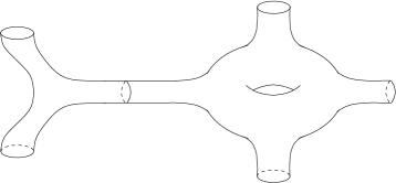
Figure 2: The origin of the massless poles in the five-graviton amplitude.

By extending the analysis in section 3.3, the limit as $v_{2}\to v_{1}$ identifies the massless pole in $s$ as

$$I_{12}\sim-\frac{1}{s}\cdot\frac{2}{\pi}\int_{\cal F}\!\frac{d^{2}\tau}{({\rm Im}\,\tau)^{5}}\int_{\cal T}\prod_{r=2}^{4}d^{2}v_{r}{\prod_{\begin{subarray}{c}r<s\\ 1\to 2\end{subarray}}}^{\prime}(\chi_{rs})^{\frac{1}{2}k_{r}\cdot k_{s}},$$ (69)

where the prime indicates that $(r,s)=(1,2)$ is not to be included, and $1\to 2$ means that $v_{1}$ is to be replaced by $v_{2}$ everywhere within the product. This product can be rewritten without the prime as $\prod_{r<s}(\chi_{rs})^{\frac{1}{2}k_{r}^{\prime}\cdot k_{s}^{\prime}}$, where $r,\,s$ now run only from $1$ to $4$ and where

$$k_{1}^{\prime}=k_{1}+k_{2},\qquad k_{2}^{\prime}=k_{3},\qquad k_{3}^{\prime}=k_{4},\qquad k_{4}^{\prime}=k_{5}.$$ (70)

It is now easy to recognise the residue of the pole as the product of a tree-level three-graviton vertex and a four-graviton one-loop amplitude, as required by unitarity. The poles for other values of $r$ and $s$ work in an identical manner.

4.3 Expansion of Integral $K$

First we expand integral $K$ since this is most similar to the integral in the four-graviton case. Ignoring the irrelevant delta function in (3.1.3),

$$K=-\frac{1}{2\pi}\int_{\cal F}\!\frac{d^{2}\tau}{({\rm Im}\,\tau)^{6}}\int_{\cal T}\prod_{r^{\prime}=1}^{4}d^{2}v_{r^{\prime}}\prod_{r^{\prime}<s^{\prime}}(\chi_{r^{\prime}s^{\prime}})^{\frac{1}{2}k_{r^{\prime}}\cdot k_{s^{\prime}}},$$ (71)

where the product over $\chi$’s can be written in terms of independent Mandelstam variables as

$$\left(\frac{\chi_{12}\chi_{35}\chi_{45}}{\chi_{15}\chi_{25}\chi_{34}}\right)^{-\frac{1}{4}s}\left(\frac{\chi_{13}\chi_{45}}{\chi_{15}\chi_{34}}\right)^{-\frac{1}{4}t}\left(\frac{\chi_{14}\chi_{35}}{\chi_{15}\chi_{34}}\right)^{-\frac{1}{4}u}\left(\frac{\chi_{23}\chi_{45}}{\chi_{25}\chi_{34}}\right)^{-\frac{1}{4}v}\left(\frac{\chi_{24}\chi_{35}}{\chi_{25}\chi_{34}}\right)^{-\frac{1}{4}w}.$$ (72)

By studying $v_{r}\to v_{s}$, it is easy to show that there are no massless poles.

Since none of the $v_{r}$ play a privileged rôle in the integrand of $K$, the low-energy expansion will be symmetric in the variables $k_{r}\cdot k_{s}$ and so we require the most general symmetric expressions at each order. At order $\alpha^{\prime 2}$ there are three potential candidates, which are in fact all proportional to each other,

$$(k_{1}\cdot k_{2})^{2}+(k_{1}\cdot k_{3})^{2}+\cdots+(k_{4}\cdot k_{5})^{2} \equiv X,$$

$$(k_{1}\cdot k_{2})(k_{1}\cdot k_{3})+\cdots+(k_{3}\cdot k_{5})(k_{4}\cdot k_{5}) =-X,$$

$$(k_{1}\cdot k_{2})(k_{3}\cdot k_{4})+\cdots+(k_{2}\cdot k_{5})(k_{3}\cdot k_{4}) ={\textstyle\frac{1}{2}}X.$$ (73)

At order $\alpha^{\prime 3}$ there are many more symmetric expressions, but again it can be shown that they are all proportional to each other, so that we are free to choose $\sum_{r<s}(k_{r}\cdot k_{s})^{3}$ as the only independent combination. Then the most general expansion for $K$ up to order $\alpha^{\prime 3}$ is given by

$$K =a+b\sum_{r<s}k_{r}\cdot k_{s}+c\sum_{r<s}(k_{r}\cdot k_{s})^{2}+d\sum_{r<s}(k_{r}\cdot k_{s})^{3}$$

$$=a+\frac{c}{4}(6s^{2}+4t^{2}+6st+\cdots)+\frac{d}{8}(6t^{2}u+\cdots),$$ (74)

where the second term has been dropped since it vanishes using momentum conservation. Threshold terms have been ignored since these will be removed by imposing ${\rm Im}\,\tau<L$ on the fundamental domain.

The value of $a$ is found simply by setting $s=t=u=v=w=0$, giving

$$a=-\frac{1}{2\pi}\int_{\cal F}\!\frac{d^{2}\tau}{({\rm Im}\,\tau)^{6}}\int_{\cal T}\prod_{r^{\prime}=1}^{4}d^{2}v_{r^{\prime}}=-\frac{1}{2\pi}\int_{\cal F}\!\frac{d^{2}\tau}{({\rm Im}\,\tau)^{2}}=-\frac{1}{6}.$$ (75)

Using (4.3), the value of $c$ can be found in many ways, all, of course, giving the same result. For example,

$$c =\lim_{s,t,\ldots\to 0}\left(\frac{1}{2}\frac{\partial^{2}K}{\partial t^{2}}\right)\bigg{|}_{\rm const}$$

$$=-\frac{1}{2^{6}\pi}\int_{\cal F}\!\frac{d^{2}\tau}{({\rm Im}\,\tau)^{6}}\int_{\cal T}\prod_{r^{\prime}=1}^{4}d^{2}v_{r^{\prime}}\,(\ln\chi_{13}+\ln\chi_{45}-\ln\chi_{15}-\ln\chi_{34})^{2}\,\bigg{|}_{\rm const}.$$ (76)

After expanding the bracket only the square terms will give non-zero contributions. For example, $\int_{\cal T}\prod_{r^{\prime}=1}^{4}d^{2}v_{r^{\prime}}\ln\chi_{13}\ln\chi_{45}$ vanishes since the integral of a single $\ln\chi$ is zero. By changing variables and performing three of the $v_{r^{\prime}}$-integrals,

$$c=-\frac{1}{2^{4}\pi}\int_{\cal F}\!\frac{d^{2}\tau}{({\rm Im}\,\tau)^{3}}\int_{\cal T}d^{2}v(\ln\chi)^{2}\,\bigg{|}_{\rm const}\equiv-\frac{1}{2^{4}\pi}\Theta_{1}|_{\rm const},$$ (77)

where the last part defines $\Theta_{1}$. The integral $\Theta_{1}$ is exactly the same as that encountered in section 2.1.1 and when the remaining $v$-integral is performed we again find the Epstein zeta function $Z_{2}(\tau,\bar{\tau})$. Following the same analysis, the $\tau$-integral over the ${\rm Im}\,\tau<L$ region of the fundamental domain gives

$$c_{L}=-\frac{\pi}{2^{2}\cdot 6!}L+\mathcal{O}(L^{-2})\quad\Rightarrow\quad c=0,$$ (78)

where the final part follows since $L$-dependent parts of $c_{L}$ must cancel with the same integral over the upper part of the fundamental domain.

Finding $d$ involves a similar calculation. For example,

$$d =\frac{2}{3}\lim_{s,t,\ldots\to 0}\frac{\partial^{3}K}{\partial t^{2}\partial u}\bigg{|}_{\rm const}$$

$$=\frac{1}{2^{6}\cdot 3\pi}\int_{\cal F}\!\frac{d^{2}\tau}{({\rm Im}\,\tau)^{6}}\int_{\cal T}\prod_{r^{\prime}=1}^{4}d^{2}v_{r^{\prime}}\,(\ln\chi_{13}+\ln\chi_{45}-\ln\chi_{15}-\ln\chi_{34})^{2}$$

$$\qquad\qquad\times(\ln\chi_{14}+\ln\chi_{35}-\ln\chi_{15}-\ln\chi_{34})\,\Big{|}_{\rm const}.$$ (79)

There are only two non-vanishing contributions: eight terms containing $\ln\chi_{rs}\ln\chi_{st}\ln\chi_{tr}$ and two terms containing $(\ln\chi_{rs})^{3}$. After performing the $v$-integrals for the first kind, the contribution to $d$ is given by

$$-\frac{1}{2^{3}\cdot 3\pi}\int_{\cal F}\!\frac{d^{2}\tau}{({\rm Im}\,\tau)^{4}}\int_{\cal T}d^{2}v_{1}d^{2}v_{2}\left(\ln\chi_{1}\ln\chi_{2}\ln\chi_{1+2}\right)\equiv-\frac{1}{2^{3}\cdot 3\pi}\Theta_{2},$$ (80)

which defines $\Theta_{2}$ and where $\ln\chi_{1+2}$ means $\ln\chi(v_{1}+v_{2},\tau)$. The same integral was found in section 2.1.2 where it was shown to involve the zeta function $Z_{3}(\tau,\bar{\tau})$. As there, the $\tau$-integral can be converted to an integral over the boundary of the restricted fundamental domain which again leads to $L$-dependent terms, but no constant piece. So $d$ is given entirely by the second type of term,

$$d=-\frac{1}{2^{5}\cdot 3\pi}\int_{\cal F}\!\frac{d^{2}\tau}{({\rm Im}\,\tau)^{3}}\int_{\cal T}d^{2}v(\ln\chi)^{3}\,\bigg{|}_{\rm const}\equiv-\frac{1}{2^{5}\cdot 3\pi}\Theta_{3}|_{\rm const}.$$ (81)

The integral $\Theta_{3}$ was also encountered in section 2.1.2 and, using the same ‘unfolding procedure’ as in [20], it is easy to show that

$$\Theta_{3}|_{\rm const}=-\frac{\zeta(2)\zeta(3)}{4\pi}.$$ (82)

So, up to order $\alpha^{\prime 3}$ and ignoring threshold corrections, the expansion of $K$ is given by

$$K=-\frac{1}{6}+\frac{\zeta(3)\alpha^{\prime 3}}{2^{5}\cdot 3^{2}}\sum_{r<s}(k_{r}\cdot k_{s})^{3}+\mathcal{O}(\alpha^{\prime 4}),$$ (83)

where $\alpha^{\prime}$ has been reinstated using $2\alpha^{\prime}=1$.

4.4 Expansion of Integral $J$

Now consider the integral $J_{rs|rt}$, which only needs to be expanded up to order $\alpha^{\prime 2}$. For concreteness consider $J_{12|13}$. Then, using (3.1.2) and changing variables so that $v_{12}\to v_{1}$, $v_{13}\to v_{2}$,

$$J_{12|13} =\frac{1}{\pi^{2}}\int_{\cal F}\!\frac{d^{2}\tau}{({\rm Im}\,\tau)^{5}}\int_{\cal T}\prod_{r^{\prime}=1}^{4}d^{2}v_{r^{\prime}}\,\frac{\partial}{\partial v}(\ln\chi_{1})\frac{\partial}{\partial\bar{v}}(\ln\chi_{2})$$

$$\qquad\times\left(\frac{\ln\chi_{1}\ln\chi_{3}\ln\chi_{4}}{\ln\chi_{2+3}\ln\chi_{-1+2+3}\ln\chi_{3-4}}\right)^{-\frac{1}{4}s}\left(\frac{\ln\chi_{2}\ln\chi_{4}}{\ln\chi_{2+3}\ln\chi_{3-4}}\right)^{-\frac{1}{4}t}$$

$$\qquad\times\left(\frac{\ln\chi_{2+3-4}\ln\chi_{3}}{\ln\chi_{2+3}\ln\chi_{3-4}}\right)^{-\frac{1}{4}u}\left(\frac{\ln\chi_{-1+2}\ln\chi_{4}}{\ln\chi_{-1+2+3}\ln\chi_{3-4}}\right)^{-\frac{1}{4}v}\left(\frac{\ln\chi_{-1+2+3-4}\ln\chi_{3}}{\ln\chi_{-1+2+3}\ln\chi_{3-4}}\right)^{-\frac{1}{4}w},$$ (84)

where, due to the periodicity of the integrand, there is no change to the $v_{r}$ integration region. The absence of massless poles can again be shown by studying the $v_{rs}\to 0$ limit.

Unlike $K$, $v_{rs}$ and $v_{rt}$ now play a privileged rôle in the definition of $J_{rs|rt}$ and so the expansion is expected to have less symmetry. However, $J_{12|13}$ should still be symmetric under $k_{4}\leftrightarrow k_{5}$ and, assuming it is real, under $k_{2}\leftrightarrow k_{3}$. This symmetry is manifest when the expansion is written in terms of $k_{r}\cdot k_{s}$, which is also the form required for comparing with the effective action. However, in practice we determine the expansion in terms of the independent Mandelstam variables $s$, $t$, $u$, $v$ and $w$, for which any symmetry is lost, and then deduce the expansion in terms of $k_{r}\cdot k_{s}$. So we must consider the most general form for the expansion up to order $\alpha^{\prime 2}$,

$$J_{12|13} =\>a$$

$$\quad+b_{1}s+b_{2}t+b_{3}u+b_{4}v+b_{5}w$$

$$\quad+c_{1}s^{2}+c_{2}t^{2}+c_{3}u^{2}+c_{4}v^{2}+c_{5}w^{2}$$

$$\quad+d_{1}st+d_{2}su+d_{3}sv+d_{4}sw+d_{5}tu+d_{6}tv+d_{7}tw+d_{8}uv+d_{9}uw+d_{10}vw,$$ (85)

where, as usual, we have ignored non-analytic terms.

The constant $a$ is easily found by setting all the Mandelstam variables to zero, leaving an expression involving the integral $\int_{\cal T}d^{2}v\frac{\partial}{\partial v}(\ln\chi)$. Although the integrand is infinite at $v=0$, the integral itself is finite, as can be seen by writing $d^{2}v$ as $|v|d|v|d\theta$ and, in fact, vanishes due to the antisymmetry of $\partial_{v}\ln\chi$ under $v\to-v$.

The coefficients $b_{i}$ are determined by considering single derivatives of (4.4) with respective to some Mandelstam variable. For example,

$$b_{1} =\lim_{s,t,\ldots\to 0}\frac{\partial J}{\partial s}\bigg{|}_{\rm const}$$

$$=-\frac{1}{4\pi^{2}}\int_{\cal F}\!\frac{d^{2}\tau}{({\rm Im}\,\tau)^{5}}\int_{\cal T}\prod_{r^{\prime}=1}^{4}d^{2}v_{r^{\prime}}\,\frac{\partial}{\partial v}(\ln\chi_{1})\frac{\partial}{\partial\bar{v}}(\ln\chi_{2})$$

$$\qquad\quad\times\big{(}\ln\chi_{1}+\ln\chi_{3}+\ln\chi_{4}-\ln\chi_{2+3}-\ln\chi_{-1+2+3}-\ln\chi_{3-4}\big{)}\,\Big{|}_{\rm const},$$ (86)

where all the terms vanish since they all contain $\int_{\cal T}d^{2}v\,\partial_{v}\ln\chi$ factors. (To see this for the fifth term it is necessary to change variables so that $-v_{1}+v_{2}+v_{3}\to v_{3}$.) Similarly $b_{2}$, $b_{3}$ and $b_{5}$ all vanish. However, $b_{4}$ is potentially non-zero,

$$b_{4}=\frac{1}{4\pi^{2}}\int_{\cal F}\!\frac{d^{2}\tau}{({\rm Im}\,\tau)^{3}}\int_{\cal T}d^{2}v_{1}d^{2}v_{2}\,\frac{\partial}{\partial v}(\ln\chi_{1})\frac{\partial}{\partial\bar{v}}(\ln\chi_{2})\ln\chi_{1+2}\,\bigg{|}_{\rm const}\equiv\frac{1}{4\pi^{2}}\Theta_{4}|_{\rm const}.$$ (87)

It is worth noting that, despite appearances, $\Theta_{4}$ is still modular invariant since the constant term added to $\ln\chi_{1+2}$ under a modular transformation vanishes by the antisymmetry of $\partial_{v}\ln\chi$. After performing the $v$-integrals, the same zeta function $Z_{2}(\tau,\bar{\tau})$ is found as at order $\alpha^{\prime 2}$ in the expansion of $K$, despite originating from a different integral. In fact, $\Theta_{4}=\frac{1}{2}\pi\Theta_{1}$. Since $\Theta_{1}$ only leads to $L$-dependent terms with no constant part, we can conclude that $b_{4}=0$.

The $c_{i}$ and $d_{i}$ coefficients can be found in a similar manner giving

$$c_{1}=\frac{1}{16\pi^{2}}\Theta_{5}|_{\rm const},\quad c_{2}=0,\quad c_{3}=0,\quad c_{4}=-\frac{1}{32\pi^{2}}\Theta_{6}|_{\rm const},\quad c_{5}=\frac{1}{8\pi^{2}}\Theta_{5}|_{\rm const},$$ (88)

and

$$d_{1} =0, d_{2} =\frac{1}{16\pi^{2}}\Theta_{5}|_{\rm const}, d_{3} =\frac{1}{16\pi^{2}}(\Theta_{5}|_{\rm const}-\Theta_{7}|_{\rm const}),$$

$$d_{4} =\frac{3}{16\pi^{2}}\Theta_{5}|_{\rm const}, d_{5} =0, d_{6} =-\frac{1}{16\pi^{2}}\Theta_{8}|_{\rm const},$$

$$d_{7} =\frac{1}{16\pi^{2}}\Theta_{5}|_{\rm const}, d_{8} =\frac{1}{16\pi^{2}}\Theta_{5}|_{\rm const}, d_{9} =\frac{1}{8\pi^{2}}\Theta_{5}|_{\rm const},$$

$$d_{10} =\frac{1}{8\pi^{2}}\Theta_{5}|_{\rm const},$$ (89)

where

$$\Theta_{5} \equiv\int_{\cal F}\!\frac{d^{2}\tau}{({\rm Im}\,\tau)^{4}}\int_{\cal T}d^{2}v_{1}d^{2}v_{2}d^{2}v_{3}\,\frac{\partial}{\partial v}(\ln\chi_{1})\frac{\partial}{\partial\bar{v}}(\ln\chi_{2})\ln\chi_{1+2+3}\ln\chi_{3},$$

$$\Theta_{6} \equiv\int_{\cal F}\!\frac{d^{2}\tau}{({\rm Im}\,\tau)^{3}}\int_{\cal T}d^{2}v_{1}d^{2}v_{2}\,\frac{\partial}{\partial v}(\ln\chi_{1})\frac{\partial}{\partial\bar{v}}(\ln\chi_{2})(\ln\chi_{1+2})^{2},$$

$$\Theta_{7} \equiv\int_{\cal F}\!\frac{d^{2}\tau}{({\rm Im}\,\tau)^{3}}\int_{\cal T}d^{2}v_{1}d^{2}v_{2}\,\frac{\partial}{\partial v}(\ln\chi_{1})\frac{\partial}{\partial\bar{v}}(\ln\chi_{2})\ln\chi_{1}\ln\chi_{1+2},$$

$$\Theta_{8} \equiv\int_{\cal F}\!\frac{d^{2}\tau}{({\rm Im}\,\tau)^{3}}\int_{\cal T}d^{2}v_{1}d^{2}v_{2}\,\frac{\partial}{\partial v}(\ln\chi_{1})\frac{\partial}{\partial\bar{v}}(\ln\chi_{2})\ln\chi_{2}\ln\chi_{1+2}.$$ (90)

Despite involving different integrands, performing the $v_{r}$-integrals shows that $\Theta_{5}$ and $\Theta_{6}$ involve the same modular functions encountered in calculating $d$ in the expansion of $K$. In fact, $\Theta_{5}=\frac{\pi}{2}\Theta_{2}$ and $\Theta_{6}=\frac{\pi}{2}\Theta_{3}$ and so, after performing the $\tau$-integrals, we find

$$\Theta_{5}|_{\rm const}=0,\qquad\Theta_{6}|_{\rm const}=-\frac{\zeta(2)\zeta(3)}{8}.$$ (91)

However, $\Theta_{7}$ and $\Theta_{8}$ do lead to new expressions,

$$\Theta_{7} =-\frac{1}{16\pi^{2}}\int_{\cal F}\!\frac{d^{2}\tau}{({\rm Im}\,\tau)^{2}}\sum_{(m,n),(p,q),(r,s)\neq(0,0)}\frac{({\rm Im}\,\tau)^{3}\,\delta_{m+r-p}\delta_{n+s-q}}{(m\tau+n)(p\bar{\tau}+q)|r\tau+s|^{2}|p\tau+q|^{2}},$$

$$\Theta_{8} =-\frac{1}{16\pi^{2}}\int_{\cal F}\!\frac{d^{2}\tau}{({\rm Im}\,\tau)^{2}}\sum_{(m,n),(p,q),(r,s)\neq(0,0)}\frac{({\rm Im}\,\tau)^{3}\,\delta_{m+r-p}\delta_{n+s-q}}{(m\tau+n)(p\bar{\tau}+q)|r\tau+s|^{2}|m\tau+n|^{2}}.$$ (92)

As with $\Theta_{3}$ (and $\Theta_{6}$), there is no obvious way to write the integrands as total derivatives. Perhaps an ‘unfolding procedure’ could be used as in [20]. However, it is not necessary to explicitly evaluate them since their constant parts will be inferred as follows. The same integrals will appear in the pole terms of the expansion of integral $I_{rs}$. However, these poles are completely fixed by unitarity and this will allow $\Theta_{7}$ and $\Theta_{8}$ to be uniquely determined. For completeness we state here that we will find

$$\Theta_{7}|_{\rm const}=\Theta_{8}|_{\rm const}={\textstyle\frac{1}{2}}\Theta_{6}|_{\rm const}=-\frac{\zeta(2)\zeta(3)}{16}.$$ (93)

Having determined all the coefficients, we can now write

$$J_{12|13} =\frac{\Theta_{4}|_{\rm const}}{4\pi^{2}}v$$

$$\quad+\frac{\Theta_{5}|_{\rm const}}{16\pi^{2}}(s^{2}+2w^{2}+su+3sw+tw+uv+2uw+2vw)$$

$$\quad-\frac{\Theta_{6}|_{\rm const}}{32\pi^{2}}v^{2}+\frac{\Theta_{5}|_{\rm const}-\Theta_{7}|_{\rm const}}{16\pi^{2}}sv-\frac{\Theta_{8}|_{\rm const}}{16\pi^{2}}tv$$

$$\quad+\mathcal{O}(\alpha^{\prime 3}),$$ (94)

which now needs to be rewritten in terms of $k_{r}\cdot k_{s}$ and generalised to $J_{rs|rt}$. For some terms this is trivial. For example, it is clear that the $v$ multiplying $\Theta_{4}|_{\rm const}$ should be generalised to $-2k_{s}\cdot k_{t}$. Other terms are more tricky although, by considering various other values for $r,\,s,\,t$, it can be shown that, up to order $\alpha^{\prime 2}$,

$$J_{rs|rt} =-\frac{\Theta_{4}|_{\rm const}}{2\pi^{2}}k_{s}\cdot k_{t}$$

$$\quad+\frac{\Theta_{5}|_{\rm const}-\frac{1}{2}\Theta_{6}|_{\rm const}}{4\pi^{2}}(k_{s}\cdot k_{t})^{2}+\frac{\Theta_{5}|_{\rm const}}{4\pi^{2}}(k_{r}\cdot k_{u})(k_{r}\cdot k_{v})$$

$$\quad+\frac{\Theta_{5}|_{\rm const}-\Theta_{7}|_{\rm const}}{4\pi^{2}}(k_{r}\cdot k_{s})(k_{s}\cdot k_{t})+\frac{\Theta_{5}|_{\rm const}-\Theta_{8}|_{\rm const}}{4\pi^{2}}(k_{r}\cdot k_{t})(k_{s}\cdot k_{t})$$

$$\quad-\frac{\Theta_{5}|_{\rm const}}{4\pi^{2}}\big{(}(k_{s}\cdot k_{u})(k_{s}\cdot k_{v})+(k_{s}\cdot k_{u})(k_{t}\cdot k_{u})+(k_{s}\cdot k_{u})(k_{t}\cdot k_{v})$$

$$\qquad\qquad\qquad+(k_{s}\cdot k_{v})(k_{t}\cdot k_{u})+(k_{s}\cdot k_{v})(k_{t}\cdot k_{v})+(k_{t}\cdot k_{u})(k_{t}\cdot k_{v})\big{)},$$ (95)

where $k_{u}$, $k_{v}$ are the two momenta other than $k_{r}$, $k_{s}$, $k_{t}$. Only $\Theta_{6}$, $\Theta_{7}$ and $\Theta_{8}$ have non-zero constant parts and so, using (93) and reinstating $\alpha^{\prime}$, this simplifies to

$$J_{rs|rt}=\frac{\zeta(3)\alpha^{\prime 2}}{2^{5}\cdot 3}(k_{s}\cdot k_{t})(k_{s}\cdot k_{t}+k_{r}\cdot k_{s}+k_{r}\cdot k_{t})+\mathcal{O}(\alpha^{\prime 3}).$$ (96)

4.5 Expansion of Integral $J^{\prime}$

Integral $J^{\prime}$ differs from $J$ in that all of the indices on the $\eta\bar{\eta}$ are different. Specialising to the case $r,s=1,2$ and $t,u=3,4$, we have

$$J^{\prime}_{12|34}=\frac{1}{\pi^{2}}\int_{\cal F}\!\frac{d^{2}\tau}{({\rm Im}\,\tau)^{5}}\int_{\cal T}\prod_{r^{\prime}=1}^{4}d^{2}v_{r^{\prime}}\prod_{r^{\prime}<s^{\prime}}(\chi_{r^{\prime}s^{\prime}})^{\frac{1}{2}k_{r^{\prime}}\cdot k_{s^{\prime}}}\frac{\partial}{\partial v}(\ln\chi_{12})\frac{\partial}{\partial\bar{v}}(\ln\chi_{34}).$$ (97)

Again, studying the region $v_{rs}\to 0$ shows the absence of massless poles. This completes our earlier claim that the only source of massless poles is integral $I$.

As with $J$, we begin with the most general possible expansion given in (4.4). The details are identical in spirit to those in section 4.4 and are not presented here. It is found that, up to and including order $\alpha^{\prime 2}$, all coefficients vanish except

$$d_{7}=-\frac{1}{16\pi^{2}}\Theta_{5}|_{\rm const},\qquad d_{8}=\frac{1}{16\pi^{2}}\Theta_{5}|_{\rm const}.$$ (98)

This is easily extended to general $r,\,s,\,t,\,u$, giving

$$J^{\prime}_{rs|tu}=-\frac{\Theta_{5}|_{\rm const}}{4\pi^{2}}\big{(}(k_{r}\cdot k_{t})(k_{s}\cdot k_{u})-(k_{r}\cdot k_{u})(k_{s}\cdot k_{t})\big{)}.$$ (99)

Since $\Theta_{5}$ has no non-zero constant part, we conclude that

$$J^{\prime}_{rs|tu}=0+\mathcal{O}(\alpha^{\prime 3}).$$ (100)

Although $J^{\prime}$ vanishes at all orders considered in this paper, it is not identically zero and will start to contribute at some higher order. The effect of its vanishing up to order $\alpha^{\prime 2}$ is that the effective action can be written as $t_{8}t_{8}(D^{2n}R^{3})(R^{2})$, where the final two Riemann tensors contract straight into the $t_{8}$ tensors. At higher orders, when $J^{\prime}$ starts to contribute, this will no longer be the case.

4.6 Expansion of Integral $I$

As it stands, the low-energy expansion of $I$ makes little sense. However, after removing the poles the integral become finite for vanishing momenta and so can be expanded for small $k_{r}\cdot k_{s}$. Consider the case where $r,s=1,2$,

$$I_{12}=\frac{1}{\pi^{2}}\int_{\cal F}\!\frac{d^{2}\tau}{({\rm Im}\,\tau)^{5}}\int_{\cal T}\prod_{r^{\prime}=1}^{4}d^{2}v_{r^{\prime}}\prod_{r^{\prime}<s^{\prime}}(\chi_{r^{\prime}s^{\prime}})^{\frac{1}{2}k_{r^{\prime}}\cdot k_{s^{\prime}}}\frac{\partial}{\partial{v}}(\ln\chi_{12})\frac{\partial}{\partial\bar{v}}(\ln\chi_{12}).$$ (101)

Since the poles are known from section 4.2, they can, in principle, be subtracted order by order in $\alpha^{\prime}$. Although some progress can be made this way, it becomes increasingly difficult to find suitable representations for the pole terms. Instead we use an alternative method which allows $I$ to be directly expressed in terms of the integrals $J$ and $K$.

Consider the following integral,

$$\frac{1}{\pi^{2}}\int_{\cal F}\!\frac{d^{2}\tau}{({\rm Im}\,\tau)^{5}}\int_{\cal T}\prod_{r^{\prime}=1}^{4}d^{2}v_{r^{\prime}}\,\frac{\partial}{\partial\bar{v}_{1}}\left(\prod_{r^{\prime}<s^{\prime}}(\chi_{r^{\prime}s^{\prime}})^{\frac{1}{2}k_{r^{\prime}}\cdot k_{s^{\prime}}}\frac{\partial}{\partial v}\ln\chi_{12}\right),$$ (102)

which vanishes since $v_{r}$ is integrated over a surface with no boundary. (The potential singularity near $|v_{12}|=0$ is easily shown to be finite in the limit $s\to 0$.) By acting with the $\bar{v}_{1}$ derivative, various $I$, $J$ and $K$ integrals are generated, leading to the relation

$$I_{12}=-\frac{k_{1}\cdot k_{3}}{k_{1}\cdot k_{2}}J_{12|13}-\frac{k_{1}\cdot k_{4}}{k_{1}\cdot k_{2}}J_{12|14}-\frac{k_{1}\cdot k_{5}}{k_{1}\cdot k_{2}}J_{12|15}-\frac{2}{k_{1}\cdot k_{2}}K,$$ (103)

which clearly only contains single poles in $k_{1}\cdot k_{2}$. For general $r$, $s$ the result is generalised to

$$I_{rs}=-\sum_{t=1,\,t\neq r,s}^{5}\frac{k_{r}\cdot k_{t}}{k_{r}\cdot k_{s}}J_{rs|rt}-\frac{1}{\alpha^{\prime}k_{r}\cdot k_{s}}K,$$ (104)

where $\alpha^{\prime}$ has been reinserted. The expansion of $I$ is then easily obtained using the expansions of $J$ and $K$ given in (4.4) and (83) respectively. At order $\alpha^{\prime-1}$ we find $\frac{1}{6\alpha^{\prime}k_{r}\cdot k_{s}}$, agreeing with the lowest order expansion of (69). Orders $\alpha^{\prime 0}$ and $\alpha^{\prime 1}$ vanish. The next order contribution, after separating poles and non-poles, is

$$\frac{\alpha^{\prime 2}}{6\pi^{2}(k_{r}\cdot k_{s})}\Bigg{(}\sum_{t\neq r,s}\Big{(}3(k_{r}\cdot k_{t})(k_{s}\cdot k_{t})^{2}\Theta_{6}|_{\rm const}+6(k_{r}\cdot k_{t})^{2}(k_{s}\cdot k_{t})\Theta_{8}|_{\rm const}\Big{)}$$

$$\qquad\qquad\qquad+\sum_{(t,u)\neq(r,s)}(k_{t}\cdot k_{u})^{3}\Theta_{6}|_{\rm const}\Bigg{)}$$

$$\qquad\,+\frac{\alpha^{\prime 2}}{6\pi^{2}}\Bigg{(}6\sum_{t\neq r,s}(k_{r}\cdot k_{t})(k_{s}\cdot k_{t})\Theta_{7}|_{\rm const}+(k_{r}\cdot k_{s})^{2}\Theta_{6}|_{\rm const}\Bigg{)},$$ (105)

where we have not assumed any relationship between $\Theta_{6}$, $\Theta_{7}$ and $\Theta_{8}$. From unitarity we know that the kinematic factor multiplying the pole must involve the expansion of the four-graviton amplitude to third order, which is

$$\sum_{t\neq r,s}\big{(}(k_{r}+k_{s})\cdot k_{t}\big{)}^{3}+\sum_{(t,u)\notin\{r,s\}}\big{(}k_{t}\cdot k_{u}\big{)}^{3},$$ (106)

where each sum contains three terms. Matching the two requires $2\Theta_{8}|_{\rm const}=\Theta_{6}|_{\rm const}$, confirming the claim in (93). The remaining relationship of (93), which involves $\Theta_{7}$, is shown in the same way but with $\partial_{v}$ interchanged with $\bar{\partial}_{v}$ in (102).

Using (91), our final expression for the expansion of $I_{rs}$ up to order $\alpha^{\prime 2}$ is

$$I_{rs} =\frac{1}{6\alpha^{\prime}k_{r}\cdot k_{s}}$$

$$\quad-\frac{\zeta(3)\alpha^{\prime 2}}{2^{5}\cdot 3^{2}(k_{r}\cdot k_{s})}\Bigg{(}\sum_{t\neq r,s}\big{(}(k_{r}+k_{s})\cdot k_{t}\big{)}^{3}+\sum_{t,u\notin\{r,s\}}\big{(}k_{t}\cdot k_{u}\big{)}^{3}\Bigg{)}$$

$$\quad-\frac{\zeta(3)\alpha^{\prime 2}}{2^{5}\cdot 3^{2}}\Bigg{(}3\sum_{t\neq r,s}(k_{r}\cdot k_{t})(k_{s}\cdot k_{t})+(k_{r}\cdot k_{s})^{2}\Bigg{)},$$ (107)

where the first line is the lowest-order pole, the second line is the order $\alpha^{\prime 2}$ pole, and the third line is the order $\alpha^{\prime 2}$ non-pole.

5 Consequences for the Effective Action

Given the low-energy expansion of the five-graviton amplitude, we can now determine whether this implies new terms in the type II effective action. As reviewed in section 2.2, the one-loop four-graviton amplitude implies the following one-loop terms in the effective action up to order $D^{6}R^{4}$,

$$\alpha^{\prime 3}\int d^{10}x\sqrt{-g}\left(4\zeta(2)e^{\phi/2}{\mathcal{R}^{4}}+0\cdot e^{-\phi/2}\alpha^{\prime 2}D^{4}{\mathcal{R}^{4}}+8\zeta(2)\zeta(3)e^{-\phi}\alpha^{\prime 3}D^{6}{\mathcal{R}^{4}}\right),$$ (108)

where we are now using Einstein frame since this simplifies the subsequent analysis. Using the four-graviton amplitude it is not possible to determine exactly how the derivatives are distributed amongst the Riemann tensors; for concreteness we assume $D^{2n}{\mathcal{R}^{4}}$ is shorthand for

$$t_{8}^{a_{1}b_{1}a_{2}b_{2}a_{3}b_{3}a_{4}b_{4}}t_{8}^{c_{1}d_{1}c_{2}d_{2}c_{3}d_{3}c_{4}d_{4}}((D^{2})^{n}(R_{a_{1}b_{1}c_{1}d_{1}}R_{a_{2}b_{2}c_{2}d_{2}}))\,R_{a_{3}b_{3}c_{3}d_{3}}R_{a_{4}b_{4}c_{4}d_{4}}.$$ (109)

By studying the five-graviton amplitude we can address three issues. Firstly, we can resolve the question about how the derivatives are distributed (modulo the $D^{2}R$ issue discussed below). Secondly, we can determine whether a $D^{2}R^{4}$ term exists, which cannot be seen from the four-graviton amplitude. Thirdly, we can study whether it is necessary to add new $R^{5}$, $D^{2}R^{5}$ and $D^{4}R^{5}$ terms.

The strategy will be to calculate the contribution to the five-graviton amplitude from (108) by expanding around flat space and considering all possible tree-level diagrams. After removing these diagrams, any remaining terms will be covariantised to find potentially novel $D^{2n}R^{5}$ terms.

5.1 Ambiguities in the Effective Action

As mentioned in the introduction, on-shell effective actions can only be determined up to field redefinitions. Since the Weyl tensor differs from the Riemann tensor by terms involving the Ricci tensor and Ricci scalar, it is impossible to distinguish the two, and $R^{4}$ can be replaced by $W^{4}$. This conclusion only holds if other fields, such as the $NS\otimes NS$ two-form and the $R\otimes R$ fields, are turned off. If they are not, then it is still true that $R^{4}$ and $W^{4}$ can be interchanged, but only at the expense of adding additional terms involving the other fields. Consequently, it may well be the case that either $R^{4}$ or $W^{4}$ is preferred since it leads to an effective action with fewer terms. For the case here, with all other fields turned off, we choose to use the Riemann tensor since its expansion around flat space is considerably simpler.

Now consider terms involving $D^{2}R_{abcd}$. By using the Bianchi identity and replacing $D_{[a}D_{b]}$ by Riemann tensors, it can be shown that

$$D^{2}R_{abcd} =2{R^{e}}_{afb}{R^{f}}_{ecd}-2{R^{e}}_{afc}{R^{f}}_{deb}+2{R^{e}}_{afd}{R^{f}}_{ceb}$$

$$\quad+R_{ae}{R^{e}}_{bcd}-R_{be}{R^{e}}_{acd}$$

$$\quad+D_{a}D_{c}R_{db}-D_{a}D_{d}R_{cb}-D_{b}D_{c}R_{da}+D_{b}D_{d}R_{ca},$$ (110)

and so, after removing the Ricci terms using a field redefinition, $D^{2}R_{abcd}$ can be replaced by a sum of Riemann-squared terms. This implies, for example, that $D^{2}{\mathcal{R}^{4}}$ can be replaced by a sum of $R^{5}$ terms (which is one explanation for why $D^{2}{\mathcal{R}^{4}}$ does not contribute to the four-graviton amplitude). Similarly

$$(D_{f}D_{e}R)(D^{e}D^{f}R^{3})=(D_{e}D_{f}R)(D^{e}D^{f}R^{3})+\mbox{``$D^{4}R^{5}$ terms''},$$ (111)

and so the issue of how the derivatives are distributed in $D^{2n}{\mathcal{R}^{4}}$ is actually ill-defined: different distributions are often equivalent up to $R^{5}$ terms. Then the only possible criteria for fixing the precise meaning of $D^{2n}{\mathcal{R}^{4}}$ involves choosing the term which leads to the fewest total number of terms in the effective action.

5.2 Expansions of Various Tensors

Before expanding (108), we first need to expand the Riemann, Ricci and $t_{8}$ tensors around flat space. Consider a small fluctuation of the metric about the Minkowski metric,

$$g_{ab}=\eta_{ab}+\kappa h_{ab},$$ (112)

where $\kappa$ is presumed small. In subsequent expressions we will drop factors of $\kappa$ since they can easily be reinstated; the order of the expansion is then given by the number of $h$ factors. Indices on $h$ and $\partial$ are raised and lowered with $\eta$, whereas all other indices are raised and lowered with $g$. So, for example,

$${\Gamma^{a}}_{bc}=g^{ad}\Gamma_{dbc},\qquad{h^{a}}_{b}=\eta^{ac}h_{cb},\qquad\partial^{a}=\eta^{ab}\partial_{b}.$$ (113)

The expansions of the inverse metric and the metric determinant are readily found to be

$$g^{ab} =\eta^{ab}-h^{ab}+h^{ac}{h_{c}}^{b}+\cdots,$$ (114)

$$\sqrt{-g} =1+{\textstyle\frac{1}{2}}{h^{a}}_{a}+\cdots,$$ (115)

and likewise for the Christoffel symbol,

$${\Gamma^{a}}_{bc}={\textstyle\frac{1}{2}}(\partial_{b}{h^{a}}_{c}+\partial_{c}{h^{a}}_{b}-\partial^{a}h_{bc})-{\textstyle\frac{1}{2}}h^{ad}(\partial_{b}h_{cd}+\partial_{c}h_{bd}-\partial_{d}h_{bc})+\cdots.$$ (116)

Since the expansion of $D^{2n}{\mathcal{R}^{4}}$ is required up to fifth order in $h$, we need the expansion of $R_{abcd}$ up to second order. After a slightly more involved calculation, it can be shown that

$$\eta^{ce}\eta^{df}R_{abef} =2\partial_{[a}\partial^{[c}{h_{b]}}^{d]}$$

$$\quad+\partial_{[a}h^{e[c}\partial^{d]}h_{b]e}+{\textstyle\frac{1}{2}}\partial_{[a}h^{ec}\partial_{b]}{h^{d}}_{e}+{\textstyle\frac{1}{2}}\partial^{[c}h_{ae}\partial^{d]}{h_{b}}^{e}$$

$$\quad-\partial^{e}{h_{[a}}^{[c}\partial_{b]}{h^{d]}}_{e}-\partial^{e}{h_{[a}}^{[c}\partial^{d]}h_{b]e}+{\textstyle\frac{1}{2}}\partial^{e}{h_{a}}^{[c}\partial_{e}{h^{d]}}_{b}.$$ (117)

Often the Riemann tensor $R_{abcd}$ is multiplied by $t_{8}^{ab\cdots}t_{8}^{cd\cdots}$ which is antisymmetric in $a\leftrightarrow b$ and in $c\leftrightarrow d$. This allows the first term to be rewritten as $2\partial_{a}\partial_{c}h_{bd}$, without the square brackets. Further, there is also a symmetry in $(a,\,b)\leftrightarrow(c,\,d)$. This symmetry is not obvious, but, since the ${\mathcal{R}^{4}}$ term is only expanded to fifth order, it follows that at least three Riemann tensors are only expanded to first order which, even when written as $2\partial_{a}\partial_{c}h_{bd}$, still has manifest $(a,\,b)\leftrightarrow(c,\,d)$ symmetry. With the understanding that $R_{abcd}$ is multiplied by a tensor with these symmetries, its expansion to second order simplifies to

$$R_{abcd}=2\partial_{a}\partial_{c}h_{bd}+\partial_{a}h_{c}^{\phantom{c}e}\partial_{d}h_{be}+\partial_{a}h_{c}^{\phantom{c}e}\partial_{b}h_{de}-2\partial^{e}h_{ac}\partial_{b}h_{de}+{\textstyle\frac{1}{2}}\partial^{e}h_{ac}\partial_{e}h_{bd}.$$ (118)

By contracting (5.2) with an inverse metric, the expansion of the Ricci tensor can be determined as

$$R_{ab} ={\textstyle\frac{1}{2}}(\Box h_{ab}+\partial_{a}\partial_{b}h-\partial_{a}\partial_{c}{h^{c}}_{b}-\partial_{b}\partial_{c}{h^{c}}_{a})$$

$$\quad-{\textstyle\frac{1}{2}}h^{cd}(\partial_{a}\partial_{b}h_{cd}+\partial_{c}\partial_{d}h_{ab}-\partial_{a}\partial_{c}h_{bd}-\partial_{b}\partial_{c}h_{ad})$$

$$\quad-{\textstyle\frac{1}{4}}\partial_{a}h_{cd}\partial_{b}h^{cd}+{\textstyle\frac{1}{2}}(\partial^{c}h_{ad}\partial^{d}h_{bc}-\partial_{c}h_{ad}\partial^{c}{h^{d}}_{b})$$

$$\quad+{\textstyle\frac{1}{4}}(\partial_{a}h_{bc}+\partial_{b}h_{ac}-\partial_{c}h_{ab})(2\partial_{d}h^{cd}-\partial^{c}h),$$ (119)

where $h={h^{a}}_{a}$ and $\Box=\partial^{a}\partial_{a}$. Similarly, the Ricci scalar is given by

$$R =\Box h-\partial_{a}\partial_{b}h^{ab}$$

$$\quad-h^{ab}(\Box h_{ab}+\partial_{a}\partial_{b}h-2\partial_{a}\partial^{c}h_{bc})$$

$$\quad-{\textstyle\frac{3}{4}}\partial_{a}h_{bc}\partial^{a}h^{bc}+{\textstyle\frac{1}{2}}\partial_{a}h_{bc}\partial^{b}h^{ac}+\partial^{a}h_{ab}\partial_{c}h^{bc}-\partial^{a}h_{ab}\partial^{b}h+{\textstyle\frac{1}{4}}\partial^{a}h\partial_{a}h.$$ (120)

We will actually need the Ricci scalar expanded to third order in $h$. This has previously been calculated in [40] and there is no need to reproduce the result here.

Finally, it is important to remember that the $t_{8}$ tensor must also be expanded. For the amplitudes calculated here, amplitudes in flat space, $t_{8}$ appears as a sum of products of inverse Minkowski metrics. However, when written in an effective action, $t_{8}$ is covariantised to involve full metrics and, as such, should be expanded in $h$. Where it is important to distinguish $t_{8}$ written in terms of the Minkowski metric from $t_{8}$ written in terms of the full metric we define

$$t_{8}^{abcdefgh} =\sum g^{\cdot\cdot}g^{\cdot\cdot}g^{\cdot\cdot}g^{\cdot\cdot}=-\frac{1}{2}g^{ac}g^{bd}g^{eg}g^{fh}+\mbox{59 other terms},$$

$$\underline{t}_{8}^{abcdefgh} =\sum\eta^{\cdot\cdot}\eta^{\cdot\cdot}\eta^{\cdot\cdot}\eta^{\cdot\cdot}=-\frac{1}{2}\eta^{ac}\eta^{bd}\eta^{eg}\eta^{fh}+\mbox{59 other terms}.$$ (121)

Then, to first order in $h$, $t_{8}$ can be expanded in terms of $\underline{t}_{8}$ as

$$t_{8}^{abcdefgh} =\underline{t}_{8}^{abcdefgh}$$

$$\quad-{\textstyle\frac{1}{2}}({h_{i}}^{a}\underline{t}_{8}^{ibcdefgh}+{h_{i}}^{b}\underline{t}_{8}^{aicdefgh}+{h_{i}}^{c}\underline{t}_{8}^{abidefgh}+{h_{i}}^{d}\underline{t}_{8}^{abciefgh}$$

$$\quad\qquad+h_{i}^{\phantom{i}e}\underline{t}_{8}^{abcdifgh}+{h_{i}}^{f}\underline{t}_{8}^{abcdeigh}+{h_{i}}^{g}\underline{t}_{8}^{abcdefih}+{h_{i}}^{h}\underline{t}_{8}^{abcdefgi}).$$ (122)

As with the Riemann tensor, $t_{8}$ is often multiplied by a tensor which is symmetric under the interchange of pairs of indices, e.g. under $(a,b)\leftrightarrow(c,d)$. For example, when ${\mathcal{R}^{4}}$ is expanded to fifth order, the lowest order expansion of the Riemann tensor, as shown in (118), has this symmetry. Then the expansion of $t_{8}$ simplifies to

$$t_{8}^{abcdefgh}=\underline{t}_{8}^{abcdefgh}-2({h_{i}}^{a}\underline{t}_{8}^{ibcdefgh}+{h_{i}}^{b}\underline{t}_{8}^{aicdefgh}).$$ (123)

5.3 Expansion of the Known Effective Action

We are now in a position to expand (108) up to fifth order. This will give the graviton propagator and various three-, four- and five-point vertices, some of which will be associated with tree-level terms and some with one-loop terms.

5.3.1 The Einstein-Hilbert Term

Consider first the Einstein-Hilbert action, $\int d^{10}x\sqrt{-g}R$. The first contribution, using (115) and (5.2) and dropping total derivatives, is at second order,

$$S_{EH}=\frac{1}{4}\int d^{10}x\,(\partial_{a}h_{bc}\partial^{a}h^{bc}-\partial_{a}h\partial^{a}h+2\partial_{a}h\partial_{b}h^{ab}-2\partial_{a}h_{bc}\partial^{b}h^{ac}),$$ (124)

which is invariant under the gauge transformation

$$h_{ab}\to h_{ab}+\partial_{a}\zeta_{b}+\partial_{b}\zeta_{a},$$ (125)

where $\zeta_{a}$ is an arbitrary one-form field. We fix the gauge invariance using the de Donder gauge, $\partial^{a}h_{ab}={\textstyle\frac{1}{2}}\partial_{b}h$, which leads to the usual graviton propagator,

$$D_{ab,cd}=\frac{\eta_{ac}\eta_{bd}+\eta_{ad}\eta_{bc}-\frac{1}{4}\eta_{ab}\eta_{cd}}{k^{2}}.$$ (126)

The expansion of $\sqrt{-g}R$ to third order gives a three-graviton vertex, $V_{3\,ab,cd,ef}^{R}$, which was first calculated in [40]. The result is not given here since we will take a short-cut when calculating diagrams involving such a vertex.

5.3.2 The ${\mathcal{R}^{4}}$ Term

Since each Riemann tensor contains at least one $h$, the expansion of $\int d^{10}x\sqrt{-g}\,{\mathcal{R}^{4}}$ begins at fourth order. With all tensors expanded to lowest order, the action becomes

$$S^{{\mathcal{R}^{4}}}_{4h}=2^{4}\int d^{10}x\,\underline{t}_{8}^{a_{1}b_{1}\cdots}\underline{t}_{8}^{c_{1}d_{1}\cdots}\partial_{a_{1}}\partial_{c_{1}}h_{b_{1}d_{1}}\,\partial_{a_{2}}\partial_{c_{2}}h_{b_{2}d_{2}}\,\partial_{a_{3}}\partial_{c_{3}}h_{b_{3}d_{3}}\,\partial_{a_{4}}\partial_{c_{4}}h_{b_{4}d_{4}}$$ (127)

and it is straightforward to read off the four-graviton vertex as

$$V^{{\mathcal{R}^{4}}}_{4\,ab,cd,ef,gh} =2^{4}\,\underline{t}_{8}^{a_{1}b_{1}a_{2}b_{2}a_{3}b_{3}a_{4}b_{4}}\underline{t}_{8}^{c_{1}d_{1}c_{2}d_{2}c_{3}d_{3}c_{4}d_{4}}\,k_{1\,a_{1}}k_{1\,c_{1}}k_{2\,a_{2}}k_{2\,c_{2}}k_{3\,a_{3}}k_{3\,c_{3}}k_{4\,a_{4}}k_{4\,c_{4}}$$

$$\qquad\times\eta_{b_{1}a}\eta_{d_{1}b}\eta_{b_{2}c}\eta_{d_{2}d}\eta_{b_{3}e}\eta_{d_{3}f}\eta_{b_{4}g}\eta_{d_{4}h}.$$ (128)

Expanding to fifth order is more involved. The fifth graviton can originate either from the $\sqrt{-g}$, from a $t_{8}$ tensor or from a Riemann tensor. When it originates from the $\sqrt{-g}$, the term will necessarily involve a $\frac{1}{2}h$ factor, which can be ignored for our purposes since this vertex will only ever be used in diagrams with all legs on-shell. With this understanding,

$$S^{{\mathcal{R}^{4}}}_{5h} =2^{5}\int d^{10}x\,\underline{t}_{8}^{a_{1}b_{1}a_{2}b_{2}a_{3}b_{3}a_{4}b_{4}}\underline{t}_{8}^{c_{1}d_{1}c_{2}d_{2}c_{3}d_{3}c_{4}d_{4}}\partial_{a_{2}}\partial_{c_{2}}h_{b_{2}d_{2}}\,\partial_{a_{3}}\partial_{c_{3}}h_{b_{3}d_{3}}\,\partial_{a_{4}}\partial_{c_{4}}h_{b_{4}d_{4}}$$

$$\qquad\times(-\partial_{a_{1}}{h_{d_{1}}}^{e}\partial_{c_{1}}h_{b_{1}e}+\partial_{a_{1}}{h_{c_{1}}}^{e}\partial_{b_{1}}h_{d_{1}e}-2\partial^{e}h_{b_{1}d_{1}}\partial_{a_{1}}h_{c_{1}e}$$

$$\qquad\qquad\qquad+{\textstyle\frac{1}{2}}\partial^{e}h_{a_{1}c_{1}}\partial_{e}h_{b_{1}d_{1}}-2h_{c_{1}e}\partial_{a_{1}}\partial^{e}h_{b_{1}d_{1}}-2h_{b_{1}e}\partial_{c_{1}}\partial_{a_{1}}{h_{d_{1}}}^{e}),$$ (129)

where the first four terms originate from expanding a Riemann tensor to second order, and the final two terms are from expanding a $t_{8}$ tensor. The relevant five-vertex is easily read off.

5.3.3 The $D^{6}{\mathcal{R}^{4}}$ Term

There is no need to expand $D^{2}{\mathcal{R}^{4}}$ and $D^{4}{\mathcal{R}^{4}}$ since the amplitude vanishes at these orders. However, there is a non-vanishing contribution at order $D^{6}R^{4}$. To be explicit, we assume $D^{6}{\mathcal{R}^{4}}$ is shorthand for

$$t_{8}^{a_{1}b_{1}\cdots}t_{8}^{c_{1}d_{1}\cdots}D_{e}D_{f}D_{g}R_{a_{1}b_{1}c_{1}d_{1}}\,D^{e}D^{f}D^{g}R_{a_{2}b_{2}c_{2}d_{2}}\,R_{a_{3}b_{3}c_{3}d_{3}}\,R_{a_{4}b_{4}c_{4}d_{4}}.$$ (130)

Since at lowest order the covariant derivatives become ordinary derivatives, the first contribution to the expansion is very similar to that for ${\mathcal{R}^{4}}$,

$$S^{D^{6}{\mathcal{R}^{4}}}_{4h} =2^{4}\int d^{10}x\,\underline{t}_{8}^{a_{1}b_{1}a_{2}b_{2}a_{3}b_{3}a_{4}b_{4}}\underline{t}_{8}^{c_{1}d_{1}c_{2}d_{2}c_{3}d_{3}c_{4}d_{4}}$$

$$\qquad\times\partial_{e}\partial_{f}\partial_{g}\partial_{a_{1}}\partial_{c_{1}}h_{b_{1}d_{1}}\,\partial^{e}\partial^{f}\partial^{g}\partial_{a_{2}}\partial_{c_{2}}h_{b_{2}d_{2}}\,\partial_{a_{3}}\partial_{c_{3}}h_{b_{3}d_{3}}\,\partial_{a_{4}}\partial_{c_{4}}h_{b_{4}d_{4}}.$$ (131)

However, to fifth order there is the added complication of expanding the covariant derivatives. The fifth graviton can now either come from the $\sqrt{-g}$, a $t_{8}$ tensor, a Riemann tensor, a Christoffel symbol within a covariant derivative, or an inverse metric used to raise an index on the second set of derivatives. After a certain amount of work and a little rearranging, it can be shown that

$$S^{D^{6}{\mathcal{R}^{4}}}_{5h} =2^{4}\int d^{10}x\,\underline{t}_{8}^{a_{1}b_{1}a_{2}b_{2}a_{3}b_{3}a_{4}b_{4}}\underline{t}_{8}^{c_{1}d_{1}c_{2}d_{2}c_{3}d_{3}c_{4}d_{4}}$$

$$\quad\times\raisebox{0.0pt}[15.0pt][0.0pt]{\bigg{(}}\partial_{e}\partial_{f}\partial_{g}(-\partial_{a_{1}}{h_{d_{1}}}^{k}\partial_{c_{1}}h_{b_{1}k}+\partial_{a_{1}}{h_{c_{1}}}^{k}\partial_{b_{1}}h_{d_{1}k}-2\partial^{k}h_{b_{1}d_{1}}\partial_{a_{1}}h_{c_{1}k}$$

$$\quad\qquad\qquad\qquad+{\textstyle\frac{1}{2}}\partial^{k}h_{a_{1}c_{1}}\partial_{k}h_{b_{1}d_{1}}-2\partial_{a_{1}}\partial^{k}h_{b_{1}d_{1}}h_{c_{1}k}-2\partial_{c_{1}}\partial_{a_{1}}{h_{d_{1}}}^{k}h_{b_{1}k})$$

$$\quad\qquad\qquad\times\partial^{e}\partial^{f}\partial^{g}\partial_{a_{2}}\partial_{c_{2}}h_{b_{2}d_{2}}\,\partial_{a_{3}}\partial_{c_{3}}h_{b_{3}d_{3}}\,\partial_{a_{4}}\partial_{c_{4}}h_{b_{4}d_{4}}$$

$$\qquad\quad+(-\partial_{a_{1}}{h_{d_{1}}}^{k}\partial_{c_{1}}h_{b_{1}k}+\partial_{a_{1}}{h_{c_{1}}}^{k}\partial_{b_{1}}h_{d_{1}k}-2\partial^{k}h_{b_{1}d_{1}}\partial_{a_{1}}h_{c_{1}k}$$

$$\quad\qquad\qquad\qquad+{\textstyle\frac{1}{2}}\partial^{k}h_{a_{1}c_{1}}\partial_{k}h_{b_{1}d_{1}}-2\partial_{a_{1}}\partial^{k}h_{b_{1}d_{1}}h_{c_{1}k}-2\partial_{c_{1}}\partial_{a_{1}}{h_{d_{1}}}^{k}h_{b_{1}k})$$

$$\quad\qquad\qquad\times\partial_{e}\partial_{f}\partial_{g}\partial_{a_{2}}\partial_{c_{2}}h_{b_{2}d_{2}}\,\partial^{e}\partial^{f}\partial^{g}\partial_{a_{3}}\partial_{c_{3}}h_{b_{3}d_{3}}\,\partial_{a_{4}}\partial_{c_{4}}h_{b_{4}d_{4}}$$

$$\qquad\quad-\Big{(}2\partial_{e}\partial_{f}(\partial_{a_{1}}{h_{g}}^{k}-\partial^{k}h_{a_{1}g})(\partial_{k}\partial_{c_{1}}h_{b_{1}d_{1}}-\partial_{b_{1}}\partial_{c_{1}}h_{kd_{1}})$$

$$\qquad\qquad\quad+6\partial_{e}(\partial_{a_{1}}{h_{g}}^{k}-\partial^{k}h_{a_{1}g})\partial_{f}(\partial_{k}\partial_{c_{1}}h_{b_{1}d_{1}}-\partial_{b_{1}}\partial_{c_{1}}h_{kd_{1}})$$

$$\qquad\qquad\quad+6(\partial_{a_{1}}{h_{g}}^{k}-\partial^{k}h_{a_{1}g})\partial_{e}\partial_{f}(\partial_{k}\partial_{c_{1}}h_{b_{1}d_{1}}-\partial_{b_{1}}\partial_{c_{1}}h_{kd_{1}})$$

$$\qquad\qquad\quad+(2\partial_{e}\partial_{f}{h_{g}}^{k}-\partial_{e}\partial^{k}h_{fg})\partial_{k}\partial_{a_{1}}\partial_{c_{1}}h_{b_{1}d_{1}}$$

$$\qquad\qquad\quad+3(2\partial_{e}{h_{g}}^{k}-\partial^{k}h_{eg})\partial_{f}\partial_{k}\partial_{a_{1}}\partial_{c_{1}}h_{b_{1}d_{1}}$$

$$\qquad\qquad\quad-3{h_{e}}^{k}\partial_{f}\partial_{g}\partial_{k}\partial_{a_{1}}\partial_{c_{1}}h_{b_{1}d_{1}}\Big{)}$$

$$\quad\qquad\qquad\times\partial^{e}\partial^{f}\partial^{g}\partial_{a_{2}}\partial_{c_{2}}h_{b_{2}d_{2}}\,\partial_{a_{3}}\partial_{c_{3}}h_{b_{3}d_{3}}\,\partial_{a_{4}}\partial_{c_{4}}h_{b_{4}d_{4}}\raisebox{0.0pt}[0.0pt]{\bigg{)}},$$ (132)

where in the top half the fifth graviton originates from a Riemann tensor or a $t_{8}$ tensor, and in the bottom half from a covariant derivative or an inverse metric. Again, terms involving $h$ have been ignored.

5.4 Diagrams from the ${\mathcal{R}^{4}}$ Term

Now we calculate the relevant diagrams which contribute to the five-graviton amplitude. Since diagrams involving $D^{6}{\mathcal{R}^{4}}$ are similar in spirit to those involving ${\mathcal{R}^{4}}$, we focus only on the latter. As explained in the introduction, only tree-level diagrams need be considered and, since we are studying a one-loop amplitude, exactly one of the vertices must originate from a one-loop term. Such terms begin at ${\mathcal{R}^{4}}$ and so each diagram must contain either a one-loop four-vertex or a one-loop five-vertex. This leads to only two diagrams as shown in figure 3, where a dot represents a vertex from the expansion of the Einstein-Hilbert action, and a circle surrounding a dot represents a vertex from an ${\mathcal{R}^{4}}$ term.

Figure 3: The two field theory diagrams contributing to the five-graviton amplitude: (a) a pole diagram and (b) a contact diagram.

Diagram (a) contains a three-vertex from the expansion of $R$ connected via a graviton propagator to a four-vertex from the expansion of ${\mathcal{R}^{4}}$. This diagram will be responsible for the poles in the amplitude, although it will also contain non-pole pieces where the pole in the denominator is cancelled by the numerator. Diagram (b) is simply the ${\mathcal{R}^{4}}$ five-vertex contracted into five on-shell external gravitons.

In calculating these diagrams, we will focus only on the ‘$s$-channel’ since all other cases work in an identical manner. For diagram (a) the meaning of this is clear: the incoming particles on the left are particles $1$ and $2$ carrying momenta $k_{1}$ and $k_{2}$ respectively. However, perhaps counter-intuitively, diagram (b) can also be split into different channels as follows. All terms in the ${\mathcal{R}^{4}}$ five-vertex (5.3.2) contain a $\partial_{a_{2}}\partial_{c_{2}}h_{b_{2}d_{2}}\partial_{a_{3}}\partial_{c_{3}}h_{b_{3}d_{3}}\partial_{a_{4}}\partial_{c_{4}}h_{b_{4}d_{4}}$ factor multiplied by two other gravitons. The two other gravitons originate either from expanding a Riemann tensor to second order or by expanding a $t_{8}$ tensor. By ‘$s$-channel’ we mean choosing these two other gravitons to be particles $1$ and $2$.

First consider figure 3(a). To evaluate this diagram we take the Einstein-Hilbert three-vertex and contract into two external particles, numbers $1$ and $2$, and take the ${\mathcal{R}^{4}}$ four-vertex and contract into three external particles, numbers $3$, $4$ and $5$. Then we sandwich the two together using a graviton propagator. This whole procedure is quite involved, largely due to the complicated nature of the three-vertex. However, we can take a short-cut since an almost identical calculation was performed in [41], which considers four-graviton scattering at tree-level and matches with the low-energy limit of the same amplitude in string theory. Similar in spirit to figure 3, [41] contains two diagrams: a pole diagram and a contact diagram. The pole diagram involves an Einstein-Hilbert three-vertex connected via a graviton propagator to another Einstein-Hilbert three-vertex. As such, the first part of the calculation is identical to the one considered here, the only difference being that here the second vertex is a four-vertex from the ${\mathcal{R}^{4}}$ term.

Taking the three-vertex and contracting two legs into on-shell gravitons gives (3.2) in [41] which, after further contracting into a propagator, results in (3.7). This result is for the $t$-channel, but is easily converted to the $s$-channel giving

$$h_{1}^{ab}h_{2}^{cd}V^{R}_{3\,ab,cd,ef}(k_{1},k_{2},-k_{1}-k_{2})D^{ef,mn}(k_{1}+k_{2})=$$

$$\qquad\qquad(h_{1}h_{2})^{mn}-\frac{1}{s}\Big{(}(h_{1}h_{2})k_{1}^{m}k_{1}^{n}+2(h_{1}h_{2})k_{1}^{(m}k_{2}^{n)}+(h_{1}h_{2})k_{2}^{m}k_{2}^{n}$$

$$\qquad\qquad+(k_{1}h_{2}k_{1})h_{1}^{mn}+(k_{2}h_{1}k_{2})h_{2}^{mn}-4(k_{1}h_{2}h_{1})_{\phantom{1}}^{(m}k_{1}^{n)}$$

$$\qquad\qquad-4(k_{2}h_{1}h_{2})_{\phantom{2}}^{(m}k_{2}^{n)}-4(k_{1}h_{2})^{(m}(k_{2}h_{1})^{n)}\Big{)},$$ (133)

where $(h_{1}h_{2})=h_{1,ab}h_{2}^{ab}$, $(h_{1}h_{2})_{ab}=h_{1,ac}{h_{2,b}}^{c}$ and so on. At this point we deviate from the calculation in [41] and instead contract into the four-vertex given in (5.3.2), with the remaining three legs contracted into gravitons $3$, $4$ and $5$. After using the antisymmetry of $t_{8}$ we obtain

$$=h^{1}_{a_{1}c_{1}}h^{2}_{a_{2}c_{2}}h^{3}_{a_{3}c_{3}}h^{4}_{a_{4}c_{4}}h^{5}_{a_{5}c_{5}}\,k_{3}^{b_{3}}k_{4}^{b_{4}}k_{5}^{b_{5}}k_{3}^{d_{3}}k_{4}^{d_{4}}k_{5}^{d_{5}}$$

$$\qquad\times\raisebox{0.0pt}[19.0pt][0.0pt]{\Bigg{(}}-\frac{1}{s}\Big{(}k_{1}^{a_{2}}(k_{1}+k_{2})^{b}t_{8}^{a_{1}ba_{3}b_{3}a_{4}b_{4}a_{5}b_{5}}-k_{2}^{a_{1}}(k_{1}+k_{2})^{b}t_{8}^{a_{2}ba_{3}b_{3}a_{4}b_{4}a_{5}b_{5}}$$

$$\qquad\qquad\qquad\quad-\delta^{a_{1}a_{2}}k_{1}^{b_{1}}k_{2}^{b_{2}}t_{8}^{b_{1}b_{2}a_{3}b_{3}a_{4}b_{4}a_{5}b_{5}}\Big{)}$$

$$\qquad\qquad\times\Big{(}k_{1}^{c_{2}}(k_{1}+k_{2})^{d}t_{8}^{c_{1}dc_{3}d_{3}c_{4}d_{4}c_{5}d_{5}}-k_{2}^{c_{1}}(k_{1}+k_{2})^{d}t_{8}^{c_{2}dc_{3}d_{3}c_{4}d_{4}c_{5}d_{5}}$$

$$\qquad\qquad\qquad\quad-\delta^{c_{1}c_{2}}k_{1}^{d_{1}}k_{2}^{d_{2}}t_{8}^{d_{1}d_{2}c_{3}d_{3}c_{4}d_{4}c_{5}d_{5}}\Big{)}$$

$$\qquad\qquad+\delta^{c_{1}c_{2}}(k_{1}+k_{2})^{b}(k_{1}+k_{2})^{d}t_{8}^{a_{1}ba_{3}b_{3}a_{4}b_{4}a_{5}b_{5}}t_{8}^{a_{2}dc_{3}d_{3}c_{4}d_{4}c_{5}d_{5}}\raisebox{0.0pt}[0.0pt]{\Bigg{)}},$$ (134)

where all terms are poles except the final line.

Evaluating diagram 3(b) is simpler. We take the five-vertex from (5.3.2) and contract into the five gravitons, considering all relevant permutations of the external particles. For the ‘$s$-channel’ this means permuting gravitons $1$ and $2$ between the $\partial h\partial h$ and $h\partial\partial h$ terms and permuting gravitons $3$, $4$ and $5$ between the remaining $\partial\partial h$ terms, which gives

$$=h^{1}_{a_{1}c_{1}}h^{2}_{a_{2}c_{2}}h^{3}_{a_{3}c_{3}}h^{4}_{a_{4}c_{4}}h^{5}_{a_{5}c_{5}}\,k_{3}^{b_{3}}k_{4}^{b_{4}}k_{5}^{b_{5}}k_{3}^{d_{3}}k_{4}^{d_{4}}k_{5}^{d_{5}}$$

$$\qquad\times\Big{(}\delta^{c_{1}c_{2}}k_{1}^{b_{1}}k_{2}^{b_{2}}t_{8}^{b_{1}b_{2}a_{3}b_{3}a_{4}b_{4}a_{5}b_{5}}t_{8}^{a_{1}a_{2}c_{3}d_{3}c_{4}d_{4}c_{5}d_{5}}$$

$$\qquad\qquad-\delta^{c_{1}c_{2}}k_{1}^{b_{1}}k_{2}^{d_{2}}t_{8}^{a_{2}b_{1}a_{3}b_{3}a_{4}b_{4}a_{5}b_{5}}t_{8}^{a_{1}d_{2}c_{3}d_{3}c_{4}d_{4}c_{5}d_{5}}$$

$$\qquad\qquad-k_{1}^{c_{2}}k_{2}^{b_{2}}t_{8}^{c_{1}b_{2}a_{3}b_{3}a_{4}b_{4}a_{5}b_{5}}t_{8}^{a_{1}a_{2}c_{3}d_{3}c_{4}d_{4}c_{5}d_{5}}$$

$$\qquad\qquad\qquad+k_{1}^{b_{1}}k_{2}^{c_{1}}t_{8}^{c_{2}b_{1}a_{3}b_{3}a_{4}b_{4}a_{5}b_{5}}t_{8}^{a_{1}a_{2}c_{3}d_{3}c_{4}d_{4}c_{5}d_{5}}$$

$$\qquad\qquad-{\textstyle\frac{1}{4}}s\,t_{8}^{a_{1}a_{2}a_{3}b_{3}a_{4}b_{4}a_{5}b_{5}}t_{8}^{c_{1}c_{2}c_{3}d_{3}c_{4}d_{4}c_{5}d_{5}}$$

$$\qquad\qquad-k_{1}^{c_{2}}k_{1}^{b_{1}}t_{8}^{c_{1}b_{1}a_{3}b_{3}a_{4}b_{4}a_{5}b_{5}}t_{8}^{a_{1}a_{2}c_{3}d_{3}c_{4}d_{4}c_{5}d_{5}}$$

$$\qquad\qquad\qquad+k_{2}^{c_{1}}k_{2}^{b_{2}}t_{8}^{c_{2}b_{2}a_{3}b_{3}a_{4}b_{4}a_{5}b_{5}}t_{8}^{a_{1}a_{2}c_{3}d_{3}c_{4}d_{4}c_{5}d_{5}}$$

$$\qquad\qquad-\delta^{c_{1}c_{2}}k_{1}^{b_{1}}k_{1}^{d_{1}}t_{8}^{a_{1}b_{1}a_{3}b_{3}a_{4}b_{4}a_{5}b_{5}}t_{8}^{a_{2}d_{1}c_{3}d_{3}c_{4}d_{4}c_{5}d_{5}}$$

$$\qquad\qquad\qquad-\delta^{c_{1}c_{2}}k_{2}^{b_{2}}k_{2}^{d_{2}}t_{8}^{a_{1}b_{2}a_{3}b_{3}a_{4}b_{4}a_{5}b_{5}}t_{8}^{a_{2}d_{2}c_{3}d_{3}c_{4}d_{4}c_{5}d_{5}}\Big{)},$$ (135)

where indented lines show the $1\leftrightarrow 2$ permutations.

5.5 Matching with the Effective Action

These diagrams, and the equivalent diagrams at higher orders, can now be subtracted from the expansion of the amplitude in section 4. Any remaining terms can then be covariantised to discover possible $R^{5}$ and $D^{2n}R^{5}$ terms.

5.5.1 Order $R^{4}$

At lowest order the amplitude contains eight powers of momenta and so is relevant to the ${\mathcal{R}^{4}}$ term. Since the $I$ and $J$ integrals are multiplied by ten powers of momenta, whereas $K$ is only multiplied by eight, we need to consider the expansions of $I$ and $J$ at order $\alpha^{-1}$ and the expansion of $K$ at order $\alpha^{0}$,

$$I_{rs}|_{\alpha^{\prime-1}}=\frac{1}{6\alpha^{\prime}k_{r}\cdot k_{s}},\qquad J_{rs|rt}|_{\alpha^{\prime-1}}=0,\qquad J^{\prime}_{rs|tu}|_{\alpha^{\prime-1}}=0,\qquad K|_{\alpha^{\prime 0}}=-\frac{1}{6}.$$ (136)

Since we are just considering the ‘$s$-channel’, the amplitude (3.2) to lowest order is given solely by the $\eta_{12}\bar{\eta}_{12}$ and $\hat{\Omega}_{12}$ terms,

$$A_{5h,t_{8}t_{8}}|_{{\mathcal{R}^{4}}} =\frac{2^{5}\alpha^{\prime 4}}{3}h^{1}_{a_{1}c_{1}}h^{2}_{a_{2}c_{2}}h^{3}_{a_{3}c_{3}}h^{4}_{a_{4}c_{4}}h^{5}_{a_{5}c_{5}}\,k_{3}^{b_{3}}k_{4}^{b_{4}}k_{5}^{b_{5}}k_{3}^{d_{3}}k_{4}^{d_{4}}k_{5}^{d_{5}}$$

$$\qquad\times\Bigg{(}-\frac{1}{s}\Big{(}k_{1}^{a_{2}}(k_{1}+k_{2})^{b}t_{8}^{a_{1}ba_{3}b_{3}a_{4}b_{4}a_{5}b_{5}}-k_{2}^{a_{1}}(k_{1}+k_{2})^{b}t_{8}^{a_{2}ba_{3}b_{3}a_{4}b_{4}a_{5}b_{5}}$$

$$\qquad\qquad\qquad\quad-\delta^{a_{1}a_{2}}k_{1}^{b_{1}}k_{2}^{b_{2}}t_{8}^{b_{1}b_{2}a_{3}b_{3}a_{4}b_{4}a_{5}b_{5}}+{\textstyle\frac{1}{2}}st_{8}^{a_{1}a_{2}a_{3}b_{3}a_{4}b_{4}a_{5}b_{5}}\Big{)}$$

$$\qquad\qquad\quad\times\Big{(}k_{1}^{c_{2}}(k_{1}+k_{2})^{d}t_{8}^{c_{1}dc_{3}d_{3}c_{4}d_{4}c_{5}d_{5}}-k_{2}^{c_{1}}(k_{1}+k_{2})^{d}t_{8}^{c_{2}dc_{3}d_{3}c_{4}d_{4}c_{5}d_{5}}$$

$$\qquad\qquad\qquad\quad-\delta^{c_{1}c_{2}}k_{1}^{d_{1}}k_{2}^{d_{2}}t_{8}^{d_{1}d_{2}c_{3}d_{3}c_{4}d_{4}c_{5}d_{5}}+{\textstyle\frac{1}{2}}st_{8}^{c_{1}c_{2}c_{3}d_{3}c_{4}d_{4}c_{5}d_{5}}\Big{)}$$

$$\qquad\qquad+\delta^{a_{1}c_{2}}\,k_{1}^{d_{1}}k_{2}^{b_{2}}t_{8}^{a_{2}b_{2}a_{3}b_{3}a_{4}b_{4}a_{5}b_{5}}t_{8}^{c_{1}d_{1}c_{3}d_{3}c_{4}d_{4}c_{5}d_{5}}\Bigg{)},$$ (137)

where $\alpha^{\prime}$ has been reinstated using $2\alpha^{\prime}=1$. This is identical to the sum of the two field theory diagrams, (5.4) and (5.4). Of course, this has to be the case since $R^{5}$ terms only begin to contribute at the next order; the usual ${\mathcal{R}^{4}}$ term has to account for the full amplitude at this order.

5.5.2 Order $D^{2}R^{4}$

At the next order we are looking for possible $D^{2}R^{4}$ terms, which start to contribute at the same order as $R^{5}$ terms. The relevant terms in the expansions of the modular integrals all vanish,

$$I_{rs}|_{\alpha^{\prime 0}}=0,\qquad J_{rs|rt}|_{\alpha^{\prime 0}}=0,\qquad J^{\prime}_{rs|tu}|_{\alpha^{\prime 0}}=0,\qquad K|_{\alpha^{\prime 1}}=0,$$ (138)

which implies the vanishing of all $D^{2}{\mathcal{R}^{4}}$ and $R^{5}$ terms.

It is worth noting that any $D^{2}{\mathcal{R}^{4}}$ term can always be rewritten as a sum of $R^{5}$ terms as follows. There are two possible $D^{2}{\mathcal{R}^{4}}$ terms depending on whether or not the covariant derivatives act on the same Riemann tensor:

$$(D^{2}R_{a_{1}b_{1}c_{1}d_{1}})R_{a_{2}b_{2}c_{2}d_{2}}R_{a_{3}b_{3}c_{3}d_{3}}R_{a_{4}b_{4}c_{4}d_{4}},$$

$$(D^{e}R_{a_{1}b_{1}c_{1}d_{1}})(D_{e}R_{a_{2}b_{2}c_{2}d_{2}})R_{a_{3}b_{3}c_{3}d_{3}}R_{a_{4}b_{4}c_{4}d_{4}}.$$ (139)

However, since these differ by a total derivative, we are free to consider just the first which, from (5.1), is equivalent to a sum of $R^{5}$ terms. The converse is clearly not true: most $R^{5}$ terms cannot be re-expressed as $D^{2}{\mathcal{R}^{4}}$ terms. So we have shown that all $R^{5}$ terms, including the combination equivalent to $D^{2}{\mathcal{R}^{4}}$, vanish. Such a conclusion cannot be drawn from studying the four-graviton amplitude: the fact that $D^{2}{\mathcal{R}^{4}}$ is equivalent to $R^{5}$ terms shows that it does not contribute at four gravitons. The five-graviton amplitude establishes that $D^{2}{\mathcal{R}^{4}}$ really is absent.

This result agrees with the expectation in the literature (for example in [42]). Also it complements the results in [43] where it was shown that there is no contribution to the tree-level gravitational $\beta$-function at five loops and that any $R^{5}$ term must vanish on a Kähler manifold.

This analysis only applies to terms involving the $t_{8}$ tensor. Terms with $\epsilon_{10}$ tensors will be studied in the next section.

5.5.3 Order $D^{4}R^{4}$

The next order contains terms such as $D^{4}R^{4}$, $D^{2}R^{5}$ and $R^{6}$, although the presence of the latter can only be determined by studying amplitudes with at least six gravitons. Again, the expansions of the modular integrals vanish,

$$I_{rs}|_{\alpha^{\prime 1}}=0,\qquad J_{rs|rt}|_{\alpha^{\prime 1}}=0,\qquad J^{\prime}_{rs|tu}|_{\alpha^{\prime 1}}=0,\qquad K|_{\alpha^{\prime 2}}=0,$$ (140)

implying the absence of $D^{4}{\mathcal{R}^{4}}$ terms. This agrees with the conclusion from the four-graviton amplitude where, as shown in section 2.1.1, the $s^{2}+t^{2}+u^{2}$ coefficient in the low-energy expansion vanishes.

Unlike the previous order, it is no longer true that all $D^{4}{\mathcal{R}^{4}}$ terms can be rewritten as $D^{2}R^{5}$ terms. If, for simplicity, we ignore the order of the indices on the derivatives, then of the seven arrangements of the four derivatives over the Riemann tensors, only three are independent; the others are equal up to total derivatives. These can be taken to be

$$(D_{e}D_{f}R)(D^{e}D^{f}R)R^{2},\qquad(D_{e}D^{e}D_{f}D^{f}R)R^{3},\qquad(D_{e}D^{e}R)(D_{f}D^{f}R)R^{2}.$$ (141)

The first is a true $D^{4}{\mathcal{R}^{4}}$ term in that it cannot be rewritten as a sum of $D^{2}R^{5}$ terms and would contribute to the four-graviton amplitude. The second can, using (5.1), be written as a sum of $D^{2}R^{5}$ terms which would contribute to five gravitons but not to four. Using (5.1) twice, the third is equivalent to a sum of $R^{6}$ terms and therefore makes no contribution to either the four- or five-graviton amplitudes. From (140), we conclude that the first two terms are both absent, although we can say nothing about the third.

Not only have we shown that $(D_{e}D^{e}D_{f}D^{f}R)R^{3}\sim\sum D^{2}R^{5}$ vanishes, but that most other $D^{2}R^{5}$ terms are also zero, where by most we mean all terms which cannot be rewritten as $R^{6}$ terms. An example of a term which cannot be determined is $(D_{e}R)(D^{e}R)R^{3}$. This follows from the same reason that $(D_{e}R)(D^{e}R)R^{2}$ cannot be determined using the four-graviton amplitude. If we use the convention that terms are always written using the greatest possible number of Riemann tensors, then we have shown that all $D^{4}R^{4}$ and $D^{2}R^{5}$ terms vanish.

5.5.4 Order $D^{6}R^{4}$

Finally we consider terms at order $D^{6}R^{4}\sim D^{4}R^{5}$, which is as far as can be studied using the expansions in section 4. It will be possible to determine both the most appropriate arrangement of derivatives in the $D^{6}{\mathcal{R}^{4}}$ term and to find new $D^{4}R^{5}$ terms. The relevant terms in the expansions of $I$, $J$, $J^{\prime}$ and $K$ are given by

$$I_{rs}|_{\alpha^{\prime 2}} =-\frac{\zeta(3)\alpha^{\prime 2}}{2^{5}\cdot 3^{2}(k_{r}\cdot k_{s})}\Bigg{(}\sum_{t\neq r,s}\big{(}(k_{r}+k_{s})\cdot k_{t}\big{)}^{3}+\sum_{t,u\notin\{r,s\}}\big{(}k_{t}\cdot k_{u}\big{)}^{3}\Bigg{)}$$

$$\qquad\quad-\frac{\zeta(3)\alpha^{\prime 2}}{2^{5}\cdot 3^{2}}\Bigg{(}3\sum_{t\neq r,s}(k_{r}\cdot k_{t})(k_{s}\cdot k_{t})+(k_{r}\cdot k_{s})^{2}\Bigg{)},$$

$$J_{rs|rt}|_{\alpha^{\prime 2}} =\frac{\zeta(3)\alpha^{\prime 2}}{2^{5}\cdot 3}(k_{s}\cdot k_{t})(k_{s}\cdot k_{t}+k_{r}\cdot k_{s}+k_{r}\cdot k_{t}),$$

$$J^{\prime}_{rs|tu}|_{\alpha^{\prime 2}} =0,$$

$$K|_{\alpha^{\prime 3}} =\frac{\zeta(3)\alpha^{\prime 3}}{2^{5}\cdot 3^{2}}\sum_{r<s}(k_{r}\cdot k_{s})^{3}.$$ (142)

Since $J_{rs|rt}|_{\alpha^{\prime 2}}$ is non-zero, we can no longer just consider the ‘$s$-channel’. Instead we use the following prescription to reduce the number of diagrams which must be calculated. For terms where two particles are singled out, these are chosen to be particles $1$ and $2$; for terms where three particles are singled out, these are chosen as particles $1$, $2$ and $3$, with particle $3$ occupying the repeated position. So, to be explicit, we only need to consider the $|\eta_{12}|^{2}$, $\eta_{13}\bar{\eta}_{23}$, $\eta_{23}\bar{\eta}_{13}$ and $\hat{\Omega}_{12}$ terms in the amplitude.

The $D^{6}{\mathcal{R}^{4}}$ term in (108) leads to two diagrams, which are identical in spirit to those considered in section 5.4, the only difference being that the one-loop vertices now originate from $D^{6}{\mathcal{R}^{4}}$ rather than from ${\mathcal{R}^{4}}$. The calculation of the pole diagram proceeds exactly as in section 5.4, the final result for the $s$-channel being (5.4) multiplied by

$$\big{(}(k_{1}+k_{2})\cdot k_{3}\big{)}^{3}+\big{(}(k_{1}+k_{2})\cdot k_{4}\big{)}^{3}+\big{(}(k_{1}+k_{2})\cdot k_{5}\big{)}^{3}$$

$$\quad+\big{(}k_{3}\cdot k_{4}\big{)}^{3}+\big{(}k_{3}\cdot k_{5}\big{)}^{3}+\big{(}k_{4}\cdot k_{5}\big{)}^{3}.$$ (143)

The contact diagram is evaluated by contracting (5.3.3) into five on-shell gravitons, with particles $1$ and $2$ for the first two gravitons, particle $3$ for the third, and particles $4$ and $5$ for the final two. There is no need to write the result here since it is essentially (5.3.3) with derivatives replaced by momenta.

Both these diagrams need to be subtracted from the amplitude before the remaining terms can be covariantised. It is helpful to first remove terms containing (5.5.4) since these exactly mirror the matching at order ${\mathcal{R}^{4}}$: the pole diagram and the first half of the contact diagram (5.3.3) are easily seen to match with the $\frac{1}{k_{1}\cdot k_{2}}$ terms from $I_{12}$ and the equivalent terms from $K$ in (5.5.4). Of course, the pole terms have to match since, by unitarity, the can be understood as arising from a four-graviton amplitude connected by an on-shell graviton to a three-graviton amplitude. This leaves the second half of (5.3.3) to be subtracted from the remaining terms in (5.5.4). After tedious but straightforward work all the extra terms in (5.3.3) are found in the amplitude with the exception of

$$-2^{5}\int d^{10}x\,\underline{t}_{8}^{a_{1}b_{1}a_{2}b_{2}a_{3}b_{3}a_{4}b_{4}}\underline{t}_{8}^{c_{1}d_{1}c_{2}d_{2}c_{3}d_{3}c_{4}d_{4}}\,\partial_{e}\partial_{f}(\partial_{a_{1}}{h_{g}}^{k}-\partial^{k}h_{a_{1}g})$$

$$\qquad\quad\times(\partial_{k}\partial_{c_{1}}h_{b_{1}d_{1}}-\partial_{b_{1}}\partial_{c_{1}}h_{kd_{1}})\,\partial^{e}\partial^{f}\partial^{g}\partial_{a_{2}}\partial_{c_{2}}h_{b_{2}d_{2}}\,\partial_{a_{3}}\partial_{c_{3}}h_{b_{3}d_{3}}\,\partial_{a_{4}}\partial_{c_{4}}h_{b_{4}d_{4}}.$$ (144)

However, by considering the expansion of

$$\bar{t}_{10}^{\,ABCDa_{2}b_{2}a_{3}b_{3}a_{4}b_{4}}t_{8}^{c_{1}d_{1}c_{2}d_{2}c_{3}d_{3}c_{4}d_{4}}\,\partial_{e}\partial_{f}\partial_{A}h_{gB}\,\partial^{e}\partial^{f}\partial^{g}\partial_{C}\partial_{c_{1}}h_{Dd_{1}}$$

$$\qquad\times\partial_{a_{2}}\partial_{c_{2}}h_{b_{2}d_{2}}\,\partial_{a_{3}}\partial_{c_{3}}h_{b_{3}d_{3}}\,\partial_{a_{4}}\partial_{c_{4}}h_{b_{4}d_{4}}$$ (145)

in terms of $t_{8}$ tensors and using (164), it can be shown that (5.5.4) is equivalent to

$$\frac{2^{5}}{3}\int d^{10}x\,\underline{t}_{8}^{a_{1}b_{1}a_{2}b_{2}a_{3}b_{3}a_{4}b_{4}}\underline{t}_{8}^{c_{1}d_{1}c_{2}d_{2}c_{3}d_{3}c_{4}d_{4}}\,\partial_{e}\partial_{f}(\partial_{a_{1}}{h_{g}}^{k}-\partial^{k}h_{a_{1}g})$$

$$\qquad\times\partial^{e}\partial^{f}\partial^{g}(\partial_{k}\partial_{c_{1}}h_{b_{1}d_{1}}-\partial_{b_{1}}\partial_{c_{1}}h_{kd_{1}})\,\partial_{a_{2}}\partial_{c_{2}}h_{b_{2}d_{2}}\,\partial_{a_{3}}\partial_{c_{3}}h_{b_{3}d_{3}}\,\partial_{a_{4}}\partial_{c_{4}}h_{b_{4}d_{4}},$$ (146)

which does match with terms in the $(k_{1}\cdot k_{2})^{2}$ part of $I_{12}$.

The remaining terms in the amplitude require new $D^{4}R^{5}$ terms in the effective action to reproduce them. It is a simple matter to covariantise these extra terms finding

$$S_{D^{4}R^{5}} =8\zeta(3)\zeta(2)\alpha^{\prime 6}\int d^{10}x\sqrt{-g}\,e^{-\phi}\,t_{8}^{a_{1}b_{1}a_{2}b_{2}a_{3}b_{3}a_{4}b_{4}}t_{8}^{c_{1}d_{1}c_{2}d_{2}c_{3}d_{3}c_{4}d_{4}}$$

$$\qquad\times\Big{(}12D_{e}R_{a_{1}fc_{1}g}D_{k}R^{f\phantom{b_{1}}g}_{\phantom{f}b_{1}\phantom{g}d_{1}}D^{e}D^{k}R_{a_{2}b_{2}c_{2}d_{2}}R_{a_{3}b_{3}c_{3}d_{3}}R_{a_{4}b_{4}c_{4}d_{4}}$$

$$\qquad\qquad+4D_{e}D_{f}R_{a_{1}gc_{1}k}D^{e}D^{f}R^{g\phantom{b_{1}}k}_{\phantom{g}b_{1}\phantom{k}d_{1}}R_{a_{2}b_{2}c_{2}d_{2}}R_{a_{3}b_{3}c_{3}d_{3}}R_{a_{4}b_{4}c_{4}d_{4}}$$

$$\qquad\qquad+12D^{2}(D^{e}R_{a_{1}fc_{1}d_{1}}D_{e}R_{a_{2}b_{2}gd_{2}}R^{f\phantom{b_{1}c_{2}}g}_{\phantom{f}b_{1}c_{2}})R_{a_{3}b_{3}c_{3}d_{3}}R_{a_{4}b_{4}c_{4}d_{4}}$$

$$\qquad\qquad+6D^{2}(D^{e}R_{a_{1}fc_{1}d_{1}}R_{a_{2}b_{2}ge}D^{g}R^{f}_{\phantom{f}b_{1}c_{2}d_{2}})R_{a_{3}b_{3}c_{3}d_{3}}R_{a_{4}b_{4}c_{4}d_{4}}$$

$$\qquad\qquad-24R_{a_{1}efg}D^{f}D_{k}R^{e}_{\phantom{e}b_{1}c_{1}d_{1}}D^{g}D^{k}R_{a_{2}b_{2}c_{2}d_{2}}R_{a_{3}b_{3}c_{3}d_{3}}R_{a_{4}b_{4}c_{4}d_{4}}$$

$$\qquad\qquad-3D^{2}(D_{e}D_{f}R_{a_{1}b_{1}c_{1}d_{1}}R^{\phantom{a_{2}b_{2}}f}_{a_{2}b_{2}\phantom{f}g}R^{eg}_{\phantom{eg}c_{2}d_{2}})R_{a_{3}b_{3}c_{3}d_{3}}R_{a_{4}b_{4}c_{4}d_{4}}$$

$$\qquad\qquad+3D_{e}R_{a_{1}b_{1}fg}D_{k}R^{fg}_{\phantom{fg}c_{1}d_{1}}D^{e}D^{k}R_{a_{2}b_{2}c_{2}d_{2}}R_{a_{3}b_{3}c_{3}d_{3}}R_{a_{4}b_{4}c_{4}d_{4}}$$

$$\qquad\qquad+{\textstyle\frac{1}{3}}D_{e}D_{f}R_{a_{1}b_{1}gk}D^{e}D^{f}R^{gk}_{\phantom{gk}c_{1}d_{1}}R_{a_{2}b_{2}c_{2}d_{2}}R_{a_{3}b_{3}c_{3}d_{3}}R_{a_{4}b_{4}c_{4}d_{4}}\Big{)},$$ (147)

where the normalisation has been chosen to agree with the convention in section 2.2. This is to be added to the $D^{6}{\mathcal{R}^{4}}$ term known from studying the four-graviton amplitude,

$$S_{D^{6}{\mathcal{R}^{4}}} =8\zeta(3)\zeta(2)\alpha^{\prime 6}\int d^{10}x\sqrt{-g}\,e^{-\phi}\,t_{8}^{a_{1}b_{1}a_{2}b_{2}a_{3}b_{3}a_{4}b_{4}}t_{8}^{c_{1}d_{1}c_{2}d_{2}c_{3}d_{3}c_{4}d_{4}}$$

$$\qquad\times D_{e}D_{f}D_{g}R_{a_{1}b_{1}c_{1}d_{1}}D^{e}D^{f}D^{g}R_{a_{2}b_{2}c_{2}d_{2}}R_{a_{3}b_{3}c_{3}d_{3}}R_{a_{4}b_{4}c_{4}d_{4}}.$$ (148)

We can now address the issue of the ‘most appropriate’ arrangement of derivatives in $D^{6}{\mathcal{R}^{4}}$. Because, using (5.1), we can exchange $D^{2}R$ terms for $R^{2}$ terms, the ‘correct’ $D^{6}{\mathcal{R}^{4}}$ term is an ill-defined concept and so ‘most appropriate’ can only refer to the number of terms. We seek the particular $D^{6}{\mathcal{R}^{4}}$ term which requires the fewest number of extra $D^{4}R^{5}$ terms. For example, perhaps $D^{2}(D_{e}D_{f}R_{a_{1}b_{1}c_{1}d_{1}}D^{e}D^{f}R_{a_{2}b_{2}c_{2}d_{2}})R_{a_{3}b_{3}c_{3}d_{3}}R_{a_{4}b_{4}c_{4}d_{4}}$ requires fewer extra terms than (5.5.4). In other words, we ask whether some of the $D^{4}R^{5}$ terms in (5.5.4) can be rewritten as $D^{6}{\mathcal{R}^{4}}$ terms. However, there is no obvious way this can be done. No group of terms has the correct form to be rewritten either as $D^{2}R_{abcd}$ or as $D_{a}D_{b}R_{efcd}$, and permuting indices on derivatives (i.e. considering $D_{f}D_{e}R$ rather than $D_{e}D_{f}R$) leads to no obvious improvement. So we conclude that (5.5.4), the combination hinted at from the four-graviton amplitude, is the ‘most appropriate’ $D^{6}{\mathcal{R}^{4}}$ term, with the extra $D^{4}R^{5}$ terms given by (5.5.4).

5.6 Various Conjectures

It is notable that the coefficient in front of the one-loop $D^{6}{\mathcal{R}^{4}}$ term arising from a four-graviton calculation is identical to the coefficient in front of the one-loop $D^{4}R^{5}$ term arising from a five-graviton calculation. This is despite arising, at least superficially, from the expansion of totally different modular integrals. The same is also true at the two previous orders, where the coefficients for both the four- and five-graviton amplitudes vanish. It is quite plausible that this behaviour persists at tree-level, which leads to various conjectures for the five-graviton tree-level amplitude. In particular, using the expansion of the four-graviton tree-level amplitude [20], we conjecture that the low-energy expansion of the equivalent five-graviton amplitude will be $\frac{1}{16}\zeta(5)$ at order $\alpha^{\prime 5}$ and $\frac{1}{96}\zeta(3)^{2}$ at order $\alpha^{\prime 6}$ multiplied, in each case, by the same kinematic factor as at one-loop.

Further, as reviewed in section 2.2.1, for IIB string theory it is possible to extend the tree- and one-loop four-graviton results to all orders in the string coupling, even non-perturbatively, finding modular functions such as the non-holomorphic Eisenstein series $Z_{3/2}(\tau,\bar{\tau})$. Since the one-loop terms in these series also match with the five-graviton amplitude (at least up to order $D^{6}{\mathcal{R}^{4}}$), a bold conjecture is that the same modular function that multiplies $D^{2n}{\mathcal{R}^{4}}$ also multiplies the corresponding $D^{2n-2}R^{5}$ term. This then allows various higher-loop five-graviton amplitude conjectures in IIB. Firstly, at order $\alpha^{\prime 3}$, we conjecture no loop corrections above one-loop. Secondly, at order $\alpha^{\prime 5}$, we expect a two-loop contribution but nothing higher. In particular, motivated by the two-loop coefficient in (2.2.1), we conjecture that the five-graviton two-loop amplitude contains a $\frac{4}{45}\pi^{2}$ factor at this order. Finally, at order $\alpha^{\prime 6}$, the two- and three-loop five-graviton amplitudes are conjectured to be non-zero, with the coefficients matching the four-graviton coefficients in (2.2.1), and with all higher-order perturbative amplitudes vanishing.

For IIB one can even go a step further and conjecture that the modular function in front of $D^{2n}R^{4}$ is not only the same as the function in front of $D^{2n-2}R^{5}$, but is in fact quite universal and multiplies all terms at the same order. For example, at order $\alpha^{\prime 6}$, perhaps the $\mathcal{E}_{(3/2,3/2)}(\tau,\bar{\tau})$ which multiplies the $D^{6}{\mathcal{R}^{4}}$ term also multiplies the $D^{4}R^{5}$, $D^{2}R^{6}$ and $R^{7}$ terms.

6 The $\epsilon_{8}\epsilon_{8}$ Terms

So far we have implicitly ignored terms in the amplitude involving $\epsilon_{8}$ tensors. These appear in the trace over four $R_{0}^{ab}$ factors, which can be written as the sum of an $\epsilon_{8}$ and sixty $\delta\delta\delta\delta$ terms as in (2),

$$\mbox{Tr}(R^{ab}_{0}R^{cd}_{0}R^{ef}_{0}R^{gh}_{0}) =\pm\frac{1}{2}\epsilon_{8}^{abcdefgh}-\frac{1}{2}\delta^{ac}\delta^{bd}\delta^{eg}\delta^{fh}+\cdots$$

$$\equiv\pm\frac{1}{2}\epsilon_{8}^{abcdefgh}+t_{8}^{abcdefgh},$$ (149)

with the $\pm$ sign depending on the $SO(8)$ chirality of the $S$ fields. There is often ambiguity in the literature as to whether $t_{8}$ is defined as the whole expression or just as the sum of delta symbols, and we have so far avoided this issue. From now on we choose the second definition, as in (6). All effective actions written in previous sections should be interpreted in this way. The precise definition makes little difference for the four-graviton amplitude since the $\epsilon_{8}$ terms vanish due to momentum conservation. However, this is no longer true for the five-graviton case.

The calculation of the full five-graviton amplitude including $\epsilon_{8}$ tensors proceeds exactly as in section 3.1. Any occurrence of a $t_{8}$ tensor originates from a trace over four $R_{0}^{ab}$ tensors and so can more generally be replaced by (6). The only non-trivial part involves checking that (164) continues to hold when $t_{8}$ is replaced by $\epsilon_{8}$, which can be shown using (A). So, the full amplitude is given by (3.2) with $t_{8}$ everywhere replaced by $\pm\frac{1}{2}\epsilon_{8}+t_{8}$. The arguments demonstrating modular invariance, gauge invariance and Bose symmetry proceed as before.

Although the form of (3.2) is unchanged, certain terms simplify when $t_{8}$ is replaced by $\epsilon_{8}$. In particular, the first three lines of (3.2) all vanish. This is easily seen if $k_{1}$ is replaced by $-(k_{2}+k_{3}+k_{4}+k_{5})$, after which all but the final line contain vanishing $k_{r}^{a}k_{r}^{b}\epsilon_{8}^{\cdots a\cdots b\cdots}$ factors. However, it will be economical to ignore these cancellations since then the results for $t_{8}$ tensors can be directly applied to $\epsilon_{8}$ tensors.

After replacing the $t_{8}t_{8}$ factor in (3.2) by $(t_{8}+\frac{1}{2}\epsilon_{8})(t_{8}\pm\frac{1}{2}\epsilon_{8})$, where the $\pm$ sign will be discussed below, three different tensor structures appear: $t_{8}t_{8}$, $\epsilon_{8}t_{8}$ and $\epsilon_{8}\epsilon_{8}$. The $\epsilon_{8}t_{8}$ terms must vanish since, if they were present, they would lead to terms in the effective action of the form $\epsilon_{10}t_{8}D^{n}R^{m}$. Such terms, however, are odd under a spacetime parity transformation and so cannot be present in either the type IIA or type IIB theories. Checking this explicitly is quite involved since it requires understanding the expansions of the modular integrals to all orders in $\alpha^{\prime}$. At lowest order, however, it can be shown after a little work by using momentum conservation, (164) and (A).

So, the amplitude reduces to $(t_{8}t_{8}\pm\frac{1}{4}\epsilon_{8}\epsilon_{8})$ multiplied by the usual kinematic factors and integrals. The $\epsilon_{8}\epsilon_{8}$ term is significantly simpler than the $t_{8}t_{8}$ part as a consequence of the cancellations mentioned above,

$$A_{5h,\epsilon_{8}\epsilon_{8}} =\pm\frac{1}{4}h^{1}_{a_{1}c_{1}}h^{2}_{a_{2}c_{2}}h^{3}_{a_{3}c_{3}}h^{4}_{a_{4}c_{4}}h^{5}_{a_{5}c_{5}}\int_{\cal F}\!\frac{d^{2}\tau}{({\rm Im}\,\tau)^{5}}\int_{\cal T}\prod_{r=1}^{4}d^{2}v_{r}\prod_{r<s}(\chi_{rs})^{\frac{1}{2}k_{r}\cdot k_{s}}$$

$$\qquad\times\left(\sum_{r<s}\eta(v_{rs},\tau)A^{\prime}_{rs}\sum_{r<s}\bar{\eta}(v_{rs},\tau)\bar{A}^{\prime}_{rs}+\sum_{r<s}\hat{\Omega}(v_{rs},\tau)B^{\prime}_{rs}\right),$$ (150)

where

$$A^{\prime}_{12}=k_{1}\cdot k_{2}\,k_{3}^{b_{3}}k_{4}^{b_{4}}k_{5}^{b_{5}}\,\epsilon_{8}^{a_{1}a_{2}a_{3}b_{3}a_{4}b_{4}a_{5}b_{5}}$$ (151)

and $B^{\prime}_{12}$ is as in (56) but with both $t_{8}$ tensors replaced by $\epsilon_{8}$. Since $A^{\prime}_{rs}$ always involves a $k_{r}\cdot k_{s}$ factor, the potential pole from the $I_{rs}$ integral is always cancelled, and so $A_{5h,\epsilon_{8}\epsilon_{8}}$ contains no massless poles. This is directly related to the fact that, although, as reviewed below, the effective action contains an $\epsilon_{10}\epsilon_{10}R^{4}$ piece, this term does not lead to a four-graviton vertex and so pole diagrams analogous to figure 3(a) are guaranteed to vanish.

There is an issue with the sign of the $\epsilon_{8}\epsilon_{8}$ term relative to the $t_{8}t_{8}$ term for both type IIA and IIB. For IIB, $S$ and $\tilde{S}$ have the same $SO(8)$ chirality and so the amplitude contains a $(t_{8}\pm\frac{1}{2}\epsilon_{8})(t_{8}\pm\frac{1}{2}\epsilon_{8})\to(t_{8}t_{8}+\frac{1}{4}\epsilon_{8}\epsilon_{8})$ factor. Similarly, $S$ and $\tilde{S}$ have opposite chiralities in IIA and so the tensor structure is given by $(t_{8}\pm\frac{1}{2}\epsilon_{8})(t_{8}\mp\frac{1}{2}\epsilon_{8})\to(t_{8}t_{8}-\frac{1}{4}\epsilon_{8}\epsilon_{8})$. However, these cannot be the correct signs for the $\epsilon_{8}\epsilon_{8}$ parts. As discussed below, covariant calculations show that the flip of sign between IIA and IIB is correct, but that the IIA theory should have the plus sign and IIB the minus sign. The difference is presumably due either to some limitation of the light-cone gauge GS formalism (the same issue does not occur in the RNS approach) or to some unknown subtlety relevant to the $\epsilon_{8}\epsilon_{8}$ terms. From now on we will assume that this problem has been resolved and present the $\epsilon_{8}\epsilon_{8}$ terms with the opposite signs, despite no direct understanding of this from the current formalism.

Now that we have the $\epsilon_{8}\epsilon_{8}$ terms, we can ask whether they lead to new $\epsilon_{10}\epsilon_{10}$ terms in the effective action and, if so, how they package together with the $t_{8}t_{8}$ terms. First we review the known $t_{8}t_{8}$ and $\epsilon_{10}\epsilon_{10}$ terms. Both the tree-level and one-loop $t_{8}t_{8}R^{4}$ terms were discovered using the four-graviton amplitude [21]; they have identical kinematic structure in both IIA and IIB. However, such a calculation cannot reveal the presence of $\epsilon_{10}\epsilon_{10}R^{4}$ terms where, to be precise,

$$\epsilon_{10}\epsilon_{10}R^{4}\equiv\epsilon_{10\,mn}^{\phantom{10\,mn}a_{1}b_{1}\cdots a_{4}b_{4}}\epsilon_{10}^{mnc_{1}d_{1}\cdots c_{4}d_{4}}R_{a_{1}b_{1}c_{1}d_{1}}R_{a_{2}b_{2}c_{2}d_{2}}R_{a_{3}b_{3}c_{3}d_{3}}R_{a_{4}b_{4}c_{4}d_{4}}.$$ (152)

At tree-level these terms where found by studying the four-loop beta functions of the sigma model world-sheet action [44, 45, 46, 47]; again they were found to have identical structures for IIA and IIB. For the equivalent one-loop terms there are two famous calculations: [48] considers string theory compactified on a two-torus and calculates a five-point RNS amplitude involving four gravitons and a modulus field of $T^{2}$; and [49] compactifies on a six-dimensional Calabi-Yau and calculates the three-graviton amplitude, again in the RNS formalism. Both find the same structure as at tree-level but with an important sign-flip for IIA. At one-loop in IIA there is also the $\epsilon_{10}t_{8}BR^{4}$ term found in [11], which we ignore here. So schematically, suppressing the numerical coefficients, the IIB effective action in Einstein frame is given by

$$\alpha^{\prime 3}\int d^{10}x\sqrt{-g}\,\Big{(}\underbrace{e^{-\frac{3}{2}\phi}(t_{8}t_{8}+{\textstyle\frac{1}{8}}\epsilon_{10}\epsilon_{10})R^{4}}_{\rm tree}+\underbrace{e^{\frac{1}{2}\phi}(t_{8}t_{8}+{\textstyle\frac{1}{8}}\epsilon_{10}\epsilon_{10})R^{4}}_{\rm 1-loop}\Big{)},$$ (153)

whereas the equivalent for IIA is

$$\alpha^{\prime 3}\int d^{10}x\sqrt{-g}\,\Big{(}\underbrace{e^{-\frac{3}{2}\phi}(t_{8}t_{8}+{\textstyle\frac{1}{8}}\epsilon_{10}\epsilon_{10})R^{4}}_{\rm tree}+\underbrace{e^{\frac{1}{2}\phi}(t_{8}t_{8}-{\textstyle\frac{1}{8}}\epsilon_{10}\epsilon_{10})R^{4}}_{\rm 1-loop}\Big{)}.$$ (154)

Of course, it is important that there is no sign flip between tree-level and one-loop in IIB since this would ruin the $SL(2,\mathbb{Z})$ invariance. It will be possible, using the $\epsilon_{8}\epsilon_{8}$ terms of the five-graviton amplitude, to confirm both $\epsilon_{10}\epsilon_{10}R^{4}$ one-loop terms, and to determine the presence of certain higher-order terms, such as $\epsilon_{10}\epsilon_{10}D^{6}R^{4}$ and $\epsilon_{10}\epsilon_{10}D^{4}R^{5}$.

To find these terms we need to expand the one-loop $\epsilon_{10}\epsilon_{10}R^{4}$ term in small fluctuations about flat space and calculate the same diagrams as in section 5.4, but with $t_{8}t_{8}$ vertices replaced by $\epsilon_{10}\epsilon_{10}$ vertices. The only new tensor which must be expanded is $\epsilon_{10}\epsilon_{10}$. This is easily achieved using

$${\epsilon_{10\,mn}}^{a_{1}b_{1}\cdots a_{4}b_{4}}{{\epsilon_{10}}^{mn}}_{c_{1}d_{1}\cdots c_{4}d_{4}}=2!8!(-1)^{s}\,\delta^{[a_{1}}_{c_{1}}\delta^{b_{1}}_{d_{1}}\cdots\delta^{a_{4}}_{c_{4}}\delta^{b_{4}]}_{d_{4}},$$ (155)

where $s$, the number of minuses in the signature, is $1$ here. This will contain inverse metrics after all the $c$ and $d$ indices are raised. As with the $t_{8}$ tensor, we need to consider two different $\epsilon_{10}\epsilon_{10}$ tensors: one formed out of the full metric, $g$, and one formed out of the Minkowski metric, $\eta$. Analogously to (5.2), we distinguish the two by labelling the latter $\underline{\epsilon}_{10}\underline{\epsilon}_{10}$. For comparison with (6), we require the contribution from $\epsilon_{10}\epsilon_{10}$ in light-cone gauge. Since $k^{+}$ and $h^{+i}$ are both zero in this gauge, the only non-zero contribution arises from $m,n$ taking values $+,-$, leading to

$$\epsilon_{10}\epsilon_{10} =2!8!(-1)^{s}\,\sum g^{\cdot\cdot}\cdots g^{\cdot\cdot}\to-2\epsilon_{8}\epsilon_{8},$$

$$\underline{\epsilon}_{10}\underline{\epsilon}_{10} =2!8!(-1)^{s}\,\sum\eta^{\cdot\cdot}\cdots\eta^{\cdot\cdot}\to-2\underline{\epsilon}_{8}\underline{\epsilon}_{8},$$ (156)

where the minus signs arise since the $(+,-)$ light-cone coordinates parametrize a space of Lorentzian signature. Using (114), the expansion of $\epsilon_{10}\epsilon_{10}$ to first order in $h$ can be shown to be

$${\epsilon_{10\,mn}}^{a_{1}b_{1}\cdots a_{4}b_{4}}{\epsilon_{10}}^{mnc_{1}d_{1}\cdots c_{4}d_{4}} \to-2\underline{\epsilon}_{8}^{a_{1}b_{1}\cdots a_{4}b_{4}}\underline{\epsilon}_{8}^{c_{1}d_{1}\cdots c_{4}d_{4}}$$

$$\qquad+({h_{i}}^{a_{1}}\underline{\epsilon}_{8}^{ib_{1}\cdots a_{4}b_{4}}\underline{\epsilon}_{8}^{c_{1}d_{1}\cdots c_{4}d_{4}}+{h_{i}}^{b_{1}}\underline{\epsilon}_{8}^{a_{1}i\cdots a_{4}b_{4}}\underline{\epsilon}_{8}^{c_{1}d_{1}\cdots c_{4}d_{4}}$$

$$\qquad\qquad+\cdots+{h_{i}}^{d_{4}}\underline{\epsilon}_{8}^{a_{1}b_{1}\cdots a_{4}b_{4}}\underline{\epsilon}_{8}^{c_{1}d_{1}\cdots c_{4}i}).$$ (157)

If this is multiplied by the usual symmetries of $R^{4}$ it simplifies to

$${\epsilon_{10\,mn}}^{a_{1}b_{1}\cdots a_{4}b_{4}}{\epsilon_{10}}^{mnc_{1}d_{1}\cdots c_{4}d_{4}} \to-2\underline{\epsilon}_{8}^{a_{1}b_{1}\cdots a_{4}b_{4}}\underline{\epsilon}_{8}^{c_{1}d_{1}\cdots c_{4}d_{4}}$$

$$\qquad+8({h_{i}}^{a_{1}}\underline{\epsilon}_{8}^{ib_{1}\cdots a_{4}b_{4}}\underline{\epsilon}_{8}^{c_{1}d_{1}\cdots c_{4}d_{4}}+{h_{i}}^{b_{1}}\underline{\epsilon}_{8}^{a_{1}i\cdots a_{4}b_{4}}\underline{\epsilon}_{8}^{c_{1}d_{1}\cdots c_{4}d_{4}}).$$ (158)

It is notable how similar this is to the expansion of $t_{8}t_{8}$. With a slight abuse of notation, the above can be represented as

$$\epsilon_{8}^{abcdefgh}\to\underline{\epsilon}_{8}^{abcdefgh}-2({h_{i}}^{a}\underline{\epsilon}_{8}^{ibcdefgh}+{h_{i}}^{b}\underline{\epsilon}_{8}^{aicdefgh}),$$ (159)

which is a direct analogue of (123).

Due to this similarity between the $t_{8}t_{8}$ and $\epsilon_{10}\epsilon_{10}$ expansions, the expansions of $\epsilon_{10}\epsilon_{10}R^{4}$ and $\epsilon_{10}\epsilon_{10}D^{2n}R^{4}$ are essentially identical to those for $t_{8}t_{8}$ in sections 5.3.2 and 5.3.3. However, due to the extra antisymmetry of $\epsilon_{10}$, there are further simplifications. In particular, the four-vertex from $\epsilon_{10}\epsilon_{10}R^{4}$ or $\epsilon_{10}\epsilon_{10}D^{2n}R^{4}$ expanded to lowest order vanishes since the $\epsilon_{10}$ version of (127) is a total derivative. Of course, the expansion to the next order does give rise to a non-trivial five-vertex, which is why the presence of $\epsilon_{10}\epsilon_{10}R^{4}$ and $\epsilon_{10}\epsilon_{10}D^{2n}R^{4}$ can be studied using the five-graviton amplitude.

Despite the fact that the four-vertex vanishes, the similarity between the $t_{8}t_{8}$ and $\epsilon_{10}\epsilon_{10}$ expansions makes it economical to ignore this fact so that the $t_{8}t_{8}$ results of the previous section can be reused in almost unchanged form. In particular, the diagrams of section 5.4 are practically identical to the equivalent $\epsilon_{10}\epsilon_{10}R^{4}$ diagrams, simply with $t_{8}t_{8}$ replaced by $\frac{1}{4}\epsilon_{8}\epsilon_{8}$. As a consequence, the matching of the amplitude with the effective action proceeds exactly as in sections 5.5.1-5.5.4.

At order $R^{4}$ the analysis mirrors that in section 5.5.1: the $\epsilon_{8}\epsilon_{8}$ parts of the amplitude match with the $\epsilon_{10}\epsilon_{10}R^{4}$ effective action diagrams which, of course, they must since there are no conceivable terms to correct for a discrepancy. This confirms the presence of the $\epsilon_{10}\epsilon_{10}R^{4}$ term which previously had been detected from a covariant RNS calculation. As mentioned above, there is an unresolved issue since (6) appears to give the wrong sign for the one-loop $\epsilon_{10}\epsilon_{10}$ parts of (153) and (154). At the next order the amplitude vanishes, implying the absence of both $\epsilon_{10}\epsilon_{10}D^{2}R^{4}$ and $\epsilon_{10}\epsilon_{10}R^{5}$ terms. Recall that $\epsilon_{10}\epsilon_{10}R^{5}$ is shorthand for a pair of contractions between the $\epsilon_{10}$ tensors. Terms with only one contraction cannot be seen in the light-cone gauge, and terms with no contractions do not contribute to the five-graviton amplitude. At order $D^{4}R^{4}$ the amplitude again vanishes, showing that there are no $\epsilon_{10}\epsilon_{10}D^{4}R^{4}$ and no $\epsilon_{10}\epsilon_{10}D^{2}R^{5}$ terms.

Finally, at order $D^{6}R^{4}$, the amplitude is non-zero and, as for the $t_{8}t_{8}$ terms, requires both $D^{6}R^{4}$ and $D^{4}R^{5}$ terms in the effective action. The analysis proceeds as in section 5.5.4, with the important $\sum\bar{t}_{10}=0$ identity continuing to hold for $\epsilon_{8}$ tensors as explained in appendix A. From (5.5.4), the equivalent $\epsilon_{10}\epsilon_{10}D^{6}R^{4}$ term is

$$S_{D^{6}{\mathcal{R}^{4}}} =\pm\zeta(3)\zeta(2)\alpha^{\prime 6}\int d^{10}x\sqrt{-g}\,e^{-\phi}\,{\epsilon_{10\,mn}}^{a_{1}b_{1}a_{2}b_{2}a_{3}b_{3}a_{4}b_{4}}\epsilon_{10}^{mnc_{1}d_{1}c_{2}d_{2}c_{3}d_{3}c_{4}d_{4}}$$

$$\qquad\times D_{e}D_{f}D_{g}R_{a_{1}b_{1}c_{1}d_{1}}D^{e}D^{f}D^{g}R_{a_{2}b_{2}c_{2}d_{2}}R_{a_{3}b_{3}c_{3}d_{3}}R_{a_{4}b_{4}c_{4}d_{4}}.$$ (160)

If it is correct to resolve the IIA/IIB sign issue at order $R^{4}$ simply by swapping the signs, then it is likely that the same is also true at this order. So we postulate that the $+/-$ sign applies to IIB/IIA respectively. Similarly, the $\epsilon_{10}\epsilon_{10}D^{4}R^{5}$ terms are given by (5.5.4) but with $t_{8}t_{8}$ again replaced by $\pm\frac{1}{8}\epsilon_{10}\epsilon_{10}$.

So, in conclusion, in the same way that the usual one-loop $t_{8}t_{8}R^{4}$ term is replaced by $(t_{8}t_{8}\pm\frac{1}{8}\epsilon_{10}\epsilon_{10})R^{4}$, the higher order terms studied here – $D^{2}R^{4}$, $R^{5}$, $D^{4}R^{4}$, $D^{2}R^{5}$, $D^{6}R^{4}$, $D^{4}R^{5}$ – require the same modification. This leads to the obvious conjecture that one-loop $t_{8}t_{8}$ and $\epsilon_{10}\epsilon_{10}$ tensors always appear in the combination $(t_{8}t_{8}\pm\frac{1}{8}\epsilon_{10}\epsilon_{10})$ at all orders. Of course, there are likely to be other $\epsilon_{10}\epsilon_{10}$ terms with fewer contractions between the epsilon tensors, but these cannot be analysed with this formalism. It is also natural to speculate that the tree-level $D^{2n}R^{4}$, $R^{5}$ and $D^{2n}R^{5}$ terms may appear multiplied by the combination $(t_{8}t_{8}+\frac{1}{8}\epsilon_{10}\epsilon_{10})$ for both IIA and IIB, as is the case for $R^{4}$.

7 Conclusions

We considered the one-loop five-graviton amplitude in type II string theory expanded up to order $D^{6}R^{4}$ and inferred various consequences for the effective action. In particular, we determined the exact form of the one-loop $D^{2n}R^{4}$ terms and whether new $R^{5}$ and $D^{2n}R^{5}$ corrections are required.

Using the light-cone gauge it is not possible to determine all terms. In particular, $\epsilon_{10}\epsilon_{10}$ terms with fewer than two contractions, such as (2), will always be missed. However, all other terms should be visible. Since $D^{2}R_{abcd}$ can be exchanged for a sum of $R^{5}$ terms as in (5.1), there is often ambiguity in the precise meaning of $D^{2n}R^{m}$. To avoid confusion we write all terms using the maximum possible number of Riemann tensors, so that $D^{2n}R^{m}$ refers to all $D^{2n}R^{m}$ terms which cannot be rewritten using more Riemann tensors.

At order $\alpha^{\prime 4}$ relative to the Einstein-Hilbert term, it was found that no $D^{2}R^{4}$ (which can be rewritten as a particular sum of $R^{5}$ terms) or other $R^{5}$ terms are required. At the next order, we confirmed the vanishing of $D^{4}R^{4}$ at one-loop, which was already known from the four-graviton amplitude, and showed the absence of $D^{2}R^{5}$ terms.

Up to this order no $R^{5}$ or $D^{2n}R^{5}$ terms are required. However, at order $\alpha^{\prime 6}$ the $D^{6}R^{4}$ term is not sufficient to account for the five-graviton amplitude: new $D^{4}R^{5}$ terms are needed. It was found that the most economical definition for $D^{6}R^{4}$ is as in (5.5.4), with the additional $D^{4}R^{5}$ terms given by (5.5.4).

The famous $t_{8}t_{8}R^{4}$ term is extended in more complete treatments to $(t_{8}t_{8}\pm\frac{1}{8}\epsilon_{10}\epsilon_{10})R^{4}$, with $+$ for IIB and $-$ for IIA. Modulo the issue below, we were able to confirm this structure at order $R^{4}$ and show that it extends to higher orders: all the terms studied here – $D^{2}R^{4}$, $R^{5}$, $D^{4}R^{4}$, $D^{2}R^{5}$, $D^{6}R^{4}$, $D^{4}R^{5}$ – were found to have the same behaviour, with all non-zero terms being multiplied by a $(t_{8}t_{8}\pm\frac{1}{8}\epsilon_{10}\epsilon_{10})$ factor. However, there is an unresolved issue relating to the sign of the $\epsilon_{10}\epsilon_{10}$ term. For both IIA and IIB, the light-cone gauge GS formalism seems to predict the opposite sign to that which is known to be true from covariant RNS calculations and from $SL(2,\mathbb{Z})$ considerations in type IIB.

It is striking that, up to order $D^{6}R^{4}$, the coefficient in front of the $D^{2n-2}R^{5}$ term matches with the coefficient in front of the $D^{2n}R^{4}$ term. This leads to various five-graviton tree-level conjectures which involve the same kinematic structure as at one-loop but with coefficients from the tree-level four graviton expansion. For IIB these conjectures can be extended to all orders (even non-perturbatively): perhaps the modular function in front of $D^{2n}R^{4}$ also appears in front of $D^{2n-2}R^{5}$. In fact this modular function may be universal for all terms at the same order, not just $D^{2n}R^{4}$ and $D^{2n-2}R^{5}$, but also $D^{2n-4}R^{6}$, $D^{2n-6}R^{7}$, and so on. It would be useful to study amplitudes involving more gravitons in order to test this.

Appendix A Relationships Between $t_{10}$, $\bar{t}_{10}$ and $t_{8}$ Tensors

In addition to the usual eight-index $t_{8}$ tensor encountered in the four-graviton amplitude, two new ten-index tensors, $t_{10}$ and $\bar{t}_{10}$, appear in the five-graviton amplitude. These can both be written as sums of $\delta t_{8}$ tensors. $\bar{t}_{10}$ appears when the $S$ trace involves eight zero modes and two non-zero modes, and can be rewritten using $t_{8}$ as

$$\bar{t}_{10}^{\,abcdefghij}=-\delta^{ad}t_{8}^{bcefghij}-\delta^{ac}t_{8}^{dbefghij}-\delta^{bc}t_{8}^{adefghij}-\delta^{bd}t_{8}^{caefghij}.$$ (161)

From the symmetry of $t_{8}$, it is easy to show that $\bar{t}_{10}^{\,a_{1}b_{1}a_{2}b_{2}\cdots}$ is antisymmetric under switching $a_{r}$ with $b_{r}$, antisymmetric under switching $(a_{1},b_{1})$ with $(a_{2},b_{2})$, and symmetric under switching $(a_{s},b_{s})$ with $(a_{t},b_{t})$ for $\{s,t\}\in\{3,4,5\}$.

The $t_{10}$ tensor arises as the trace over five $R_{0}^{ab}$ tensors, (39), and can be expressed using $t_{8}$ as

$$2t_{10}^{a_{1}a_{2}\cdots a_{10}} =-\;\delta^{a_{1}a_{4}}t_{8}^{a_{2}a_{3}a_{5}a_{6}a_{7}a_{8}a_{9}a_{10}}-\delta^{a_{2}a_{3}}t_{8}^{a_{1}a_{4}a_{5}a_{6}a_{7}a_{8}a_{9}a_{10}}+\delta^{a_{1}a_{3}}t_{8}^{a_{2}a_{4}a_{5}a_{6}a_{7}a_{8}a_{9}a_{10}}$$

$$\quad\,+\delta^{a_{2}a_{4}}t_{8}^{a_{1}a_{3}a_{5}a_{6}a_{7}a_{8}a_{9}a_{10}}-\delta^{a_{1}a_{6}}t_{8}^{a_{2}a_{5}a_{3}a_{4}a_{7}a_{8}a_{9}a_{10}}-\delta^{a_{2}a_{5}}t_{8}^{a_{1}a_{6}a_{3}a_{4}a_{7}a_{8}a_{9}a_{10}}$$

$$\quad\,+\delta^{a_{1}a_{5}}t_{8}^{a_{2}a_{6}a_{3}a_{4}a_{7}a_{8}a_{9}a_{10}}+\delta^{a_{2}a_{6}}t_{8}^{a_{1}a_{5}a_{3}a_{4}a_{7}a_{8}a_{9}a_{10}}-\delta^{a_{1}a_{8}}t_{8}^{a_{2}a_{7}a_{3}a_{4}a_{5}a_{6}a_{9}a_{10}}$$

$$\quad\,-\delta^{a_{2}a_{7}}t_{8}^{a_{1}a_{8}a_{3}a_{4}a_{5}a_{6}a_{9}a_{10}}+\delta^{a_{1}a_{7}}t_{8}^{a_{2}a_{8}a_{3}a_{4}a_{5}a_{6}a_{9}a_{10}}+\delta^{a_{2}a_{8}}t_{8}^{a_{1}a_{7}a_{3}a_{4}a_{5}a_{6}a_{9}a_{10}}$$

$$\quad\,-\delta^{a_{1}a_{10}}t_{8}^{a_{2}a_{9}a_{3}a_{4}a_{5}a_{6}a_{7}a_{8}}-\delta^{a_{2}a_{9}}t_{8}^{a_{1}a_{10}a_{3}a_{4}a_{5}a_{6}a_{7}a_{8}}+\delta^{a_{1}a_{9}}t_{8}^{a_{2}a_{10}a_{3}a_{4}a_{5}a_{6}a_{7}a_{8}}$$

$$\quad\,+\delta^{a_{2}a_{10}}t_{8}^{a_{1}a_{9}a_{3}a_{4}a_{5}a_{6}a_{7}a_{8}}-\delta^{a_{3}a_{6}}t_{8}^{a_{4}a_{5}a_{1}a_{2}a_{7}a_{8}a_{9}a_{10}}-\delta^{a_{4}a_{5}}t_{8}^{a_{3}a_{6}a_{1}a_{2}a_{7}a_{8}a_{9}a_{10}}$$

$$\quad\,+\delta^{a_{3}a_{5}}t_{8}^{a_{4}a_{6}a_{1}a_{2}a_{7}a_{8}a_{9}a_{10}}+\delta^{a_{4}a_{6}}t_{8}^{a_{3}a_{5}a_{1}a_{2}a_{7}a_{8}a_{9}a_{10}}-\delta^{a_{3}a_{8}}t_{8}^{a_{4}a_{7}a_{1}a_{2}a_{5}a_{6}a_{9}a_{10}}$$

$$\quad\,-\delta^{a_{4}a_{7}}t_{8}^{a_{3}a_{8}a_{1}a_{2}a_{5}a_{6}a_{9}a_{10}}+\delta^{a_{3}a_{7}}t_{8}^{a_{4}a_{8}a_{1}a_{2}a_{5}a_{6}a_{9}a_{10}}+\delta^{a_{4}a_{8}}t_{8}^{a_{3}a_{7}a_{1}a_{2}a_{5}a_{6}a_{9}a_{10}}$$

$$\quad\,-\delta^{a_{3}a_{10}}t_{8}^{a_{4}a_{9}a_{1}a_{2}a_{5}a_{6}a_{7}a_{8}}-\delta^{a_{4}a_{9}}t_{8}^{a_{3}a_{10}a_{1}a_{2}a_{5}a_{6}a_{7}a_{8}}+\delta^{a_{3}a_{9}}t_{8}^{a_{4}a_{10}a_{1}a_{2}a_{5}a_{6}a_{7}a_{8}}$$

$$\quad\,+\delta^{a_{4}a_{10}}t_{8}^{a_{3}a_{9}a_{1}a_{2}a_{5}a_{6}a_{7}a_{8}}-\delta^{a_{5}a_{8}}t_{8}^{a_{6}a_{7}a_{1}a_{2}a_{3}a_{4}a_{9}a_{10}}-\delta^{a_{6}a_{7}}t_{8}^{a_{5}a_{8}a_{1}a_{2}a_{3}a_{4}a_{9}a_{10}}$$

$$\quad\,+\delta^{a_{5}a_{7}}t_{8}^{a_{6}a_{8}a_{1}a_{2}a_{3}a_{4}a_{9}a_{10}}+\delta^{a_{6}a_{8}}t_{8}^{a_{5}a_{7}a_{1}a_{2}a_{3}a_{4}a_{9}a_{10}}-\delta^{a_{5}a_{10}}t_{8}^{a_{6}a_{9}a_{1}a_{2}a_{3}a_{4}a_{7}a_{8}}$$

$$\quad\,-\delta^{a_{6}a_{9}}t_{8}^{a_{5}a_{10}a_{1}a_{2}a_{3}a_{4}a_{7}a_{8}}+\delta^{a_{5}a_{9}}t_{8}^{a_{6}a_{10}a_{1}a_{2}a_{3}a_{4}a_{7}a_{8}}+\delta^{a_{6}a_{10}}t_{8}^{a_{5}a_{9}a_{1}a_{2}a_{3}a_{4}a_{7}a_{8}}$$

$$\quad\,-\delta^{a_{7}a_{10}}t_{8}^{a_{8}a_{9}a_{1}a_{2}a_{3}a_{4}a_{5}a_{6}}-\delta^{a_{8}a_{9}}t_{8}^{a_{7}a_{10}a_{1}a_{2}a_{3}a_{4}a_{5}a_{6}}+\delta^{a_{7}a_{9}}t_{8}^{a_{8}a_{10}a_{1}a_{2}a_{3}a_{4}a_{5}a_{6}}$$

$$\quad\,+\delta^{a_{8}a_{10}}t_{8}^{a_{7}a_{9}a_{1}a_{2}a_{3}a_{4}a_{5}a_{6}},$$ (162)

from which it is clear that $t_{10}^{a_{1}b_{1}\cdots a_{5}b_{5}}$ is antisymmetric under $a_{r}\leftrightarrow b_{r}$.

These tensors satisfy two important identities, both first discovered in [50]. The first relates the two ten-index tensors by

$$2t_{10}^{abcdefghij} =\bar{t}_{10}^{\,abcdefghij}+\bar{t}_{10}^{\,abefcdghij}+\bar{t}_{10}^{\,abghcdefij}+\bar{t}_{10}^{\,abijcdefgh}+\bar{t}_{10}^{\,cdefabghij}$$

$$\quad+\bar{t}_{10}^{\,cdghabefij}+\bar{t}_{10}^{\,cdijabefgh}+\bar{t}_{10}^{\,efghabcdij}+\bar{t}_{10}^{\,efijabcdgh}+\bar{t}_{10}^{\,ghijabcdef},$$ (163)

which is easily shown using (A) and (161).

The second involves only the $\bar{t}_{10}$ tensor,

$$\bar{t}_{10}^{\,abcdefghij}+\bar{t}_{10}^{\,abefcdghij}+\bar{t}_{10}^{\,abghcdefij}+\bar{t}_{10}^{\,abijcdefgh}=0,$$ (164)

which is equivalent to the vanishing of a particular sum of sixteen $\delta t_{8}$ tensors. The proof proceeds in two parts: the proof for the sixty $\delta\delta\delta\delta$ terms in $t_{8}$ and the proof for the $\epsilon_{8}$ term. In the first case the identity becomes a sum of $16\times 60$ $\delta\delta\delta\delta\delta$ tensors which cancel out in pairs. The proof for the $\epsilon$ terms is less obvious, but follows from the eight-dimensional version of the two-dimensional identity $\delta^{ab}\epsilon^{cd}+\delta^{ac}\epsilon^{db}+\delta^{ad}\epsilon^{bc}=0$. This is easily seen to be true since it is manifestly antisymmetric in $b$, $c$ and $d$. Equivalently, it expresses the fact the there are no non-vanishing three-forms in two dimensions. Finally, it can be understood as showing that three vectors in two dimensions are necessarily linearly dependent. The eight-dimensional version [50] reads

$$\delta^{ab}\epsilon_{8}^{cdefghij}+\delta^{ac}\epsilon_{8}^{defghijb}+\delta^{ad}\epsilon_{8}^{efghijbc}+\delta^{ae}\epsilon_{8}^{fghijbcd}+\delta^{af}\epsilon_{8}^{ghijbcde}$$

$$+\delta^{ag}\epsilon_{8}^{hijbcdef}+\delta^{ah}\epsilon_{8}^{ijbcdefg}+\delta^{ai}\epsilon_{8}^{jbcdefgh}+\delta^{aj}\epsilon_{8}^{bcdefghi} =0,$$ (165)

and, if applied twice, readily verifies (164) for the $\epsilon_{8}$ tensors.

References

- [1] A. Strominger, “Loop corrections to the universal hypermultiplet,” Phys. Lett. B421 (1998) 139–148, hep-th/9706195.
- [2] I. Antoniadis, R. Minasian, S. Theisen, and P. Vanhove, “String loop corrections to the universal hypermultiplet,” Class. Quant. Grav. 20 (2003) 5079–5102, hep-th/0307268.
- [3] S. S. Gubser, I. R. Klebanov, and A. A. Tseytlin, “Coupling constant dependence in the thermodynamics of N = 4 supersymmetric Yang-Mills theory,” Nucl. Phys. B534 (1998) 202–222, hep-th/9805156.
- [4] J. H. Brodie and M. Gutperle, “String corrections to four point functions in the AdS/CFT correspondence,” Phys. Lett. B445 (1999) 296–306, hep-th/9809067.
- [5] T. Mohaupt, “Black hole entropy, special geometry and strings,” Fortsch. Phys. 49 (2001) 3–161, hep-th/0007195.
- [6] P. Kraus, “Lectures on black holes and the AdS(3)/CFT(2) correspondence,” hep-th/0609074.
- [7] A. Castro, J. L. Davis, P. Kraus, and F. Larsen, “String Theory Effects on Five-Dimensional Black Hole Physics,” 0801.1863.
- [8] J. G. Russo and A. A. Tseytlin, “One-loop four-graviton amplitude in eleven-dimensional supergravity,” Nucl. Phys. B508 (1997) 245–259, hep-th/9707134.
- [9] M. B. Green, M. Gutperle, and P. Vanhove, “One loop in eleven dimensions,” Phys. Lett. B409 (1997) 177–184, hep-th/9706175.
- [10] T. Banks, “Landskepticism or why effective potentials don’t count string models,” hep-th/0412129.
- [11] C. Vafa and E. Witten, “A One loop test of string duality,” Nucl. Phys. B447 (1995) 261–270, hep-th/9505053.
- [12] D. J. Gross and J. H. Sloan, “The Quartic Effective Action for the Heterotic String,” Nucl. Phys. B291 (1987) 41.
- [13] K. Peeters and A. Westerberg, “The Ramond-Ramond sector of string theory beyond leading order,” Class. Quant. Grav. 21 (2004) 1643–1666, hep-th/0307298.
- [14] M. B. Green, M. Gutperle, and H.-h. Kwon, “Sixteen fermion and related terms in M-theory on T**2,” Phys. Lett. B421 (1998) 149–161, hep-th/9710151.
- [15] M. B. Green and J. H. Schwarz, “Supersymmetrical Dual String Theory. 2. Vertices and Trees,” Nucl. Phys. B198 (1982) 252–268.
- [16] M. B. Green, J. H. Schwarz, and E. Witten, “Superstring Theory. Vol. 2: Loop Amplitudes, Anomalies and Phenomenology,”. Cambridge, Uk: Univ. Pr. ( 1987) 596 P. ( Cambridge Monographs On Mathematical Physics).
- [17] E. D’Hoker and D. H. Phong, “Momentum analyticity and finiteness of the one loop superstring amplitude,” Phys. Rev. Lett. 70 (1993) 3692–3695, hep-th/9302003.
- [18] E. D’Hoker and D. H. Phong, “Dispersion relations in string theory,” Theor. Math. Phys. 98 (1994) 306–316, hep-th/9404128.
- [19] E. D’Hoker and D. H. Phong, “The Box graph in superstring theory,” Nucl. Phys. B440 (1995) 24–94, hep-th/9410152.
- [20] M. B. Green and P. Vanhove, “The low energy expansion of the one-loop type II superstring amplitude,” Phys. Rev. D61 (2000) 104011, hep-th/9910056.
- [21] D. J. Gross and E. Witten, “Superstring Modifications of Einstein’s Equations,” Nucl. Phys. B277 (1986) 1.
- [22] M. B. Green and P. Vanhove, “Duality and higher derivative terms in M theory,” JHEP 01 (2006) 093, hep-th/0510027.
- [23] E. D’Hoker and D. H. Phong, “Lectures on two-loop superstrings,” hep-th/0211111.
- [24] E. D’Hoker and D. H. Phong, “Two-loop superstrings. V: Gauge slice independence of the N-point function,” Nucl. Phys. B715 (2005) 91–119, hep-th/0501196.
- [25] E. D’Hoker and D. H. Phong, “Two-loop superstrings. VI: Non-renormalization theorems and the 4-point function,” Nucl. Phys. B715 (2005) 3–90, hep-th/0501197.
- [26] E. D’Hoker and D. H. Phong, “Two-Loop Superstrings VII, Cohomology of Chiral Amplitudes,” 0711.4314.
- [27] N. Berkovits, “Multiloop amplitudes and vanishing theorems using the pure spinor formalism for the superstring,” JHEP 09 (2004) 047, hep-th/0406055.
- [28] M. B. Green and M. Gutperle, “Effects of D-instantons,” Nucl. Phys. B498 (1997) 195–227, hep-th/9701093.
- [29] M. B. Green and P. Vanhove, “D-instantons, strings and M-theory,” Phys. Lett. B408 (1997) 122–134, hep-th/9704145.
- [30] M. B. Green and S. Sethi, “Supersymmetry constraints on type IIB supergravity,” Phys. Rev. D59 (1999) 046006, hep-th/9808061.
- [31] M. B. Green, H.-h. Kwon, and P. Vanhove, “Two loops in eleven dimensions,” Phys. Rev. D61 (2000) 104010, hep-th/9910055.
- [32] E. D’Hoker, M. Gutperle, and D. H. Phong, “Two-loop superstrings and S-duality,” Nucl. Phys. B722 (2005) 81–118, hep-th/0503180.
- [33] Z.-J. Zheng, J.-B. Wu, and C.-J. Zhu, “Two-loop superstrings in hyperelliptic language. I: The main results,” Phys. Lett. B559 (2003) 89–98, hep-th/0212191.
- [34] Z.-J. Zheng, J.-B. Wu, and C.-J. Zhu, “Two-loop superstrings in hyperelliptic language. II: The vanishing of the cosmological constant and the non- renormalization theorem,” Nucl. Phys. B663 (2003) 79–94, hep-th/0212198.
- [35] Z.-J. Zheng, J.-B. Wu, and C.-J. Zhu, “Two-loop superstrings in hyperelliptic language. III: The four-particle amplitude,” Nucl. Phys. B663 (2003) 95–122, hep-th/0212219.
- [36] P. H. Frampton, Y. Kikuchi, and Y. J. Ng, “Modular Invariance in Closed Superstrings,” Phys. Lett. B174 (1986) 262.
- [37] C. S. Lam and D.-X. Li, “Modular Invariance and One Loop Finiteness of Five Point Amplitudes in Type II and Heterotic String Theories,” Phys. Rev. Lett. 56 (1986) 2575.
- [38] M. B. Green, J. H. Schwarz, and E. Witten, “Superstring Theory. Vol. 1: Introduction,”. Cambridge, Uk: Univ. Pr. ( 1987) 469 P. ( Cambridge Monographs On Mathematical Physics).
- [39] J. L. Montag, “The one loop five graviton scattering amplitude and its low-energy limit,” Nucl. Phys. B393 (1993) 337–360, hep-th/9205097.
- [40] B. S. DeWitt, “Quantum theory of gravity. III. Applications of the covariant theory,” Phys. Rev. 162 (1967) 1239–1256.
- [41] S. Sannan, “Gravity as the Limit of the Type II Superstring Theory,” Phys. Rev. D34 (1986) 1749.
- [42] S. Frolov, I. R. Klebanov, and A. A. Tseytlin, “String corrections to the holographic RG flow of supersymmetric SU(N) x SU(N+M) gauge theory,” Nucl. Phys. B620 (2002) 84–108, hep-th/0108106.
- [43] M. T. Grisaru, D. I. Kazakov, and D. Zanon, “Five Loop Divergences for the N=2 Supersymmetric Nonlinear Sigma Model,” Nucl. Phys. B287 (1987) 189.
- [44] M. T. Grisaru, A. E. M. van de Ven, and D. Zanon, “Four Loop beta Function for the N=1 and N=2 Supersymmetric Nonlinear Sigma Model in Two-Dimensions,” Phys. Lett. B173 (1986) 423.
- [45] M. T. Grisaru and D. Zanon, “Sigma Model Superstring Corrections to the Einstein- Hilbert Action,” Phys. Lett. B177 (1986) 347.
- [46] M. D. Freeman, C. N. Pope, M. F. Sohnius, and K. S. Stelle Phys. Lett. B178 (1986) 199.
- [47] Q.-H. Park and D. Zanon, “More on Sigma Model Beta Functions and Low-Energy Effective Actions,” Phys. Rev. D35 (1987) 4038.
- [48] E. Kiritsis and B. Pioline, “On R**4 threshold corrections in type IIB string theory and (p,q) string instantons,” Nucl. Phys. B508 (1997) 509–534, hep-th/9707018.
- [49] I. Antoniadis, S. Ferrara, R. Minasian, and K. S. Narain, “R**4 couplings in M- and type II theories on Calabi-Yau spaces,” Nucl. Phys. B507 (1997) 571–588, hep-th/9707013.
- [50] P. H. Frampton, P. Moxhay, and Y. J. Ng, “Explicit Evaluation of Pentagon Diagram for Open Superstrings,” Nucl. Phys. B276 (1986) 599.