Extracting Galaxy Cluster Gas Inhomogeneity from X-ray Surface Brightness: A Statistical Approach and Application to Abell 3667

Abstract

Our previous analysis indicates that small-scale fluctuations in the intracluster medium (ICM) from cosmological hydrodynamic simulations follow the lognormal probability density function. In order to test the lognormal nature of the ICM directly against X-ray observations of galaxy clusters, we develop a method of extracting statistical information about the three-dimensional properties of the fluctuations from the two-dimensional X-ray surface brightness.

We first create a set of synthetic clusters with lognormal fluctuations around their mean profile given by spherical isothermal $\beta$ models, later considering polytropic temperature profiles as well. Performing mock observations of these synthetic clusters, we find that the resulting X-ray surface brightness fluctuations also follow the lognormal distribution fairly well. Systematic analysis of the synthetic clusters provides an empirical relation between the three-dimensional density fluctuations and the two-dimensional X-ray surface brightness.

We analyze Chandra observations of the galaxy cluster Abell 3667, and find that its X-ray surface brightness fluctuations follow the lognormal distribution. While the lognormal model was originally motivated by cosmological hydrodynamic simulations, this is the first observational confirmation of the lognormal signature in a real cluster.

Finally we check the synthetic cluster results against clusters from cosmological hydrodynamic simulations. As a result of the complex structure exhibited by simulated clusters, the empirical relation between the two- and three-dimensional fluctuation properties calibrated with synthetic clusters when applied to simulated clusters shows large scatter. Nevertheless we are able to reproduce the true value of the fluctuation amplitude of simulated clusters within a factor of two from their two-dimensional X-ray surface brightness alone.

Our current methodology combined with existing observational data is useful in describing and inferring the statistical properties of the three dimensional inhomogeneity in galaxy clusters.

1 Introduction

Galaxy clusters have been one of the most important probes of cosmology (e.g., Bartlett & Silk 1994; Eke, Cole, & Frenk 1996; Viana & Liddle 1996; Kitayama & Suto 1996, 1997; Kitayama, Sasaki, & Suto 1998; Holder et al. 2000; Haiman, Mohr, & Holder 2001;    Majumdar & Mohr 2004). In the context of dark energy surveys, which attracts much of the attention of the cosmology and particle physics communities, galaxy cluster surveys are also unique in that they most directly probe the growth of structure rather than relying solely on distance measurements (e.g., Albrecht et al., 2006). In order to capitalize on this, galaxy cluster surveys, in particular those utilizing the Sunyaev-Zel’dovich effect (for reviews see, for example, Carlstrom et al., 2002; Birkinshaw, 1999; Rephaeli, 1995; Sunyaev & Zel’dovich, 1980), are currently operating and many more are planned in the near future. However, one of the biggest challenges in interpreting these surveys is relating physical quantities of galaxy clusters, namely mass, to observable ones. In particular, these mass-observable relations may be sensitive to the inherent complex structure of clusters. Therefore we must better understand galaxy clusters to utilize fully the potential of galaxy cluster surveys in constraining cosmological parameters.

Recent observations of galaxy clusters have revealed a rich variety of structural complexity. Recent X-ray satellites with their improved angular resolution, collecting area, and simultaneous spectral measurement capabilities have unveiled complex temperature structure (e.g., Markevitch et al., 2000; Furusho et al., 2001), shock fronts (e.g., Jones et al., 2002), cold fronts (e.g., Markevitch et al., 2000), and X-ray holes (e.g., Fabian et al., 2002). Improved observational strategies and analysis methods of lensing observations of galaxy clusters show that the mass distribution, as opposed to just the gas, is often complicated as well (e.g., Bradač et al., 2006). Both X-ray and lensing observations of galaxy clusters reveal that clusters are frequently undergoing mergers (e.g., Briel et al., 2004). With such various and sundry structural complexities may galaxy clusters reliably be used as cosmological probes ?

The complex structure seen in galaxy clusters motivates our investigation of the intracluster medium (ICM) inhomogeneity. We note, however, that we take a statistical approach to modeling the inhomogeneity rather than directly modeling such complex phenomena as shocks, cold fronts, etc. Motivated by results from cosmological hydrodynamic simulations we explore the ramifications of a lognormal model of the inhomogeneity of the ICM. This model was first proposed (Kawahara et al. 2007, hereafter Paper I; Kawahara et al. 2008), in this context, to explain the discrepancies between emission weighted and spectroscopic temperature estimates from galaxy clusters (Mazzotta et al., 2004; Rasia et al., 2005; Vikhlinin, 2006). They found that local inhomogeneities of the ICM play an essential role in producing the systematic bias between spectroscopic and emission weighted temperatures.

Thus far, the lognormal model has been motivated by and applied only to clusters from cosmological hydrodynamic simulations. Therefore it is crucial to see if inhomogeneities in real galaxy clusters also show the lognormal signature. In reality, this is not a straightforward task since one can observe clusters in X-rays only through their projection over the line of sight. Thus we develop a method of extracting statistical information of the three-dimensional properties of fluctuations from the two-dimensional X-ray surface brightness.

The rest of the paper is organized as follows. We first summarize the log-normal model in §2. We create synthetic clusters to explore the relationship between the intrinsic cluster inhomogeneity and X-ray observables in §3. In §4 we apply our methodology to Chandra observations of the galaxy cluster Abell 3667, and then attempt to quantify the nature of cluster inhomogeneity. We also compare our synthetic cluster results with cosmological hydrodynamic simulations in §5. Finally, we summarize our results in §6. Throughout the paper the Hubble constant is parameterized by $h$ in the usual way, $H_{0}=100\,h$ km s^-1 Mpc^-1.

2 Model of the ICM Inhomogeneity

2.1 Lognormal Distribution

In order to characterize the inhomogeneity of the ICM, we define the density and temperature fluctuations as the ratios $\mbox{$\delta_{n}$}\equiv n({\bf r})/\overline{n}(r)$ and $\mbox{$\delta_{T}$}\equiv T({\bf r})/\overline{T}(r)$, where $n({\bf r})$ and $T({\bf r})$ are the local density and temperature at radius ${\bf r}$, and $\overline{n}(r)$ and $\overline{T}(r)$ are the angular average profiles defined by

$$\overline{n}(r) \equiv \frac{1}{4\pi}\int n(r,\theta,\phi)\sin\theta\;d\theta\;d\phi$$ (1)

$$\overline{T}(r) \equiv \frac{1}{4\pi}\int T(r,\theta,\phi)\sin\theta\;d\theta\;d\phi$$ (2)

where $\theta$ and $\phi$ are polar and azimuthal angles, respectively. Analysis of hydrodynamical simulations (Paper I) found that $\delta_{n}$ and $\delta_{T}$ are approximately independent and follow the radially independent lognormal probability density function (PDF) given by

$$p(\delta_{x};\sigma_{\mathrm{LN},\,x})\,d\delta_{x}=\frac{1}{\sqrt{2\pi}\sigma_{\mathrm{LN},\,x}}\exp{\left[\frac{-\left(\log{\delta_{x}}+\sigma_{\mathrm{LN},\,x}^{2}/2\right)^{2}}{2\sigma_{\mathrm{LN},\,x}^{2}}\right]}\,\frac{d\delta_{x}}{\delta_{x}},$$ (3)

where $x$ denotes $n$ or $T$, $\delta_{x}\equiv x({\bf r})/\overline{x}(r)$, and $\sigma_{\mathrm{LN},\,x}$ is the standard deviation of the logarithm of density or temperature.

To construct the two-dimensional surface brightness profile from the three-dimensional density and temperature distribution, we also need the properties of the power spectra of the density and temperature fluctuations. We adopt statistically isotropic fluctuations with a power-law type power spectrum for both the density fluctuations $P_{n}(k)\propto k^{\alpha_{n}}$ and the temperature fluctuations $P_{T}(k)\propto k^{\alpha_{T}}$. These assumptions are based on the results of the cosmological hydrodynamic simulations described in §2.2.

We use this model to generate synthetic clusters to explore the relationship between the three-dimensional inhomogeneity in the ICM and the two-dimensional X-ray surface brightness.

2.2 Cosmological Hydrodynamic Simulated Clusters

When one considers the projection of galaxy clusters to two dimensions for mock X-ray observations, the power spectrum of the fluctuations is important in addition to the PDF of the inhomogeneity. Here, we once again turn to simulations to investigate the power spectrum of the fluctuations.

We extract the six massive clusters from cosmological hydrodynamic simulations of the local universe performed by Dolag et al. (2005). The simulations utilize the smoothed particle hydrodynamic (SPH) method, and assume a flat $\Lambda$ CDM universe with $\Omega_{m}=0.3,\Omega_{b}=0.04,\sigma_{8}=0.9$, and a dimensionless Hubble parameter $h=0.7$. The number of dark matter and SPH particles is $\sim 20$ million each within a high-resolution sphere of radius $\sim 110$ Mpc, which is embedded in a periodic box $\sim 343$ Mpc on a side that is filled with nearly seven million low-resolution dark matter particles. The simulation is designed to reproduce the matter distribution of the local universe by adopting the initial conditions based on the IRAS galaxy distribution smoothed over a scale of $4.9h^{-1}\mathrm{Mpc}$. Thus, the six massive clusters are identified as Coma, Perseus, Virgo, Centaurus, A3627, and Hydra. A cubic region with 6 $h^{-1}$ Mpc on a side centered on each simulated cluster is extracted and divided into $512^{3}$ cells. The density and temperature of each mesh point are calculated from SPH particles using the B-spline smoothing kernel. A detailed description of this procedure is given in Paper I. The distance between two adjacent grid points is given by $d_{\mathrm{grid}}=6h^{-1}\mathrm{Mpc}/512\sim 12h^{-1}$ kpc, which is comparable to the gravitational force resolution (14 kpc) and the inter-particle separation reached by SPH particles in the dense centers of clusters. Therefore, the (maximum) resolution is $d_{\mathrm{grid}}/r_{\mathrm{c}}\approx 0.1$ assuming $r_{\mathrm{c}}\sim 100$ kpc. This is about one order of magnitude worse than that of both the synthetic clusters (§ 3) and the observational data (§ 4).

For each simulated cluster, we compute the radially averaged density and temperature profiles, $\overline{n}(r)$ and $\overline{T}(r)$, respectively (Eqn. [1] and [2]), and use them to compute the density and temperature fluctuations $\mbox{$\delta_{n}$}=n/\overline{n}$ and $\mbox{$\delta_{T}$}=T/\overline{T}$ at each grid point. We extract $128^{3}$ cells of $\delta_{n}$ and $\delta_{T}$ around the center of a simulated cluster and compute the power spectrum. The distance from the center to the corner of the $128^{3}$ cells is $\sim 1.3\ h^{-1}$ Mpc which is approximately equal to the virial radius of the simulated clusters ($r_{\mathrm{200}}=1.0$-$1.6\ h^{-1}$ Mpc). The virial radius, $r_{\mathrm{200}}$, is the radius within which the mean interior density is 200 times that of the critical density.

Figure 1 shows the power spectra for each simulated cluster for both $\delta_{n}$ (upper panel) and $\delta_{T}$ (lower panel). In each panel a simple power law, $P(k)\propto k^{-3}$ (dotted line), is also plotted for comparison. The power spectra for both the density and temperature are relatively well approximated by a single power law. We therefore adopt a power-law spectral model for the density and temperature fluctuations for the synthetic cluster analysis.

Figure 1: The power spectra of $\delta_{n}$ (upper) and $\delta_{T}$ (lower) of the six simulated clusters. Dashed lines indicate $P(k)\propto k^{-3}$.

3 Synthetic Clusters

Cosmological hydrodynamic simulations provide a useful test-bed for exploring cluster structure. Simulated clusters exhibit complex density and temperature structure akin to that of real galaxy clusters. The resolution of our current simulations, however, is limited, especially when compared to the resolution available from current generation X-ray satellites. In addition, we need to systematically survey the parameter space of $\sigma_{\mathrm{LN},\,n}$ and $\alpha_{n}$ in order to relate the X-ray surface brightness fluctuations to the density fluctuations. Thus we create a set of synthetic clusters at higher resolution that have lognormal fluctuations around their mean profile. Analysis of mock observations of these synthetic clusters enables us to investigate the relation between the X-ray surface brightness and the statistical properties of the three-dimensional density fluctuations, namely $\sigma_{\mathrm{LN},\,n}$ and $\alpha_{n}$.

3.1 Method

3.1.1 Synthetic Cluster Generation

The three-dimensional synthetic clusters will be projected to two dimensions when considering the X-ray surface brightness. In order to incorporate a power-law type power spectrum of spatial fluctuations into the synthetic clusters, we follow a similar methodology as that of several studies of the interstellar medium (Elmegreen, 2002; Fischera & Dopita, 2004). First a Gaussian random field with a power-law power spectrum is constructed and that field is mapped into a lognormal field. Therefore, our assumption for the power spectrum is adopted for the Gaussian field $q$ as opposed to $\delta_{n}$. However, we will verify that the ensemble average of the power spectra of $q$ and $\delta_{n}$ ($P_{q}(k)\propto k^{\alpha_{q}}$ and $P_{n}(k)\propto k^{\alpha_{n}}$) have almost the same power-law indices, $\alpha_{q}\sim\alpha_{n}$.

We generate the lognormal density fluctuation field as follows. We first generate the real random fields, $a({\bf k})$ and $b({\bf k})$, in $k$-space, whose distribution functions obey

$${p}(a)da=\frac{1}{\sqrt{\pi f(k)}}\exp{\left[-\frac{a^{2}}{f(k)}\right]}da,\quad{p}(b)db=\frac{1}{\sqrt{\pi f(k)}}\exp{\left[-\frac{b^{2}}{f(k)}\right]}db,$$ (4)

where $f(k)\equiv Ak^{\alpha_{q}}$. Then we compute $q({\bf r})$, the Fourier transform of a complex field $\tilde{q}({\bf k})\equiv a({\bf k})+ib({\bf k})$. With the additional conditions $a({\bf k})=a(-{\bf k})$ and $b({\bf k})=-b(-{\bf k})$, $q({\bf r})$ becomes a real Gaussian random field, and its power spectrum, $P_{q}(k)$, is equal to the input function $f(k)\equiv Ak^{\alpha_{q}}$. The amplitude $A$ is related to the variance of the Gaussian random field:

$$\sigma_{g}^{2}\equiv 4\pi\int_{k_{\rm min}}^{k_{\rm max}}k^{2}f(k)dk,$$ (5)

where $k_{\rm min}$ and $k_{\rm max}$ denote the minimum and maximum value of the wavenumber. Finally the lognormal deviate, $\delta_{x}({\bf r})$, is obtained from the Gaussian deviate, $q({\bf r})$, using the relation

$$\delta_{x}({\bf r})=\exp{\left(\frac{\sigma_{\mathrm{LN},\,x}}{\sigma_{g}}q({\bf r})-\frac{\sigma_{\mathrm{LN},\,x}^{2}}{2}\right)},$$ (6)

where $\sigma_{\mathrm{LN},\,x}$ is the standard deviation of the lognormal field.

We construct synthetic clusters with average density given by the $\beta$ model and $\delta_{n}$ drawn from a lognormal distribution taking into account the power-law type power spectrum of spatial fluctuations. The $\beta$ model is given by (Cavaliere & Fusco-Femiano, 1976, 1978)

$$\overline{n}(r)=n_{0}\left[1+\left(\frac{r}{r_{\mathrm{c}}}\right)^{2}\right]^{-3\beta/2},$$ (7)

where $n_{0}$ is the central electron number density, $r_{\mathrm{c}}$ is the core radius, and $\beta$ specifies a power-law index. For simplicity, we first adopt a fiducial value of $\beta=2/3$, and assume isothermality for the synthetic clusters. Later, we examine the effects of varying $\beta$ (§ 3.3.1) and of temperature structure using a polytropic temperature profile (§ 3.3.2).

The density at an arbitrary point is given by

$$n({\bf r})=\delta_{n}\overline{n}(r).$$ (8)

The X-ray surface brightness profile is obtained by projecting the three-dimensional synthetic cluster down to two dimensions. For the isothermal case the projected X-ray surface brightness profile is

$$S_{\mathrm{X}}({\bf R})\propto\int[n({\bf r})]^{2}dl,$$ (9)

where ${\bf R}$ indicates the position on the projected plane and $l$ is the projection of ${\bf r}$ onto the line of sight direction.

Figure 2: The change of the power-law spectral index of the density ($\alpha_{n}$) and density squared fields ($\alpha_{nn}$) compared to that of the Gaussian field ($\alpha_{q}$). Solid and dashed lines indicate $\alpha_{n}/\alpha_{q}-1$ (density) and $\alpha_{nn}/\alpha_{q}-1$ (density squared), respectively. Each symbol indicates a different value of $\sigma_{\mathrm{LN},\,n}$ (cross, square, and triangle correspond to $\sigma_{\mathrm{LN},\,n}=0.1$, $0.3$, and $0.5$,respectively.) The power-law index of the density field is very close ($\lesssim 3$%) to that of the Gaussian field used to generate the lognormal distribution and that of the square of the density is within $\sim 13$% for larger values of $\sigma_{\mathrm{LN},\,n}$ and $\lesssim 5$% for smaller values ($\sigma_{\mathrm{LN},\,n}\lesssim 0.3$).

Performing the procedure described above, we set up a cubic mesh of $n({\bf r})$ in which our three-dimensional synthetic cluster is located with $N_{\mathrm{grid}}=512$ grid points along each axis. We choose the box size $L_{\mathrm{box}}=10\,r_{\mathrm{c}}$, which results in the distance between two adjacent grid points being $d_{\mathrm{grid}}=10\,r_{\mathrm{c}}/N_{\mathrm{grid}}\sim 0.02\,r_{\mathrm{c}}$.

We fit the power spectrum of the $\delta_{n}$ field by a power-law spectrum so that $P_{n}({\bf k})\propto k^{\alpha_{n}}$. We also fit the power spectrum of the square density field, $\delta_{nn}\equiv n^{2}/\langle n^{2}\rangle=\mbox{$\delta_{n}$}^{2}\exp{(-\sigma_{\mathrm{LN},\,n}^{2})}$ (Appendix B), by the power-law $P_{nn}(k)\propto k^{\alpha_{nn}}$, relevant to X-ray surface brightness since $S_{\mathrm{X}}\propto\int d\ell\;n^{2}$. Throughout this paper, the notation $\langle x\rangle$ is used to denote the ensemble average of quantity $x$ over many clusters.

Figure 2 shows the change of the power-law spectral index of the density ($\alpha_{n}$) and density squared fields ($\alpha_{nn}$) compared to that of the Gaussian field ($\alpha_{q}$). The change in the power-law index for the density and density squared distributions compared to the initial Gaussian field are small ($<$3% and $<$ 13%, respectively), and therefore, $\alpha_{q}\sim\alpha_{n}\sim\alpha_{nn}$, consistent with the results of Fischera & Dopita (2004).

3.1.2 X-ray Surface Brightness

To quantify the relationship between the inhomogeneity of the density and the X-ray surface brightness, $S_{\mathrm{X}}$, we introduce the X-ray surface brightness fluctuation from the average radial surface brightness profile $\overline{S}_{\mathrm{X}}(R)$

$$\mbox{$\delta_{\mathrm{Sx}}$}({\bf R})\equiv\frac{S_{\mathrm{X}}({\bf R})}{\overline{S}_{\mathrm{X}}(R)},$$ (10)

where $R\equiv|{\bf R}|$. We define the average profile $\overline{S}_{\mathrm{X}}(R)$ for an individual cluster by fitting the projected synthetic clusters to an isothermal $\beta$ model

$$\overline{S}_{\mathrm{X}}(R)=S_{\mathrm{X},0}\left[1+\left(\frac{R}{r_{\mathrm{c,X}}}\right)^{2}\right]^{-3\beta_{\mathrm{X}}+1/2},$$ (11)

where $S_{\mathrm{X},0}$ is the central X-ray surface brightness, $r_{\mathrm{c,X}}$ is the core radius, and $\beta_{\mathrm{X}}$ specifies the power-law index for the X-ray surface brightness distribution. These three parameters are derived from a model fit to each synthetic cluster. It is important to emphasize that the average in equation (11) is defined for an individual cluster. We note that if we adopt directly the average X-ray surface brightness profile instead of a $\beta$ model fit (Eqn. [11]), the results are unchanged. This is because the radial profile is well approximated by the $\beta$ model for the synthetic clusters. However, for observations of real galaxy clusters, the $\beta$ model approximation might break down and one should instead use an average of $S_{\mathrm{X}}({\bf R})$ directly in such cases. In §3.2, we will investigate the relation between the standard deviation of the X-ray surface brightness fluctuations, $\sigma_{\mathrm{LN},\,\mathrm{Sx}}$, and that of the intrinsic density fluctuations, $\sigma_{\mathrm{LN},\,n}$.

Here, we consider the relation of $\sigma_{\mathrm{LN},\,\mathrm{Sx}}$ and $\sigma_{\mathrm{LN},\,n}$ for the ensemble average of clusters assuming they all obey the $\beta$ model with the same $\beta$, $r_{\mathrm{c}}$, $\alpha_{q}$ and $\sigma_{\mathrm{LN},\,n}$:

$$\langle S_{\mathrm{X}}\rangle(R) \equiv \langle S_{\mathrm{X}}(|{\bf R}|)\rangle$$ (12)

$$\langle S_{\mathrm{X}}({\bf R})\rangle \propto e^{\sigma_{\mathrm{LN},\,n}^{2}}\int\overline{n}^{2}dl,$$ (13)

where the exponential term of the right hand side of equation (13) comes from the second moment of the lognormal distribution (Paper I). Although the ensemble average is not an observable quantity, we can describe an analytical prediction of $\sigma_{\mathrm{LN},\,\mathrm{Sx}}(R)$ assuming the isothermal $\beta$ model (Appendix A). In addition, one expects that $\overline{S}_{\mathrm{X}}\sim\langle S_{\mathrm{X}}\rangle$ if there is a large enough volume compared with the size of fluctuations when calculating $\overline{S}_{\mathrm{X}}$. In other words, the spatial average approaches the ensemble average. For these reasons, it is useful to consider the ensemble average. Using equations (12) and (13), we define the ensemble average of fluctuations in the X-ray surface brightness as

$$\delta_{\mathrm{Sx,ens}}({\bf R})\equiv\frac{S_{\mathrm{X}}({\bf R})}{\langle S_{\mathrm{X}}\rangle(R)}.$$ (14)

We note that the distribution of the square of density fluctuations, which is proportional to the local emissivity in the isothermal case, is also distributed according to the lognormal function with a lognormal standard deviation of $2\sigma_{\mathrm{LN},\,n}$ if the density fluctuations follow the lognormal distribution with standard deviation $\sigma_{\mathrm{LN},\,n}$ (Appendix B).

3.2 Statistical Analysis of the Synthetic Clusters

Here, we investigate the distribution of $\delta_{\mathrm{Sx}}$ of the synthetic clusters and relate quantities obtainable from observations, $\sigma_{\mathrm{LN},\,\mathrm{Sx}}$ and $\alpha_{\mathrm{Sx}}$, to that of the underlying density, $\sigma_{\mathrm{LN},\,n}$ and $\alpha_{n}$.

3.2.1 Lognormal nature and the relation between $\sigma_{\mathrm{LN},\,\mathrm{Sx}}$ and $\sigma_{\mathrm{LN},\,n}$

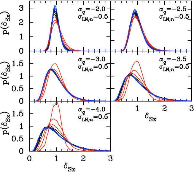
Figure 3: The probability distribution of the ensemble-averaged distribution of $\delta_{\mathrm{Sx}}$ illustrating the radial dependence. The distributions in shells of thickness $0.5\,r_{\mathrm{c}}$ are shown. Each color indicates a different radial interval: $R<1.5\,r_{\mathrm{c}}$ (red), $1.5\,r_{\mathrm{c}}<R<3.5\,r_{\mathrm{c}}$ (black), and $R>3.5\,r_{\mathrm{c}}$ (blue).

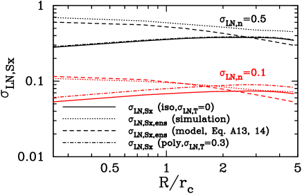
Figure 4: The radial dependence of the standard deviations of the logarithm of X-ray surface brightness, $\sigma_{\mathrm{LN},\,\mathrm{Sx}}$. Two values of $\sigma_{\mathrm{LN},\,n}$ are plotted, 0.1 and 0.5, as indicated in the figure. Solid and dotted lines show $\sigma_{\mathrm{LN},\,\mathrm{Sx}}(R)$ calculated using the average profile defined by the $\beta$ model (Eq. [11]) and the ensemble average (Eq. [13]), respectively. Dashed lines show the analytical prediction (Eq. [A18]) . Dash-dotted lines indicate the case including the temperature structure. Although we show results only for a single power-law index, $\alpha_{q}=-3.0$, similar results are obtained in other cases.

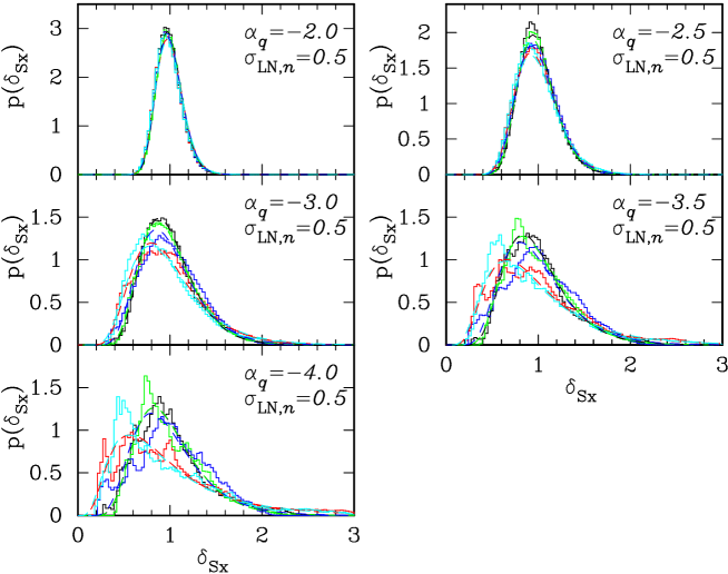
Figure 5: The probability distribution of $\delta_{\mathrm{Sx}}$ for five individual synthetic clusters (solid) along with the best-fit lognormal distributions (dashed). Each color shows a different individual synthetic cluster. Each panel shows a different value of the power law index of the Gaussian field, $\alpha_{q}$, between $-2$ and $-4$ as indicated in each panel.

We investigate the distribution of $\delta_{\mathrm{Sx}}$ as a function of radial distance $R$ from the cluster center. We first divide the $\delta_{\mathrm{Sx}}$ field into shells of thickness $0.5\,r_{\mathrm{c}}$. The distributions of $\delta_{\mathrm{Sx}}$ within each shell, $p(\mbox{$\delta_{\mathrm{Sx}}$};R)$, averaged over 256 synthetic clusters are shown in Figure 3 for various values of $\alpha_{q}$. We find that $\delta_{\mathrm{Sx}}$ also approximately follows the lognormal distribution. The standard deviation of the logarithm of $\delta_{\mathrm{Sx}}$ versus radius, $\sigma_{\mathrm{LN},\,\mathrm{Sx}}(R)$, constructed from the averaged shells is displayed in Figure 4. Two values of $\sigma_{\mathrm{LN},\,n}$ are plotted, 0.1 and 0.5, in addition to using the average profile defined by both the $\beta$ model (Eq. [11]; solid) and that for the ensemble (Eq. [13]; dotted). The analytic prediction (Eq. [A18]; dashed) and the case including the temperature structure (§3.3.2; dot-dashed) are also plotted. At large $R$, $\sigma_{\mathrm{LN},\,\mathrm{Sx,ens}}(R)$ is approximately $\sigma_{\mathrm{LN},\,\mathrm{Sx}}(R)$ because the spatial average tends to the ensemble average due to the large volume used for averaging. However, the agreement is poor near the center, where the ensemble average is not a good approximation. Although only one value for $\alpha_{q}$ is shown, similar results are obtained for other values.

Figures  3 and 4 indicate that the probability density function is weakly dependent on the projected radius $R$. This radial dependence is caused mainly by two competing effects. Consider first the case where the typical nonlinear scale of fluctuations is much smaller than the size of the cluster itself (shallow spectrum). As equation (A1) indicates, the surface brightness at $R$ is given by

$$S_{\mathrm{X}}(R)\propto\int\delta_{nn}\left[1+\left(\frac{l^{2}}{r_{\mathrm{c}}^{2}+R^{2}}\right)\right]^{-3\beta}dl.$$ (15)

This implies that the mean value of $S_{\mathrm{X}}(R)$ is effectively determined by the integration over the line of sight weighted towards the cluster center, roughly between $-\sqrt{r_{\mathrm{c}}^{2}+R^{2}}$ and $+\sqrt{r_{\mathrm{c}}^{2}+R^{2}}$. This is also true for the variance of $S_{\mathrm{X}}(R)$. Since the effective number of independent cells contributing to the variance of $S_{\mathrm{X}}(R)$ is smaller at smaller projected radii, $\sigma_{\mathrm{LN},\,\mathrm{Sx}}$ slightly increases for smaller $R$. This explains the behavior of the shallow spectra results for $\alpha_{q}=-2$ and $-2.5$ in Figure 3. On the contrary, if the typical nonlinear scale of fluctuations is comparable to or even larger than the cluster size (steep spectrum), the sampling at the central region significantly underestimates the real variance. So the $\sigma_{\mathrm{LN},\,\mathrm{Sx}}$ should increase toward the outer region. This is seen in Figure 3 for the steeper spectra, $\alpha_{q}=-3.5$ and $-4$.

Note the first effect is very small and the second effect becomes significant only when $\alpha_{q}<-3$. The cosmological hydrodynamic simulations imply that the typical value of $\alpha_{q}$ is $-3$. Therefore we neglect the radial dependence of the $\delta_{\mathrm{Sx}}$ field in the following analysis.

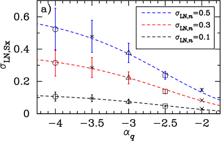
Figure 6: The average of $\sigma_{\mathrm{LN},\,\mathrm{Sx}}$ from the 256 synthetic cluster sample as functions of $\alpha_{q}$ (left) and $\sigma_{\mathrm{LN},\,n}$ (right). The left panel also shows the standard deviation of $\sigma_{\mathrm{LN},\,\mathrm{Sx}}$ from the 256 synthetic clusters and black, red, and blue represent different values of $\sigma_{\mathrm{LN},\,n}$, $0.1$, $0.3$, and $0.5$, respectively. In both panels, symbols indicate values of $\alpha_{q}$ (cross, square, triangle, asterisk, and circle correspond to $\alpha_{q}=-2$, $-2.5$, $-3$, $-3.5$, and $-4$, respectively). Dashed lines show the best-fit approximately linear $\sigma_{\mathrm{LN},\,\mathrm{Sx}}$-$\sigma_{\mathrm{LN},\,n}$ relation (Eq. 16 and Eq.  17) for each pair of $\sigma_{\mathrm{LN},\,n}$, $\alpha_{q}$.

From actual observations, we obtain the $\delta_{\mathrm{Sx}}$ map for an individual cluster, not the ensemble average. Therefore, we evaluate the distributions of $\delta_{\mathrm{Sx}}$ in individual synthetic clusters. Figure 5 shows the PDF for five individual synthetic clusters (solid) along with the best-fit lognormal distributions (dashed). We neglect the radial dependence and use the distribution for the whole cluster within a diameter of $L_{\mathrm{box}}=10\,r_{\mathrm{c}}$. Each color represents a different individual synthetic cluster and each panel shows a different value of the power-law index of the Gaussian field, $\alpha_{q}$, with values between -2 and -4. Even if the analysis is done for one cluster, the distribution approximately follows the lognormal distribution.

The noisy behavior for steeper spectra ($\alpha_{q}=-3.5$, $-4$) in Figure 5 is due to the presence of fluctuations on scales larger than that of the cluster, similar to the discussion above for Figure 3. In other words, steeper spectra ($\alpha_{q}<-3$) have relatively more larger scale fluctuations compared to shallower spectra ($\alpha_{q}>-3$). Cosmological hydrodynamic simulations suggest that $\alpha_{q}\approx 3$, placing galaxy clusters in the less noisy regime. We do not consider the noisy regime further in this paper.

The standard deviations of the logarithm of $\delta_{\mathrm{Sx}}$, $\sigma_{\mathrm{LN},\,\mathrm{Sx}}$, for the different sets of $\alpha_{q}$ (symbols) and $\sigma_{\mathrm{LN},\,n}$ (colors) are shown in Figure 6. The relation between $\sigma_{\mathrm{LN},\,n}$ and $\sigma_{\mathrm{LN},\,\mathrm{Sx}}$ is approximately linear (right panel) although the proportionality coefficient depends on $\alpha_{q}$. Therefore, we can write

$$\sigma_{\mathrm{LN},\,\mathrm{Sx}}=Q(\alpha_{q})\sigma_{\mathrm{LN},\,n}.$$ (16)

We find that $Q(\alpha_{q})$ can be approximated well by the following function

$$Q(\alpha_{q})=\frac{c_{1}}{c_{2}+|\alpha_{q}|^{-4}}.$$ (17)

We calculate the average of $\sigma_{\mathrm{LN},\,\mathrm{Sx}}/\sigma_{\mathrm{LN},\,n}$ for each $\alpha_{q}$ over three different values of $\sigma_{\mathrm{LN},\,n}$ ($\sigma_{\mathrm{LN},\,n}=0.1,0.3,$ and $0.5$). By fitting $\sigma_{\mathrm{LN},\,\mathrm{Sx}}/\sigma_{\mathrm{LN},\,n}(\alpha_{q})$ using equation (17), we obtain $c_{1}=2.05\times 10^{-2}$ and $c_{2}=1.53\times 10^{-2}$.

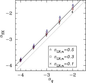
Figure 7: Comparison of the X-ray surface brightness ($\alpha_{\mathrm{Sx}}$) and the input Gaussian field ($\alpha_{q}$) power-law indices. Symbols and error bars indicate the average and the standard deviation, respectively, of $\alpha_{\mathrm{Sx}}$ for 256 samples for different sets of $\alpha_{q}$ and $\sigma_{\mathrm{LN},\,n}$. Symbols correspond to different values of $\sigma_{\mathrm{LN},\,n}$, with cross, square, and triangle symbols indicating $\sigma_{\mathrm{LN},\,n}=0.1$, $0.3$, and $0.5$, respectively, and the relations $\alpha_{\mathrm{Sx}}=\alpha_{q}$ and $\alpha_{\mathrm{Sx}}=\alpha_{q}+0.2$ are also shown (dotted and solid lines, respectively). We obtain $\alpha_{\mathrm{Sx}}$ for each individual synthetic cluster by fitting $P_{S_{\mathrm{X}}}({\bf K})$ of an individual cluster under the assumption of both statistical isotropy and a power-law ($\propto K^{\alpha_{\mathrm{Sx}}}$).

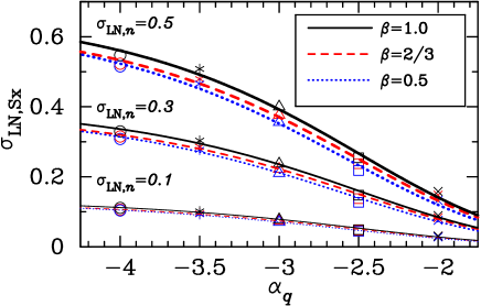
Figure 8: The average of $\sigma_{\mathrm{LN},\,\mathrm{Sx}}$ over the 256 synthetic clusters as a function of $\alpha_{q}$ for different values of the $\beta$ model power-law index, $\beta$. Symbols correspond to different values of $\alpha_{q}$ as in Figure 6. Each color shows a different value of $\beta$ (black, red, and blue correspond to $\beta=1.0,2/3,$ and $0.5$, respectively). Solid, dashed, and dotted lines are fits using equation (16), corresponding to $\beta=1.0,2/3,$ and $0.5$, respectively. The top, middle, and bottom sets of three different lines indicate $\sigma_{\mathrm{LN},\,n}=0.5,0.3$, and $0.1$, respectively, as indicated in the figure.

3.2.2 Spectral Considerations

Because $\sigma_{\mathrm{LN},\,\mathrm{Sx}}$ is strongly dependent on the power-law index $\alpha_{q}$, the estimate of $\alpha_{q}$ from the $\delta_{\mathrm{Sx}}$ map is crucial for interpreting the value of $\sigma_{\mathrm{LN},\,\mathrm{Sx}}$. Because $\alpha_{q}$ is an un-observable quantity, we investigate the relationship between the power spectra of $\delta_{n}$ and $\delta_{\mathrm{Sx}}$ by fitting the power spectrum of $\delta_{\mathrm{Sx}}$ under the assumptions of both statistical isotropy and a power law so that $P_{S_{\mathrm{X}}}({\bf K})\propto K^{\alpha_{\mathrm{Sx}}}$, where ${\bf K}$ indicates the two-dimensional wave vector.

Figure 7 shows the power-law index of the X-ray surface brightness, $\alpha_{\mathrm{Sx}}$, as a function of its counterpart Gaussian field, $\alpha_{q}$. Averages and standard deviations over 256 synthetic clusters are shown for three values of the standard deviation of the logarithm of density, $\sigma_{\mathrm{LN},\,n}$, where crosses, squares, and triangles correspond to $\sigma_{\mathrm{LN},\,n}$ of $0.1$, $0.3$, and $0.5$, respectively. The dotted line corresponds to the relation $\alpha_{\mathrm{Sx}}=\alpha_{q}$ and the solid line shows $\alpha_{\mathrm{Sx}}=\alpha_{q}+0.2$. We find that $\alpha_{\mathrm{Sx}}\approx\alpha_{q}+0.2$ and since $\alpha_{q}\approx\alpha_{n}$, this implies $\alpha_{\mathrm{Sx}}\approx\alpha_{n}+0.2$. This can be understood as follows. As we have seen in § 3.1, the difference between $\alpha_{n}$ and $\alpha_{nn}$ is relatively small ($\lesssim 13$% and often $\lesssim 5$%). If one assumes $\delta_{\mathrm{Sx}}$ is the projection of $\delta_{nn}$ (although this is only strictly true if the average of the surface brightness is defined by the ensemble average as Eq.[12]), $\delta_{\mathrm{Sx}}$ can be described as

$$\mbox{$\delta_{\mathrm{Sx}}$}({\bf\Theta})=\int dl\,\delta_{nn}\,W({\bf\Theta},l),$$ (18)

where ${\bf\Theta}$ indicates celestial coordinates and $W({\bf\Theta},l)$ is the window function. If we neglect the ${\bf\Theta}$-dependence of the window function and set $W({\bf\Theta},l)=W(l)$, then $P_{S_{\mathrm{X}}}({\bf K})$ can be written as

$$P_{S_{\mathrm{X}}}({\bf K})=\frac{1}{2\pi}\int dk_{l}\,P_{nn}({\bf k})\,|\widetilde{W}(k_{l})|^{2},$$ (19)

where $\widetilde{W}(k_{l})$ is the Fourier transform of $W(l)$. The assumption that the size of the cluster is much larger than the typical scales of the fluctuations yields $|\widetilde{W}(k_{l})|^{2}\sim 2\pi\delta(k_{l})$, where $\delta(k_{l})$ is the Dirac delta function, and therefore $K^{\alpha_{\mathrm{Sx}}}\propto k^{\alpha_{nn}}$. Thus, we find $\alpha_{n}\sim\alpha_{nn}\sim\alpha_{\mathrm{Sx}}$ ($\sim\alpha_{q}$).

In this section, we have found that, in principle, one can estimate the value of $\sigma_{\mathrm{LN},\,n}$ from analysis of X-ray observations. From the observations one measures $\sigma_{\mathrm{LN},\,\mathrm{Sx}}$ and $\alpha_{\mathrm{Sx}}$ and uses them to infer $\sigma_{\mathrm{LN},\,n}$, noting that $\alpha_{q}=\alpha_{\mathrm{Sx}}-0.2$. Therefore, one can estimate the statistical nature of the intrinsic three dimensional fluctuations from two dimensional X-ray observations.

3.3 Potential Systematics

Using mock observations of isothermal $\beta$ models we found a relation between the intrinsic inhomogeneity of the three dimensional cluster gas and the fluctuations in the X-ray surface brightness. We turn our attention to the effects of departures from this idealized model.

3.3.1 $\beta$ Model Power-law Index

In the above description, we have fiducially assumed the $\beta$ model power-law index $\beta=2/3$. We investigate two other cases, $\beta=0.5$, and $\beta=1.0$, in Figure 8, where we show $\sigma_{\mathrm{LN},\,\mathrm{Sx}}$ as a function of $\alpha_{q}$ for different cases of $\beta$ (colors). The corresponding fits using equation (16) are also shown. Although $\sigma_{\mathrm{LN},\,\mathrm{Sx}}$ tends to increase with increasing $\beta$, the change is relatively small ($<10$%).

3.3.2 Temperature Structure

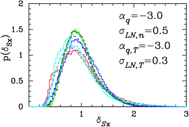
Figure 9: The distribution of $\delta_{\mathrm{Sx}}$ for five individual clusters including the effects of temperature structure. Synthetic clusters (solid histogram) and best-fit lognormal model (dashed lines) are both shown for each cluster. Each color corresponds to a different individual synthetic cluster. Although we display only one example of the power-law index, $\alpha_{q}=-3.0$, similar results are also obtained in other cases.

In the above discussion, we assumed isothermality for the ICM. However, the X-ray surface brightness also depends on the underlying cluster temperature structure, including a non-isothermal average temperature profile and local inhomogeneity. We investigate these effects for the X-ray surface brightness distribution.

We assume a polytropic profile for the temperature radial distribution expressed as

$$\overline{T}(r)=T_{0}\left(\frac{\overline{n}(r)}{n_{0}}\right)^{\gamma-1},$$ (20)

with polytropic index $\gamma=1.2$ and $T_{0}=6$ keV, which is the typical set of values in simulated clusters (Paper I). The ensemble average of the power spectrum of $\delta_{T}$ is assumed to have a power-law form ($\langle P_{T}(k)\rangle\sim P_{q}(k)\propto k^{\alpha_{q,T}}$). Because $\alpha_{T}\approx\alpha_{q,T}$ for the same reasons as described in § 3.1 for density fluctuations, we fiducially adopt the power-law index $\alpha_{q,T}=-3$ based on the results of cosmological hydrodynamic simulations (for details see § 2.2).

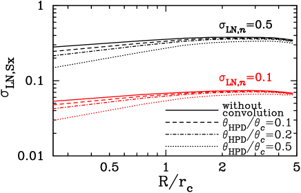
Figure 10: The effect of the PSF on $\sigma_{\mathrm{LN},\,\mathrm{Sx}}$ as a function of radius, $R/r_{\mathrm{c}}$, for the case of $\alpha_{q}=-3$ and $\beta=2/3$. Solid curves show $\sigma_{\mathrm{LN},\,\mathrm{Sx}}(R)$ without convolution of the PSF. Dashed, dash-dotted, and dotted curves correspond to $\theta_{\mathrm{HPD}}/\theta_{\mathrm{c}}=0.1,0.2$ and $0.5$, respectively. Two values of $\sigma_{\mathrm{LN},\,n}$ are plotted, 0.1 and 0.5, as indicated in the figure.

We create the lognormal distribution $\delta_{T}$ for temperature fluctuations in the same manner as for the density fluctuations described in § 3.1. The temperature of an arbitrary point is assigned according to

$$T({\bf r})=\delta_{T}({\bf r})\overline{T}(r).$$ (21)

We adopt $\sigma_{\mathrm{LN},\,T}=0.3$, because it is the typical value for simulated clusters (Paper I). In addition, we assume that $\delta_{n}$ and $\delta_{T}$ are distributed independently, following Paper I. The X-ray surface brightness is given by

$$S_{\mathrm{X}}({\bf R})\;\propto\int[n({\bf r})]^{2}\,\Lambda[T({\bf r})]\,dl,$$ (22)

where $\Lambda(T)$ is the X-ray cooling function. We calculate $\Lambda(T)$ in the energy range 0.5-10.0 keV using SPEX 2.0 (Kaastra et al., 1996) on the assumption of collisional ionization equilibrium and a constant metallicity of 30% solar abundances.

Examples of the distribution of $\delta_{\mathrm{Sx}}$ in individual clusters are shown in Figure 9 (solid histogram) along with the best fit lognormal distributions (dashed lines). Each color corresponds to a different individual synthetic cluster. Although only one value for the power-law index, $\alpha_{q}=-3$, is shown, similar results are obtained for other values. The radial dependence of $\sigma_{\mathrm{LN},\,\mathrm{Sx}}$ including the effects of temperature structure is shown in Figure 4 (dot-dashed).

There are only small differences between the isothermal and non-isothermal cases. The X-ray surface brightness depends on the density squared but roughly as $\sqrt{T}$ for bremsstrahlung emission. Therefore, the temperature structure effects on $\delta_{\mathrm{Sx}}$ are much less important than those of the density structure. Hereafter, we neglect the effects of temperature structure and focus only on the effects of density inhomogeneity.

3.3.3 Finite Spatial Resolution

Actual observations by X-ray satellites have finite spatial resolution, characterized by the point spread function (PSF). We assume that the PSF is a circularly symmetric Gaussian with standard deviation $\sigma$. The PSF can then be parameterized by a single parameter called the half power diameter ($\theta_{\mathrm{HPD}}$) in which 50% of the X-rays are enclosed ($\theta_{\mathrm{HPD}}/\sigma=2\sqrt{2\log 2}$). We investigate three cases, $\theta_{\mathrm{HPD}}/\theta_{\mathrm{c}}=0.1,0.2$ and $0.5$. Figure 10 shows the effect of the PSF on $\sigma_{\mathrm{LN},\,\mathrm{Sx}}$ as a function of radius. In each case, the average over 256 synthetic clusters is shown. Results for no PSF correction ($\theta_{\mathrm{HPD}}=0$, solid) and $\theta_{\mathrm{HPD}}/\theta_{\mathrm{c}}=0.1$ (dashed), 0.2 (dot-dashed), and 0.5 (dotted) are shown. As $\theta_{\mathrm{HPD}}/\theta_{\mathrm{c}}$ increases, $\sigma_{\mathrm{LN},\,\mathrm{Sx}}$ near the center of the cluster decreases. This can be understood as follows. In each radial shell, fluctuations smaller than roughly the radius of the shell predominately contribute to the fluctuations, namely $\sigma_{\mathrm{LN},\,\mathrm{Sx}}(R)$. The PSF effectively smooths out the smaller scale fluctuations (roughly up to the size of the PSF), reducing $\sigma_{\mathrm{LN},\,\mathrm{Sx}}$, while preserving the large scale fluctuations. Since the inner shells only contain small scale fluctuations, they are more strongly affected by the PSF. The case of $\theta_{\mathrm{HPD}}/\theta_{\mathrm{c}}=0.5$ best illustrates these effects. The reduction of $\sigma_{\mathrm{LN},\,\mathrm{Sx}}$ from the PSF is seen at all radii. However, it is only a slight reduction at large radii, increasing as the radius decreases, with a very large effect near the cluster center.

In summary, when $\delta_{n}$ in three dimensions follows the lognormal distribution, $\delta_{\mathrm{Sx}}$ in two dimensions also approximately follows the lognormal distribution. The mean value of $\sigma_{\mathrm{LN},\,\mathrm{Sx}}$ for an individual cluster is strongly dependent on both $\sigma_{\mathrm{LN},\,n}$ and $\alpha_{q}$. Because $\alpha_{q}$ is approximately equal to $\alpha_{\mathrm{Sx}}$, in principle, one can infer $\sigma_{\mathrm{LN},\,n}$ from $\sigma_{\mathrm{LN},\,\mathrm{Sx}}$ although there is still some dispersion even if $\alpha_{q}$ is known. In addition, the effect of the temperature structure is minimal.

4 Application to Abell 3667

Simulations suggest that the lognormal model (Eq. [3]) is a reasonable approximation of the small scale structure in galaxy clusters. We compare this model with Chandra X-ray observations of the nearby galaxy cluster Abell 3667 at a redshift $z=0.056$ (Struble, M. F., & Rood, J. H, 1999). A3667 is a well observed nearby bright galaxy cluster that does not exhibit a cool core observed by Chandra . With its complex structure, including a cold front (Vikhlinin, Markevitch, & Murray, 2001) and possible merger scenario (e.g., Knopp, Henry, & Briel, 1996), A3667 will serve as a difficult test case for the lognormal model of density fluctuations.

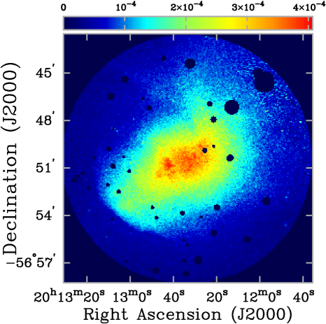
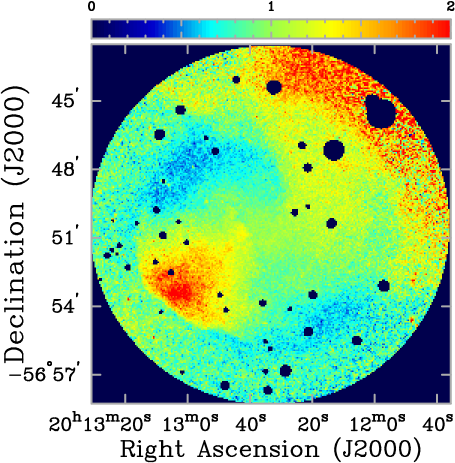
Figure 11: Chandra image of the galaxy cluster Abell 3667 (left) and the corresponding $\delta_{\mathrm{Sx}}$ image (right). The counts image has been divided by the exposure map to yield X-ray surface brightness (cnt s^-1 cm^-2 arcmin^-2), including scaling for the pixel size. Point sources in the field have been masked.

Table 1: A3667 Chandra Observations

	$t_{exp}$	RA	DEC
obsID	(ks)	(h m s)	(d m s)
$\phantom{0}513$	$\phantom{0}45$	$20\ 12\ 50.30$	$-56\ 50\ 56.99$
$\phantom{0}889$	$\phantom{0}51$	$20\ 11\ 50.00$	$-56\ 45\ 34.00$
$5751$	$131$	$20\ 13\ 07.25$	$-56\ 53\ 24.00$
$5752$	$\phantom{0}61$	$20\ 13\ 07.25$	$-56\ 53\ 24.00$
$5753$	$105$	$20\ 13\ 07.25$	$-56\ 53\ 24.00$
$6292$	$\phantom{0}47$	$20\ 13\ 07.25$	$-56\ 53\ 24.00$
$6295$	$\phantom{0}50$	$20\ 13\ 07.25$	$-56\ 53\ 24.00$
$6296$	$\phantom{0}50$	$20\ 13\ 07.25$	$-56\ 53\ 24.00$

4.1 Data Reduction

Chandra observations of the galaxy cluster A3667 are summarized in Table 1. Listed are the observation identification numbers, exposure times, and pointing centers of each of the eight archival Chandra observations of A3667 used in this analysis. The data are reduced with CIAO version 4.0 and calibration data base version 3.4.2. The data are processed starting with the level 1 events data, removing cosmic ray afterglows, correcting for charge transfer inefficiency and optical blocking filter contamination, and other standard corrections, in addition to generating a customized bad pixel file. The data are filtered for ASCA grades 0, 2, 3, 4, 6 and status=0 events and the good time interval data provided with the observations are applied. Periods of high background count rate are excised using an iterative procedure involving creating light curves in background regions with 500 s bins, and excising time intervals that are in excess of 4 $\sigma$ from the median background count rate. This sigma clipping procedure is iterated until all remaining data lie within 4 $\sigma$ of the median. The final events list is limited to energies 0.7-7.0 keV to exclude the low and high energy data that are more strongly affected by calibration uncertainties. Finally, the images are binned by a factor of eight, resulting in a pixel size of 3.94″. This pixel size matches the resolution of the synthetic clusters considered in §3. In particular, the ratio of pixel size to the cluster core radius of the Chandra image is similar to the synthetic cluster grid spacing compared to the synthetic cluster core radius, namely, for $\theta_{\mathrm{c}}\sim 180\arcsec$ (Reiprich & Böhringer, 2002; Knopp, Henry, & Briel, 1996), $\theta_{\mathrm{pix}}/\theta_{\mathrm{c}}\sim d_{\mathrm{grid}}/r_{\mathrm{c}}\sim 0.02$. Exposure maps are constructed for each observation at an energy of 1 keV. The binned images and exposure maps for each observation are then combined to make the single image and exposure map used for the analysis.

A wavelet based source detector is used to find and generate a list of potential point sources. The list is examined by eye, removing bogus or suspect detections, and then used as the basis for our point source mask. Figure 11 (left) shows the Chandra merged image of A3667, the counts image divided by the exposure map, where the point source mask has been applied. Also shown is the $\delta_{\mathrm{Sx}}$ image (right), discussed below. A cold front (Vikhlinin, Markevitch, & Murray, 2001) is clearly visible in the south-eastern region of the $\delta_{\mathrm{Sx}}$ image.

4.2 Analysis and Results

In order to determine the center of A3667, a $\beta$ model is fit to the data with fixed core radius ($180\arcsec$) and $\beta$ (2/3), using software originally developed for the combined analysis of X-ray and Sunyaev-Zel’dovich effect observations (Reese et al., 2000, 2002; Bonamente et al., 2006). Because A3667 is nearby and appears very large, Chandra observations do not encompass the entire cluster but provide a wealth of information on the complexities inherent in galaxy cluster gas. By using a $\beta$ model fit to the diffuse emission of the cluster gas we obtain a better measurement of its center than simply using the brightest pixel or other simple estimates, which fail to take into account the complex structure manifest in this cluster. A circular region of radius $\sim 8\arcmin$ centered on A3667 is used in the analysis, corresponding to two and a half times the cluster’s core radius, the largest usable region from the arrangement of the combined Chandra observations.

The average X-ray surface brightness is required to compute $\mbox{$\delta_{\mathrm{Sx}}$}=S_{\mathrm{X}}/\overline{S}_{\mathrm{X}}$. If one computes the average surface brightness, $\overline{S}_{\mathrm{X}}$, in annular shells, then one will tend to under (over) estimate $\overline{S}_{\mathrm{X}}$ toward the inner (outer) radius of each annulus. Therefore, this will lead to an over (under) estimate of $\delta_{\mathrm{Sx}}$ toward the inner (outer) radius of each annulus. To alleviate this systematic, we adopt the azimuthally averaged X-ray surface brightness as the model for $\overline{S}_{\mathrm{X}}$, and use cubic spline interpolation between radial bins. The X-ray surface brightness radial profile for A3667 is shown in Figure 12, along with the interpolated model (line).

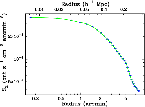
Figure 12: Chandra radial profile of the galaxy cluster Abell 3667 (points) with the interpolated model (solid line). This model is used as the average X-ray surface brightness distribution in the calculation of $\delta_{\mathrm{Sx}}$.

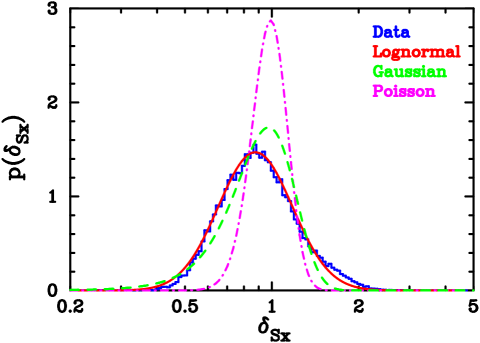
Figure 13: Probability distribution of $\delta_{\mathrm{Sx}}$ from Chandra observations of the galaxy cluster Abell 3667 (blue histogram) along with the best fit lognormal distribution (red line) with $\sigma_{\mathrm{LN},\,\mathrm{Sx}}=0.30$. The lognormal distribution seems to be a reasonable description of the ICM inhomogeneity in A3667. Also shown are the best-fit Gaussian model (dashed green) and a Poisson model (dot-dashed magenta) using the average counts per pixel within the fitting region.

Figure 14: Power spectrum of $\delta_{\mathrm{Sx}}$ (thick solid) from Chandra observations of the galaxy cluster Abell 3667, normalized to one at the largest scale. Also plotted are three power-law power spectra with spectral indices of -2 (dashed), -3 (dot-dashed), and -4 (dotted) for comparison.

The probability distribution of $\delta_{\mathrm{Sx}}$, $p(\mbox{$\delta_{\mathrm{Sx}}$})$, is computed from the histogram of pixels calculated from the $\delta_{\mathrm{Sx}}$ image and shown in Figure 13. The lognormal distribution (Eq. [3]) is fit to the $p(\mbox{$\delta_{\mathrm{Sx}}$})$ of A3667, where the only free parameter is the standard deviation of the logarithm of $\delta_{\mathrm{Sx}}$, $\sigma_{\mathrm{LN},\,\mathrm{Sx}}$. The best fit value for the lognormal model is $\sigma_{\mathrm{LN},\,\mathrm{Sx}}=0.30$. In addition, a Gaussian distribution is also fit to the data, with its usual two parameters, the mean and standard deviation. Figure 13 shows the PDF of $\delta_{\mathrm{Sx}}$ for the Chandra observations of the galaxy cluster A3667 (solid blue histogram). The best fit lognormal (solid red) and Gaussian (dashed green) models are also shown. A Poisson distribution (dot-dashed magenta) is also shown for comparison, using the average counts per pixel in the fitting region as the parameter for the Poisson distribution. Clearly, what is seen is not the result of Poisson statistics. The lognormal model seems to be a reasonable match to the observed PDF.

However, without information on the power spectrum of the $\delta_{\mathrm{Sx}}$ fluctuations, it is difficult to interpret the value of $\sigma_{\mathrm{LN},\,\mathrm{Sx}}$ (§3.2.2) and relate it to the fluctuations in the density distribution (Eqs. [16, 17]; Fig. 6). Therefore, we take the Fourier transform of the $\delta_{\mathrm{Sx}}$ image and compute the average power spectrum in wavenumber annuli. The power spectrum of $\delta_{\mathrm{Sx}}$ fluctuations is shown in Figure 14 (thick solid) along with three power-law spectra with spectral indices of -2 (dashed), -3 (dot-dashed), and -4 (dotted) for comparison. The power spectrum of $\delta_{\mathrm{Sx}}$ has been normalized to one at the largest scales. A simple power-law model fit to the power spectrum yields a spectral index of $\alpha_{\mathrm{Sx}}=-2.7$ using the entire spectrum, and a spectral index of $\alpha_{\mathrm{Sx}}=-3.0$ if excluding the larger wavenumbers ($\gtrsim 2$ arcmin^-1), roughly where the power spectrum changes shape.

4.3 Implications

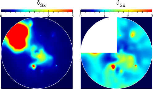
Figure 15: An example of a $\delta_{\mathrm{Sx}}$ map from a cosmological hydrodynamic simulated cluster (“Centaurus”) both before (left) and after (right) removal of a quadrant with a large clump. Circles show the projected virial radius ($R_{\mathrm{200}}$). Although within the projected virial radius, $R_{\mathrm{200}}$, these structures often reside outside of the three-dimensional virial radius, $r_{\mathrm{200}}$.

Both the standard deviation of the logarithm of X-ray surface brightness fluctuations, $\sigma_{\mathrm{LN},\,\mathrm{Sx}}=0.30$, and the power spectrum power-law index $\alpha_{\mathrm{Sx}}\approx-3$, fall into the range expected from hydrodynamical galaxy clusters and therefore used in the synthesized cluster analysis (§2.2). By combining these pieces of information, we can relate the information obtained from the X-ray surface brightness distribution to that of the underlying density distribution, using the results of the synthesized cluster analysis. Using the synthetic cluster result that the spectral indices of the X-ray surface brightness fluctuations and that of the Gaussian field are simply related by $\alpha_{\mathrm{Sx}}\approx\alpha_{q}+0.2$, and the relation between $\sigma_{\mathrm{LN},\,n}$, $\sigma_{\mathrm{LN},\,\mathrm{Sx}}$, and $\alpha_{q}$ (Eqs. [16, 17]; Fig. 6), the Chandra results of $\sigma_{\mathrm{LN},\,\mathrm{Sx}}=0.30$ and $\alpha_{\mathrm{Sx}}=-2.7$ imply that the fluctuations in the underlying density distribution have $\sigma_{\mathrm{LN},\,n}=0.43$. A value of $\alpha_{\mathrm{Sx}}=-3.0$ implies $\sigma_{\mathrm{LN},\,n}=0.36$. The difficult test case of the A3667 X-ray surface brightness seems to follow the lognormal distribution of density fluctuations, thus enabling an estimate of the statistical properties of the underlying ICM density fluctuations.

5 Application to the Cosmological Hydrodynamic Simulated Clusters

Results from cosmological hydrodynamic simulations motivated the lognormal model for ICM inhomogeneity. In §3, we found that synthetic clusters with lognormal fluctuations show a linear relation between $\sigma_{\mathrm{LN},\,\mathrm{Sx}}$ and $\sigma_{\mathrm{LN},\,n}$. We now return to clusters extracted from cosmological hydrodynamic simulations to further explore these results.

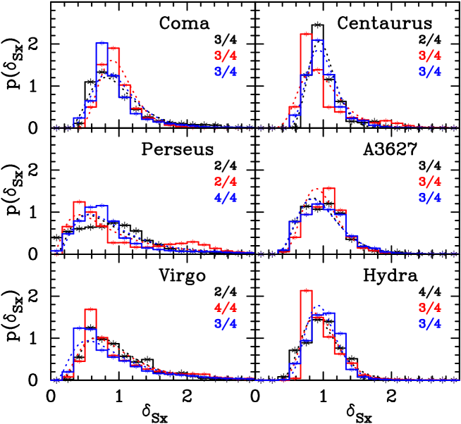
Figure 16: The distribution of $\delta_{\mathrm{Sx}}$ for each of the six clusters from a cosmological hydrodynamic simulation (points and solid histogram). Each color indicates the projection along a different, orthogonal line of sight. For each line of sight, we show the number of quadrants used for the analysis. For example, “3/4” indicates that one quadrant is excluded and three remain. The best fit lognormal model for each projection is also shown (dotted lines).

For each cluster extracted from the simulations, we create X-ray surface brightness maps towards three orthogonal directions, and compute $\mbox{$\delta_{\mathrm{Sx}}$}({\bf R})=S_{\mathrm{X}}({\bf R})/\overline{S}_{\mathrm{X}}(R)$ in a similar manner as described for the synthetic clusters in § 3.1.2. The regions we consider are within the projected virial radius $R_{\mathrm{2}00}$. The projected virial radius, $R_{\mathrm{200}}$, is the radius within which the mean interior density is 200 times that of the critical density.

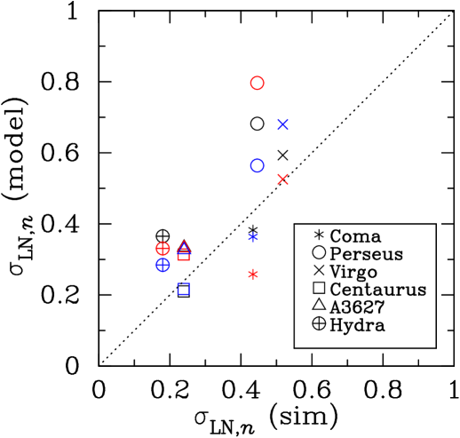
Figure 17: The density fluctuation standard deviation predicted by our model, $\sigma_{\mathrm{LN},\,n}(\mbox{model})=\sigma_{\mathrm{LN},\,\mathrm{Sx}}/Q(\alpha_{q})$ versus that from the simulations, $\sigma_{\mathrm{LN},\,n}(\mbox{sim})$. Symbols show different simulated clusters (see figure legend) and colors indicate different orthogonal lines of sight. Also plotted is the simple linear relation $\sigma_{\mathrm{LN},\,n}\mbox{(model)}=\sigma_{\mathrm{LN},\,n}\mbox{(sim)}$ for comparison.

Although the lognormal distribution is a good fit to the density (and temperature) of simulated galaxy clusters in three-dimensions, the projection to X-ray surface brightness suffers from the additional complexity of projection effects. If large clumps are present, the distribution of X-ray surface brightness fluctuations, $\delta_{\mathrm{Sx}}$, is not well approximated by the lognormal distribution. The large clumps artificially distort the average profile of the cluster and therefore bias the value of $\delta_{\mathrm{Sx}}$, which depends on the average profile. We also note that although these clumps fall within the projected virial radius, $R_{\mathrm{2}00}$, they usually fall outside of the three dimensional virial radius, $r_{\mathrm{2}00}$. We therefore exclude quadrants that contain large clumps, using $\mbox{$\delta_{\mathrm{Sx}}$}>10$ as the exclusion criterion. Then, we recompute $\overline{S}_{\mathrm{X}}(R)$ and $\delta_{\mathrm{Sx}}$. The complex structure of simulated clusters is illustrated in the $\delta_{\mathrm{Sx}}$ images shown in Figure 15, where examples of a simulated cluster both before and after removal of a quadrant are displayed. The circles show the projected virial radius, $R_{\mathrm{200}}$.

In Figure 16 the probability distributions of $\delta_{\mathrm{Sx}}$ for the simulated clusters (histograms) along with the best-fit lognormal model (dotted lines) are displayed. Each color indicates the projection along a different, orthogonal line of sight. Overall, the probability distributions of $\delta_{\mathrm{Sx}}$ are reasonably well approximated by the lognormal function, consistent with the results from the synthetic clusters (§ 3.2.1).

We now come full circle to compare our results from the synthetic clusters directly to the simulations. In order to do this, we look at the relationship between $\sigma_{\mathrm{LN},\,n}\mbox{(}\mathrm{sim})$ measured in the simulated clusters and $\sigma_{\mathrm{LN},\,n}\mbox{(}\mathrm{model})$ predicted from the synthetic cluster results, equations  (16) and (17), where we adopt $\alpha_{q}=\alpha_{\mathrm{Sx}}-0.2$ (see §3.2.2). The value of $\alpha_{\mathrm{Sx}}$ for each simulated cluster is obtained by fitting a power-law model, $P(K)\propto K^{\alpha_{\mathrm{Sx}}}$, to the power spectra of $\delta_{\mathrm{Sx}}$. Because the resolution of the simulations is much poorer than that of the synthetic clusters, we must recompute the coefficients $c_{1}$ and $c_{2}$ in equation 17 from a set of lower resolution synthetic clusters. Assuming $r_{\mathrm{c}}\sim 100$ $h^{-1}$ kpc for the simulated clusters, we choose the resolution $\sim 0.1d_{\mathrm{grid}}/r_{\mathrm{c}}$, noting that this value corresponds to the maximum resolution of the simulations. Performing the same procedure described in §3, we obtain $c_{1}=3.99\times 10^{-2}$ and $c_{2}=3.36\times 10^{-2}$.

We compare $\sigma_{\mathrm{LN},\,n}\mbox{(model)}$ and $\sigma_{\mathrm{LN},\,n}\mbox{(}\mathrm{sim})$ in Figure 17. Each color corresponds to a different line of sight. Although there is large scatter, these results indicate that it is possible to estimate $\sigma_{\mathrm{LN},\,n}$ within a factor of two only using the information obtained from the X-ray surface brightness distribution.

6 Summary

We have developed a method of extracting statistical information on the ICM inhomogeneity from X-ray observations of galaxy clusters. With a lognormal model for the fluctuations motivated by cosmological hydrodynamic simulations, we have created synthetic clusters, and have found that their X-ray surface brightness fluctuations retain the lognormal nature. In addition, the result that $\sigma_{\mathrm{LN},\,\mathrm{Sx}}$ and $\sigma_{\mathrm{LN},\,n}$ are linearly related implies that one can, in principle, estimate the statistical properties of the three dimensional density inhomogeneity ($\sigma_{\mathrm{LN},\,n}$) from X-ray observations of galaxy clusters ($\sigma_{\mathrm{LN},\,\mathrm{Sx}}$ and $\alpha_{\mathrm{Sx}}$).

We have compared the predictions of our model to Chandra X-ray observations of the galaxy cluster A3667. For the first time in a real galaxy cluster we were able to detect the lognormal signature of X-ray surface brightness fluctuations, which was originally motivated by simulations. Based on the synthetic cluster results, this enabled an estimate of the statistical properties of the inhomogeneity of the ICM of A3667. In the context of lognormally distributed inhomogeneity, we obtain $\sigma_{\mathrm{LN},\,n}\approx 0.4$ for the gas density fluctuations of A3667. It is encouraging that the value of the fluctuation amplitude for Abell 3667 is in reasonable agreement with typical values from the simulated clusters.

Finally we check the validity and limitation of our method using several clusters from cosmological hydrodynamic simulations. Unlike the fairly idealized synthetic clusters, simulated clusters exhibit complex structure more akin to real galaxy clusters. As a result, the empirical relation between the two- and three-dimensional fluctuation properties calibrated with synthetic clusters when applied to simulated clusters shows large scatter. Nevertheless we are able to reproduce the true value of the fluctuation amplitude of simulated clusters within a factor of two from their two-dimensional X-ray surface brightness alone.

Our current methodology combined with existing observational data is useful in describing and inferring the statistical properties of the three dimensional inhomogeneity in galaxy clusters. The fluctuations in the ICM have several implications in properly interpreting galaxy cluster data. In particular, our current model may be useful in interpreting data from current and future galaxy cluster surveys using the Sunyaev-Zel’dovich effect, which have the potential to provide tight constraints on cosmology.

Appendix A Relation of Density and Surface Brightness Distributions Under the Thick-slice Approximation

Modeling galaxy clusters with a spherical isothermal $\beta$ model (Eq. 11), the surface brightness at an arbitrary projected angular radius, $\theta$, is given by

$$S_{\mathrm{X}}(\theta) \propto \int_{-\infty}^{\infty}[n({\bf r})]^{2}dl$$ (A1)

$$= \int_{-\infty}^{\infty}\delta_{nn}({\bf r})\langle n^{2}\rangle(r=\sqrt{l^{2}+d_{A}^{2}\theta^{2}})dl$$

$$= M_{2}n_{0}^{2}\left(1+\frac{d_{A}^{2}\theta^{2}}{r_{c}^{2}}\right)^{-3\beta}\int_{-\infty}^{\infty}\delta_{nn}({\bf r})\left[1+\left(\frac{l}{r_{c,\mathrm{eff}}(\theta)}\right)^{2}\right]^{-3\beta}dl,$$

where $r_{c,\mathrm{eff}}(\theta)\equiv\sqrt{r_{c}^{2}+d_{A}^{2}\theta^{2}}$, and we assume the $\sigma_{{\rm LX},x}$ in equation 3 is independent of $r$. Therefore, the second moment of $n$ ($M_{2}\equiv\langle n^{2}\rangle/\langle n\rangle^{2}=\exp{(-\sigma_{\mathrm{LN},\,n}^{2})}$) is also independent of $r$. In the above, we use $\langle n\rangle=\overline{n}(r)$.

The ensemble average of $\langle S_{\mathrm{X}}(\theta)\rangle$ can be expressed as

$$\langle S_{\mathrm{X}}(\theta)\rangle \propto \int_{-\infty}^{\infty}\langle n^{2}\rangle(r=\sqrt{l^{2}+d_{A}^{2}\theta^{2}})dl$$ (A2)

$$= \sqrt{\pi}n_{0}^{2}M_{2}r_{c}\frac{\Gamma(3\beta-1/2)}{\Gamma(3\beta)}\left(1+\frac{d_{A}^{2}\theta^{2}}{r_{c}^{2}}\right)^{-3\beta+1/2}$$

Combining equations (A1) and (A2), $\delta_{\mathrm{Sx,ens}}$ reduces to

$$\delta_{\mathrm{Sx,ens}}(\theta) = \kappa_{\beta}\int_{-\infty}^{\infty}\delta_{nn}({\bf r})\left[1+\left(\frac{l}{r_{c,\mathrm{eff}}(\theta)}\right)^{2}\right]^{-3\beta}d\left(\frac{l}{r_{c,\mathrm{eff}}(\theta)}\right)$$

$$\kappa_{\beta} \equiv \pi^{-1/2}\frac{\Gamma(3\beta)}{\Gamma(3\beta-1/2)}.$$ (A3)

Now, fixing $\theta$, let us consider the three-dimensional field $\delta_{nn}({\bf r})W_{\beta}(l)$ and its projected two-dimensional field $\delta_{\mathrm{Sx,ens}}|_{\theta}$, defined as

$$\delta_{\mathrm{Sx,ens}}|_{\theta} = \int_{-\infty}^{\infty}\delta_{nn}({\bf r})W_{\beta}({l^{\prime}})d{l^{\prime}}$$ (A4)

$$W_{\beta}({l^{\prime}}) \equiv \kappa_{\beta}(1+{l^{\prime}}^{2})^{-3\beta},$$ (A5)

where we use a dimensionless length normalized by $r_{c,\mathrm{eff}}(\theta)$ distinguished by prime (${l^{\prime}}\equiv l/r_{c,\mathrm{eff}}(\theta)$, $k_{l}^{\prime}\equiv k_{l}r_{c,\mathrm{eff}}(\theta)$). Then, we can consider the variance of the $\delta_{\mathrm{Sx,ens}}|_{\theta}$-field,

$$\sigma_{\delta_{\mathrm{Sx,ens}}|_{\theta}}^{2}=\frac{1}{(2\pi)^{2}}\int d{\bf K^{\prime}}P_{S_{\mathrm{X,ens}}|_{\theta}}({\bf K^{\prime}}),$$ (A6)

where $P_{S_{\mathrm{X,ens}}|_{\theta}}({\bf K^{\prime}})$ is the (two-dimensional) power spectrum of $\delta_{\mathrm{Sx,ens}}|_{\theta}$. The variance of the $\delta_{nn}$ field can also be written as

$$\sigma_{\delta_{nn}}^{2}=\frac{1}{(2\pi)^{3}}\int d{\bf k^{\prime}}P_{nn}({\bf k^{\prime}}).$$ (A7)

With this, the relation between $P_{S_{\mathrm{X,ens}}}({\bf K^{\prime}})$ and $P_{nn}({\bf k^{\prime}})$ is

$$P_{S_{\mathrm{X,ens}}|_{\theta}}({\bf K^{\prime}})=\frac{1}{2\pi}\int dk_{l}^{\prime}P_{nn}({\bf k^{\prime}})|\widetilde{W}_{\beta}(k_{l}^{\prime})|^{2}.$$ (A8)

The Fourier conjugate $\widetilde{W}_{\beta}(k_{l}^{\prime})$ is given by

$$\widetilde{W}_{\beta}(k_{l}^{\prime})=\kappa_{\beta}\left(\frac{2}{k_{l}^{\prime}}\right)^{-3\beta+1/2}\frac{2\sqrt{\pi}}{\Gamma(3\beta)}K_{-3\beta+1/2}(k_{l}^{\prime}),$$ (A9)

where $K_{-3\beta+1/2}(k_{l}^{\prime})$ is modified Bessel function of the second kind .

In the case that the largest scale fluctuation is smaller than the physical scale (the thick-slice approximation, following Fischera & Dopita (2004)), the Fourier conjugate of the window function becomes the Dirac-delta function, $|\widetilde{W}_{\beta}(k_{l}^{\prime})|^{2}\sim g(\beta)\delta(k_{l}^{\prime})$. The normalization factor $g(\beta)$ is given by

$$g(\beta)\equiv 2\int_{0}^{\infty}dk_{l}^{\prime}|\widetilde{W}_{\beta}(k_{l}^{\prime})|^{2}=2\sqrt{\pi}\frac{\Gamma(3\beta)^{2}\Gamma(6\beta-1/2)}{\Gamma(3\beta-1/2)^{2}\Gamma(6\beta)}.$$ (A10)

Let us define the effective width

$$\Delta_{\mathrm{eff}}(\theta)\equiv 2\pi r_{c,\mathrm{eff}}(\theta)/g(\beta)=\sqrt{\pi}\frac{\Gamma(3\beta-1/2)^{2}\Gamma(6\beta)}{\Gamma(3\beta)^{2}\Gamma(6\beta-1/2)}r_{c,\mathrm{eff}}(\theta).$$ (A11)

Fischera & Dopita (2004) explore the column density distribution assuming a plane parallel geometry with width $\Delta$. In the thick slice case, $\Delta_{\mathrm{eff}}$ corresponds to $\Delta$ although they consider the column density not the surface brightness. We assume statistical isotropy and a power law spectrum with upper and lower limit ($k_{\mathrm{max}}^{\prime}\equiv k_{\mathrm{max}}r_{c,\mathrm{eff}}(\theta)$ and $k_{\mathrm{min}}^{\prime}\equiv k_{\mathrm{min}}r_{c,\mathrm{eff}}(\theta)$),

$$P_{nn}({\bf k^{\prime}})\left\{\begin{array}[]{lr}\propto|{\bf k^{\prime}}|^{\alpha_{nn}}&\mbox{$k_{\mathrm{min}}^{\prime}<|{\bf k^{\prime}}|<k_{\mathrm{max}}^{\prime}$}\\ =0&\mbox{otherwise.}\\ \end{array}\right.$$ (A14)

Finally, using equation (A6), (A7), and (A8) under the thick-slice approximation, we obtain

$$\sigma_{\delta_{\mathrm{Sx,ens}}|_{\theta}}^{2}/\sigma_{\delta_{nn}}^{2}=\left\{\begin{array}[]{lr}\displaystyle{\frac{1(\alpha_{nn}+3)(1-\zeta^{\alpha_{nn}+2})}{2(\alpha_{nn}+2)(1-\zeta^{\alpha_{nn}+3})}\left(\frac{\Delta_{\mathrm{eff}}(\theta)}{l_{\mathrm{max}}}\right)^{-1}}&\mbox{$\alpha_{nn}\neq-3$ and $\alpha_{nn}\neq-2$}\\ \displaystyle{\frac{\log\zeta}{2(\zeta-1)}\left(\frac{\Delta_{\mathrm{eff}}(\theta)}{l_{\mathrm{max}}}\right)^{-1}}&\mbox{$\alpha_{nn}=-2$}\\ \displaystyle{\frac{1-1/\zeta}{2\log\zeta}\left(\frac{\Delta_{\mathrm{eff}}(\theta)}{l_{\mathrm{max}}}\right)^{-1}}&\mbox{$\alpha_{nn}=-3$,}\\ \end{array}\right.$$ (A18)

where $\zeta\equiv k_{\mathrm{max}}/k_{\mathrm{min}}$ and $l_{\mathrm{max}}\equiv 2\pi k_{\mathrm{min}}^{-1}$.

Then, although $\sigma_{\delta_{\mathrm{Sx,ens}}|_{\theta}}^{2}$ is the variance of $\delta_{\mathrm{Sx,ens}}|_{\theta}$-field, we regard it as the variance of the ensemble average of $\delta_{\mathrm{Sx,ens}}({\bf R^{\prime}})$ at $\theta$. The conversion to the standard deviation of logarithm is expressed as

$$\sigma_{\mathrm{LN},\,\mathrm{Sx}}=\sqrt{\log{(1+\sigma_{\delta_{\mathrm{Sx,ens}}|_{\theta}}^{2})}}$$ (A19)

In Figure 4, we adopt $\zeta=L_{\mathrm{box}}/(2d_{\mathrm{grid}})=f_{\mathrm{s}}/f_{\mathrm{Ny}}$, where $f_{\mathrm{s}}$ and $f_{\mathrm{Ny}}$ are the sampling frequency and the Nyquist frequency, respectively, and $l_{\mathrm{max}}=L_{\mathrm{box}}$. We also adopt the fitted value of $\alpha_{nn}$ in equation (A18).

Appendix B Distribution of the Density Squared

If one assumes density inhomogeneity fluctuations, $\mbox{$\delta_{n}$}=n/\langle n\rangle$, follow the lognormal distribution, $p_{\mathrm{LN}}(\mbox{$\delta_{n}$};\sigma_{\mathrm{LN},\,n})$, the fluctuations of the density squared, $\delta_{nn}\equiv n^{2}/\langle n^{2}\rangle$ can be written as

$$\delta_{nn}=\mbox{$\delta_{n}$}^{2}\frac{\langle n\rangle^{2}}{\langle n^{2}\rangle}=\mbox{$\delta_{n}$}^{2}\exp{(-\sigma_{\mathrm{LN},\,n}^{2})}.$$ (B1)

where $\langle\,\rangle$ indicates ensemble average.

For simplicity, we replace $\delta_{n}$ and $\delta_{nn}$ by $x$ and $y$, respectively,

$$x\equiv\mbox{$\delta_{n}$};y\equiv\delta_{nn}.$$ (B2)

Therefore, the relation between $x$ and $y$ is

$$x=\sqrt{y}\exp{(\sigma_{\mathrm{LN},\,n}^{2}/2)}.$$ (B3)

Because $x$ follows $p_{\mathrm{LN}}(x;\sigma_{\mathrm{LN},\,n})$, the distribution of $y$ is obtained by

$$p(y)=p_{\mathrm{LN}}(x;\sigma_{\mathrm{LN},\,n})\frac{dx}{dy}=p_{\mathrm{LN}}(y;2\sigma_{\mathrm{LN},\,n}).$$ (B4)

Therefore, $\delta_{nn}$ follows the lognormal distribution with lognormal standard deviation of $2\sigma_{\mathrm{LN},\,n}$.

References

- Albrecht et al. (2006) Albrecht, A., et al., 2006, astro-ph/0609591
- Birkinshaw (1999) Birkinshaw, M., 1999, Phys. Rep., 310, 97
- Bradač et al. (2006) Bradač, M., Clowe, D., Gonzalez, A. H., Marshall, P., Forman, W., Jones, C., Markevitch, M., Randall, S., Schrabback, T., & Zaritsky, D., 2006, ApJ, 652, 937
- Bartlett & Silk (1994) Bartlett, J. G., Silk, J., 1994, ApJ, 423, 12
- Bonamente et al. (2006) Bonamente et al., 2006, ApJ, 647, 25
- Briel et al. (2004) Briel, U. G., Finoguenov, A., & Henry, J. P.2004, A&A 426,1
- Carlstrom et al. (2002) Carlstrom, J. E., Holder, G. P., and Reese, E. D. 2002, ARA&A, 40, 643
- Cavaliere & Fusco-Femiano (1976) Cavaliere, A. & Fusco-Femiano, R., 1976, A&A, 49, 137
- Cavaliere & Fusco-Femiano (1978) Cavaliere, A. & Fusco-Femiano, R., 1976, A&A, 70, 677
- Dolag et al. (2005) Dolag, K.,Hansen, F. K.,Roncarelli, & M.,Moscardini, L. 2005, MNRAS, 363, 29
- Eke, Cole, & Frenk (1996) Eke, V. R., Cole, S., & Frenk, C. S. 1996, MNRAS, 282, 263
- Elmegreen (2002) Elmegreen, B., G., 2002, ApJ, 564,773
- Fabian et al. (2002) Fabian, A. C., Celotti, A., Blundell, K. M., Kassim, N. E., and Perley, R. A., 2002, MNRAS, 331, 369
- Fabian et al. (2006) Fabian et al, 2006, MNRAS366,417
- Fischera & Dopita (2004) Fischera, J., & Dopita, M., A., 2004, ApJ, 611,919
- Furusho et al. (2001) Furusho, T., Yamasaki, N. Y., Ohashi, T., Shibata, R., & Ezawa, H., 2001, PASJ, 561, L165
- Haiman, Mohr, & Holder (2001) Haiman, Z., Mohr, J. J., Holder, G. P., 2001, ApJ, 553, 545
- Holder et al. (2000) Holder, G. P., Mohr, J. J., Carlstrom, J. E., Evrard, A. E., Leitch, E. M., 2000, ApJ, 544, 629
- Jones et al. (2002) Jones, C. and Forman, W. and Vikhlinin, A. and Markevitch, M. and David, L. and Warmflash, A. and Murray, S. and Nulsen, P. E. J., ApJ, 567, L115
- Kaastra et al. (1996) Kaastra, J. S., Mewe, R., & Nieuwenhuijzen, H. 1996, in UV and X-ray Spectroscopy of Astrophysical and Laboratory Plasmas, 411, 414
- Kawahara et al. (2007) Kawahara, H., Suto, Y., Kitayama, T.,Sasaki, S., Shimizu, M, Rasia, E.,& Dolag, K. 2007, ApJ, 659, 257 (Paper I)
- Kawahara et al. (2008) Kawahara, H., Kitayama, T.,Sassaki, & Suto, Y. 2008, ApJ
- Kitayama & Suto (1996) Kitayama, T., & Suto, Y. 1996, ApJ, 469, 480
- Kitayama & Suto (1997) Kitayama, T., & Suto, Y. 1997, ApJ, 490, 557
- Kitayama, Sasaki, & Suto (1998) Kitayama, T., Sasaki, S., Suto, Y., 1998, PASJ, 50 1
- Knopp, Henry, & Briel (1996) Knopp, G. P., Henry, J. P., Briel, U. G. 1996, ApJ, 472, 125
- Majumdar & Mohr (2004) Majumdar, S., Mohr, J. J., 2004, ApJ, 613, 41
- Markevitch et al. (2000) Markevitch, M. et al. 2000 ApJ, 541, 542
- Mazzotta et al. (2004) Mazzotta, P., Rasia, E., Moscardini, L., & Tormen, G. 2004, MNRAS, 354, 10
- Rasia et al. (2005) Rasia, E., Mazzotta, P., Borgani, S., Moscardini, L., Dolag, K., Tormen, G., Diaferio, A., & Murante, G. 2005, ApJ, 618, L1
- Reese et al. (2000) Reese, E.D., Mohr, J.J., Carlstrom, J.E., Joy, M., Grego, L., Holder, G. P., Holzapfel, W.L., Hughes, J. P., Patel, S. K., & Donahue, M. 2000, ApJ, 533, 38
- Reese et al. (2002) Reese, E.D., Carlstrom, J.E., Joy, M., Mohr, J.J., Grego, L., & Holzapfel, W.L. 2002, ApJ, 581, 53
- Reiprich & Böhringer (2002) Reiprich,T.H., & Böhringer, H. 2002, ApJ, 567, 716
- Rephaeli (1995) Rephaeli, Y., 1995, ARA&A, 33, 541
- Struble, M. F., & Rood, J. H (1999) Struble, M. F., & Rood, J. H., 1999, ApJS, 125, 35
- Sunyaev & Zel’dovich (1980) Sunyaev, R. A., & Zel’dovich, I. B., 1980, ARA&A, 18, 537
- Viana & Liddle (1996) Viana, P. T. P., & Liddle, A. R. 1996, MNRAS, 281, 323
- Vikhlinin, Markevitch, & Murray (2001) Vikhlinin, A., Markevitch, M. & Murray, S. S. , 2001 ApJ, 551, 160
- Vikhlinin (2006) Vikhlinin, A. 2006, ApJ, 640, 710