Absence of diffusion in certain random lattices: Numerical evidence.

Abstract

Two numerical experiments are performed to demonstrate the physical character of electron localization in a disordered two-dimensional lattice. In the first experiment we solve the time-dependent Schrödinger equation and show that the disorder prevents electron diffusion. Electron becomes spatially localized in a specific area of the system. The second experiment analyzes how an electron propagates through a disordered sample. In strongly disordered systems, we identify a narrow channel through which an electron propagates from one side of the sample to the opposite side. We show that this propagation is qualitatively different from the propagation of a classical particle. Our numerical analysis confirms that the electron localization is a quantum effect caused by the wave character of electron propagation and has no analogy in classical mechanics.

I Introduction

The electron localization in disordered systems 1 is responsible for a broad variety of transport phenomena experimentally observed in mesoscopic systems: the non-Ohmic behavior of electron conductivity, weak localization, universal conductance fluctuations, and strong electron localization. MacKK ; Janssen

Localization arises in systems with random potential. Let us consider the time evolution of a quantum particle located at a time $t=0$ in a certain small area of the sample. For $t>0$, the electron wave function scatters spatial inhomogeneities (spatial fluctuation of the potential). Multiple reflected components of the wave function interfere with each other. As Anderson 1 proved, this interference can abolish the propagation. ziman ; ATAF ; WaveP ; 2 As a result, wave function will be non-zero only within a specific area, determined by initial electron distribution, and decays exponentially as a function of the distance from the center of localization. The probability to find an electron in its initial position is non-zero for any time $t$, even when time increases to infinity, $t\to\infty$.

Similarly to the quantum bound state, the spatial extent of the localized wave function is finite. However, the physical origin of the localization differs: a bounded particle is trapped in the potential well, while localization results from interference of various components of the wave function scattered by randomly distributed fluctuations of the potential.

Localized electrons cannot conduct electric current. Consequently, the probability of electron transmission, $T$, through a disordered system decreases exponentially as a function of the system length $L$: $T\propto\exp-L/\xi$. The length $\xi$ is called localization length. Those materials that do not conduct electric current due to electron localization are called Anderson insulators.

In spite of significant theoretical effort, our understanding of electron localization is still not complete. Rigorous analytical results were obtained only in the limit of weak randomness, where perturbation theories are applicable. LSF ; DMPK ; PNato ; Been In the localized regime, we do not have any small parameter, so no perturbation analysis is possible. Also, as we will see below, the transmission of electrons is extremely sensitive to the change of sample properties. In particular, small local change of random potential might cause the change of the transmission amplitude in many orders of magnitude. Clearly, analytical description of such systems is difficult. Fortunately, it is rather easy to simulate the transport properties numerically. In fact, many quantitative data about the electron localization was obtained numerically. PS ; McKK ; KK ; 2

In this paper we describe two simple numerical experiments which demonstrate the key features of quantum localization. In Section II we introduce the Anderson model that represents the most simple model for study of the electron propagation in the two-dimensional system with a random potential. In Sections III and IV we show how randomness influences the ability of an electron to propagate at large distances. We solve numerically the time-dependent Schrödinger equation and confirm that after a certain time electron diffusion ceases. The electron becomes spatially localized in certain part of the disordered lattice. This numerical experiment reproduces the Anderson’s original problem.1

In Section V simulate the scattering experiment. We consider an electron approaching the disordered system from outside, and calculate the amplitude of the transmission through the sample. Since the transmission depends on the actual realization of random potential, we can, by a small local change of the potential, estimate the probability that electron propagates through any given sample area. In this way, we investigate the spatial distribution of the electron inside disordered sample. For weak disorder, we find that electron is homogeneously distributed throughout the sample. On the other side, in the localized regime we show that electrons propagate through narrow spatial channel across the sample. Although this channel resembles the trajectory of classical particles, we argue that the electron still behaves a quantum particle. We demonstrate the wave character of the electron propagation by a simple numerical experiment.

Both numerical experiments confirm the main feature of electron localization: it has its origin in the wave character of quantum particle propagation. There is no localization phenomena in classical mechanics.

II The model

Left Figure 1 represents the two-dimensional lattice created by regular arrangement of atoms. We consider one electron per atom and define its local energy $\epsilon(\vec{r})=\epsilon_{0}$. If the electronic wave functions of neighboring atoms overlap, electrons can propagate through the lattice. The periodicity of the lattice creates a conductance band, $\epsilon_{0}-4V\leq E\leq\epsilon_{0}+4V$, economou where $V$ is given by the overlap of electron wave functions located in neighboring sites.

A disordered two-dimensional lattice is shown in right Fig. 1. Now, lattice sites are occupied by different atoms. Therefore, both the energy of the electron on a given site, $\epsilon(\vec{r})$, and the hopping term between two neighboring atoms, $V(\vec{r}-\vec{r^{\prime}})$, become position-dependent. In our analysis we assume that energies $\varepsilon(\vec{r})$ are randomly distributed according to the Box probability distribution, $P(\epsilon)=1/W$ if $-W/2\leq\epsilon<W/2$, otherwise $P(\epsilon)=0$. We also require these random energies on different sites to be statistically independent and assume that the hopping amplitude $V(\vec{r}-\vec{r^{\prime}})\equiv V$. Although such random lattice is rather unrealistic, it imitates all physical features of a disordered electron system. The random energies $\varepsilon(\vec{r})$ simulate random potential.

Thus, our random model is characterized by two parameters: $W$ represents the strength of the disorder and $V$ determines the hopping amplitude. Note that $V$ defines the energy scale, so we have only one parameter: the ratio $W/V$ that we use as a measure of the strength of the disorder.

Let us assume that at a time $t=0$ a quantum particle is located in the position $\vec{r}_{0}$. Initial wave function is

$$\Psi(\vec{r},t=0)=\delta(\vec{r}-\vec{r}_{0}).$$ (1)

We want to estimate the probability of the electron still being in its original position in an infinite time $t\to\infty$.

The time evolution of the electron wave function is determined by the Schrödinger equation,

$$i\hbar\displaystyle{\frac{\partial\Psi(\vec{r},t)}{\partial t}}=\epsilon(\vec{r})\Psi(\vec{r},t)+V\sum_{\vec{r^{\prime}}}\Psi(\vec{r^{\prime}},t),$$ (2)

where $|\vec{r}-\vec{r^{\prime}}|=a$ is the lattice constant. Equation (2) defines the Anderson model.

Let us take the zero disorder case, $W=0$ first. The electron located at time $t=0$ in a specific lattice site, will diffuse to the neighboring sites. In the limit of an infinite time $t\to\infty$, the electron will occupy all sites of the lattice. Consequently, the probability to find it in its original position equals zero (or, more accurately, it is approximately proportional to $1/$(lattice volume)).

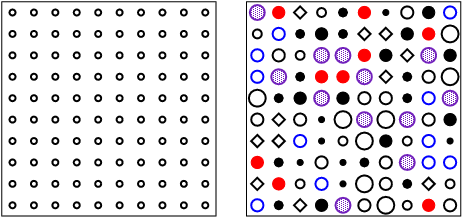
Figure 1: Left: A regular two-dimensional lattice is a periodic arrangement of identical atoms in a rectangular lattice. Right: A disordered lattice whose sites are randomly occupied by different atoms. The closest distance between two neighboring atoms is $a$.

In disordered lattice $W\neq 0$, electron propagation depends on the strength of the disorder. Intuitively, one expects a very weak disorder not to affect the diffusion considerably, but a sufficiently strong disorder should stop the diffusion. Then there should be a critical value $W_{c}$: diffusion continues forever when $W<W_{c}$ but ceases when $W>W_{c}$. In the original paper 1 Anderson derived the equation for the critical disorder as

$${\frac{W_{c}}{V}}=2eK\ln(eK).$$ (3)

According to Eq. (3), the critical disorder depends only on the lattice connectivity $K$ (the number of nearest neighbor sites). Nowadays, we know wegner ; AALR that the dimension $d$ of the lattice is a more important parameter. In the absence of a magnetic field and of electron spin, all states are localized in disordered systems with dimension $d\leq d_{c}=2$. Therefore, the critical disorder $W_{c}=0$ for $d=2$ and is non-zero in systems with higher dimensionality $d>2$.

III Diffusion

Now we demonstrate the Anderson’s ideas in numerical simulation. We examine how the electron diffuses in the disordered lattice, defined by Eq. (2). The size of the system is $L\times L$, where $L=2048a$ for weakly disordered samples and $L=1024a$ for systems with a stronger disorder ($W/V>4$).

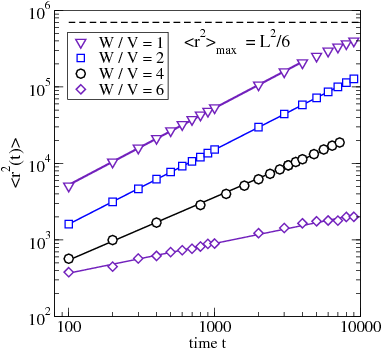
Figure 2: (Color online) The quadratic displacement $\langle r^{2}(t)\rangle$ (in units $a^{2}$) as a function of time $t$. Time is measured in $\hbar/V$. The size of the system is $L\times L$ where $L=2048a$ ($L=1024a$ for $W/V=6$). Note the logarithmic scale of both axes. In weak disorders, we expect the electron to diffuse, so that $\langle r^{2}(t)\rangle=2Dt$, in accordance with Eq. (5). Numerically, we find that $\langle r^{2}\rangle=2Dt^{\alpha}$ with $\alpha=1.004$ for disorder $W/V=1$ and $\alpha=0.98$ for $W/V=2$. The corresponding diffusive constants are $D=25.7$ and $9.1$ (in units $a^{2}V/\hbar$). Only the data for time $t<4000\hbar/V$ were used for $W/V=1$, since in longer time the electron could reach the edge of the sample. The dashed line represents the limit $\langle r^{2}\rangle_{\rm max}=L^{2}/6$, given by Eq. (7). For stronger disorders, the time evolution of the wave function is not diffusive. We find the exponent $\alpha\approx 0.82$ ($W/V=4$) and $\alpha\approx 0.39$ ($W/V=6$).

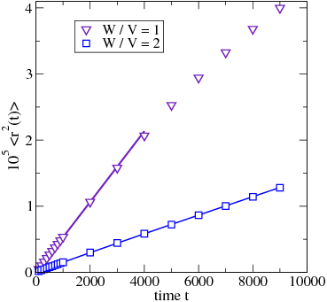
Figure 3: (Color online) The same data as in Fig. 2, but on a linear scale. Only the data for small disorder is shown. Note that for $W/V=1$, $\langle r^{2}(t)\rangle$ is linear only when $t<4000\hbar/V$. This is because the electron already reaches the edge of the sample.

First, we need to define the initial wave function $\Psi(\vec{r},t=0)$. A more suitable candidate than the $\delta$-function (1) is any eigenfunction of the Hamiltonian defined on small sub lattice (typically the size of $24a\times 24a$) located in the center of the sample.ohtsuki Usually we chose the eigenfunction which corresponds to the eigenenergy closest to $E=0$ (the middle of the conductance band).

To see how the initial wave function develops in time $t>0$, we solve the Schrödinger equation (2) numerically and find the time evolution of the wave function $\Psi(\vec{r},t)$. The numerical program is based on the alternating-direction implicit method NRCPS ; elipt used for the solution of elliptic partial differential equations. The algorithm is described in Appendix A.

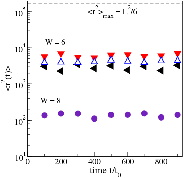
Figure 4: (Color online) Quadratic displacement $\langle r^{2}(t)\rangle$ as a function of time $t/t_{0}$, $t_{0}=1000\hbar/V$ for three systems of the size $L=1024a$ and disorder $W/V=6$ (triangles). Although $\langle r^{2}\rangle$ does not increase when time increases, it fluctuates as a function of time. The limiting value, $R^{2}$ (Eq. 8) depends on the actual realization of the random disorder $\varepsilon(\vec{r})$ in the given sample. the dashed line shows $\langle r^{2}\rangle_{\rm max}=L^{2}/6=174762~{}a^{2}$ which is $50\times$ larger than actual values of $\langle r^{2}\rangle$. For comparison, we also show the quadratic displacement for a system with stronger disorder, $W/V=8$, which is typically $130a^{2}$.

The ability of an electron to diffuse through the sample is measured by a quadratic displacement, defined as

$$\langle r^{2}(t)\rangle=\int d\vec{r}r^{2}|\Psi(\vec{r},t)|^{2}.$$ (4)

Figures 2 and 3 show that in weak disorders, $W/V=1$ and 2, $\langle r^{2}(t)\rangle$ is a linear function of time $t$,

$$\langle r^{2}(t)\rangle=2Dt.$$ (5)

The parameter $D$ is a diffusive constant which enters the Einstein formula for electric conductivity $\sigma$,

$$\sigma=e^{2}D\rho.$$ (6)

Here $e$ is the electron charge and $\rho$ is the density of states.2

Since we analyze only a lattice of a finite size, we have to take into account that the $t$-dependence of the electron wave function might be affected by the finiteness of our sample. In this case, we not only observe the diffusion, but also the reflection of the electron from the edges. Quantitatively, diffusion (5) is observable only when

$$\langle r^{2}(t)\langle\ll\langle r^{2}\rangle_{\rm max}=\frac{1}{L^{2}}\int_{-L/2}^{L/2}\int_{-L/2}^{L/2}\left(x^{2}+y^{2}\right)~{}dxdy=\frac{L^{2}}{6},$$ (7)

where $\langle r^{2}\rangle_{\rm max}$ corresponds to the homogeneously distributed wave function, $|\Psi(\vec{r})|^{2}={\rm const}=1/L^{2}$.

It might seem that the diffusion of electrons shown in Figs. 2 and 3 contradicts the localization theoryAALR that predicts all states to be localized in two-dimensional systems. However, this is not the case. The prediction of the localization theory concerns the limit of an infinite system size. Physically, localization occurs only when the size of the sample exceeds the localization length, $L>\xi$. Since $\xi$ is very large in weak disorder ($\xi\sim 10^{6}a$ when $W=1$),KK we observe metallic behavior and diffusion of electrons in Fig. 2. Of course, even in the case of $W/V=1$ we would observe localization if much larger systems are taken into account.2 In general, we can observe the localization if we either increase the size of the system or reduce the localization length. The latter is easier to perform, as it requires us only to increase the disorder strength $W$. We will do it in the next Section.

IV Absence of diffusion - localization

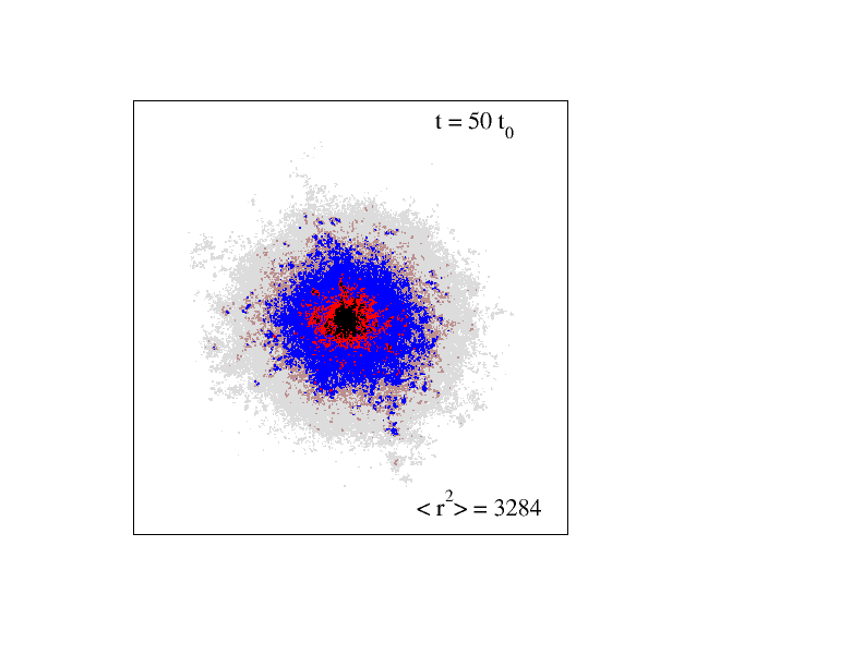
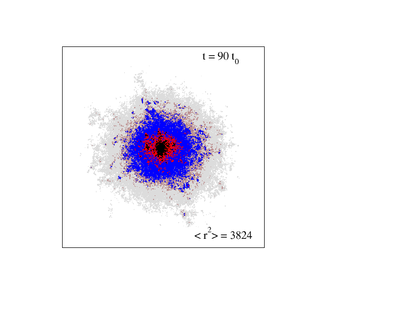
Figure 5: (Color online) Spatial distribution of an electron in sample with disorder $W/V=6$. The size of the lattice is $1024a\times 1024a$. Time is given in units of $t_{0}=1000\hbar/V$. The different colors show sites where $|\Psi(r)|>10^{-4}$ (gray), $>5\times 10^{-4}$ (brown), $10^{-3}$ (blue), $5\times 10^{-3}$ (red), and $>5\times 10^{-3}$ (black). The probability to find an electron on any other site is less than $10^{-8}$.

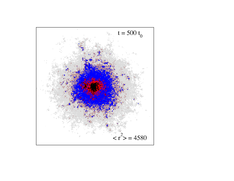
Figure 6: (Color online) The same as in Fig. 5 only the time is $t=500t_{0}$ and $900t_{0}$ ($t_{0}=1000\hbar/V$).

The data in Fig. 2 also confirms that the time evolution of the wave function is not diffusive when the disorder $W$ increases. Linear increase of $\langle r^{2}(t)\rangle$ is observable only for short initial time interval. For any longer time, the spatial extent of the electron increases very slowly and finally ceases (Fig. 4). the electron becomes localized.

To demonstrate the electron localization more explicitly, we repeat the experiment in Section III with a stronger disorder $W/V=6$. Similarly to the previous experiment, the initial wave function is non-zero in the small area $24a\times 24a$ located at the center of the sample. For shorter times, we observe that the spatial extent of the wave function increases. Then, after a while, $\langle r^{2}(t)\rangle$ saturates:

$$\lim_{t\to\infty}\langle r^{2}(t)\rangle=R^{2}\ll\langle r^{2}\rangle_{\rm max}.$$ (8)

Although the spatial distribution of the electron varies in time, $\langle r^{2}(t)\rangle$ does not longer increase even if the time $t$ increases ten and more times.

Figures 5 and 6 show the spatial distribution of the wave function, $|\Psi(\vec{r},t)|$. they represent the lattice sites with $|\Psi(\vec{r})|>10^{-4}$. This means that the probability to find the electron in any other lattice site is less than $10^{-8}$.

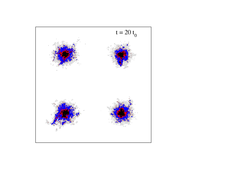
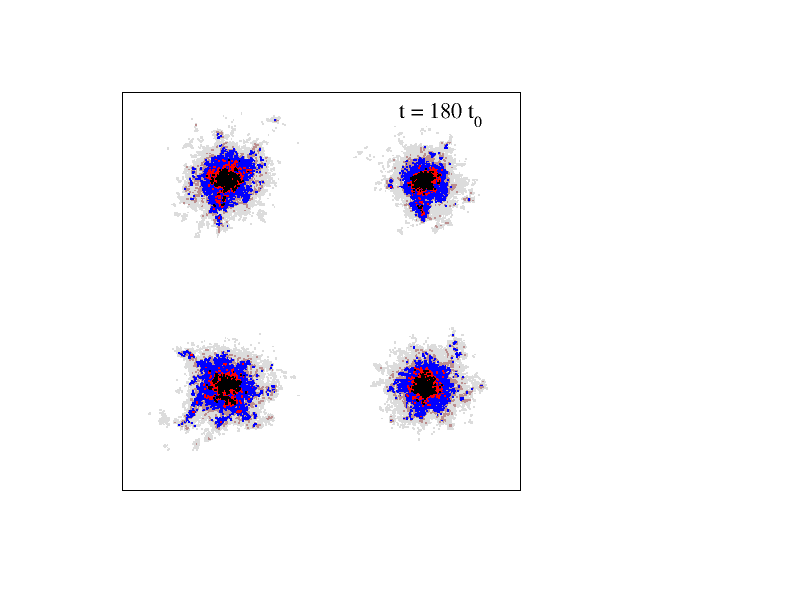
Figure 7: (Color online) The time development of four electrons located in time $t=0$ in four different areas of the same lattice. The electrons do not leave the initial areas. The size of the sample is $L=1024a$. Disorder $W/V=8$. Again, time is measured in units of $t_{0}=1000\hbar/V$.

Note that there is no potential well in the center of the sample where the electron is localized. The only reason for the electron being localized in the lattice center is the initial wave function, $\Psi(\vec{r},t=0)$, which was non-zero only in the center of the lattice. Applying the initial wave function localized in any other area of the sample, we would achieve electron localization in that area. This is demonstrated in Fig. 7 showing the time development of the wave functions of four electrons in the same lattice. The initial position of the electrons is centered around four points

$$x_{\pm}=L/2\pm L/4,~{}~{}~{}~{}y_{\pm}=L/2\pm L/4.$$ (9)

We see that in time $t>0$ each electron is localized around its initial position. This proves that localization is indeed the result of interference of wave functions. The electron is not trapped in any potential well. The localized state is not a bound state.

Figure 7 also shows that the localized states are very sensitive to the realization of the random potential. The spatial distribution of each electron reflects the local distribution of random energies $\varepsilon(\vec{r})$. This is shown quantitatively in Fig. 4 where we plot $\langle r^{2}(t)\rangle$ as a function of time for three different realizations of the random disorder. We see that although all three samples have the same macroscopic parameter $W/V=6$, the limiting value $R^{2}=\lim_{t\to\infty}\langle r^{2}(t)\rangle$ is not universal but depends on the actual distribution of random energies in the given sample. Moreover, $\langle r^{2}(t)\rangle$ fluctuates as a function of time $t$.

V Transmission through disordered sample: How an electron propagates through disordered system?

Consider now another experiment, frequently used in the mesoscopic physics: We take a disordered sample, the same as used in previous Sections, to examine what is the probability that an electron propagates from one side of the sample to the opposite side. Both in experiments and in numerical simulations the sample is connected to two semi-infinite, disorder-free leads which guide the electron propagation towards and out of the sample (Fig. 8). An incoming electron either propagates through the sample or is reflected back. The probability of transmission, $T$, determines the conductance, SE ; landauer

$$g=\displaystyle{\frac{e^{2}}{h}}~{}T.$$ (10)

Eq. (10) is commonly referred to as the Landauer formula. It was originally derived for a one-dimensional system but can also be used for the analysis of two- and more-dimensional samples. Since the width of the leads is non-zero the transmission $T$ can be larger than 1. comment The transmission is calculated by the transfer matrix method described in Refs. Ando-91 ; PMcKR ; 2 .

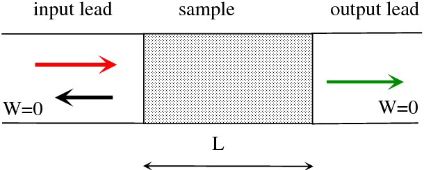
Figure 8: Schematic description of the scattering experiment for measurement of the transmission. The sample is connected to two semi-infinite leads represented by regular lattice with zero disorder. Inside the sample, the disorder is non-zero. If electron comes from the left, it either propagates through the sample and contributes to the transmission, or is reflected back to the left lead.

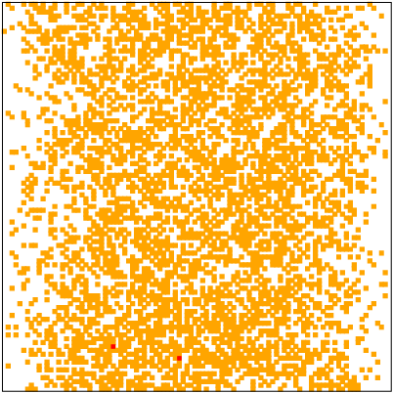
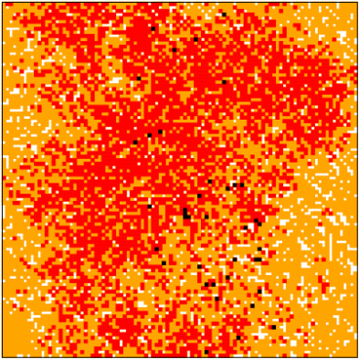
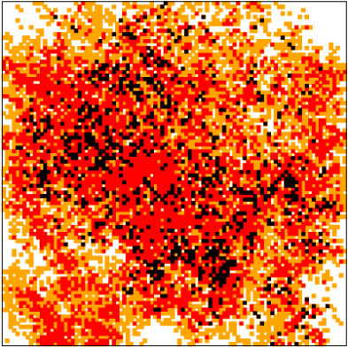
Figure 9: (Color online) Sensitivity of the transmission trough the disordered system to the change of the sign of a single random energy $\vec{r}_{0}$. A change of the sign of the random energy on orange, red and black sites causes the change of the conductance by more than 1%, 10% and 100%, respectively. The transmission $T$ is $4.998$, $0.52$ and 0.00084 for the disorder $W/V=2$, 4 and 6 (from top to bottom). The size of the system is $100a\times 100a$, and the electron propagates from the left side of the sample to the right side.

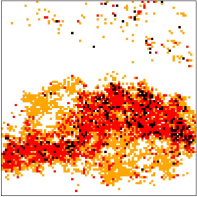
Figure 10: (Color online) The same as in Fig. 9 but disorder $W/V=10$. The transmission $T=9\times 10^{-15}$.

Contrary to the diffusion problem, discussed in Sects. III,IV, in the present experiment we do not analyze the time development of the electron wave function. Instead, we chose the energy $E$ of the electron ($E=0$, that is the center of the energy band), and calculate the time independent current transmission $T$ from the left side of the sample to the right side.

To show how electrons are distributed within the sample, we apply Pichard’s idea. PNato Let us change the sign of a single random energy $\epsilon(\vec{r}_{0})$ at a site $\vec{r}_{0}$: $\epsilon(\vec{r}_{0})\to-\epsilon(\vec{r}_{0})$ and calculate how this change will influence the total transmission $T$ of an electron through the sample. We expect that $T$ is sensitive to the change of $\epsilon(\vec{r}_{0})$ only if the electron occupies the site $\vec{r}_{0}$, i.e. when $|\Psi(\vec{r}_{0})|$ is large. Contrary, if $|\Psi(\vec{r}_{0})|$ is negligible, then the change of $\epsilon(\vec{r}_{0})$ cannot affect the transmission $T$.

Thus, by the comparison of the transmissions through two systems differing only in the sign of the random energy $\varepsilon(\vec{r}_{0})$, we can estimate whether the electron, propagating through the sample, travels through the site $\vec{r}_{0}$ or not. In repeating this analysis for all lattice sites, we can visualize the path of the electron through the sample. For numerical reasons, we restricted the sample size to $100a\times 100a$.

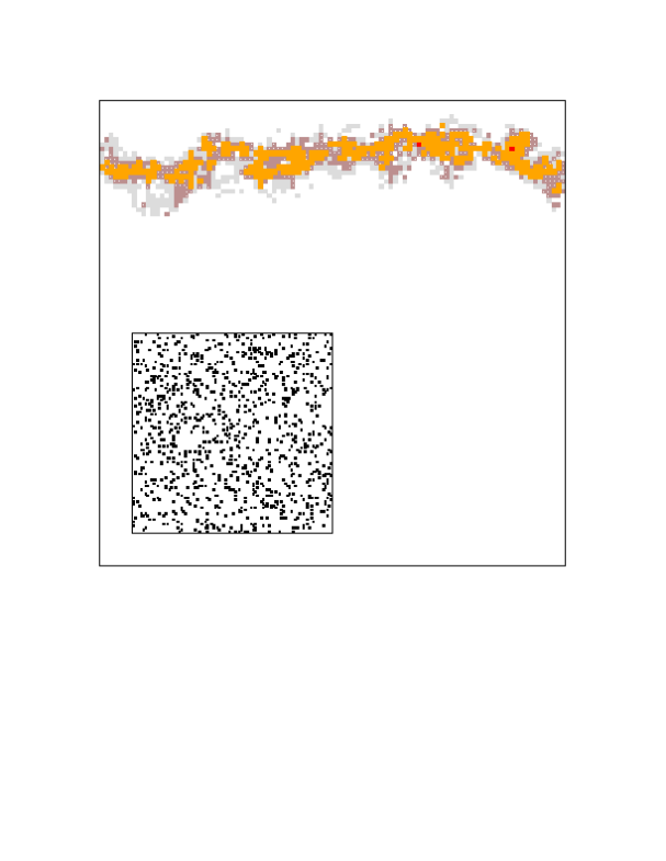
Figure 11: (Color online) The same as in Fig. 9 but for disorder $W/V=20$. The transmission is really small, $\ln T=-96$. The change of the sign of the random energy on gray, brown, orange and red sites causes a change of the logarithm of the transmission by more than 0.01%, 0.1%, 1% and 10% respectively. Although it seems that the path through the sample is determined by a valley in the potential landscape, this is not the case. The inset shows sites of the sample where the random energy $|\epsilon|<1$.

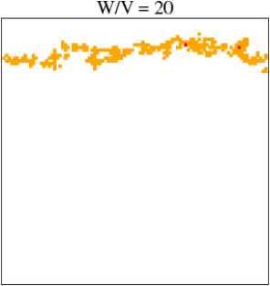
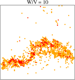
Figure 12: (Color online) The electron path through two strongly disordered samples: both samples have the same realization of random energies. They differ only in the amplitude of fluctuations. Shown are the lattice sites where the change of the sign of random energy causes the change of the logarithm of the transmission by 1% (orange) and 10% (red). We see that the electron prefers completely different trajectories through these samples.

Our results are summarized in Fig. 9. In weak disorders, $W/V=2$, we see that the changing of only one random energy has an almost negligible influence on the transmission. Typically, $T$ changes only by 1% (or even less) when the sign of $\varepsilon(\vec{r})$ changes. Also, all lattice sites are more or less equivalent. We conclude that in the course of the transmission the electron is “everywhere”: it propagates through the entire sample as a quantum wave. This observation is the key idea of the Dorokhov-Mello-Pereyra-Kumar theory of the electron transport in weakly disordered systems DMPK and of the random matrix theory of diffusive transport. PNato

The homogeneity of the electron distribution gets lost when the disorder increases.muttalib ; MMW The change of the random energy sign on some sites influences the transmission more than the same change on other sites. Some areas of the sample seem not to be visited at all. We can see the formation of the electron “path” through the sample.prior This path is clearly visible for very strong disorder shown in Figs. 10, 11 and 12.

However, we want to stress that even in case of strong disorders we cannot speak about the path in its classical sense. Even if the electron path is well visible, there are still other sites, often located on the opposite side of the sample, that influence the transmission as strongly as the sites on the main trajectory (Fig. 10). This indicates that the electron still feels the entire sample and its propagation is highly sensitive to any change of the realization of the random potential.

the resulting trajectory cannot be identified with any valley or equipotential line in the random potential landscape. To demonstrate this, we show in Fig. 11 the trajectory of an electron through an extremely strongly disordered system ($W/V=20$ - in this case, we consider the change of the logarithm of the conductance). Although the trajectory of an electron seems to be well defined, there is no continuous potential valley which might support the propagation. The inset of Thus, the choice of the transmission path is the result of quantum interference: an electron arising from the left inspects the entire sample and finds the most convenient spatial “channel” for its propagation. We cannot speak about a trajectory in the sense of classical particles.

To support our last claim, let us consider two samples, with the same realization of random energies $\varepsilon(\vec{r})$, but different amplitudes of random energies: $W/V=10$ for the sample I and $W/V=20$ for the sample II:

$$\varepsilon(\vec{r})^{II}=2\varepsilon(\vec{r})^{I}$$ (11)

for each site $\vec{r}$. With the help of the above-mentioned method, we find the trajectories of electrons through these two samples. For the propagation of classical particle both trajectories (for the sample I and sample II) should coincide. However, an electron is not a classical particle. As shown in Fig. 12, the ways how an electron propagates through the two samples, I and II, are completely different. An increase of fluctuations of the random potential causes the electron to choose a completely different route.

VI Conclusion

We discussed two features of localization of quantum particle in a disordered sample. Firstly, we demonstrated numerically that the diffusion of the quantum particle through randomly fluctuating potential ceases after certain time. The particle becomes spatially localized. The physical origin of localization is different from the bounding of a particle in a potential well. Localization is caused by a multiple scattering of the wave function on randomly distributed impurities (fluctuations of the random potential). It is not due to the trapping of the particle in the potential well.

In the second part of the paper, we examined the propagation of a quantum particle through a disordered sample and discussed how this propagation depends on the disorder. Again, we confirmed indirectly the wave character of the propagation. This drove us to the conclusion that the electron localization is a purely quantum effect without any analogy in classical mechanics.

In both numerical experiments, the key condition for the localization to happen is the quantum coherence of the wave function. This is generally not fulfilled in experiment, where the incoherent scattering - for instance the scattering of electrons with phonons - plays the crucial role. As any incoherent scattering destroys quantum coherence, the observing of electron localization experimentally requires the mean free path of incoherent scattering to be larger or at least comparable to size of the sample. This happens at a very low temperature. Of course, localization does affect the transport of electrons also at higher temperatures. These effects are, however, above the scope of present discussion.

With localization being a wave phenomenon, we can expect the similarity of quantum propagation with classical wave phenomena. dragoman That enables us to observe localization in many other instances. In particular, we can expect that classical waves - electromagnetic or acoustic - will also be localized in a disordered medium. S The localization of microwave electromagnetic waves was experimentally observed GG . Another very interesting experimentqq proves the weak localization of seismic waves.

Appendix A Numerical solution of the Schrödinger equation

To integrate the Schrödinger equation (2) numerically, we first have to discretize the time derivative:

$${\frac{\partial\Psi(\vec{r},t)}{\partial t}}=\frac{1}{\delta t}\left[\Psi(\vec{r},t+\delta t)-\Psi(\vec{r},t)\right],$$ (12)

where $\delta t$ is the time iteration step. In order to define the iteration procedure for the calculation of the wave function in $\Psi(\vec{r},t+\delta)$ in terms of $\Psi(\vec{r},t)$, we also have to determine the time in which the wave function on the right-hand side of Eq. (2) is calculated. The explicit method takes the entire r.h.s. of Eq. (2) in time $t$. The resulting iteration scheme is simple, the time step $\delta t$, however, has to be very small to avoid numerical instabilities.NRCPS Other, more sophisticated, explicit methods based on the Suzuki-Trotter formula are described in Ref.ohtsuki In this paper, we use the alternating-direction implicit iteration schema. NRCPS ; elipt This method presses the numerical integration of Schrödinger equation (2) in two steps. Firstly, we write the Schrödinger equation (2) in its discrete form ($\vec{r}=(x,y)$)

$$\begin{array}[]{ll}\Psi(x,y,t+\delta t)&=\Psi(x,y)+\displaystyle{\frac{V}{i\hbar}}\delta t\Big{[}\frac{W}{V}\varepsilon(x,y)\Psi(x,y,t)\\ &\\ &+\Psi(x+a,y,t+\delta t)+\Psi(x-a,y,t+\delta t)\\ &\\ &+\Psi(x,y+a,t)+\Psi(x,y-a,t)\Big{]}\end{array}$$ (13)

Note that the wave function along the $x$ direction is in time $t+\delta t$, while the wave function in $y$ direction is in time $t$. The second step is to put $t\to t+\delta t$ and re-write the iteration equation in the form

$$\begin{array}[]{ll}\Psi(x,y,t+\delta t)&=\Psi(x,y)+\displaystyle{\frac{V}{i\hbar}}\delta t\Big{[}\frac{W}{V}\varepsilon(x,y)\Psi(x,y,t)\\ &\\ &+\Psi(x+a,y,t)+\Psi(x-a,y,t)\\ &\\ &+\Psi(x,y+a,t+\delta t)+\Psi(x,y-a,t+\delta t)\Big{]}.\end{array}$$ (14)

Now the wave function along the $y$ direction is given in time $t+\delta t$ and the wave function along $x$ direction is in time $t$.

The advantage, that this algorithm presents is its numerical stability, even for rather large values of $\delta t$. The price for the numerical stability is that we have to solve $N$ ($N=L/a$) systems of $N$ linear equations in each iteration step. Fortunately, iteration schema (13,14) only requires solution of the three-diagonal system of linear equations, what is easy to calculate.

Other modifications of the above algorithm are possible since we are free to substitute the wave function $\Psi(x,y,t)$ on the r.h.s of Eqs. (13,14) by $\Psi(x,y,t+\delta t)$, or, eventually, by $[\Psi(x,y,t)+\Psi(x,y,t+\delta t)]/2$.

To measure the accuracy of the numerical solution, we also calculate in each time $t$ the norm of the wave function,

$${\cal N}=\int d\vec{r}|\Psi(\vec{r},t)|^{2}.$$ (15)

We obtained that for $\delta t=0.1\hbar/V$ the norm ${\cal N}$ is always very close to 1:

$$|{\cal N}-1|<2\times 10^{-3}.$$ (16)

This work was supported by project APVV n. 51-003505 and project VEGA 2/6069/26.

References

- (1) P. W. Anderson, Phys. Rev. 109, 1492 (1958).
- (2) B. Kramer and A. MacKinnon, Rep. Prog. Phys 56, 1469 (1993).
- (3) M. Janßen, Int. J. Mod. Phys. B 8, 943 (1994).
- (4) J. M. Ziman, J. Phys. C 1, 1532 (1968); ibid 2, 1232, (1969); 2, 1704 (1969).
- (5) P. W. Anderson, D. J. Thouless, E. Abrahams and D. S. Fisher, Phys. Rev. B 22, 3519 (1980).
- (6) P. Markoš and C. M. Soukoulis, Wave Propagation: From Electrons to Photonic Crystals and Left-handed Materials, Princeton Univ. Press (2008).
- (7) P. Markoš, acta physica slovaca 56, 561 (2006), available at http://www.kf.elf.stuba.sk/markos/acta.pdf; also cond-mat/069580.
- (8) P. A. Lee, A. D. Stone, Phys. Rev. Lett. 55, 1622 (1985); Phys. Rev. B 35, 1039 (1987).
- (9) O. N. Dorokhov, JETP Lett. 36, 318 (1982); P. A. Mello, P. Pereyra and N. Kumar, Ann. Phys. (NY) 181, 290 (1988).
- (10) J.-L. Pichard: in: B. Kramer (ed.) Quantum Coherence in Mesoscopic Systems, NATO ASI 254, Plenum Press NY and London (1991), p. 369.
- (11) C. W. J. Beenakker, Rev. Mod. Phys. 69,731 (1997).
- (12) J.-L. Pichard, G. Sarma, J. Phys. C, 14 L127 (1981); ibid, L167
- (13) A. MacKinnon, B. Kramer Phys. Rev. Lett., 47, 1546 (1981).
- (14) A. MacKinnon and B. Kramer, Z. Phys. B 53, 1 (1983).
- (15) E. N. Economou, Green’s Functions in Quantum Physics, 2nd ed. Springer, Berlin (1979).
- (16) F. Wegner, Z. Phys. B 25, 327 (1976); ibid 35, 207 (1979).
- (17) E. Abrahams, P. W. Anderson, D. C. Licciardello and T. V. Ramakrishnan, Phys. Rev. Lett. 42, 673 (1979).
- (18) T. Kawarabayashi and T. Ohtsuki, Phys. Rev. B 51, 10897 (1995); Phys. Rev. B 53, 6975 (1996).
- (19) W. H. Press, S. A. Teukolsky, W. T. Vetterling and B. P. Flannery, Numerical Recipes in Fortran 77, The Art of Scientific Computing, 2nd ed. Cambridge Univ. Press (1992).
- (20) D. W. Peaceman, H. H. Rachford, J. Soc. Indust. Appl. Math. 3, 28 (1955).
- (21) E. N. Economou and C. M. Soukoulis, Phys. Rev. Lett. 46, 618 (1981); ibid 47 973 (1981).
- (22) R. Landauer, IBM J. Res. Dev. 1, 223 (1957); Phil. Mag. 21, 683 (1970).
- (23) For non-zero width of leads, the wave function in leads is a superposition of different modes. Each mode is characterized by its transverse momentum, . Since the electron is a quantum particle, is quantized. For each transversely wave vector, we have a longitudinal component given by the dispersion relation . Note that some values of might be imaginary. these modes are called evanescent. They do not transfer the current in leads, contrary to propagating modes with real . If we have propagating modes, then , where is the probability that an electron coming from the left with a wave vector appears on the opposite side of the sample with the wave vector . Since , the maximum of is .
- (24) T. Ando, Phys. Rev. B 44, 8017 (1991).
- (25) J. B. Pendry, A. MacKinnon and P. J. Roberts, Proc. R. Soc. London A 437, 67 (1992).
- (26) K. A. Muttalib and J. R. Klauder, Phys. Rev. Lett. 82, 4272 (1999); K. A. Muttalib and V. A. Gopar, Phys. Rev. B 66, 115318 (2002).
- (27) K. A. Muttalib, P. Markoš and P. Wölfle, Phys. Rev. B 72, 125317 (2005); cond-mat/0501101
- (28) A. M. Somoza, M. Ortuno and J. Prior, Phys. Rev. Lett. 99, 116602 (2007).
- (29) D. Dragoman, M. Dragoman, Quantum - Classical Analogies. Springer (2004)
- (30) C. M. Soukoulis, E. N. Economou, G. S. Grest and M. H. Cohen, Phys. Rev. Lett. 62, 575 (1989).
- (31) N. Garcia and A. Z. Genack, Phys. Rev. Lett. 66, 1850 (1991); A. Z. Genack and N. Garcia, Phys. Rev. Lett. 66, 2064 (1991).
- (32) E. Larose, L. Margerin, B. A. van Tiggelen and M. Campillo, Phys. Rev. Lett. 93, 048501 (2004).