Entanglement in a Raman-driven cascaded system

Abstract

The dynamics of a cascaded system that consists of two atom-cavity subsystems is studied by using the quantum trajectory method. Considering the two atom-cavity subsystems driven by a Raman interaction, analytical solutions are obtained. Subsequently, the entanglement evolution between the two atoms is studied, and it is shown that the entanglement can be stored by switching off the Raman coupling. By monitoring the radiation field, the entanglement between the two atoms can be enhanced.

I Introduction

The concept of entanglement has been of great interest since the early days of quantum mechanics Schroedinger , and it has become of central importance in a variety of discussions on the fundamental aspects of the theory Einstein ; Bell . Nowadays entanglement is receiving new attention in the context of the rapidly developing fields of quantum information, quantum computation and quantum technology; for reviews, see Nielsen ; HarocheRaimond ; Kok:135 ; Chen . Entanglement is considered to be the characteristic feature that allows quantum information to overcome some of the limitations imposed by classical information. Cold trapped atoms interacting with quantized light fields are promising candidates for the realization of quantum computing and quantum communication protocols Monroe:238 ; Mabuchi:1372 . The combination of long-lived atomic states and light fields can be used in quantum networking for the distribution and processing of quantum information Cirac:3221 ; Knill:46 . In the context of entanglement preparation between atoms at separate nodes, a variety of schemes have been proposed, for example, by measuring the superpositions of light fields released from separate atomic samples, or by measuring a probe light field that has interacted in a prescribed way with different samples. Due to the indistinguishability in the measurement, and conditioned on the results of the measurements, the atomic system is projected into an entangled state Bose:5158 ; Duan:253601 ; Duan:5643 ; Duan:413 . An unconditional preparation of entanglement has also been analyzed in the case of a cascaded system. This unconditional preparation has been discussed for two distantly separated atoms Clark:177901 ; Gu:043813 , as well as for separate atomic ensembles Parkins:053602 . Moreover, the recent achievements in cavity QED and in tapped ion techniques have rendered it possible to experimentally generate pairs of entangled atoms Hagley:1 , to create entangled states of several atoms Leibfried:639 , and even long-lived entanglement of two macroscopic ensembles of atoms Julsgaard:400 .

In the spirit of these previous achievements, in the present contribution we will consider the quantum trajectory approach for a cascaded open quantum system Carmichael:2273 . We study the dynamics of a system that consists of two atom-cavity sub-systems $A$ and $B$. The quantum source $A$ emits a photon and the second quantum subsystem $B$ reacts on the emitted photon. We will first consider an unconditional preparation of the entanglement between the two atoms. Second, the effects of a null-measurement conditional preparation is analyzed with respect to a photodetector of a given efficiency monitoring the field radiated by the cascaded system.

As is clearly discussed in Refs. Clark:177901 ; Gu:043813 ; Parkins:053602 , the advantage in using a cascaded system is that the dynamical evolution of the open quantum system itself creates the entanglement. It is an unconditional preparation, and it is not related to a “click” or “no click” at a detector, where the measurement projects the atomic system onto the desired entangled state. In this sense, we can say that it is a dynamical generation of entanglement, and not a conditional one. One could also use a detector of given efficiency to monitor the radiated field, to prepare the system conditioned upon “no click” at the detector. This allows us to realize a quantum state preparation conditioned upon the limited knowledge of the observer’s imperfect detector. In this way one can combine the advantages of using a cascaded system, with its intrinsic dynamical generation of entanglement, and a conditional preparation with a detector of non-unit efficiency. In the case under study the entanglement between the two atoms can only increase due to this conditional preparation, even for imperfect detection. In the limiting case of a detector of zero efficiency, we return to the case of unconditional preparation, where only dynamically generated entanglemet is present. In the system under study we consider a Raman configuration for driving the atom-cavity interaction. By switching off the lasers beams, the Raman interaction vanishes, so that the entanglement generated between the atoms remains unchanged and can be stored.

The paper is organized as follows. In Sec. II the master equation describing the dynamics of the cascaded system is introduced, and the problem is solved analytically by using the quantum trajectory method. In Sec. III the unconditional preparation and storage of the entanglement between the two atoms is analyzed. The conditional preparation of the entanglement between the two atoms is discussed in Sec. IV. Finally, some concluding remarks are given in Sec. V.

II Cascaded system dynamics

In this section we analyze the dynamics of the system under study. The cascaded open quantum system consists of two atom-cavity subsystems $A$ and $B$, where the source subsystem $A$ is cascaded with the target subsystem $B$, as sketched in Fig. 1. The cavities have three perfectly reflecting mirrors and one mirror with transmission coefficient $T\ll 1$. In the two subsystems $A$ and $B$, denoted by $k=a,b$, respectively, we consider a three-level atom coupled to a cavity mode of frequency $\omega_{k}$ via a Raman interaction, as indicated in Fig. 2. This configuration is obtained by irradiating the atom with a laser beam of frequency $\omega_{k}^{\prime}$ such that $\omega_{k}-\omega_{k}^{\prime}=\omega_{10}^{k}$, where $\omega_{10}^{k}$ is the transition frequency between the two atomic energy eigenstates $|1_{k}\rangle$ and $|0_{k}\rangle$. The laser beam is detuned from the electric dipole transition $|1_{k}\rangle\leftrightarrow|2_{k}\rangle$ by $\Delta_{k}$, chosen to enhance the Raman-coupling strength, but also to avoid electronic excitations. The Rabi frequency of the laser is denoted by $\Omega_{k}$ and $g_{k}$ is the strength of coupling between the cavity mode and the $|0_{k}\rangle\leftrightarrow|2_{k}\rangle$ transition. The cavity mode is damped by losses through the partially transmitting cavity mirror. In addition to the wanted outcoupling of the field, the atom can spontaneously emit a photon out the side of the cavity, or a photon can be absorbed or scattered by the cavity mirrors.

To describe the dynamics of the system we will use a master equation formalism, and solve it by using the quantum trajectory method Dalibard:580 ; Dum:4382 ; Carmichael1 . For sufficiently large detuning, $g_{k}/\Delta_{k}$ and $\Omega_{k}/\Delta_{k}\ll 1$, the excited state $|2_{k}\rangle$ will not become significantly populated and can be adiabatically eliminated. This leads, treating the dissipation due to the cavity losses in a standard way Haake ; Louisell ; Davies , to the following master equation for the reduced density operator $\hat{\rho}(t)$ of the system:

$$\frac{d\hat{\rho}(t)}{dt}\!\!\! = \!\!\!\frac{1}{i\hbar}\!\left[\hat{H},\hat{\rho}(t)\right]\!+\!\sum_{i=1}^{7}\left[\hat{J}_{i}\hat{\rho}(t)\hat{J}_{i}^{\dagger}-\frac{1}{2}\hat{J}_{i}^{\dagger}\hat{J}_{i}\hat{\rho}(t)\right.$$ (1)

$$- \left.\frac{1}{2}\hat{\rho}(t)\hat{J}_{i}^{\dagger}\hat{J}_{i}\right].$$

The Hamiltonian is given by

$$\hat{H}=\hat{H}_{A}+\hat{H}_{B}+i\hbar\frac{\sqrt{\kappa_{a}\kappa_{b}}}{2}\left(e^{-i\phi}\hat{b}\hat{a}^{\dagger}-e^{i\phi}\hat{b}^{\dagger}\hat{a}\right)\,,$$ (2)

where $\hat{H}_{A}$ and $\hat{H}_{B}$ describe the atom-cavity interaction in the two subsystems $A$ and $B$, respectively. In the rotating-wave approximation they are given by Difidio:105

$$\hat{H}_{A}=\hbar\bar{g}_{a}\left(\hat{a}\hat{A}_{10}+\hat{a}^{\dagger}\hat{A}_{01}\right)+\hbar\Delta_{a}^{\prime}{\hat{A}}_{11}+\hbar\bar{\Delta}_{a}\hat{a}^{\dagger}\hat{a}{\hat{A}}_{00}\,,$$ (3)

and

$$\hat{H}_{B}=\hbar\bar{g}_{b}\left(\hat{b}\hat{B}_{10}+\hat{b}^{\dagger}\hat{B}_{01}\right)+\hbar\Delta_{b}^{\prime}{\hat{B}}_{11}+\hbar\bar{\Delta}_{b}\hat{b}^{\dagger}\hat{b}{\hat{B}}_{00}\,.$$ (4)

The third term in Eq. (2) describes the coupling between the two cavities Carmichael:2273 ; Gardiner:2269 . In these expressions, $\hat{a}$ and $\hat{a}^{\dagger}$ are annihilation and creation operators for the cavity field $A$, and similarly $\hat{b}$ and $\hat{b}^{\dagger}$ for the cavity field $B$. We have also defined $\hat{A}_{ij}=|i_{a}\rangle\langle j_{a}|$ ($i,j=0,1$), and $\hat{B}_{ij}=|i_{b}\rangle\langle j_{b}|$ ($i,j=0,1$). In addition, $\bar{g}_{k}\!=\!-g_{k}\Omega_{k}/\Delta_{k}$ is the effective atom-cavity coupling constant and $\Delta_{k}^{\prime}\!=\!-\Omega_{k}^{2}/\Delta_{k}$, $\bar{\Delta}_{k}\!=\!-g_{k}^{2}/\Delta_{k}$ are the two Stark shift terms. Moreover, $\kappa_{a}$, $\kappa_{b}$ are the cavity bandwidths and the phase $\phi$ is related to the phase change upon reflection from the source output mirror, and/or to the retardation of the source due to the spatial separation between the source and the target, cf. Carmichael2 .

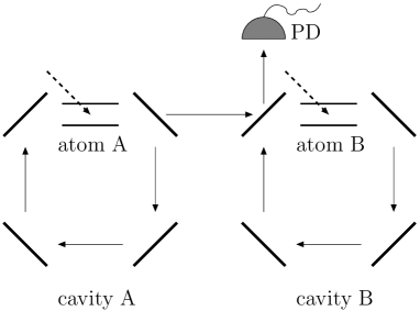
Figure 1: The cascaded open system consisting of two Raman-driven atom-cavity subsystems $A$ and $B$. The dashed arrows indicate the laser fields needed for the Raman coupling. A photodetector PD can be used to monitor the radiation field.

The jump operators $\hat{J}_{i}$ in Eq. (1) are defined by

$$\hat{J}_{1}=\sqrt{\kappa_{a}}\hat{a}+\sqrt{\kappa_{b}}e^{-i\phi}\hat{b}\,,$$ (5)

which describes a photon emission by the cavities;

$$\hat{J}_{2}=\sqrt{\kappa_{a}^{\prime}}\hat{a}\,,~{}~{}~{}~{}~{}~{}~{}\hat{J}_{3}=\sqrt{\kappa_{b}^{\prime}}\hat{b}\,,$$ (6)

are associated with a photon absorption or scattering by the cavity mirrors;

$$\hat{J}_{4} = \sqrt{\Gamma_{a}}\!\left(\!\Omega_{a}\hat{A}_{01}\!+\!g_{a}\hat{a}\hat{A}_{00}\!\right),$$

$$\hat{J}_{5} = \sqrt{\Gamma_{a}^{\prime}}\!\left(\!\Omega_{a}\hat{A}_{11}\!+\!g_{a}\hat{a}\hat{A}_{10}\!\right)\!,$$ (7)

and

$$\hat{J}_{6} = \sqrt{\Gamma_{b}}\!\left(\!\Omega_{b}\hat{B}_{01}\!+\!g_{b}\hat{b}\hat{B}_{00}\!\right),$$

$$\hat{J}_{7} = \sqrt{\Gamma_{b}^{\prime}}\!\left(\!\Omega_{b}\hat{B}_{11}\!+\!g_{b}\hat{b}\hat{B}_{10}\!\right)\!,$$ (8)

are related to a photon spontaneously emitted by the atoms. Here $\kappa_{k}^{\prime}$ is the cavities mirrors’ absorption and scattering rate. Moreover, $\Gamma_{k}\!=\!\gamma_{k}/\Delta_{k}^{2}$ and $\Gamma_{k}^{\prime}\!=\!\gamma_{k}^{\prime}/\Delta_{k}^{2}$, where $\gamma_{k}$ and $\gamma_{k}^{\prime}$ are the dipole relaxation rates of the atomic state $|2_{k}\rangle$ to the states $|0_{k}\rangle$ and $|1_{k}\rangle$, respectively. These relaxation rates are considered to be small in comparison with the detuning. Note that the operator $\hat{J}_{1}$ contains the superposition of the two fields radiated by the two cavities, due to the fact that radiated photons cannot be associated with photon emission from either $A$ or $B$ separately Carmichael:2273 .

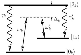
Figure 2: Raman-type excitation scheme for the atom-cavity subsystem $A$ ($k=a$) and $B$ ($k=b$). The cavity mode of frequency $\omega_{k}$ and the laser of frequency $\omega_{k}^{\prime}$ are detuned by $\Delta_{k}$ from the atomic state $|2_{k}\rangle$. The dipole relaxation rates of these states to the states $|0_{k}\rangle$ and $|1_{k}\rangle$ are $\gamma_{k}$ and $\gamma_{k}^{\prime}$, respectively.

In the following we will identify, for notational convenience, the state $|a\rangle$ with the state $|1,0,0,0\rangle$, which denotes the atom $A$ in the state $|1_{a}\rangle$, the cavity $A$ in the vacuum state, the atom $B$ in the state $|0_{b}\rangle$ , and the cavity $B$ in the vacuum state. In the state $|b\rangle\equiv|0,1,0,0\rangle$ the atom $A$ is in the state $|0_{a}\rangle$, and the cavity $A$ is in the one-photon Fock state. Similarly, we define $|c\rangle\equiv|0,0,1,0\rangle$, $|d\rangle\equiv|0,0,0,1\rangle$, and $|e\rangle\equiv|0,0,0,0\rangle$. The state $|a\rangle$ will be considered as the initial state of the system. It follows that the Hilbert space that describes the cascaded system under study is, in our model, spanned by the five state vectors $|a\rangle$, $|b\rangle$, $|c\rangle$, $|d\rangle$, and $|e\rangle$.

To evaluate the time evolution of the system we use a quantum trajectory approach Dalibard:580 ; Dum:4382 ; Carmichael1 . Note that the probability for a jump $\hat{J}_{i}$ to occur in the time interval $[t,t+dt)$ is given by $p_{\rm i}(t)\!=\!\langle\hat{J}_{i}^{\dagger}\hat{J}_{i}\rangle_{t}\,dt$. This implies that the total probability for a jump due to a spontaneous emission in the time interval $[t,t+dt)$ is given, using Eqs. (7), (8), (3), and (4), by

$$\sum_{i=4}^{7}\langle\hat{J}_{i}^{\dagger}\hat{J}_{i}\rangle_{t}dt=-\frac{\gamma_{a}+\gamma_{a}^{\prime}}{\hbar\Delta_{a}}\langle\hat{H}_{A}\rangle_{t}dt-\frac{\gamma_{b}+\gamma_{b}^{\prime}}{\hbar\Delta_{b}}\langle\hat{H}_{B}\rangle_{t}dt.$$ (9)

This relation shows that in a time interval $\sim\Delta/(g\Omega)$ the probability to have a jump due to spontaneous emissions is $\sim(\gamma_{a}\!+\gamma_{a}^{\prime}\!+\gamma_{b}\!+\gamma_{b}^{\prime})/\Delta$, cf. Wineland:2977 . For a large detuning this probability is small. If one is interested to follow the dynamical evolution of the system for several Rabi oscillations, in general the effects due to spontaneous emissions cannot be neglected Difidio:031802 . In the present contribution, the Raman dynamics would be actually used only for a few Rabi oscillations and we may neglect the terms in the master equation related to spontaneous emissions.

Let us now consider the system prepared at time $t_{0}=0$ in the state $|a\rangle$. To determine the state vector of the system at a later time $t$, provided that no jump has occurred between time $t_{0}$ and $t$, we have to solve the nonunitary Schrödinger equation

$$i\hbar\frac{d}{dt}|\bar{\psi}_{\rm no}(t)\rangle=\hat{H^{{}^{\prime}}}\,|\bar{\psi}_{\rm no}(t)\rangle\,,$$ (10)

where $\hat{H^{{}^{\prime}}}$ is the non-Hermitian Hamiltonian given by

$$\hat{H^{{}^{\prime}}}\!\! = \!\!\hat{H}-\frac{i\hbar}{2}\sum_{i}^{3}\hat{J}_{i}^{\dagger}\hat{J}_{i}=\hat{H}_{A}+\hat{H}_{B}-i\hbar\Big{(}\frac{{\cal{K}}_{a}}{2}\hat{a}^{\dagger}\hat{a}$$ (11)

$$+ \!\!\frac{{\cal{K}}_{b}}{2}\hat{b}^{\dagger}\hat{b}+\sqrt{\kappa_{a}\kappa_{b}}e^{i\phi}\hat{b}^{\dagger}\hat{a}\Big{)},$$

where we have defined

$${{\cal{K}}_{a}}=\kappa_{a}+\kappa_{a}^{\prime}\,,~{}~{}~{}~{}{{\cal{K}}_{b}}=\kappa_{b}+\kappa_{b}^{\prime}\,.$$ (12)

If no jump has occurred between time $t_{0}$ and $t$, the system evolves via Eq. (10) into the unnormalized state

$$|\bar{\psi}_{\rm no}(t)\rangle=\alpha(t)|a\rangle+\beta(t)|b\rangle+\gamma(t)|c\rangle+\delta(t)|d\rangle\,.$$ (13)

In this case the conditioned density operator for the atom-cavity system is given by

$$\hat{\rho}_{\rm no}(t) = \frac{|\bar{\psi}_{\rm no}(t)\rangle\langle\bar{\psi}_{\rm no}(t)|}{\langle\bar{\psi}_{\rm no}(t)|\bar{\psi}_{\rm no}(t)\rangle}\,.$$ (14)

Here we have used the word conditioned to stress the fact that this is the density operator at time $t$, conditioned on the fact that no jump has occurred between time $t_{0}$ and $t$.

The evolution governed by the nonunitary Schrödinger equation (10) is randomly interrupted by one of the three kinds of jumps $\hat{J}_{i}$, cf. Eqs. (5) and (6). If a jump has occurred at time $t_{\rm J}$, $t_{\rm J}\in(t_{0},t]$, the state vector is collapsed in the state $|e\rangle$ due to the action of one of the jump operators,

$$\hat{J}_{i}\,|\bar{\psi}_{\rm no}(t_{\rm J})\rangle\rightarrow|e\rangle~{}~{}(i=1,2,3).$$ (15)

In the problem under study we may have only one jump. Once the system collapses into the state $|e\rangle$, the nonunitary Schrödinger equation (10) lets it remain unchanged. In this case the conditioned density operator at time $t$ is given by

$$\hat{\rho}_{\rm yes}(t)=|e\rangle\langle e|\,,$$ (16)

where we indicate with “yes” the fact that a jump has occurred.

In the quantum trajectory method, the density operator $\hat{\rho}(t)$ is obtained by performing an ensemble average over the different conditioned density operators at time $t$. In the present case, starting at time $t_{0}$ with the density operator $\hat{\rho}_{0}=|a\rangle\langle a|$, the ensemble average is performed over the two possible realizations (histories) “yes” and “no”, yielding the statistical mixture

$$\hat{\rho}(t)=p_{\rm no}(t)\hat{\rho}_{\rm no}(t)+p_{\rm yes}(t)\hat{\rho}_{\rm yes}(t)\,.$$ (17)

Here $p_{\rm no}(t)$ and $p_{\rm yes}(t)$ are the probability that between the initial time $t_{0}$ and time $t$ no jump and one jump has occurred, respectively. Of course, $p_{\rm no}(t)+p_{\rm yes}(t)=1$.

To evaluate $p_{\rm no}(t)$, we use the method of the delay function Dum:4382 . This yields the probability $p_{\rm no}(t)$ as the square of the norm of the unnormalized state vector:

$$p_{\rm no}(t) = \parallel|\bar{\psi}_{\rm no}(t)\rangle\!\parallel^{2}=\langle\bar{\psi}_{\rm no}(t)|\bar{\psi}_{\rm no}(t)\rangle$$ (18)

$$= |\alpha(t)|^{2}+|\beta(t)|^{2}+|\gamma(t)|^{2}+|\delta(t)|^{2}\,.$$

From Eqs. (17) and (18) one obtains

$$\hat{\rho}(t)=|\bar{\psi}_{\rm no}(t)\rangle\langle\bar{\psi}_{\rm no}(t)|+|\epsilon(t)|^{2}|e\rangle\langle e|\,,$$ (19)

where we have defined

$$|\epsilon(t)|^{2}=p_{\rm yes}(t)=1-p_{\rm no}(t)\,.$$ (20)

The quantities $|\alpha(t)|^{2}$, $|\beta(t)|^{2}$, $|\gamma(t)|^{2}$, $|\delta(t)|^{2}$, and $|\epsilon(t)|^{2}$ represent the probabilities that at time $t$ the system can be found either in $|a\rangle$, $|b\rangle$, $|c\rangle$, $|d\rangle$, and $|e\rangle$, respectively.

To determine $\alpha(t)$, $\beta(t)$, $\gamma(t)$, and $\delta(t)$, we have to solve the nonunitary Schrödinger equation (10) together with (11). This leads to the inhomogeneous system of differential equations,

$$\left\{\begin{array}[]{llll}\dot{\alpha}(t)=-i\Delta_{a}^{\prime}\alpha(t)-i\bar{g}_{a}\beta(t)\,,\\ \dot{\beta}(t)=-i\bar{g}_{a}\alpha(t)-({\cal{K}}_{a}/2+i\bar{\Delta}_{a})\beta(t)\,,\\ \dot{\gamma}(t)=-i\Delta_{b}^{\prime}\gamma(t)-i\bar{g}_{b}\delta(t)\,,\\ \dot{\delta}(t)=-i\bar{g}_{b}\gamma(t)-({\cal{K}}_{b}/2+i\bar{\Delta}_{b})\delta(t)-\sqrt{\kappa_{a}\kappa_{b}}e^{i\phi}\beta(t)\,.\end{array}\right.$$ (21)

The differential equations for $\alpha(t)$ and $\beta(t)$ can be solved independently from those for $\gamma(t)$ and $\delta(t)$. For the initial conditions $\alpha(0)\!=\!1$ and $\beta(0)\!=\!0$, i.e. at time $t=0$ the atom $A$ is in the state $|1_{a}\rangle$ and the cavity $A$ in the vacuum state, and defining

$$\Lambda_{a}\!\equiv\!\sqrt{\frac{\left({\cal{K}}_{a}\!+\!2i\bar{\Delta}_{a}\right)^{2}}{4}\!-\!4\bar{g}_{a}^{2}\!-\!i\left({\cal{K}}_{a}\!+\!2i\bar{\Delta}_{a}\right)\Delta_{a}^{\prime}\!-\!{\Delta_{a}^{\prime}}^{2}}\,,$$ (22)

we can write the solutions for $\alpha(t)$ and $\beta(t)$, similarly as done in Difidio , as

$${\alpha}(t)\!=\!\left[\frac{({\cal{K}}_{a}+2i\bar{\Delta}_{a})/2-i\Delta_{a}^{\prime}}{\Lambda_{a}}\sinh\left(\frac{\Lambda_{a}t}{2}\right)\right.$$

$$~{}~{}~{}~{}~{}~{}~{}~{}+\left.\cosh\left(\frac{\Lambda_{a}t}{2}\right)\right]\!e^{-[({\cal{K}}_{a}+2i\bar{\Delta}_{a})/4+i\Delta_{a}^{\prime}/2]t},$$

$${\beta}(t)\!=\!-\frac{2i\bar{g}_{a}}{\Lambda_{a}}\sinh\left(\frac{\Lambda_{a}t}{2}\right)e^{-[({\cal{K}}_{a}+2i\bar{\Delta}_{a})/4+i\Delta_{a}^{\prime}/2]t}.$$ (23)

Inserting now in the inhomogeneous pair of differential equations for $\gamma(t)$ and $\delta(t)$ the solution obtained for $\beta(t)$, we can determine the solutions for $\gamma(t)$ and $\delta(t)$ with the method of the fundamental matrix. For the initial conditions $\gamma(0)\!=\!0$ and $\delta(0)\!=\!0$, i.e. at time $t=0$ the atom $B$ is in the state $|0_{b}\rangle$ and the cavity $B$ in the vacuum state, and defining

$$\Lambda_{b}\!\equiv\!\sqrt{\frac{\left({\cal{K}}_{b}\!+\!2i\bar{\Delta}_{b}\right)^{2}}{4}\!-\!4\bar{g}_{b}^{2}\!-\!i\left({\cal{K}}_{b}\!+\!2i\bar{\Delta}_{b}\right)\Delta_{b}^{\prime}\!-\!{\Delta_{b}^{\prime}}^{2}}\,,$$ (24)

we get

$${\gamma}(t)\!\! = \!\!\bar{g}_{b}\left\{f_{+}(t)\!\left[g_{-}(t)\!+\!h_{+}(t)\right]\!-\!f_{-}(t)\!\left[g_{+}(t)\!+\!h_{-}(t)\right]\right\},$$

$${\delta}(t)\!\! = \!\!i\!\left[\frac{{\cal{K}}_{b}\!+\!2i\bar{\Delta}_{b}}{4}\!-\!i\frac{\Delta_{b}^{\prime}}{2}\!+\!\frac{\Lambda_{b}}{2}\right]\!f_{-}(t)\!\left[g_{+}(t)\!+\!h_{-}(t)\right]$$ (25)

$$- \!\!i\!\left[\frac{{\cal{K}}_{b}\!+\!2i\bar{\Delta}_{b}}{4}\!-\!i\frac{\Delta_{b}^{\prime}}{2}\!-\!\frac{\Lambda_{b}}{2}\right]\!f_{+}(t)\!\left[g_{-}(t)\!+\!h_{+}(t)\right]\!.$$

Here we have defined, for notational convenience,

$$f_{\pm}(t)=\frac{\bar{g}_{a}\sqrt{\kappa_{a}\kappa_{b}}e^{i\phi}}{\Lambda_{a}\Lambda_{b}}e^{[-({\cal{K}}_{b}+2i\bar{\Delta}_{b})/4-i\Delta_{b}^{\prime}/2\pm\Lambda_{b}/2]t}\,,$$ (26)

$$g_{\pm}(t)=\frac{e^{[(\Lambda_{a}\pm\Lambda_{b})/2-\Upsilon-i\Theta]t}-1}{(\Lambda_{a}\pm\Lambda_{b})/2-\Upsilon-i\Theta}\,,$$ (27)

and

$$h_{\pm}(t)=\frac{e^{-[(\Lambda_{a}\pm\Lambda_{b})/2+\Upsilon+i\Theta]t}-1}{(\Lambda_{a}\pm\Lambda_{b})/2+\Upsilon+i\Theta}\,,$$ (28)

where $\Upsilon\!=\!({\cal{K}}_{a}-{\cal{K}}_{b}+2i\bar{\Delta}_{a}\!-\!2i\bar{\Delta}_{b})/4$, and $\Theta\!=\!(\Delta_{a}^{\prime}-\Delta_{b}^{\prime})/2$. In the case of equal parameters for the two subsystems $A$ and $B$, the solutions (25) simplify as

$${\gamma}(t)\!\! = \!\!\frac{\kappa\bar{g}^{2}e^{i\phi}}{\Lambda^{3}}\left[e^{-\Lambda t}\!+\!\Lambda t\!-\!1\right]e^{[-({\cal{K}}+2i\bar{\Delta})/4-i\Delta^{\prime}/2+\Lambda/2]t}$$

$$- \!\!\frac{\kappa\bar{g}^{2}e^{i\phi}}{\Lambda^{3}}\left[e^{\Lambda t}\!-\!\Lambda t\!-\!1\right]e^{[-({\cal{K}}+2i\bar{\Delta})/4-i\Delta^{\prime}/2-\Lambda/2]t}\,,$$

$${\delta}(t)\!\! = \!\!\frac{i\kappa\bar{g}e^{i\phi}}{\Lambda^{3}}\left[\frac{{\cal{K}}\!+\!2i\bar{\Delta}}{4}\!-\!i\frac{\Delta^{\prime}}{2}\!+\!\frac{\Lambda}{2}\right]\left[e^{\Lambda t}-\Lambda t-1\right]$$ (29)

$$\times \!\!e^{[-({\cal{K}}+2i\bar{\Delta})/4-i\Delta^{\prime}/2-\Lambda/2]t}\!-\frac{i\kappa\bar{g}e^{i\phi}}{\Lambda^{3}}\left[\frac{{\cal{K}}\!+\!2i\bar{\Delta}}{4}\!-\!i\frac{\Delta^{\prime}}{2}\right.$$

$$- \!\!\left.\frac{\Lambda}{2}\right]\left[e^{-\Lambda t}\!+\!\Lambda t\!-\!1\right]e^{[-({\cal{K}}+2i\bar{\Delta})/4-i\Delta^{\prime}/2+\Lambda/2]t}.$$

where we have used $\lim_{x\to 0}\{[\exp(\pm xt)-1]/x\}=\pm t$, and defined $\kappa\!=\!\kappa_{a}\!=\!\kappa_{b}$, ${\cal{K}}\!=\!{\cal{K}}_{a}\!=\!{\cal{K}}_{b}$, $\bar{g}\!=\!\bar{g}_{a}\!=\!\bar{g}_{b}$, $\bar{\Delta}\!=\!\bar{\Delta}_{a}\!=\!\bar{\Delta}_{b}$, $\Delta^{\prime}\!=\!\Delta_{a}^{\prime}\!=\!\Delta_{b}^{\prime}$, and $\Lambda\!=\!\Lambda_{a}\!=\!\Lambda_{b}$.

Using the solutions given by Eqs. (23) and (25), or (29), one can plot the functions $|\alpha(t)|^{2}$, $|\beta(t)|^{2}$, $|\gamma(t)|^{2}$, and $|\delta(t)|^{2}$, i.e. the occupation probabilities of the states $|a\rangle$, $|b\rangle$, $|c\rangle$, and $|d\rangle$, respectively. In Fig. 3 we show these probabilities for the case of equal parameters for the two subsystems $A$ and $B$, with $g/{\cal{K}}=10$, $\Omega/{\cal{K}}=10$, $\Delta/{\cal{K}}=1000$, and $\kappa/{\cal{K}}=0.9$, i.e. the absorption or scattering by the cavity mirrors is $10\%$ of the total cavity decay. Note that the phase factor $e^{i\phi}$ does not play any role in the functions considered here. From the figure one can see how the dynamical evolution of the source subsystem $A$ drives the target subsystem $B$. Of course, for ${\cal{K}}t\gg 1$, these propabilities are all tending to zero, due to the fact that, sooner or later, a photon is absorbed or scattered by the cavities mirrors, or is emitted into the radiated field, so that the state vector of the system is projected onto the state $|e\rangle$.

Figure 3: The probabilities $|\alpha(t)|^{2}$ (dotted line), $|\beta(t)|^{2}$ (dot-dashed line), $|\gamma(t)|^{2}$ (solid line), and $|\delta(t)|^{2}$ (dashed line) are shown for the case of equal parameters for the two subsystems $A$ and $B$, where $g/{\cal{K}}=10$, $\Omega/{\cal{K}}=10$, $\Delta/{\cal{K}}=1000$, $\kappa/{\cal{K}}=0.9$, and $2(\gamma+\gamma^{\prime})/\Delta\ll 1$.

III Unconditional preparation of entanglement

In this section we study the dynamical generation of the entanglemet between the two subsystem $A$ and $B$. In particular the entanglement evolution will be analyzed by means of the concurrence. We will also see that the entanglement generated between the two atoms can be stored by switching off the Raman interaction.

III.1 Entanglement evolution

For the situation under study, the two atoms constitute a pair of qubits. An appropriate measure of the entanglement for a two qubits system, often considered in the context of quantum information theory, is the concurrence Wootters:2245 . Given the density matrix $\rho$ for such a system, the concurrence is defined as

$$C(\rho)=\max\left\{0,\sqrt{\lambda_{1}}-\sqrt{\lambda_{2}}-\sqrt{\lambda_{3}}-\sqrt{\lambda_{4}}\right\}\,,$$ (30)

where $\lambda_{1}\geq\lambda_{2}\geq\lambda_{3}\geq\lambda_{4}$ are the eigenvalues of the matrix $\tilde{\rho}=\rho(\sigma_{y}\otimes\sigma_{y})\rho^{*}(\sigma_{y}\otimes\sigma_{y})$. Here $\sigma_{y}$ is the Pauli spin matrix and complex conjugation is denoted by an asterisk. The concurrence varies in the range $[0,1]$, where the values $0$ and $1$ represent separable states and maximally entangled states, respectively.

Figure 4: The concurrence $C[\rho_{\rm at}(t)]$ between the two atoms is shown for the case of equal parameters for the two subsystems $A$ and $B$, where $g/{\cal{K}}=10$, $\Omega/{\cal{K}}=10$, $\Delta/{\cal{K}}=1000$, $2(\gamma+\gamma^{\prime})/\Delta\ll 1$, and $\kappa/{\cal{K}}=1$ (dashed line), $\kappa/{\cal{K}}=0.9$ (solid line), $\kappa/{\cal{K}}=0.8$ (dotted line).

To derive an expression for the concurrence between the two atoms, let us consider the density operator that describes the system. It is obtained from the density operator $\hat{\rho}(t)$, Eq. (19), by tracing over the intracavity field states for the two subsystems, $\hat{\rho}_{\rm at}(t)\!=\!{\rm Tr}_{\rm cav}\left[\hat{\rho}(t)\right]$, and is given by

$$\hat{\rho}_{\rm at}(t)\!\! = \!\!|\alpha(t)|^{2}|1,0\rangle\langle 1,0|+|\gamma(t)|^{2}|0,1\rangle\langle 0,1|$$ (31)

$$+ \!\!\alpha(t)\gamma^{*}(t)|1,0\rangle\langle 0,1|+\alpha^{*}(t)\gamma(t)|0,1\rangle\langle 1,0|$$

$$+ \!\!\left\{1-\left[|\alpha(t)|^{2}+|\gamma(t)|^{2}\right]\right\}|0,0\rangle\langle 0,0|\,.$$

Considering the $4\times 4$ density matrix $\rho_{\rm at}(t)$, related to the density operator in Eq. (31) in the two-atom basis $\{|0,0\rangle,|0,1\rangle,|1,0\rangle,|1,1\rangle\}$, it is easy to show that the concurrence $C[\rho_{\rm at}(t)]$ is, using Eq. (30), given by

$$C[\rho_{\rm at}(t)]=2\left|\alpha(t)\right|\left|\gamma(t)\right|\,.$$ (32)

To analyze the time dependence of this concurrence, let us consider the case of equal parameters for the two subsystems $A$ and $B$. Inserting the analytical solutions (23) and (29) into Eq. (32), we show in Fig. 4 the function $C[\rho_{\rm at}(t)]$ for the parameters $g/{\cal{K}}=10$, $\Omega/{\cal{K}}=10$, and $\Delta/{\cal{K}}=1000$, for different values of $\kappa/{\cal{K}}$. Since the concurrence contains only absolute values, the phase factor $e^{i\phi}$ does not play any role here. From this figure one can clearly see that the initially disentangled atoms become entangled. In particular, a maximum value for $C[\rho_{\rm at}(t)]$ is found for $\bar{t}\simeq 28.32/{\cal{K}}$, where, for the shown cases, $C[\rho_{\rm at}(\bar{t})]\simeq 0.73,~{}0.66$, and $0.59$. Note that the effects due to the absorption or scattering by the cavity mirrors are not negligible. For example, the relative variation of the concurrence is approximately $10\%$ between the case $\kappa/{\cal{K}}=1$ (no absorption or scattering) and $\kappa/{\cal{K}}=0.9$, considering the peak at $\bar{t}$. Of course, for ${\cal{K}}t\gg 1$, the two atoms become again disentangled due to the emission of the photon in one of the three decay channels. This is in agreement with the fact that the release of a photon into the environment destroys any entanglement, projecting the two-atom subsystem into the separable state $|0,0\rangle$. The inclusion of the very rare spontaneous emissions would only speed up somewhat the decay of the entanglement.

Finally, we note that the concurrence between the two intracavity fields can be obtained as well. Let us consider the density operator that describes the system of the two intracavity fields $A$ and $B$, obtained from the density operator $\hat{\rho}(t)$, cf. Eq. (19), by tracing over the atomic states of the two subsystems, $\hat{\rho}_{\rm cav}(t)\!=\!{\rm Tr}_{\rm at}\left[\hat{\rho}(t)\right]$. It is given by

$$\hat{\rho}_{\rm cav}(t)\!\! = \!\!|\beta(t)|^{2}|1,0\rangle\langle 1,0|+|\delta(t)|^{2}|0,1\rangle\langle 0,1|$$ (33)

$$+ \!\!\beta(t)\delta^{*}(t)|1,0\rangle\langle 0,1|+\beta^{*}(t)\delta(t)|0,1\rangle\langle 1,0|$$

$$+ \!\!\left\{1-\left[|\beta(t)|^{2}+|\delta(t)|^{2}\right]\right\}|0,0\rangle\langle 0,0|\,.$$

Considering now the $4\times 4$ density matrix $\rho_{\rm cav}(t)$ in the two intracavity-fields Fock basis $\{|0,0\rangle,|0,1\rangle,|1,0\rangle,|1,1\rangle\}$, the concurrence $C[\rho_{\rm cav}(t)]$ is given by

$$C[\rho_{\rm cav}(t)]=2\left|\beta(t)\right|\left|\delta(t)\right|\,.$$ (34)

Note that the concurrence for the intracavity fields is of the same form as the one for the two atoms, cf. Eq. (32), when replacing $\alpha(t)$ and $\gamma(t)$ with $\beta(t)$ and $\delta(t)$.

III.2 Storage of entanglement

We analyze now the possibility to store the entanglement between the two atoms. As in the previous subsection, let us indicate with $\bar{t}$ the time when $C[\rho_{\rm at}(t)]$ reaches its maximum value. We consider the case when at time $t=\bar{t}$ we switch off the two lasers, i.e. $\Omega_{a}\!=\!\Omega_{b}\!=\!0$, so that the Raman coupling vanishes. For $t>\bar{t}$ the inhomogeneous system of differential equations becomes

$$\left\{\begin{array}[]{llll}\dot{\alpha}(t)=0\,,\\ \dot{\beta}(t)=-({\cal{K}}_{a}/2+i\bar{\Delta}_{a})\beta(t)\,,\\ \dot{\gamma}(t)=0\,,\\ \dot{\delta}(t)=-({\cal{K}}_{b}/2+i\bar{\Delta}_{b})\delta(t)-\sqrt{\kappa_{a}\kappa_{b}}e^{i\phi}\beta(t)\,.\end{array}\right.$$ (35)

It is immediate to write the solutions for $\alpha(t)$, $\gamma(t)$, and $\beta(t)$ for $t\geq\bar{t}$ as

$$\alpha(t)\! = \!\alpha(\bar{t})\,,~{}~{}~{}\beta(t)=\beta(\bar{t})e^{-({\cal{K}}_{a}/2+i\bar{\Delta}_{a})(t-\bar{t})}\,,$$

$$\gamma(t)\! = \!\gamma(\bar{t})\,.$$ (36)

Using the solution for $\beta(t)$ in the differential equation for $\delta(t)$, one gets, for $t\geq\bar{t}$,

$$\delta(t) = e^{-({\cal{K}}_{b}/2+i\bar{\Delta}_{b})(t-\bar{t})}\Big{[}\delta(\bar{t})-\sqrt{\kappa_{a}\kappa_{b}}e^{i\phi}\beta(\bar{t})$$ (37)

$$\times \frac{e^{[-({\cal{K}}_{a}-{\cal{K}}_{b})/2-i(\bar{\Delta}_{a}-\bar{\Delta}_{b})](t-\bar{t})}-1}{-({\cal{K}}_{a}-{\cal{K}}_{b})/2-i(\bar{\Delta}_{a}-\bar{\Delta}_{b})}\,\Big{]}.$$

For equal parameters in the two subsystems Eq. (37) reads as

$$\delta(t)=e^{-({\cal{K}}/2+i\bar{\Delta})(t-\bar{t})}\Big{[}\delta(\bar{t})-\kappa e^{i\phi}\beta(\bar{t})(t-\bar{t})\Big{]}\,,$$ (38)

where we have used $\lim_{x\to 0}\{\exp[x(t\!-\!\bar{t})]\!-\!1\}/x\!=\!(t\!-\!\bar{t})$.

Using these solutions it is clear that, for $t\geq\bar{t}$, the concurrence between the two atoms remains constant and its value is

$$C[\rho_{\rm at}(t)]=C[\rho_{\rm at}(\bar{t})]=2\left|\alpha(\bar{t})\right|\left|\gamma(\bar{t})\right|\,.$$ (39)

This expression shows that the entanglement between the two atoms can be stored even for times with ${\cal{K}}t\gg 1$. This situation could be realized, for example, by using a hyperfine transition in ${}^{9}{\rm Be}^{+}$ ions, whose coherence time between the two internal levels was reported to be several minutes Wineland:259 . The experimental setup could be similar to those in Refs. Hood:1447 ; Guthoehrlein:49 . Note that the concurrence between the two cavity fields, given by Eq. (34), is instead decreasing, and is quickly vanishing. This is due to the fact that a photon in the cavity is, sooner or later, either emitted in the radiated field, or absorbed or scattered by the cavities mirrors.

Figure 5: The concurrence $C[\rho_{\rm at}(t)]$ between the two atoms (solid line) and the concurrence $C[\rho_{\rm cav}(t)]$ between the two intracavity fields (dashed line) are shown for the case of equal parameters for the two subsystems $A$ and $B$. The parameters are $g/{\cal{K}}=10$, $\Omega/{\cal{K}}=10$, $\Delta/{\cal{K}}=1000$, and $\kappa/{\cal{K}}=0.9$. At $\bar{t}=28.32/{\cal{K}}$ the two lasers are switched off, so that $\Omega=0$ for $t\geq\bar{t}$.

The behavior for the two concurrences is shown in Fig. 5, where we have used for the two atom-cavity subsystem the same parameters as in Fig. 4, with $\kappa/{\cal{K}}=0.9$. In this case the two laser beams are turned off at time $\bar{t}=28.32/{\cal{K}}$, where the concurrence attains its maximum value of $C[\rho_{\rm at}(\bar{t})]\simeq 0.66$. Note that one gets $\bar{t}\sim\Delta/(g\Omega)$. This justifies, in agreement with the discussion in Sec. II, that one can omit the effects of spontaneous emissions in the time interval $[0,\bar{t}\,]$. Moreover, also for $t>\bar{t}$ spontaneous emissions are negligible. In fact, when the two lasers are switched off, the only possibility to have a jump related to spontaneous emissions is via the cavity coupling, i.e. proportional to the terms $g_{a}\hat{a}$ and $g_{b}\hat{b}$. This contribution is negligible not only because of the large detuning ($\Gamma_{a},\Gamma_{a}^{\prime},\Gamma_{b},\Gamma_{b}^{\prime}\ll 1$), but it is also vanishing because the cavities are, for $t\geq\bar{t}$, practically in the vacuum state. For example, with the values used in Fig. 5, already at $t=\bar{t}$ the two decaying functions $\beta(t)$ and $\delta(t)$, cf. Eqs. (36) and (37), have negligible values, $|\beta(\bar{t})|^{2}\simeq|\delta(\bar{t})|^{2}\simeq 0.01$.

IV Conditional preparation of entanglement

Let us now turn our attention to the case of a conditional preparation of the entanglement between the two atoms, and its subsequent storage. This new situation is obtained by introducing a photodetector of quantum efficiency $\eta$ that monitors the radiated field, as indicated in Fig. 1. We are interested to study the case when “no click” occurs, i.e. a conditional evolution under imperfect detection. When a “click” at the photodetector is recorded, the conditional preparation is not successful, and the preparation procedure has to be repeated again.

In order to properly treat this problem, let us introduce the following consideration, cf. Carmichael:1200 and Appendix A. As it has been already mentioned in Sec. II, the probability for a jump $\hat{J}_{i}$ to occur in the time interval $[t,t+dt)$ is given by $p_{\rm i}(t)\!=\!\langle\hat{J}_{i}^{\dagger}\hat{J}_{i}\rangle_{t}\,dt$. The increment in this time interval for $p_{\rm yes}(t)$, cf. Eq. (20), is equal to

$$dp_{\rm yes}(t)=\langle\hat{J}_{1}^{\dagger}\hat{J}_{1}\rangle_{t}\,dt+\langle\hat{J}_{2}^{\dagger}\hat{J}_{2}\rangle_{t}\,dt+\langle\hat{J}_{3}^{\dagger}\hat{J}_{3}\rangle_{t}\,dt\,.$$ (40)

Using Eqs. (5) and (6) one obtains, by integrating Eq. (40), that

$$p_{\rm yes}(t)=p_{\rm rad}(t)+p_{\rm abs}(t)\,,$$ (41)

where

$$p_{\rm rad}(t)\!\! = \!\!\!\!\int_{0}^{t}\!dt^{\prime}\langle\hat{J}_{1}^{\dagger}\hat{J}_{1}\rangle_{t^{\prime}}\!=\!\kappa_{a}\!\!\int_{0}^{t}\!dt^{\prime}|\beta(t^{\prime})|^{2}\!+\!\kappa_{b}\!\!\int_{0}^{t}\!dt^{\prime}|\delta(t^{\prime})|^{2}$$ (42)

$$+ \!2\,\sqrt{\kappa_{a}\kappa_{b}}\int_{0}^{t}\!dt^{\prime}{\rm Re}\!\left[\beta^{*}(t^{\prime})\delta(t^{\prime})e^{-i\phi}\right]\,,$$

and

$$p_{\rm abs}(t)\! = \!\int_{0}^{t}\!dt^{\prime}\langle\hat{J}_{2}^{\dagger}\hat{J}_{2}\rangle_{t^{\prime}}+\int_{0}^{t}\!dt^{\prime}\langle\hat{J}_{3}^{\dagger}\hat{J}_{3}\rangle_{t^{\prime}}$$ (43)

$$= \!\kappa_{a}^{\prime}\int_{0}^{t}\!dt^{\prime}|\beta(t^{\prime})|^{2}+\kappa_{b}^{\prime}\int_{0}^{t}\!dt^{\prime}|\delta(t^{\prime})|^{2}\,.$$

The function $p_{\rm rad}(t)$ represents the probability that a photon is radiated by the cascaded system in the time interval $[0,t]$, and $p_{\rm abs}(t)$ the probability that a photon is absorbed or scattered by the cavity mirrors in the same time interval. Note that because $\delta(t)$ contains an overall factor $e^{i\phi}$, cf. Eqs. (25) and (26), the phase $\phi$ is irrelevant in Eq. (42).

Let us now assume that somehow we know that for sure in the time interval $[0,t]$ a photon has been released by the cascaded system into its environment. In this case one would have that $p_{\rm yes}(t)\!=\!1$, and $p_{\rm no}(t)\!=\!0$, i.e. we know for sure in which of the two possible realizations the system is found at time $t$. The density operator $\hat{\rho}(t)$ that describes the system is then given, cf. Eqs. (16) and (17), by $\hat{\rho}(t)\!=\!\hat{\rho}_{\rm yes}(t)\!=\!|e\rangle\langle e|$. It follows that the two atoms are in the separable state $|0,0\rangle$, and, obviously, the related concurrence is equal to zero. The release of a photon in the environment destroys any entanglement between the two atoms.

If we now assume that we are in the opposite case, i.e. that somehow we know that for sure in the time interval $[0,t]$ a photon has not been released by the cascaded system into its environment, then $p_{\rm yes}(t)\!=\!0$, and $p_{\rm no}(t)\!=\!1$. The density operator $\hat{\rho}(t)$ that describes the system is given, in this case, by $\hat{\rho}(t)\!=\!\hat{\rho}_{\rm no}(t)$, cf. Eq. (14). The reduced density operator of the system consisting of the two atoms, $\hat{\rho}_{\rm at|no}(t)\!=\!{\rm Tr}_{\rm cav}\left[\hat{\rho}_{\rm no}(t)\right]$, is now given by

$$\hat{\rho}_{\rm at|no}(t)\!\! = \!\!\frac{1}{p_{\rm no}(t)}\Big{\{}|\alpha(t)|^{2}|1,0\rangle\langle 1,0|\!+\!|\gamma(t)|^{2}|0,1\rangle\langle 0,1|$$ (44)

$$+ \!\!\alpha(t)\gamma^{*}(t)|1,0\rangle\langle 0,1|+\alpha^{*}(t)\gamma(t)|0,1\rangle\langle 1,0|$$

$$+ \!\!\left[|\beta(t)|^{2}+|\delta(t)|^{2}\right]|0,0\rangle\langle 0,0|\Big{\}}\,,$$

where $p_{\rm no}(t)$ is given by Eq. (18). It is easy to show that from Eq. (30) the concurrence $C[\rho_{\rm at|no}(t)]$ is equal to

$$C[\rho_{\rm at|no}(t)]=\frac{2\left|\alpha(t)\right|\left|\gamma(t)\right|}{p_{\rm no}(t)}=\frac{C[\rho_{\rm at}(t)]}{p_{\rm no}(t)}\,,$$ (45)

where we have also used Eq. (32). Because $p_{\rm no}(t)\!\leq\!1$, it follows that $C[\rho_{\rm at|no}(t)]\!\geq\!C[\rho_{\rm at}(t)]$. In other words, the knowledge that no photon has been released by the cascade system increases the entanglement between the two atoms.

Let us now consider the case when a photodetector of given efficiency $\eta$ is used to monitor the radiated field. It is possible to show, by using the quantum trajectory method Carmichael:1200 ; Carmichael:private , see Eq. (60) in the Appendix A, that the probability of not recording a click at the photodetector up to time $t$ is given by

$$p_{0}(t)\! = \!p_{\rm no}(t)+(1-\eta)p_{\rm rad}(t)+p_{\rm abs}(t)=1-\eta p_{\rm rad}(t)$$ (46)

$$= \!1-\eta+\eta\left[p_{\rm no}(t)+p_{\rm abs}(t)\right]\,,$$

where we have also used Eqs. (41) and  (20). The conditional state given that the detector does not record a photon, is a weighted sum over the conditional density operators reached via the various records of this type, i.e. null-measurement at the detector that monitors the radiated field. This yields, cf. Eq. (61),

$$\hat{\rho}_{0}(t)\! = \!\frac{1}{p_{0}(t)}\Big{\{}p_{\rm no}(t)\hat{\rho}_{\rm no}(t)\!+\!\big{[}(1\!-\!\eta)p_{\rm rad}(t)$$ (47)

$$+ p_{\rm abs}(t)\big{]}\hat{\rho}_{\rm yes}(t)\Big{\}}=\frac{1}{p_{0}(t)}\Big{\{}|\bar{\psi}_{\rm no}(t)\rangle\langle\bar{\psi}_{\rm no}(t)|$$

$$+ \big{[}(1\!-\!\eta)p_{\rm rad}(t)\!+\!p_{\rm abs}(t)\big{]}|e\rangle\langle e|\Big{\}}\,,$$

where $\hat{\rho}_{\rm no}(t)$ and $\hat{\rho}_{\rm yes}(t)$ are given by Eq. (14) and Eq. (16), respectively. Note that if $\eta=0$ we obtain, from Eq. (46), that $p_{0}(t)=1$. In this case we return to an unconditional evolution, and $\hat{\rho}_{0}(t)$ becomes again $\hat{\rho}(t)$, cf. Eq. (47) and Eq. (19). For $\eta=1$, and no photon absorption or scattering by the cavity mirrors, i.e. when $p_{\rm abs}(t)=0$, we obtain, from Eq. (46), that $p_{0}(t)=p_{\rm no}$. This is the case where we can be sure that no photon has been lost by the system, and $\hat{\rho}_{0}(t)$ becomes $\hat{\rho}_{\rm no}(t)$, cf. Eq. (47) and Eq. (14).

For the reduced density operator of the system consisting of the two atoms we have that

$$\hat{\rho}_{{\rm at}|0}(t)\!\! = \!\!{\rm Tr}_{\rm cav}\left[\hat{\rho}_{0}(t)\right]=\frac{p_{\rm no}(t)}{p_{0}(t)}\hat{\rho}_{\rm at|no}(t)$$ (48)

$$+ \frac{\big{[}(1\!-\!\eta)p_{\rm rad}(t)\!+\!p_{\rm abs}(t)\big{]}}{p_{0}(t)}|0,0\rangle\langle 0,0|\,,$$

where $\hat{\rho}_{\rm at|no}(t)$ is given by Eq. (44). Considering now the $4\times 4$ density matrix $\rho_{{\rm at}|0}(t)$, related to the density operator of Eq. (48) in the basis $\{|0,0\rangle,|0,1\rangle,|1,0\rangle,|1,1\rangle\}$, it is easy to show that the concurrence $C[\rho_{{\rm at}|0}(t)]$ is, using Eq. (30), given by

$$C[\rho_{{\rm at}|0}(t)]=\frac{1}{p_{0}(t)}\,C[\rho_{\rm at}(t)]\,,$$ (49)

where we have used Eq. (45). This is the concurrence between the two atoms in the presence of a photodetector, of given efficiency, informing us that no photon has been registered in the radiated field. If $\eta=0$, we have $p_{0}(t)=1$, and the concurrence is again equal to $C[\rho_{\rm at}(t)]$, as in Eq. (32). Note that $p_{0}(t)\leq 1$, so that the concurrence $C[\rho_{{\rm at}|0}(t)]\geq C[\rho_{\rm at}(t)]$. Moreover, $p_{0}(t)$ is a decreasing function with $\eta$, so that for $\eta=1$ it reaches its minimum value, and, consequently, cf. Eq. (49), the concurrence $C[\rho_{{\rm at}|0}(t)]$ reaches its maximum value. In this case, and for perfect mirrors, i.e. for $p_{\rm abs}(t)\!=\!0$, one has $p_{0}(t)\!=\!p_{\rm no}(t)$, and the concurrence is given by Eq. (45).

Let us now consider the case analyzed in Fig. 5, but with the presence of a detector of efficiency $\eta$ that monitors the radiated field. Because $|\beta(t)|^{2}\simeq|\delta(t)|^{2}\simeq 0$, for ${\cal{K}}t\gg 1$, this implies that in this case one has, using Eq. (18), $p_{\rm no}(t)\!\simeq\!|\alpha(\bar{t})|^{2}\!+\!|\gamma(\bar{t})|^{2}$. With the values considered in Fig. 5, this gives $p_{\rm no}(t)\simeq 0.66$. Moreover, from Eq. (43), and using the same parameters as in Fig. 5, we obtain, for ${\cal{K}}t\gg 1$, the value $p_{\rm abs}(t)\simeq 0.2$ . Considering that the single-photon detector-efficiency has already reached a value of approximately $\eta=0.88$, cf. Ref. Yamamoto:1063 , from Eq. (46) we obtain, for these parameters, the value $p_{0}(t)\simeq 0.88$. Because for $t>\bar{t}$ the concurrence $C[\rho_{\rm at}(t)]$ is given by Eq. (39), i.e. $C[\rho_{\rm at}(t)]\simeq 0.66$, we obtain from Eq. (49) that, for ${\cal{K}}t\gg 1$, $C[\rho_{{\rm at}|0}(t)]\simeq 0.75$. This is the value of the concurrence stored between the two atoms, with an enhancement of approximately $14\%$. Note that in the ideal case of $\eta=1$ and no photon absorption or scattering by the cavity mirrors, then $p_{0}(t)=p_{\rm no}(t)\simeq 0.66$, cf. Eq. (46), so that one would obtain, with the chosen parameters, $C[\rho_{{\rm at}|0}(t)]=C[\rho_{{\rm at}|{\rm no}}(t)]\simeq 1$, cf. Eqs. (45) and (49). This value of the concurrence is related to the fact that $|\alpha(\bar{t})|\simeq|\gamma(\bar{t})|$.

Finally, an important question is related to the probability of successfully realizing the whole process of the conditional preparation and storage of entanglement. We know that if the detector registers a photon, then the density operator for the cascaded system is given by Eq. (16), and no entanglement is present between the two atoms. The probability of a successful realization of this scheme is given by the probability that the detector does not register any photon, probability given by $p_{0}(t)=1-\eta p_{\rm rad}(t)$. If $\eta\!=\!0$, i.e. when we are in the case where no detector is present, this procedure is always successful, but the concurrence is not enhanced and remains, as in the previous section, given by Eq. (32). Note that, because we are interested here in a null-measurement conditional preparation, the above considerations remain valid also when a click at the photodetector is coming from a possible dark count. This only increases the probability that the whole procedure has to be repeated from the beginning. Using the same parameters as in Fig. 5 and a detector efficiency $\eta=0.88$, cf. Ref. Yamamoto:1063 , we have that $p_{0}(t)\simeq 0.88$. This means that for approximately $88\%$ of the cases, the conditional preparation and storage of the entanglement between the two atoms, with a value $C[\rho_{{\rm at}|0}(t)]\simeq 0.75$, is successfully realized. For the remaining cases we have to repeat the whole procedure from the beginning.

V conclusions

The dynamics of a cascaded system that consists of two atom-cavity subsystems has been analyzed. Considering the two atom-cavity subsystems driven by a Raman interaction, the evolution of the open quantum system under study has been described by means of a master equation. By using the quantum trajectory method, analytical solutions for the dynamics of the system have been obtained. The entanglement evolution between two stable ground states for the two atoms, constituting a two-qubit system, has been studied using the concurrence. A similar analysis has been performed for the two intracavity fields.

The dynamical evolution of the system shows that the two initially disentangled qubits reach states of significant entanglement. Moreover, it has been shown that the entanglement generated between the two atoms can be stored by switching off the Raman coupling. Subsequently, we have analyzed how the entanglement between the two atoms can be enhanced, by monitoring the radiated field with a photodetector of given efficiency, via a null-measurement conditional preparation.

Appendix A

Let us analyze the problem of the conditional evolution under imperfect detection Carmichael:1200 ; Carmichael:private by considering a system with two output channels. Channel $1$ is monitored by a detector of efficiency $\eta$ and associated with a jump operator $\hat{\cal J}_{1}$. Channel $2$ is monitored by a detector of unit efficiency, which could represent the environment into which the system releases a photon, associated with a jump operator $\hat{\cal J}_{2}$. One can treat non-unit detection efficiency by introducing a beam splitter into channel $1$, with transmittivity $\sqrt{\eta}$. Now the system has three output channels, the transmitted and the reflected parts $1_{\rm T}$ and $1_{\rm R}$, respectively, due to the beam splitter, and the original channel 2. In principle, all three channels could be thought of being monitored by detectors of unit efficiency. In the following we will indicate the three channels with $i=1_{\rm T},1_{\rm R},2$. We are interested in the conditional evolution under null-measurement at the photodetector that monitors the transmitted beam, i.e. channel $1_{\rm T}$. The master equation for the density operator that describes the system can be formally written, cf. Carmichael2 , as $d\hat{\rho}(t)/dt={\cal L}\hat{\rho}(t)$, where the superoperator ${\cal L}={\cal L}_{B}+{\cal S}_{1_{\rm T}}+{\cal S}_{1_{\rm R}}+{\cal S}_{2}$ is in the usual Lindblad form. The between-jump superoperator ${\cal L}_{B}$ is given by

$${\cal L}_{B}\,\cdot=\frac{1}{i\hbar}\left[\hat{H}_{S},\cdot\right]-\frac{1}{2}\sum_{i}\left(\hat{\cal J}_{i}^{\dagger}\hat{\cal J}_{i}\cdot+\cdot\hat{\cal J}_{i}^{\dagger}\hat{\cal J}_{i}\right)\,,$$ (50)

where $\hat{H}_{S}$ is the system Hamiltonian, with the jump operators for the transmitted and the reflected channels given by

$$\hat{\cal J}_{1_{\rm T}}=\sqrt{\eta}\,\hat{\cal J}_{1}\,,~{}~{}\hat{\cal J}_{1_{\rm R}}=\sqrt{1-\eta}\,\hat{\cal J}_{1}\,.$$ (51)

The three jump superoperators are defined as

$${\cal S}_{i}\,\cdot=\hat{\cal J}_{i}\,\cdot\,\hat{\cal J}_{i}^{\dagger}~{}~{}~{}~{}(i=1_{\rm T},1_{\rm R},2)\,.$$ (52)

Let the initial density operator be $\hat{\rho}(0)$. Because we are interested in a system where we can have at most one jump, there are four records of interest. First, the record where neither detector clicks in the interval $[0,t)$; for it we have the probability and conditional density operator Carmichael2

$$p_{\rm no}(t)={\rm Tr}\!\left[e^{{\cal L}_{B}t}\hat{\rho}(0)\right],~{}\hat{\rho}_{\rm no}(t)=\frac{e^{{\cal L}_{B}t}\hat{\rho}(0)}{{\rm Tr}\!\left[e^{{\cal L}_{B}t}\hat{\rho}(0)\right]}\,.$$ (53)

We have then the record given by a photon detected in the time interval $[t^{\prime},t^{\prime}+dt)$, with $t^{\prime}<t$, at one of the detectors $i$ ($i=1_{\rm T},1_{\rm R},2$) and the other two detectors not clicking. For it we have the probability and conditional density operator ($i=1_{\rm T},1_{\rm R},2$)

$$p_{i}(t)={\rm Tr}\!\left[e^{{\cal L}_{B}(t-t^{\prime})}{\cal S}_{i}e^{{\cal L}_{B}t^{\prime}}\hat{\rho}(0)\right]dt\,,$$

$$\hat{\rho}_{i}(t)=\frac{e^{{\cal L}_{B}(t-t^{\prime})}{\cal S}_{i}e^{{\cal L}_{B}t^{\prime}}\hat{\rho}(0)}{{\rm Tr}\!\left[e^{{\cal L}_{B}(t-t^{\prime})}{\cal S}_{i}e^{{\cal L}_{B}t^{\prime}}\hat{\rho}(0)\right]}\,.$$ (54)

The probability for no click at detector $1_{\rm T}$ up to time $t$ is given by a sum over all events with no click in channel $1_{\rm T}$,

$$p_{0}(t)=p_{\rm no}(t)+\int_{0}^{t}dt^{\prime}p_{1_{\rm R}}(t^{\prime})+\int_{0}^{t}dt^{\prime}p_{2}(t^{\prime})\,.$$ (55)

The corresponding conditional density operator is a weighted sum over conditional density operators of the form

$$\hat{\rho}_{0}(t)\! = \!\frac{1}{p_{0}(t)}\Big{[}p_{\rm no}(t)\hat{\rho}_{\rm no}(t)+\int_{0}^{t}dt^{\prime}p_{1_{\rm R}}(t^{\prime})\hat{\rho}_{1_{\rm R}}(t^{\prime})$$ (56)

$$+ \int_{0}^{t}dt^{\prime}p_{2}(t^{\prime})\hat{\rho}_{2}(t^{\prime})\Big{]}\,.$$

Following the quantum trajectory method Carmichael2 , when no jump occurs, the system evolves between time $t_{0}=0$ and $t$ via

$$\hat{\rho}_{\rm no}^{\prime}(t)=e^{{\cal L}_{B}t}\hat{\rho}(0)\,,$$ (57)

where $\hat{\rho}_{\rm no}^{\prime}(t)$ is, in general, not normalized. The evolution governed by Eq. (57) is randomly interrupted by jumps. If a jump occurres at time $t_{\rm J}$, $t_{\rm J}\in[0,t)$, the density operator collapses into $|0\rangle\langle 0|$,

$${\cal S}_{i}\hat{\rho}_{\rm no}^{\prime}(t_{\rm J})=\hat{\cal J}_{i}\hat{\rho}_{\rm no}^{\prime}(t_{\rm J})\hat{\cal J}_{i}^{\dagger}\rightarrow|0\rangle\langle 0|~{}~{}~{}(i=1_{\rm T},1_{\rm R},2).$$ (58)

Let us now define

$$P_{1}(t) = \int_{0}^{t}\!\!\!dt^{\prime}\!\langle\hat{\cal J}_{1_{\rm T}}^{\dagger}\hat{\cal J}_{1_{\rm T}}\rangle_{t^{\prime}}+\int_{0}^{t}\!\!\!dt^{\prime}\!\langle\hat{\cal J}_{1_{\rm R}}^{\dagger}\hat{\cal J}_{1_{\rm R}}\rangle_{t^{\prime}}\,,$$

$$P_{2}(t) = \int_{0}^{t}\!\!\!dt^{\prime}\!\langle\hat{\cal J}_{2}^{\dagger}\hat{\cal J}_{2}\rangle_{t^{\prime}}\,,$$ (59)

where $\langle\ldots\rangle_{t^{\prime}}={\rm Tr}[\hat{\rho}_{\rm no}^{\prime}(t^{\prime})\ldots]$ . The function $P_{1}(t)$ represents the probability that in the time interval $[0,t)$ a photon is emitted by the system into channel $1_{\rm T}$ or $1_{\rm R}$, and $P_{2}(t)$ is the probability that a photon is emitted into channel 2. The probability that the detector $1_{\rm T}$ does not click up to time $t$ is obtained from Eq. (55) as

$$p_{0}(t)=p_{\rm no}(t)\!+\!(1\!-\!\eta)P_{1}(t)\!+\!P_{2}(t)\,,$$ (60)

with $p_{\rm no}(t)$ given in Eq. (53). Finally, the conditional density operator given that the detector $1_{\rm T}$ does not click is given, using Eq. (56), by

$$\hat{\rho}_{0}(t)\!=\!\frac{1}{p_{0}(t)}\Big{\{}\hat{\rho}_{\rm no}^{\prime}(t)\!+\!\big{[}(1\!-\!\eta)P_{1}(t)\!+\!P_{2}(t)\big{]}|0\rangle\langle 0|\Big{\}}.$$ (61)

References

• (1) E. Schrödinger Naturwissenschaften 23, 844 (1935); E. Schrödinger, Proc. Camb. Phil. Soc. 31, 555 (1935); E. Schrödinger, ibid. 32, 446 (1936).
• (2) A. Einstein, B. Podolsky, and N. Rosen, Phys. Rev. 47, 777 (1935).
• (3) J.S. Bell, Physics 1, 195 (1965); J.S. Bell, Speakable and Unspeakable in Quantum Mechanics (Cambridge University Press, Cambridge, 1987).
• (4) M.A. Nielsen and I.L. Chuang, Quantum Computation and Quantum Information (Cambridge University Press, Cambridge, England, 2000).
• (5) S. Haroche and J.-M. Raimond, Exploring the Quantum (Oxford University Press, Oxford, 2006).
• (6) P. Kok, W.J. Munro, K. Nemoto, T.C. Ralph, J.P. Dowling, and G.J. Milburn, Rev. Mod. Phys. 79, 135 (2007).
• (7) Mathematics of Quantum Computation and Quantum Technology, edited by G. Chen, L. Kauffman, and S.J. Lomonaco (Chapman & Hall/CRC, Boca Raton, 2007).
• (8) C. Monroe, Nature (London) 416, 238 (2002).
• (9) H. Mabuchi and A.C. Doherty, Science 298, 1372 (2002).
• (10) J.I. Cirac, P. Zoller, H.J. Kimble, and H. Mabuchi, Phys. Rev. Lett. 78, 3221 (1997).
• (11) E. Knill, R. Laflamme, and G.J. Milburn, Nature (London) 409, 46 (2001).
• (12) S. Bose, P.L. Knight, M.B. Plenio, and V. Vedral, Phys. Rev. Lett. 83, 5158 (1999).
• (13) L.-M. Duan and H.J. Kimble, Phys. Rev. Lett. 90, 253601 (2003).
• (14) L.-M. Duan, J.I. Cirac, P. Zoller, and E.S. Polzik, Phys. Rev. Lett. 85, 5643 (2000).
• (15) L.-M. Duan, M.D. Lukin, J.I. Cirac, and P. Zoller, Nature (London) 414, 413 (2001).
• (16) S. Clark, A. Peng, M. Gu and S. Parkins, Phys. Rev. Lett. 91, 177901 (2003).
• (17) M. Gu, A.S. Parkins, and H.J. Carmichael, Phys. Rev. A 73, 043813 (2006).
• (18) A.S. Parkins, E. Solano and J.I. Cirac, Phys. Rev. Lett. 96, 053602 (2006).
• (19) E. Hagley, X. Maître, G. Nogues, C. Wunderlich, M. Brune, J.M. Raimond, and S. Haroche, Phys. Rev. Lett. 79, 1 (1997).
• (20) D. Leibfried, E. Knill, S. Seidelin, J. Britton, R.B. Blakestad, J. Chiaverini, D.B. Hume, W.M. Itano, J.D. Jost, C. Langer, R. Ozeri, R. Reichle, and D.J. Wineland, Nature (London) 438, 639 (2005).
• (21) B. Julsgaard, A. Kozhekin, and E.S. Polzik, Nature (London) 413, 400 (2001).
• (22) H.J. Carmichael, Phys. Rev. Lett. 70, 2273 (1993).
• (23) J. Dalibard, Y. Castin, and K. Mølmer, Phys. Rev. Lett. 68, 580 (1992).
• (24) R. Dum, A.S. Parkins, P. Zoller, and C.W. Gardiner, Phys. Rev. A 46, 4382 (1992).
• (25) H.J. Carmichael, An Open System Approach to Quantum Optics, Lecture Notes in Physics, New Series m: Monographs No. m18 (Springer, Berlin, 1993).
• (26) F. Haake, Statistical Treatment of Open System by Generalized Master Equations, (Springer, Berlin, 1973), Vol. 66 in Springer Tracts in Modern Physics.
• (27) W.H. Louisell, Quantum Statistical Properties of Radiation (Wiley, New York, 1973).
• (28) E.B. Davies, Quantum Theory of Open Systems (Academic Press, New York, 1976).
• (29) C. Di Fidio and W. Vogel, J. Opt B: Quantum Semiclass. Opt. 5, 105 (2003).
• (30) C.W. Gardiner, Phys. Rev. Lett. 70, 2269 (1993).
• (31) H.J. Carmichael, Statistical Methods in Quantum Optics 2, (Springer, Berlin, 2008).
• (32) D.J. Heinzen and D.J. Wineland, Phys. Rev. A 42, 2977 (1990).
• (33) C. Di Fidio and W. Vogel, Phys. Rev. A 62, 031802(R) (2000).
• (34) C. Di Fidio, W. Vogel, M. Khanbekyan, and D.-G. Welsch, Phys. Rev. A 77, 043822 (2008).
• (35) W.K. Wootters, Phys. Rev. Lett. 80, 2245 (1998).
• (36) D.J. Wineland, C. Monroe, W.M. Itano, D. Leibfried, B. King, and D.M. Meekhof, J. Res. Natl. Inst. Stand. Technol. 103, 259 (1998); arXiv: quant-ph/9710025v2.
• (37) C.J. Hood, T.W. Lynn, A.C. Doherty, A.S. Parkins, and H.J. Kimble, Science 287, 1447 (2000).
• (38) G.R. Guthöhrlein, M. Keller, K. Hayasaka, W. Lange, and H. Walther, Nature 414, 49 (2001).
• (39) H.J. Carmichael, S. Singh, R. Vyas, and P.R. Rice, Phys. Rev. A 39, 1200 (1989).
• (40) H.J. Carmichael (private communication).
• (41) S. Takeuchi, J. Kim, Y. Yamamoto, and H.H. Houge, Appl. Phys. Lett. 74, 1063 (1999).