Structure of Quasiparticles and Their Fusion Algebra
in Fractional Quantum Hall States

Abstract

It was recently discovered that fractional quantum Hall (FQH) states can be classified by the way ground state wave functions go to zero when electrons are brought close together. Quasiparticles in the FQH states can be classified in a similar way, by the pattern of zeros that result when electrons are brought close to the quasiparticles. In this paper we combine the pattern-of-zero approach and the conformal-field-theory (CFT) approach to calculate the topological properties of quasiparticles. We discuss how the quasiparticles in FQH states naturally form representations of a magnetic translation algebra, with members of a representation differing from each other by Abelian quasiparticles. We find that this structure dramatically simplifies topological properties of the quasiparticles, such as their fusion rules, charges, and scaling dimensions, and has consequences for the ground state degeneracy of FQH states on higher genus surfaces. We find constraints on the pattern of zeros of quasiparticles that can fuse together, which allow us to obtain the fusion rules of quasiparticles from their pattern of zeros, at least in the case of the (generalized and composite) parafermion states. We also calculate from CFT the number of quasiparticle types in the generalized and composite parafermion states, which confirm the result obtained previously through a completely different approach.

I Introduction

Understanding the patterns of long range entanglement in a many-body wave function is the key to understanding new kinds of order, such as topological and quantum order.Wen (2002) Many theoretical studies reveal that the patterns of entanglement in many-body states are extremely rich.Blok and Wen (1990); Read (1990); Fröhlich and Kerler (1991); Levin and Wen (2005) But, at the moment, we do not have a systematic way to describe all the possible patterns of entanglement. In an attempt to obtain a systematic description of topological ordersWen (1995) in fractional quantum Hall (FQH) states, it has been shown recently that FQH wave functions can be classified according to their pattern of zeros, which describes the manner in which their ground state wave functions go to zero as the coordinates of various clusters of electrons are brought together.Wen and Wang (2008a) Excited states containing quasiparticles can also be characterized in a similar fashion by the pattern of zeros of the wave function as electrons are brought close to quasiparticles. This perspective has been used to derive some of the topological properties of quantum Hall states, such as the types and charges of quasiparticles, in a novel way.Wen and Wang (2008b)

However, the results in LABEL:WWsymm,_WWsymmqp are based on certain untested assumptions, so those results need to be confirmed through other independent methods. Some of the FQH wave functions classified in LABEL:WWsymm are equal to correlation functions of certain known conformal field theories (CFT). For those special FQH states, we can calculate through CFT their topological properties, such as the number of types of quasiparticles, their respective electric charges, fusion rules, and spins. Moore and Read (1991); Wen and Wu (1994) This allows us to check the results in LABEL:WWsymm,WWsymmqp, at least for those FQH states that are associated with known CFTs.

In this paper, we will carry out such a calculation and compare the results from CFT with those from the pattern of zeros. We calculate from CFT the total number of the quasiparticle types and their charges for the so-called generalized and composite parafermion states (see eqn. (72)),Read and Rezayi (1999); Wen and Wang (2008a, b) and find agreement with results obtained from the pattern-of-zeros approach.

We also combine the pattern-of-zero approach and the CFT approach to study topological properties of FQH states, and have obtained new results that generalize those in LABEL:WWsymmqp. We find in general that the pattern-of-zeros approach gives rise to a natural notion of “translation” that acts on quasiparticles. This allows us to show that quasiparticles in FQH states form a representation of a magnetic translation algebra (see eqn. (III.2)), with members of each representation differing from each other by Abelian quasiparticles. This is consistent with the fact that the quasiparticles have a one-to-one correspondence with degenerate FQH ground states on the torus, which form a representation of the magnetic translation algebra. It also implies that various topological properties such as fusion rules and scaling dimensions may simplify dramatically (see eqn. (35), eqn. (40), and eqn. (25)). A special consequence of this structure is that it allows us to prove quite generally that the ground state degeneracy of FQH states on genus $g$ surfaces is given by $\nu^{-g}$ times a factor that depends only on the “non-Abelian” part of the CFT and not on the filling fraction $\nu$ (see eqn. (54)).

We further discuss fusion rules and their connection to domain walls in the pattern-of-zeros sequences. There, we find a non-trivial condition on the pattern-of-zeros of a set of quasiparticles that can be involved in fusion with each other (see eqn. (50)). In the general and composite parafermion states, this condition is sufficient to completely determine the fusion rules and may perhaps also be sufficient to do so more generally in other FQH states. If the latter is true, then one can derive the fusion rules from the pattern-of-zeros.

Usually, the quasiparticle operators in a CFT are discussed by embedding the CFT into some simpler CFT’s. The pattern-of-zeros approach allows us to understand the structure of CFT in a more physical way.

II Pattern of zeros and conformal field theory

II.1 FQH wave function as a correlation function in CFT

The ground state wave function of a FQH state (in the first Landau level) has a form

$$\Psi=\Phi(\{z_{i}\})\hskip 1.0pt\mathrm{e}^{-\frac{1}{4}\sum|z_{i}|^{2}}$$

where $z_{i}=x_{i}+iy_{i}$ is the coordinate for the $i^{th}$ electron. Here $\Phi(\{z_{i}\})$ is an antisymmetric polynomial (for fermionic electrons) or a symmetric polynomial (for bosonic electrons). In this paper, we will only consider the cases of bosonic electrons where $\Phi(\{z_{i}\})$ is a symmetric polynomial. The case of fermionic electrons can be included by replacing $\Phi(\{z_{i}\})$ by $\Phi(\{z_{i}\})\prod_{i<j}(z_{i}-z_{j})$.

In LABEL:WWsymm,WWsymmqp, the symmetric polynomials $\Phi(\{z_{i}\})$ are studied and classified directly through their pattern of zeros. In this paper, we will study symmetric polynomials through conformal field theory (CFT). This is possible since for a class of ideal FQH states, the symmetric polynomial $\Phi$ can be written as a correlation function of vertex operators $V_{\text{e}}(z)$ in a CFT:Moore and Read (1991); Wen and Wu (1994); Wen et al. (1994)

$$\Phi(\{z_{i}\})=\lim_{z_{\infty}\to\infty}z_{\infty}^{2h_{N}}\langle V(z_{\infty})\prod_{i}V_{\text{e}}(z_{i})\rangle.$$ (1)

Such a relation allows us to study and classify FQH states through a study and a classification of proper CFTs.

In the above expression, $V_{\text{e}}$ (which will be called an electron operator) has a form

$$V_{\text{e}}(z)=\psi(z)\hskip 1.0pt\mathrm{e}^{\hskip 1.0pt\mathrm{i}\hskip 1.0pt\varphi(z)/\sqrt{\nu}}$$

where $\nu$ is the filling fraction of the FQH state. The CFT generated by the $V_{\text{e}}$ operator contains two parts. The first part, the simple current part, is generated by a simple current operator $\psi$, which satisfies an Abelian fusion ruleZamolodchikov and Fateev (1985); Gepner and Qiu (1987)

$$\psi_{a}(z)\psi_{b}(z)=\psi_{a+b}(z),\ \ \ \ \ \psi_{a}(z)\equiv[\psi(z)]^{a}.$$

The second part, the $U(1)$ “charge” part, is generated by the vertex operator $\hskip 1.0pt\mathrm{e}^{\hskip 1.0pt\mathrm{i}\hskip 1.0pt\varphi(z)/\sqrt{\nu}}$ of a Gaussian model, which has a scaling dimension $h=\frac{1}{2\nu}$. The scaling dimension of $\psi_{a}$ is denoted as $h^{\text{sc}}_{a}$. Thus the scaling dimension of the $a^{th}$ power of the electron operator

$$V_{a}\equiv(V_{\text{e}})^{a}=\psi_{a}\hskip 1.0pt\mathrm{e}^{\hskip 1.0pt\mathrm{i}\hskip 1.0pta\varphi(z)/\sqrt{\nu}}$$

is given by

$$h_{a}=h^{\text{sc}}_{a}+\frac{a^{2}}{2\nu}.$$ (2)

II.2 The pattern-of-zeros approach and CFT approach

In LABEL:WWsymm, a pattern of zeros $\{S_{a}\}$ is introduced to characterize a FQH state, where the integer $S_{a}$ is defined as

$$\Phi(\{z_{i}\})|_{\lambda\to 0}=\lambda^{S_{a}}P(\xi_{1},\cdots,\xi_{a};z_{a+1},\cdots)+\cdots$$

where $z_{i}=\lambda\xi_{i}$, $i=1,\cdots,a$. In other words, $S_{a}$ is the order of zeros in $\Phi(\{z_{i}\})$ as we bring $a$ electrons together. The pattern-of-zero characterization also applies to FQH states generated by CFT, so in this section we will discuss the relation between the CFT approach and pattern-of-zero approach in a general setting.

In the pattern-of-zero approach, a FQH state is characterized by the sequence $\{S_{a}\}$. In the CFT approach, a FQH state is characterized by the sequence $\{h_{a}\}$ or equivalently $\{h^{\text{sc}}_{a}\}$. From the operator product expansion (OPE) of the electron operators:

$$V_{a}(z)V_{b}(w)=\frac{C_{abc}}{(z-w)^{h_{a}+h_{b}-h_{c}}}V_{c}(w)+\cdots$$ (3)

we find that $\{S_{a}\}$ and $\{h_{a}\}$ are closely related

$$S_{a}=h_{a}-ah_{1}.$$ (4)

In LABEL:WWsymm, it was shown that $\{S_{a}\}$ should satisfy

$$\Delta_{2}(a,a) =\text{even}\geq 0, \Delta_{3}(a,b,c) =\text{even}\geq 0,$$ (5)

where

$$\Delta_{2} \equiv S_{a+b}-S_{a}-S_{b},$$ (6)

$$\Delta_{3} \equiv S_{a+b+c}-S_{a+b}-S_{b+c}-S_{a+c}+S_{a}+S_{b}+S_{c}.$$

Finding the sequences $\{S_{a}\}$ that satisfy the above conditions allows us to obtain a classification of symmetric polynomials and FQH states.

The conditions (5) become the following conditions on $h^{\text{sc}}_{a}$:

$$\Delta_{2}^{\text{sc}}(a,b)+\frac{ab}{\nu} =\text{integer}\geq 0,$$ (7)

$$\Delta_{2}^{\text{sc}}(a,a)+\frac{a^{2}}{\nu} =\text{even}, \Delta_{3}^{\text{sc}}(a,b,c) =\text{even}\geq 0,$$

where

$$\Delta_{2}^{\text{sc}} =h^{\text{sc}}_{a+b}-h^{\text{sc}}_{a}-h^{\text{sc}}_{b}$$

$$\Delta_{3}^{\text{sc}} =h^{\text{sc}}_{a+b+c}-h^{\text{sc}}_{a+b}-h^{\text{sc}}_{b+c}-h^{\text{sc}}_{a+c}+h^{\text{sc}}_{a}+h^{\text{sc}}_{b}+h^{\text{sc}}_{c}.$$

It is not surprising to see that the equations in (7) are actually a part of the defining conditions of parafermion CFTs.Zamolodchikov and Fateev (1985); Gepner and Qiu (1987) This reveals a close connection between the CFT approach and the pattern-of-zero approach of FQH states. This also explains why many FQH states obtained from the pattern-of-zero construction are related to parafermion FQH states.

After understanding the relation between the pattern-of-zero approach and the CFT approach, we are able to consider in more detail an important issue of stability. In the pattern-of-zero approach, we use a sequence of integers $\{S_{a}\}$ to characterize a FQH state. The question is: does the sequence $\{S_{a}\}$ uniquely determine the FQH state? Can there be more than one FQH states that give rise to the same pattern of zeros? Through a few examples, we find that some sequences $\{S_{a}\}$ uniquely determine the corresponding FQH states, while other sequences $\{S_{a}\}$ cannot determine the FQH state uniquely. Through the relation to CFT, we can address such a question from another angle. We would like to ask: can the scaling dimensions $h_{a}$ of the simple currents $V_{a}$ uniquely determine the correlation function of those operators? Or more simply, can the scaling dimensions $h_{a}$ of the simple currents $V_{a}$ uniquely determine the structure constants $C_{abc}$ in the OPE of the simple current operators (see eqn. (3))? Such a question has been studied partially in CFT. It was shownZamolodchikov and Fateev (1985) that if $h^{\text{sc}}_{a}=a(n-a)/n$, then $C_{abc}$ is uniquely determined. On the other hand if $h^{\text{sc}}_{a}=2a(n-a)/n$, then $C_{abc}$ can depend on a continuous parameter. In this case, the pattern of zeros cannot uniquely determine the FQH wave function. We may have many linearly independent wave functions (even on a sphere) that have the same pattern of zeros.

II.3 The pattern of zeros of the quasiparticle operators in CFT

The state $\Phi_{\gamma}$ with a quasiparticle at $\xi$ can also be expressed as a correlation function in a CFT:

$$\Phi_{\gamma}(\xi;\{z_{i}\})=\lim_{z_{\infty}\to\infty}z_{\infty}^{2h^{q}_{N}}\langle V_{q}(z_{\infty})V_{\gamma}(\xi)\prod_{i}V_{\text{e}}(z_{i})\rangle.$$ (8)

Here $V_{\gamma}$ is a quasiparticle operator in the CFT which has a form

$$V_{\gamma}(z)=\sigma_{\gamma}(z)\hskip 1.0pt\mathrm{e}^{\hskip 1.0pt\mathrm{i}\hskip 1.0pt\varphi(z)Q_{\gamma}/\sqrt{\nu}}$$ (9)

where $\sigma_{\gamma}(z)$ is a “disorder” operator in the CFT generated by the simple current operator $\psi$. Different quasiparticles labeled by different $\gamma$ will correspond to different “disorder” operators. $Q_{\gamma}$ is the charge of the quasiparticle.

How can we obtain the properties, such as the charge $Q_{\gamma}$, of the quasiparticles? It is hard to proceed from the abstract symbol $\gamma$ which actually contains no information about the quasiparticle. It turns out that the pattern of zeros provides a quantitative way to characterize the quasiparticle operator. Such a quantitative characterization does contain information about the quasiparticle and will help us calculate its properties.

To obtain the quantitative characterization, we first fuse the quasiparticle operator with $a$ electron operators:

$$V_{\gamma+a}(z) =V_{\gamma}V_{a}=\sigma_{\gamma+a}(z)\hskip 1.0pt\mathrm{e}^{\hskip 1.0pt\mathrm{i}\hskip 1.0pt\varphi(z)Q_{\gamma+a}/\sqrt{\nu}}$$

$$\sigma_{\gamma+a} =\sigma_{\gamma}\psi_{a},\ \ \ \ Q_{\gamma+a}=Q_{\gamma}+a.$$ (10)

Then, we consider the OPE of $V_{\gamma+a}$ with $V_{\text{e}}$

$$V_{\text{e}}(z)V_{\gamma+a}(w)=(z-w)^{l_{\gamma;a+1}}V_{\gamma+a+1}(w).$$ (11)

Let $h_{a}$, $h_{\gamma}$, and $h_{\gamma+a}$ be the scaling dimensions of $V_{a}$, $V_{\gamma}$, and $V_{\gamma+a}$ respectively. We have

$$l_{\gamma;a+1}=h_{\gamma+a+1}-h_{\gamma+a}-h_{1}.$$ (12)

Since the quasiparticle wave function $\Phi_{\gamma}(\{z_{i}\})$ must be a single valued function of the $z_{i}$’s, $l_{\gamma;a}$ must be integer. For the wave function to be finite, $l_{\gamma;a}$ must be non-negative. The sequence of integers $\{l_{\gamma;a}\}$ gives us a quantitative way to characterize quasiparticle operators $V_{\gamma}$ in CFT. $\{l_{\gamma;a}\}$ turns out to be exactly the sequence of integers introduced in LABEL:WWsymmqp to characterize quasiparticles in a FQH state. The sequence $\{l_{\gamma;a}\}$ describes the pattern of zeros for the quasiparticle $\gamma$.

According to LABEL:WWsymmqp, not all sequences $\{l_{\gamma;a}\}$ describe valid quasiparticles. The sequences $\{l_{\gamma;a}\}$ that describe valid quasiparticles must satisfy

$$S_{\gamma;a+b}-S_{\gamma;a}-S_{b}\geq 0,$$ (13)

$$S_{\gamma;a+b+c}-S_{\gamma;a+b}-S_{\gamma;a+c}-S_{b+c}+S_{\gamma;a}+S_{b}+S_{c}\geq 0,$$

where the integers $S_{\gamma;a}$ are given by

$$S_{\gamma;a}=\sum_{i=1}^{a}l_{\gamma;i}=h_{\gamma+a}-h_{\gamma}-ah_{1}.$$

The solutions of eqn. (13) give us the sequences that correspond to all the quasiparticles.

There is an equivalent way to describe the pattern of zeros $\{l_{\gamma;a}\}$ using an occupation-number sequence. Consider a one-dimensional lattice whose sites are labeled by a non-negative integer $l$. We can think of $l_{\gamma;a}$ as defining the location of the $a^{th}$ electron on the one-dimensional lattice. Thus the sequence $\{l_{\gamma;a}\}$ describes a pattern of occupation of electrons in the one-dimensional lattice. Such a pattern of occupation can also be described by occupation numbers $\{n_{\gamma;l}\}$, where $n_{\gamma;l}$ denotes the number of electrons at site $l$. Thus, each quasiparticle $V_{\gamma}$ defines a sequence $\{l_{\gamma;a}\}$ and an occupation-number sequence $\{n_{\gamma;l}\}$. The occupation-number sequence $\{n_{\gamma;l}\}$ happens to be the same sequence that characterizes the ground states in the thin cylinder limit for the FQH states. Seidel and Lee (2006); Bergholtz et al. (2006); Bernevig and Haldane (2007)

The distinct quasiparticles are actually equivalence classes of fields, where two fields are said to belong to the same quasiparticle class (or type) if they differ by an electron operator: $V_{\gamma}\sim V_{\gamma}V_{\text{e}}$. There are a finite number of these quasiparticle classes, and this number is an important characterization of a topological phase. Two equivalent quasiparticles which are related by a number of electron operators will have nearly the same occupation-number sequence. The quasiparticle operator $V_{\gamma+b}=V_{\gamma}V_{b}$ is described by

$$l_{\gamma+b;a}=h_{\gamma+b+a}-h_{\gamma+a+b-1}-h_{1}=l_{\gamma;a+b}.$$ (14)

Thus if two sequences $\{l_{\gamma;a}\}$ and $\{l_{\gamma^{\prime};a}\}$ satisfy $l_{\gamma^{\prime};a}=l_{\gamma;a+b}$, then $V_{\gamma^{\prime}}=V_{\gamma}V_{b}$ and therefore they belong to the same quasiparticle class because they only differ by electron operators. Two such sequences will give occupation-number sequences $\{n_{\gamma;l}\}$ that are the same asymptotically as $l$ grows large, but are different near the beginning of the sequence. Thus we can classify the quasiparticle types by the asymptotic form of their occupation-number sequence.

Here we take the point of view that two operators are physically distinct only if their disparity can be resolved by the electron operator. In other words, if two operators in the conformal field theory yield the same pattern of zeros as defined above, then the electron operator cannot distinguish between them and therefore we identify them as the same physical operator. This point of view is correct if the pattern of zeros uniquely determines the correlation functions (such as the structure constants $C_{abc}$).

Let us use $\gamma=0$ to label the “trivial” quasiparticle created by $V_{0}=1$. We see that such a trivial quasiparticle is characterized by

$$l_{0;a+1}\equiv l_{a+1}=h_{a+1}-h_{a}-h_{1}.$$ (15)

Since $h_{0}=0$, we see that $l_{1}=0$.

For the FQH states of $n$-cluster form,Wen and Wang (2008a, b) the corresponding CFT satisfies

$$\psi_{n}=(\psi)^{n}=1.$$ (16)

As a result of this cyclic $Z_{n}$ structure, the scaling dimensions of the simple currents satisfy:

$$h^{\text{sc}}_{kn}=0,\ \ \ \ \ h^{\text{sc}}_{a+n}=h^{\text{sc}}_{a},$$ (17)

where $k$ is a positive integer. Let

$$m \equiv l_{n+1}=h_{n+1}-h_{1}-h_{n}.$$

Using $h_{n+1}-h_{1}-h_{n}=\frac{(n+1)^{2}-n^{2}-1}{2\nu}=\frac{n}{\nu}$, we find that the filling fraction $\nu$ is given by

$$\nu=\frac{n}{m}.$$ (18)

For such a filling fraction, we also find that $l_{\gamma;a}$ satisfies

$$l_{\gamma;a+n}=l_{\gamma;a}+m.$$ (19)

This is an important consequence of the $Z_{n}$ structure. It implies that the occupation numbers $n_{\gamma;l}$ are periodic: $n_{\gamma;l+m}=n_{\gamma;l}$, with a fixed number of particles per unit cell. From the preceding equation it follows that the size of the unit cell is $m$ and there are $n$ particles in each unit cell.

We also note that, according to numerical experimentWen and Wang (2008a), for $h^{\text{sc}}_{a}$ that satisfy (7), $m$ and $S_{a}$ must be even, and the solutions satisfy

$$nh^{\text{sc}}_{a}=\text{integer}.$$

II.4 Quasiparticle charge from its pattern of zeros

Now let us calculate the quasiparticle charge $Q_{\gamma}$ (see eqn. (9)) from the sequence $\{l_{\gamma;a}\}$. Since $\sigma_{\gamma+n}=\sigma_{\gamma}$, we have (see (2) and (12))

$$h_{\gamma+n}-h_{\gamma}=\frac{(Q_{\gamma}+n)^{2}-Q_{\gamma}^{2}}{2\nu}=nh_{1}+\sum_{a=1}^{n}l_{\gamma;a}.$$ (20)

Using $Q_{\gamma=0}=0$, we find a formula for the charge of the quasiparticle in terms of the pattern of zeros:

$$Q_{\gamma}=\frac{1}{m}\sum_{a=1}^{n}(l_{\gamma;a}-l_{a}).$$ (21)

which agrees with the result obtained in LABEL:WWsymmqp.

III The structure of quasiparticles

III.1 A New Labeling Scheme

Let $h^{\text{sc}}_{\gamma+a}$ be the scaling dimension of $\sigma_{\gamma}\psi_{a}$, which satisfies

$$h^{\text{sc}}_{\gamma+n}=h^{\text{sc}}_{\gamma}.$$

Following (12), we can define a new sequence $\{l^{\text{sc}}_{\gamma;a}\}$ that does not depend on the $U(1)$ sector of the CFT and describes the simple-current part of the quasiparticle:

$$l^{\text{sc}}_{\gamma;a+1}=h^{\text{sc}}_{\gamma+a+1}-h^{\text{sc}}_{\gamma+a}-h^{\text{sc}}_{1}.$$ (22)

$l^{\text{sc}}_{\gamma;a}$ has the following nice properties

$$l^{\text{sc}}_{\gamma;a+n}=l^{\text{sc}}_{\gamma;a},\ \ \ \ \ l^{\text{sc}}_{\gamma+b;a}=l^{\text{sc}}_{\gamma;a+b}.$$

Since $h^{\text{sc}}_{\gamma+a}=h_{\gamma+a}-\frac{(Q_{\gamma}+a)^{2}}{2\nu}$, $l^{\text{sc}}_{\gamma;a}$ and $l_{\gamma;a}$ are related:

$$l^{\text{sc}}_{\gamma;a}=l_{\gamma;a}-\frac{m(Q_{\gamma}+a-1)}{n}.$$ (23)

We see that

$$nl^{\text{sc}}_{\gamma;a}=\text{integer}.$$

We also see that

$$h^{\text{sc}}_{\gamma+a} =h^{\text{sc}}_{\gamma}+ah^{\text{sc}}_{1}+\sum_{b=1}^{a}l^{\text{sc}}_{\gamma;b}.$$

In particular, setting $a=n$ in the preceding equation implies that the average over a complete period of $l^{\text{sc}}_{\gamma;a}$ yields the scaling dimension of the simple current operator:

$$\frac{1}{n}\sum_{b=1}^{n}l_{\gamma;b}^{\text{sc}}=-h_{1}^{\text{sc}}.$$

It is convenient to subtract off this average to introduce $\tilde{l}^{\text{sc}}_{\gamma;a}$:

$$\tilde{l}^{\text{sc}}_{\gamma;a}\equiv l^{\text{sc}}_{\gamma;a}+h^{\text{sc}}_{1}=h^{\text{sc}}_{\gamma+a+1}-h^{\text{sc}}_{\gamma+a},$$

which also satisfies

$$n\tilde{l}^{\text{sc}}_{\gamma;a}=\text{integer}.$$ (24)

We find that $\tilde{l}^{\text{sc}}_{\gamma;a}$ satisfies $\sum_{a=1}^{n}\tilde{l}^{\text{sc}}_{\gamma;a}=0$ (see (22)) and

$$h^{\text{sc}}_{\gamma+a} =h^{\text{sc}}_{\gamma}+\sum_{b=1}^{a}\tilde{l}^{\text{sc}}_{\gamma;b}.$$ (25)

We see that if $\sigma_{\gamma^{\prime}}$ and $\sigma_{\gamma}$ are related by a simple current operator, $\sigma_{\gamma^{\prime}}=\sigma_{\gamma+a}=\sigma_{\gamma}\psi_{a}$, then the scaling dimension of $\sigma_{\gamma^{\prime}}$ can be calculated from that of $\sigma_{\gamma}$ using eqn. (25).

We have seen that the different quasiparticles for an $n$-cluster FQH state are labeled by $l_{\gamma;a}$, $a=1,\cdots,n$. In the following, we will show that we can also use $\{Q_{\gamma};\tilde{l}^{\text{sc}}_{\gamma;1},\cdots,\tilde{l}^{\text{sc}}_{\gamma;n}\}$ to label the quasiparticles.

Since $h_{\gamma=0}^{\text{sc}}=0$, from (25) we see that

$$h^{\text{sc}}_{1}=\tilde{l}^{\text{sc}}_{0;1}\equiv\tilde{l}^{\text{sc}}_{1}.$$

Therefore, from (23), we see that

$$l_{\gamma;a} =\tilde{l}^{\text{sc}}_{\gamma;a}-h^{\text{sc}}_{1}+\frac{m(Q_{\gamma}+a-1)}{n}$$

$$=\tilde{l}^{\text{sc}}_{\gamma;a}-\tilde{l}^{\text{sc}}_{1}+\frac{m(Q_{\gamma}+a-1)}{n}.$$

So, the quasiparticles can indeed be labeled by $\{Q_{\gamma};\tilde{l}^{\text{sc}}_{\gamma;1},\cdots,\tilde{l}^{\text{sc}}_{\gamma;n}\}$.

We note that $\gamma+1$ corresponds to a bound state between a $\gamma$-quasiparticle and an electron. The $(\gamma+1)$-quasiparticle is labeled by

$$\{Q_{\gamma+1};\tilde{l}_{{\gamma+1};1}^{\text{sc}},\cdots,\tilde{l}_{{\gamma+1};n}^{\text{sc}}\}=\{Q_{\gamma}+1;\tilde{l}_{\gamma;2}^{\text{sc}},\cdots,\tilde{l}_{\gamma;n}^{\text{sc}},\tilde{l}_{\gamma;1}^{\text{sc}}\}.$$

Since two quasiparticles that differ by an electron are regarded as equivalent, we can use the above equivalence relation to pick an equivalent label that satisfies $0\leq Q_{\gamma}<1$. For each equivalence class, there exists only one such label. We also see that the two sequences $\{\tilde{l}^{\text{sc}}_{\gamma;1},\cdots,\tilde{l}^{\text{sc}}_{\gamma;n}\}$ for two equivalent quasiparticles only differ by a cyclic permutation.

We would like to point out that two quasiparticles with the same sequence $\{\tilde{l}^{\text{sc}}_{\gamma;1},\cdots,\tilde{l}^{\text{sc}}_{\gamma;n}\}$ but different $Q_{\gamma}$ only differ by a $U(1)$ charge part. This is because $\{\tilde{l}^{\text{sc}}_{\gamma;1},\cdots,\tilde{l}^{\text{sc}}_{\gamma;n}\}$ do not depend on the $U(1)$ part of the CFT. They only depend on the simple current part of CFT. Using the terminology of FQH physics, the above two quasiparticles only differ by an Abelian quasiparticle created by inserting a few units of magnetic flux. Inserting a unit of magnetic flux generates a shift in the occupation number: $n_{\gamma;l}\to n_{\gamma^{\prime};l}=n_{\gamma;l-1}$.

At this stage, and for what follows, it is helpful to see some examples as described in Table 1. The $\nu=1/2$ $Z_{2}$ parafermion state has six types of quasiparticles. We see that the six quasiparticle types in the $\nu=1/2$ $Z_{2}$ parafermions states are labeled by $\{Q_{\gamma};\tilde{l}^{\text{sc}}_{\gamma;1},\tilde{l}^{\text{sc}}_{\gamma;2}\}=$ $\{0;\frac{1}{2},-\frac{1}{2}\}$, $\{\frac{1}{2};\frac{1}{2},-\frac{1}{2}\}$, $\{0;-\frac{1}{2},\frac{1}{2}\}$, $\{\frac{1}{2};-\frac{1}{2},\frac{1}{2}\}$, $\{\frac{1}{4};0,0\}$, and $\{\frac{3}{4};0,0\}$. $\{0;\frac{1}{2},-\frac{1}{2}\}$ is the trivial quasiparticle (ie the ground state with no excitation). $\{\frac{1}{2};\frac{1}{2},-\frac{1}{2}\}$ is an Abelian quasiparticle created by inserting a unit flux quantum. $\{0;-\frac{1}{2},\frac{1}{2}\}$ is a neutral fermionic quasiparticle created by inserting two unit flux quantum and combining with an electron. $\{\frac{1}{2};-\frac{1}{2},\frac{1}{2}\}$ is the bound state of the neutral fermionic quasiparticle with the quasiparticle created by inserting a unit flux quantum. $\{\frac{1}{4};0,0\}$ is an non-Abelian quasiparticle. $\{\frac{3}{4};0,0\}$ is the bound state of the above non-Abelian quasiparticle with the quasiparticle created by inserting a unit flux quantum.

$Z_{2}^{(1)}$ $\nu=1$
$\{Q_{\gamma};l,m\}$	$\{n_{\gamma;l}\}$	$n\cdot\{\tilde{l}_{\gamma;a}^{sc}\}$	$h_{\gamma}$	$h_{\gamma}^{sc}$	$h_{\gamma,min}^{sc}$
$\{0;0,0\}$	20	1 -1	0	0	0
$\{0;0,2\}$	02	-1 1	1/2	1/2	0
$\{1/2;1,1\}$	11	0 0	3/16	1/16	1/16
$Z_{2}^{(1)}$ $\nu=1/2$
$\{Q_{\gamma};l,m\}$	$\{n_{\gamma;l}\}$	$n\cdot\{\tilde{l}_{\gamma;a}^{sc}\}$	$h_{\gamma}$	$h_{\gamma}^{sc}$	$h_{\gamma,min}^{sc}$
$\{0;0,0\}$	1100	1 -1	0	0	0
$\{1/2;0,0\}$	0110	1 -1	1/4	0	0
$\{0;0,2\}$	0011	-1 1	1/2	1/2	0
$\{1/2;0,2\}$	1001	-1 1	3/4	1/2	0
$\{1/4;1,1\}$	1010	0 0	1/8	1/16	1/16
$\{3/4;1,1\}$	0101	0 0	5/8	1/16	1/16

Table 1: Pattern-of-zeros sequences and scaling dimensions defined thus far for the two simplest parafermion states: the Pfaffian states at $\nu=1$ and $\nu=1/2$ with $n=2$. The asymptotic form of the occupation-number sequences $\{n_{\gamma;l}\}$ in a single unit cell are listed. $\tilde{l}_{\gamma;a}^{\text{sc}}$ is shown for $a=1,2$. $\{l,m\}$ are the $SU(2)$ labels for the parafermion primary fields; for further explanation of the notation, see Section IV. For the $\nu=1$ $Z_{2}^{(1)}$ state, $q=1$ (where $\nu=p/q$ with $p$ and $q$ coprime) and the three quasiparticles form a dimension 2 and dimension 1 representation of $(\hat{T}_{1},\hat{T}_{2})$, as one can see from the action of $\hat{T}_{1}$, which cyclically permutes $\{n_{\gamma;l}\}$. For the $\nu=1/2$ $Z_{2}^{(1)}$ state, $q=2$ and the six quasiparticles form a dimension 4 and dimension 2 representation of $(\hat{T}_{1},\hat{T}_{2})$. (The dimension 4 representation is not an irreducible representation. There are three irreducible representations in both cases).

III.2 Magnetic Translation Algebra

We saw that the distinct quasiparticle classes can be classified by the asymptotic form of the occupation number sequences $\{n_{\gamma;l}\}$. Asymptotically, $\{n_{\gamma;l}\}$ is periodic, $n_{\gamma;l+m}=n_{\gamma;l}$ for large $l$, so distinct quasiparticle types can actually be classified by the asymptotic form of a single unit cell, $\{n_{\gamma;am},n_{\gamma;am+1},\cdots,n_{\gamma;am+m-1}\}$ for large enough $a$. Henceforth, we will drop the term $am$ in the subscript, with the understanding that

$$|\gamma\rangle\equiv\{n_{\gamma;0},n_{\gamma;1},\cdots,n_{\gamma;m-1}\}$$ (26)

refers to the asymptotic form of a single unit cell of the occupation number sequence $\{n_{\gamma;l}\}$.

In terms of the sequence (26), there is a natural unitary operation of translation that can be defined. In fact, we shall see that the distinct quasiparticle types, when represented using (26), naturally form representations of the magnetic translation algebra. We are familiar with this phenomenon in quantum Hall systems because the Hamiltonian has the symmetry of the magnetic translation group. Remarkably, this structure already exists in the conformal field theory.

Let us define two “translation” operators $\hat{T}_{1}$ and $\hat{T}_{2}$ that act on $\{n_{\gamma;0},n_{\gamma;1},\cdots,n_{\gamma;m-1}\}$ in the following way:

$$\hat{T}_{1}|\gamma\rangle =\hat{T}_{1}|\{n_{\gamma;0},n_{\gamma;1},\cdots,n_{\gamma;m-1}\}\rangle$$

$$=|\{n_{\gamma;m-1},n_{\gamma;0},\cdots,n_{\gamma;m-2}\}\rangle=|\gamma^{\prime}\rangle,$$

$$\hat{T}_{2}|\gamma\rangle =\hskip 1.0pt\mathrm{e}^{\hskip 1.0pt\mathrm{i}\hskip 1.0pt2\pi Q_{\gamma}}|\gamma\rangle.$$ (27)

Note that the label $\gamma$ refers to a single representative of an entire equivalence class of quasiparticles and that while all members of the same class will be described by the same set of integers in (26), their electric charges will differ by integer units, making $e^{i2\pi Q_{\gamma}}$ independent of the specific representative $\gamma$ and dependent only on the equivalence class to which it belongs.

In terms of the $\{l_{\gamma;a}\}$ sequence, (III.2) implies that the sequence for $\gamma^{\prime}$ is closely related to that for $\gamma$ plus some number $b$ of electrons:

$$l_{\gamma^{\prime};a}=l_{\gamma+b;a}+1,$$ (28)

where $b$ depends on which specific representative $\gamma^{\prime}$ is chosen from the equivalence class that contains it. (28) implies, from (21), that the charges $Q_{\gamma}=Q_{\gamma+b}-b$ and $Q_{\gamma^{\prime}}$ are related:

$$Q_{\gamma^{\prime}}-Q_{\gamma}=\frac{1}{m}\sum_{a=1}^{n}(l_{\gamma^{\prime};a}-l_{\gamma+b;a})+b=\frac{n}{m}+b.$$ (29)

This means that modulo 1, $\gamma$ and $\gamma^{\prime}$ differ in charge by $\nu$. From the above relations, we can deduce that $\hat{T}_{1}$ and $\hat{T}_{2}$ satisfy the magnetic translation algebra:

$$\hat{T}_{2}\hat{T}_{1}=\hat{T}_{1}\hat{T}_{2}\hskip 1.0pt\mathrm{e}^{2\pi i\nu}.$$ (30)

The key distinction between quasiparticles in different representations of the above magnetic algebra is that they may differ in their non-Abelian content. They can be made of different disorder operators $\sigma_{\gamma}$, which are non-Abelian operators in the sense that when $\sigma_{\gamma}$ and $\sigma_{\gamma^{\prime}}$ are fused together, the result may be a sum of several different operators. In contrast, quasiparticles that belong to the same representation differ from each other by only an Abelian quasiparticle. This can be seen as follows. For two quasiparticles $\gamma$ and $\gamma^{\prime}$ whose occupation-number sequences are related by a translation $\hat{T_{1}}$, we have, according to (28), $l_{\gamma^{\prime};a}=l_{\gamma+b;a}+1$. It is easily verified in this case that the simple current part of their pattern of zeros is the same up to a cyclic permutation: $l^{\text{sc}}_{\gamma^{\prime};a}=l^{\text{sc}}_{\gamma+b;a}=l^{\text{sc}}_{\gamma;a+b}$, which implies that $\gamma$ and $\gamma^{\prime}$ are both made of the same disorder operator $\sigma_{\gamma}$. It can also be verified that $\nu=(Q_{\gamma^{\prime}}-Q_{\gamma+b})$. So, modulo electron operators, the difference between $\gamma$ and $\gamma^{\prime}$ is solely a $U(1)$ factor. That is, if $\hat{T}_{1}|\gamma\rangle=|\gamma^{\prime}\rangle$, then the pattern of zeros of the operator $\sigma_{\gamma}e^{i(Q_{\gamma}+\nu)\sqrt{\frac{1}{\nu}}\varphi}$ is described by $|\gamma^{\prime}\rangle$. We may later abuse this notation and refer to $\hat{T}_{1}$ as acting on a quasiparticle operator $V_{\gamma}$ to give another quasiparticle $V_{\gamma^{\prime}}=V_{\gamma}e^{i\nu\sqrt{\frac{1}{\nu}}\varphi}$, by which we mean that $\hat{T}_{1}$ acts on the pattern-of-zeros of $V_{\gamma}$ and yields the pattern-of-zeros of $V_{\gamma^{\prime}}$.

This structure has important consequences for the topological properties of the quasiparticles. Let the filling fraction have a form $\nu=p/q$ where $p$ and $q$ are coprime. Each quasiparticle must belong to a representation of the magnetic translation algebra generated by $\hat{T}_{1}$ and $\hat{T}_{2}$. The dimension of each representation is an integer multiple of $q$ (see Table 1). This is because two quasiparticles related by the action of $\hat{T}_{1}$ differ in charge (modulo 1) by $\nu$, and therefore we come back to the same quasiparticle if and only if we apply $\hat{T}_{1}$ a multiple of $q$ times. The dimension of each representation is at most $m$ (where recall $m\equiv l_{n+1}$ is the size of the unit cell of the occupation-number sequences and $\nu=n/m$).

Let us relabel the quasiparticle $\gamma$ as $(i,\alpha)$, with the Roman index $i$ labeling the representation and the Greek index $\alpha\in\mathbb{Z}_{c_{i}q}$ labeling the particular quasiparticle within the $i^{\text{th}}$ representation. $c_{i}$ is an integer and $c_{i}q$ is the dimension of the $i^{th}$ representation. $(i,\alpha)$ and $(i,\alpha+c_{i}q)$ refer to the same quasiparticle. We can choose the labels $\alpha$ such that

$$\hat{T}_{1}|i,\alpha\rangle=|i,\alpha+1\rangle,$$ (31)

and this implies that the quasiparticle operator $V_{i,\alpha}$ is related (modulo electron operators) to $V_{i,\alpha+1}$ by a $U(1)$ factor:

$$V_{i,\alpha+1}=e^{i\nu\frac{1}{\sqrt{\nu}}\varphi}V_{i,\alpha}.$$ (32)

In terms of the charges, this is equivalent to writing

$$Q_{(i,\alpha+1)}\text{ mod }1=(Q_{(i,\alpha)}+\nu)\text{ mod }1.$$ (33)

Note that we consider the charge modulo one because of the equivalence of two quasiparticles that are related by electron operators.

In this notation, we can write the fusion rules as

$$V_{i,\alpha}V_{j,\beta}=\sum_{k,\gamma}N_{(i,\alpha),(j,\beta)}^{(k,\gamma)}V_{k,\gamma}.$$ (34)

The magnetic algebra structure of the quasiparticles implies an important simplification in the fusion rules:

$$N_{(i,\alpha),(j,\beta)}^{(k,\gamma)}=N_{(i,0),(j,0)}^{(k,\gamma-\alpha-\beta)}.$$ (35)

This means that the fusion rules for all of the quasiparticles are determined by the much smaller set of numbers given by $N_{(i,0),(j,0)}^{(k,\delta)}$. Furthermore, since charge is conserved in fusion, $N_{(i,0),(j,0)}^{(k,\delta)}=0$ if $(Q_{(i,0)}+Q_{(j,0)}-Q_{(k,\delta)})\text{ mod }1\neq 0$. There are only $c_{k}$ different quasiparticles in the $k^{th}$ representation that have the same charge modulo 1, so for each $i$, $j$, and $k$, there are actually only $c_{k}$ different values of $\delta$ for which $N_{(i,0),(j,0)}^{(k,\delta)}$ must be specified. In particular, knowing that a quasiparticle from $k$ is produced in the fusion of $(i,0)$ and $(j,0)$ is generally not enough information to completely specify the fusion rules. However, in some cases, even more information can be massaged out of these relations.

The $i^{th}$ representation has dimension $c_{i}q$, from which it follows that $(i,c_{i}q)$ and $(i,0)$ label the same quasiparticle. From (35), we can deduce the following identity:

$$N_{(i,0),(j,0)}^{(k,\delta)}=N_{(i,c_{i}q),(j,0)}^{(k,\delta)}=N_{(i,0),(j,0)}^{(k,\delta-c_{i}q)}.$$ (36)

Suppose that there are integers $n$, $m$, and $l$ for which

$$nc_{i}+mc_{j}+lc_{k}=1.$$ (37)

This happens when the greatest common divisor (gcd) of $c_{i}$, $c_{j}$ and $c_{k}$ is 1. In this case, using (36), one finds

$$N_{(i,0),(j,0)}^{(k,\delta)}=N_{(i,0),(j,0)}^{(k,\delta+q)}.$$ (38)

This means that if one quasiparticle from the $k^{th}$ representation is produced from fusion of $(i,0)$ and $(j,0)$, then all quasiparticles with the same charge are also produced. In particular, if $gcd(c_{i},c_{j},c_{k})=1$ for all choices of $i$, $j$, and $k$, which happens when $m=q$, then the fusion rules are completely specified by the way different representations of the magnetic algebra fuse together. We can conclude that when $m=q$, the representations of the magnetic algebra are all irreducible and the fusion rules decompose in the following way:

$$N_{(i,\alpha),(j,\beta)}^{(k,\gamma)}=\left\{\begin{array}[]{lll}\bar{N}_{i,j}^{k}&\mbox{ if }&(Q_{(i,\alpha)}+Q_{(j,\beta)}-Q_{(k,\gamma)})\%1=0\\ 0&&\mbox{ otherwise }\\ \end{array}\right.$$ (39)

More generally, it is straightforward to check that

$$N_{(i,0),(j,0)}^{(k,\delta)}=N_{(i,0),(j,0)}^{(k,\delta+gcd(c_{i},c_{j},c_{k})q)},$$ (40)

which implies that once $i$, $j$, and $k$ are fixed, the fusion rules are completely specified by $gcd(c_{i},c_{j},c_{k})$ of the fusion coefficients. The rest of the fusion coefficients can be obtained from (35) and (36). As a special, familiar example of this, consider the Pfaffian quantum Hall states at $\nu=1/q$. There, the quasiparticles form two representations of the magnetic translation algebra, one with dimension $q$, and the other with dimension $2q$, for a total of $3q$ quasiparticles. The quasiparticles in the dimension $2q$ representation are $e^{il\varphi/\sqrt{q}}$ and $\psi e^{il\varphi/\sqrt{q}}$ for $l=0,1,\cdots,q-1$. The quasiparticles in the dimension $q$ representation are of the form $\sigma e^{i(2l+1)\varphi/2\sqrt{q}}$. $\psi$ and $\sigma$ are the primary fields of the Ising CFT. Consider the fusion rule

$$\sigma e^{i\frac{2l+1}{2\sqrt{q}}\varphi}\times\sigma e^{i\frac{2l^{\prime}+1}{2\sqrt{q}}\varphi}=(1+\psi)e^{i\frac{l+l^{\prime}+1}{\sqrt{q}}\varphi}.$$ (41)

The fact that both $1$ and $\psi$ are produced and not either one individually can now be seen to be a special case of the analysis above: since $\text{gcd}(1,1,2)=1$, all quasiparticles in the dimension $2q$ representation that have the allowed charge must be produced from the fusion of quasiparticles in the dimension $q$ representation.

III.3 Fusion Rules, Domain Walls, and Pattern of Zeros

The pattern-of-zeros sequences $\{l_{\gamma;a}\}$ defined thus far are interpreted by supposing that there is a quasiparticle $V_{\gamma}$ at the origin while electrons are successively brought in towards it. $l_{\gamma;a}$ characterizes the order of the zero that results in the correlation function (ie the wave function) as the $a^{\text{th}}$ electron is brought in.

Generalize this concept: imagine putting $b$ electrons at the origin and having a sequence of integers $\{l_{b;a}\}$ that characterizes the order of the zeros as electrons are sequentially brought in to the origin until, after some number $a_{0}$ of electrons are brought in, the quasiparticle $V_{\gamma}$ is taken to the origin and fused with the electrons there. We then continue to bring additional electrons in and obtain the rest of the sequence. In terms of the quasiparticle sequence $\{l_{\gamma;a}\}$, the combined sequence $\{l_{b,\gamma;a}\}$ would be given by

$$l_{b,\gamma;a}=\left\{\begin{array}[]{lll}l_{b;a}&\mbox{ if }&a\leq a_{0}\\ l_{\gamma+b;a}&\mbox{ if }&a>a_{0}\\ \end{array}\right.$$ (42)

If $a_{0}$ is large enough, the occupation-number sequence $\{n_{l}\}$ that corresponds to $\{l_{b,\gamma;a}\}$ will have a domain wall structure. The first $a_{0}$ particles will be described by the sequence $\{n_{b;l}\}$, while the remaining particles will be described by the sequence $\{n_{\gamma+b;l}\}$. We see that a quasiparticle not at the origin corresponds to a domain wall between the ground state occupation distribution $\{n_{b;l}\}$ and the quasiparticle occupation distribution $\{n_{\gamma+b;l}\}$. In the large $l$ limit, $\{n_{\gamma+b;l}\}=\{n_{\gamma;l}\}$ and the asymptotic $\{n_{\gamma;l}\}$ indicates that there is a quasiparticle $\gamma$ near the origin.

Extending this concept further, we see that upon bringing $V_{\gamma}$ in to the origin after $a_{0}$ electrons, we can bring another quasiparticle, $V_{\gamma^{\prime}}$, in to the origin after yet another set of, say, $a_{1}$ electrons have sequentially been taken to the origin. The sequence $\{l_{\gamma^{\prime\prime};a}\}$ for $a>a_{1}$ will describe a new quasiparticle $\gamma^{\prime\prime}$ that can be regarded as a bound state of two quasiparticles $\gamma$ and $\gamma^{\prime}$ near the origin. This suggests that by considering the sequence in such a situation, we can determine the fusion rules of the quasiparticles.

However, the fusion of non-Abelian quasiparticles can be quite complicated, as indicated by the fusion rule:

$$V_{\gamma}V_{\gamma^{\prime}}\sim\sum_{\gamma^{\prime\prime}}N_{\gamma\gamma^{\prime}}^{\gamma^{\prime\prime}}V_{\gamma^{\prime\prime}},$$ (43)

which suggests that the bound state of quasiparticles $\gamma$ and $\gamma^{\prime}$ can correspond to several different quasiparticles $\gamma^{\prime\prime}$. Can the consideration of the above sequence capture such a possibility of multiple fusion channels?

The answer is yes. Suppose $\gamma$ and $\gamma^{\prime}$ can fuse to $\gamma^{\prime\prime}$. Then, the above consideration of the fusion of quasiparticles $\gamma$ and $\gamma^{\prime}$ will generate a sequence $\{l_{b,\gamma,\gamma^{\prime};a}\}$:

$$l_{b,\gamma,\gamma^{\prime};a}=\left\{\begin{array}[]{lll}l_{b;a}&\mbox{ if }&a\leq a_{0}\\ l_{\gamma+b;a}&\mbox{ if }&a_{0}<a\leq a_{1}\\ l_{\gamma^{\prime\prime}+b;a}&\mbox{ if }&a>a_{1}\\ \end{array}\right.$$ (44)

The occupation-number sequence in this case will have two domain walls. For the first $a_{0}$ particles, the sequence will be described by $\{n_{b;l}\}$which corresponds to the ground state. For the next $a_{1}$ particles it will be described by $\{n_{\gamma;l}\}$, which is a sequence that corresponds to the quasiparticle $\gamma$. After $a_{1}$ it will be described by $\{n_{\gamma^{\prime\prime};l}\}$ which is a sequence that corresponds to the quasiparticle $\gamma^{\prime\prime}$. In this picture, an occupation-number sequence that contains domain walls separating sequences that belong to different quasiparticles describes a particular fusion channel for several quasiparticles that are fused together.Ardonne et al. (2008)

In LABEL:ABK0816 the fusion rules for the conventional (Read-Rezayi) parafermion FQH states were obtained from the pattern of zeros by identifying the domain walls that correspond to “elementary” quasiparticles. It is unclear whether such an approach can be applied to more general FQH states. In the following, we will describe a very different and generic approach that applies to all FQH states described by the pattern of zeros.

Notice the absence of the sequence $\{n_{\gamma^{\prime};l}\}$ in the above consideration of the fusion $\gamma\gamma^{\prime}\to\gamma^{\prime\prime}$, even though the quasiparticle $\gamma^{\prime}$ was part of the fusion. Here the quasiparticle $\gamma^{\prime}$ appears implicitly as a domain wall between $\{n_{\gamma;l}\}$ and $\{n_{\gamma^{\prime\prime};l}\}$. This motivates us to view the fusion from a different angle: what quasiparticle can fuse with quasiparticle $\gamma$ to produce the quasiparticle $\gamma^{\prime\prime}$? From this point of view, we may try to determine $\{n_{\gamma^{\prime};l}\}$ from $\{n_{\gamma;l}\}$ and $\{n_{\gamma^{\prime\prime};l}\}$ to obtain the fusion rule. Or more generally, the three occupation distributions $\{n_{\gamma;l}\}$, $\{n_{\gamma^{\prime};l}\}$, and $\{n_{\gamma^{\prime\prime};l}\}$ should satisfy certain conditions if $\gamma$ and $\gamma^{\prime}$ can fuse into $\gamma^{\prime\prime}$.

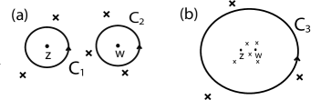
Figure 1: Schematic drawing of contours around which $y$ is taken. The crosses depict off-particle zeros. (a) $y$ is taken around $C_{1}$ and then $C_{2}$, not enclosing any off-particle zeros. The correlation function picks up a phase $2\pi(p_{\gamma+a;b}+p_{\gamma^{\prime}+c;b})$. (b) $z$ and $w$ are brought together, fusing $V_{\gamma+a}(z)$ and $V_{\gamma^{\prime}+c}(w)$, dragging in some of the off-particle zeros along with them. $y$ is taken around the fused combination, as illustrated by the contour $C_{3}$. The correlation function picks up a phase $2\pi p_{\gamma^{\prime\prime}+a+c;b}\geq 2\pi(p_{\gamma+a;b}+p_{\gamma^{\prime}+c;b})$.

Let us now look for such a condition. Suppose two quasiparticle operators $\gamma$ and $\gamma^{\prime}$ can fuse to a third one, $\gamma^{\prime\prime}$, and consider the OPE between the following three operators:

$$V_{\gamma+a}(z)V_{\gamma^{\prime}+c}(w)V_{b}(y)\sim f(z,w,y)V_{\gamma^{\prime\prime}+a+b+c}(z)+...$$ (45)

(Such an OPE makes sense if we are imagining a correlation function with all other operators inserted at points far away from $z$, $w$, and $y$.) Let us first fix all positions except $y$ and regard the correlation function as a function of $y$. Zeros (poles) of the correlation function can occur when $y$ coincides with the positions at which other operators are inserted. However zeros can also occur at locations away from the particles (see Figure 1). Imagine that we take $y$ around $w$ without enclosing any of the off-particle zeros. The phase that the correlation function acquires upon such a monodromy is simply $2\pi p_{\gamma^{\prime}+c;b}$. In terms of the scaling dimensions, the integer $p_{\gamma;b}$ is given by

$$p_{\gamma;b}=h_{\gamma+b}-h_{\gamma}-h_{b}=p_{\gamma;b}^{\text{sc}}+bQ_{\gamma}/\nu,$$ (46)

where

$$p_{\gamma;b}^{\text{sc}}=h_{\gamma+b}^{\text{sc}}-h_{\gamma}^{\text{sc}}-h_{b}^{\text{sc}}=\sum_{a=1}^{b}(l^{\text{sc}}_{\gamma;a}-l^{\text{sc}}_{a}).$$ (47)

If we take $y$ around $z$ without enclosing any off-particle zeros, the correlation function acquires a phase $2\pi p_{\gamma+a;b}$. Taking $y$ around $w$ and then around $z$ thus gives a total phase of $2\pi(p_{\gamma+a;b}+p_{\gamma^{\prime}+c;b})$. Compare that combined process with the following process: fuse $V_{\gamma+a}$ and $V_{\gamma^{\prime}+c}$ to get $V_{\gamma^{\prime\prime}+a+c}$, and take $V_{b}(y)$ around $V_{\gamma^{\prime\prime}+a+c}$; physically this corresponds to taking $z$ to be close to $w$ compared to $y$ and taking $y$ around a contour that encloses both $z$ and $w$ (Figure 1). The result of such an operation is that the correlation function acquires a phase of $2\pi p_{\gamma^{\prime\prime}+a+c;b}$. In fusing $V_{\gamma+a}(z)$ and $V_{\gamma^{\prime}+c}(w)$ to get $V_{\gamma^{\prime\prime}+a+c}(z)$, some of the off-particle zeros that were present before the fusion may now be located at $z$. That is, fusing $V_{\gamma+a}(z)$ and $V_{\gamma^{\prime}+c}(w)$ corresponds to taking $w\rightarrow z$, which in the process may take some of the off-particle zeros to $z$ as well. Therefore we can conclude:

$$p_{\gamma+a;b}+p_{\gamma^{\prime}+c;b}\leq p_{\gamma^{\prime\prime}+a+c;b},$$ (48)

which must be satisfied for all positive integers $a$, $b$, and $c$. The inequality is saturated when there are no off-particle zeros at all.

The $U(1)$ Abelian fusion rules imply charge conservation: $Q_{\gamma}+Q_{\gamma^{\prime}}=Q_{\gamma^{\prime\prime}}$, which means that the $U(1)$ part saturates the inequality (48) (see eqn. (46)). This allows us to obtain a more restrictive condition

$$p_{\gamma+a;b}^{\text{sc}}+p_{\gamma^{\prime}+c;b}^{\text{sc}}\leq p_{\gamma^{\prime\prime}+a+c;b}^{\text{sc}}$$ (49)

which corresponds to (48) applied to the simple current part. In terms of the sequences $\{l_{\gamma;a}\}$, the condition (49) becomes

$$\sum_{j=1}^{b}(l^{\text{sc}}_{\gamma+a;j}+l^{\text{sc}}_{\gamma^{\prime}+c;j}-l^{\text{sc}}_{j})\leq\sum_{j=1}^{b}l^{\text{sc}}_{\gamma^{\prime\prime}+a+c;j}$$ (50)

Remember that $l^{\text{sc}}_{\gamma;a}$ is obtained from $l_{\gamma;a}$ through eqn. (23) and eqn. (21). The pattern-of-zero sequences $\{l_{\gamma;a}\}$ that describe valid quasiparticles are solved from eqn. (13).

For states that satisfy the $n$-cluster condition, the scaling dimensions and hence the pattern of zeros have a periodicity of $n$:

$$p_{\gamma+a+n;b}^{\text{sc}}=p_{\gamma+a;b}^{\text{sc}}=p_{\gamma+a;b+n}^{\text{sc}}.$$ (51)

Therefore, $a$, $b$, and $c$ need only run through the values $0,...,n-1$.

The eqn. (49) or eqn. (50) is the condition that we are looking for. The fusion coefficient $N_{\gamma\gamma^{\prime}}^{\gamma^{\prime\prime}}$ can be non-zero only if the triplet $(\gamma,\gamma^{\prime},\gamma^{\prime\prime})$ conserves charge, $Q_{\gamma}+Q_{\gamma^{\prime}}=Q_{\gamma^{\prime\prime}}$, and satisfies eqn. (49) (or eqn. (50)) for any choice of $a,b,c$. This result allows us to calculate the fusion rules from the pattern of zeros.

Remarkably, the condition eqn. (49) or eqn. (50) appears to be complete enough. We find through numerical tests that for the generalized and composite parafermion states discussed below, condition (49) is sufficient to obtain the fusion rules: $V_{\gamma}$, $V_{\gamma^{\prime}}$, and $V_{\gamma^{\prime\prime}}$ satisfy (49) and charge conservation if and only if $V_{\gamma}$ and $V_{\gamma^{\prime}}$ can fuse to give $V_{\gamma^{\prime\prime}}$. We do not yet know, aside from these parafermion states, whether condition (49) is sufficient to obtain the fusion rules. If we assume $N_{\gamma\gamma^{\prime}}^{\gamma^{\prime\prime}}=0,1$, then it is possible that eqn. (49) or eqn. (50) completely determines the fusion rules.

III.4 Fusion Rules and Ground State Degeneracy on Genus $g$ Surfaces

After obtaining the fusion rules from the pattern of zeros (see eqn. (49)), we would like to ask: can we check this result physically, say through numerical calculations of some physical system? Given a pattern-of-zeros sequence, there is a local Hamiltonian, which was constructed in LABEL:WWsymm, whose ground state wave function is described by this pattern-of-zeros. The Hamiltonian can be solved numerically to obtain quasiparticle excitations and in principle we can check the the fusion rules. However, this approach does not really work since the numerical calculation will produce many quasiparticle excitations, and most of them only differ by local excitations and should be regarded as equivalent. We do not have a good way to determine which quasiparticles are equivalent and which are topologically distinct. This is why we cannot directly check the fusion rules of the excitations through numerical calculations.

However, there is an indirect way to check the fusion rules. The fusion rules in a topological phase also determine the ground state degeneracy on genus $g$ surfaces. We can numerically compute the ground state degeneracy on a genus $g$ surface and compare it with the result from the fusion rules.

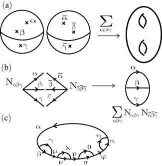
Figure 2: (a) Genus $g$ surfaces can be constructed by sewing together 3-punctured spheres; the case $g=2$ is shown here. (b) 3-punctured spheres can be depicted by vertices of $\varphi^{3}$ diagrams. There is a factor of $N_{\alpha\beta\gamma}$ for each vertex with outward directed edges $\alpha$, $\beta$, and $\gamma$. Reversing the direction of an edge corresponds to replacing a quasiparticle with its conjugate. The $g=2$ case is depicted by a 2-loop diagram, and has a factor $\sum_{\alpha\beta\gamma}N_{\alpha\beta\gamma}N_{\bar{\alpha}\bar{\beta}\bar{\gamma}}$. (c) An example of a 5-loop diagram, corresponding to a genus $g=5$ surface. This would give a factor $\sum N_{\bar{\alpha}\beta\gamma}N_{\bar{\beta}\bar{\gamma}\mu}N_{\bar{\mu}\nu\lambda}N_{\bar{\lambda}\bar{\nu}\rho}N_{\bar{\rho}\theta\sigma}N_{\bar{\theta}\bar{\sigma}\varphi}N_{\bar{\varphi}\eta\kappa}N_{\bar{\kappa}\bar{\eta}\alpha}$, which can be written more compactly as $\text{Tr}\left(\sum_{\alpha}N_{\alpha}N_{\bar{\alpha}}\right)^{g-1}$.

Why do fusion rules determine the ground state degeneracy? This is because genus $g$ surfaces may be constructed by sewing together 3-punctured spheres (see Fig. 2). Each puncture is labeled by a quasiparticle type, and two punctures can be sewed together by summing over intermediate states at the punctures. This corresponds to labeling one puncture by a quasiparticle $\gamma$, labeling the other puncture by the conjugate of $\gamma$, which is referred to as $\bar{\gamma}$, and summing over $\gamma$. $\bar{\gamma}$ is the unique quasiparticle that satisfies $N_{\gamma\bar{\gamma}}^{0}=1$; the operator that takes $\gamma$ to $\bar{\gamma}$ is the charge conjugation operator $C$: $C_{\alpha\beta}=N_{\alpha\beta}^{0}$. The dimension of the space of states of a 3-punctured sphere labeled by $\alpha$, $\beta$, and $\gamma$ is $N_{\alpha\beta\gamma}=N_{\alpha\beta}^{\bar{\gamma}}$. $N_{\alpha\beta\gamma}$ is symmetric in its indices, which we can raise and lower with the charge conjugation operator:

$$N_{\alpha\beta\gamma}=C_{\gamma\delta}N_{\alpha\beta}^{\delta}=N_{\alpha\beta}^{\bar{\gamma}}=C^{\bar{\gamma}\delta}N_{\alpha\beta\delta}.$$

$C^{\alpha\beta}$ is the inverse of $C_{\alpha\beta}$: $C^{\alpha\beta}C_{\beta\gamma}=\delta^{\alpha}_{\gamma}$. Also, note that $C$ squares to the identity, $C_{\alpha\beta}C_{\beta\gamma}=\delta_{\alpha\gamma}$, so that $C$ is its own inverse: $C_{\alpha\beta}=C^{\alpha\beta}$. If we represent a 3-punctured sphere by a vertex in a $\varphi^{3}$ diagram with directed edges and label the outgoing edges by $\alpha$, $\beta$, and $\gamma$, each vertex comes with a factor $N_{\alpha\beta\gamma}$. A genus $g$ surface can then be thought of as a $g$-loop diagram. This implies that the ground state degeneracy on a torus, for example, is $\sum_{\alpha,\beta}N_{0\alpha\beta}N_{0\bar{\alpha}\bar{\beta}}$. The ground state degeneracy on a genus 2 surface would be given by

$$\sum_{\alpha\beta\gamma}N_{\alpha\beta\gamma}N_{\bar{\alpha}\bar{\beta}\bar{\gamma}}=\sum_{\alpha\beta\gamma}N_{\alpha\beta}^{\gamma}N_{\bar{\alpha}\gamma}^{\beta}.$$

In general, one obtains the following formula for the ground state degeneracy in terms of the fusion rulesVerlinde (1988) (see Figure 2):

$$\text{ G.S.D. }=\text{Tr}\left(\sum_{a=0}^{N-1}N_{\alpha}N_{\bar{\alpha}}\right)^{g-1}.$$ (52)

$N$ is the number of quasiparticle types, $(N_{\alpha})_{\beta}^{\gamma}=N_{\alpha\beta}^{\gamma}$, and matrix multiplication of the fusion matrices is defined by contracting indices, so that $(N_{\alpha}N_{\beta})_{i}^{j}=N_{\alpha i}^{k}N_{\beta k}^{j}$. (52) assumes that all fields are fusing to the identity, so it applies only when the total number of electrons is a multiple of $n$ (for $n$-cluster states). For other cases, one must perform a more careful analysis.

We show in Appendix B that (52) can be rewritten as

$$\text{G.S.D.}=\left(\sum_{\gamma=0}d_{\gamma}^{2}\right)^{g-1}\sum_{\gamma=0}^{N-1}d_{\gamma}^{-2(g-1)}.$$ (53)

$d_{\gamma}$ is the “quantum dimension” of quasiparticle $\gamma$. It is given by the largest eigenvalue of the fusion matrix $N_{\gamma}$, and it has the property that the space of states with $n$ quasiparticles of type $\gamma$ at fixed locations goes as $\sim d_{\gamma}^{n}$ for large $n$. In particular, Abelian quasiparticles have unit quantum dimension. It is remarkable that the ground state degeneracy on any surface is determined solely by the quantum dimensions of quasiparticles.

From (53) and the magnetic algebra structure of the quasiparticles, we can prove that the ground state degeneracy on genus $g$ surfaces factorizes into a part that depends only on the filling fraction $\nu$ and a part that depends only on the simple current CFT. In particular, we show in Appendix B that (53) can be rewritten as

G.S.D. $$=\nu^{-g}\left(\sum_{i}c_{i}^{\text{sc}}d_{i}^{2}\right)^{g-1}\left(\sum_{i}c_{i}^{\text{sc}}d_{i}^{-2(g-1)}\right).$$ (54)

Here $\sum_{i}$ sums over the representations (which are labeled by $i$) of the magnetic translation algebra. $d_{i}$ is the quantum dimension of quasiparticles in the $i^{th}$ representation. $c_{i}^{\text{sc}}$ is the number of distinct fields of the form $\psi^{a}\sigma_{i}$ for a fixed $i$. It can be determined from the pattern-of-zeros as follows. Recall that all of the quasiparticles in the $i^{\text{th}}$ representation of the magnetic translation algebra have the same sequence $\{l^{\text{sc}}_{i;a}\}$ up to a cyclic permutation. $c_{i}^{\text{sc}}$ describes the shortest period of $\{l^{\text{sc}}_{i;a}\}$:

$$l^{\text{sc}}_{i;a}=l^{\text{sc}}_{i;a+c_{i}^{\text{sc}}}.$$

$\{l^{\text{sc}}_{i;a}\}$ always satisfies $l^{\text{sc}}_{i;a}=l^{\text{sc}}_{i;a+n}$ and very often $c_{i}^{\text{sc}}=n$. But sometimes, $c_{i}^{\text{sc}}$ can be a factor of $n$.

We see that the $c_{i}^{\text{sc}}$ are determined from the pattern of zeros of the quasiparticles. We have seen that (under certain assumptions) the fusion rules (and hence the quantum dimensions $d_{i}$) can also be determined from the pattern of zeros. Thus eqn. (54) allows us to calculate the ground state degeneracy on any genus $g$ surface from the pattern of zeros.

(54) shows that the ground state degeneracy on a genus $g$ surface factorizes into $\nu^{-g}$ times a factor that depends only on the simple current CFT. This is remarkable because $\nu^{-1}$ is generically not an integer. The second factor may be interpreted as the dimension of the space of conformal blocks on a genus $g$ surface with no punctures for the simple current CFT. In particular, for genus one, this gives $1/\nu$ times the number of distinct fields of the form $\psi^{a}\sigma_{i}$ in the simple current CFT, a result which we find more explicitly in the following section for the parafermion quantum Hall states. Note that this formula assumes that the number of electrons is a multiple of $n$; we expect a similar decomposition into $\nu^{-g}$ times a factor that depends only on the simple current CFT if the electron number is not a multiple of $n$, but we will not analyze here this more complicated case.

IV Parafermion Quantum Hall States

Using the pattern-of-zero approach, we can obtain the number of types of quasiparticles,Wen and Wang (2008a, b) the fusion rules, etc . However, to obtain those results from the pattern-of-zero approach, we have made certain assumptions. In this section, we will study some FQH states using the CFT approach to confirm those results obtained from the pattern-of-zero approach.

The quantum Hall states to which we now turn include the parafermionRead and Rezayi (1999), “generalized parafermion,” and “composite parafermion” Wen and Wang (2008a) states. These states are all based on the $Z_{n}$ parafermion conformal field theory introduced by Zamolodchikov and FateevZamolodchikov and Fateev (1985). In the context of quantum Hall states, we focus on the holomorphic part of the theory and leave out the anti-holomorphic part. The $Z_{n}$ parafermion CFT is generated by $n$ simple currents $\psi_{a}(z)$, $a=0,...,n-1$, which have a $Z_{n}$ symmetry: $\psi_{1}^{n}=1$ and $\psi_{a}=\psi_{1}^{a}$.

The field space of the theory splits into a direct sum of subspaces, each with a certain $Z_{n}$ charge, labeled by $l$, with $l=0,..,n-1$. The fields with minimal scaling dimension in each of these subspaces are the so-called “spin fields” or “disorder operators” $\sigma_{l}$. Fields in each subspace are generated from the $\sigma_{l}$ by acting with the simple currents: $\psi_{a}\sigma_{l}$. Based on a relation between $SU(2)$ current algebra and parafermion theory, a way of labeling these primary fields is as $\Phi^{l}_{m}$.Gepner and Qiu (1987) The spin fields are $\sigma_{l}=\Phi^{l}_{l}$ and the simple currents are $\psi_{a}=\Phi^{0}_{2a}$. The $Z_{n}$ symmetry implies that $\Phi^{l}_{m+2n}=\psi_{1}^{n}\Phi^{l}_{m}=\Phi^{l}_{m}$. The scaling dimensions of the simple currents $\psi_{a}=\Phi^{0}_{2a}$ are chosen to be

$$\Delta^{0}_{2a}=\frac{a(n-a)}{n}.$$ (55)

Such a choice then determines the scaling dimensions of the rest of the fields in the theory. The scaling dimension $\Delta^{l}_{m}$ of the field $\Phi^{l}_{m}$ is given by

$$\Delta^{l}_{m}=\left\{\begin{array}[]{lll}\frac{l(l+2)}{4(n+2)}-\frac{m^{2}}{4n}+\frac{m-l}{2}&\mbox{ if }&l\leq m\leq 2n-l\\ \frac{l(l+2)}{4(n+2)}-\frac{m^{2}}{4n}&\mbox{ if }&-l\leq m\leq l\\ \end{array}\right.$$ (56)

$l$ and $m$ satisfy

$$l+m=\text{even},\ \ \ \ \ 0\leq l\leq n.$$ (57)

In the $\widehat{su}(2)_{n}/\widehat{u}(1)$ coset formulation of the parafermion CFTs, the following field identifications are made:

$$\{l,m\}\sim\{n-l,m-n\}\sim\{n-l,n+m\}.$$ (58)

Also, the $Z_{n}$ structure implies:

$$\{l,m\}\sim\{l,m+2n\}.$$ (59)

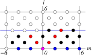
Figure 3: (Color online) The filled dots represent the distinct $\Phi^{l}_{m}$’s in $Z_{6}$ parafermion CFT. The blue dots represent the simple current operators $\Phi^{0}_{2a}=\psi_{a}$ and the red dots represent the spin operators $\Phi^{l}_{l}=\sigma_{l}$.

From (57), (58), and (59), we can find the distinct $\Phi^{l}_{m}$’s (see Fig. 3). In the pattern-of-zero picture, the identification (58) is natural because quasiparticles containing the field $\Phi^{l}_{m}$ yield the same pattern of zeros as those containing the field $\Phi^{n-l}_{n+m}$ and for this reason are considered to be physically equivalent.

The electron operator in the conventional Read-Rezayi $Z_{n}$ parafermion quantum Hall states at filling fraction $\nu$ is given by

$$V_{\text{e}}(z)=\psi_{1}(z)\hskip 1.0pt\mathrm{e}^{\hskip 1.0pt\mathrm{i}\hskip 1.0pt\sqrt{\frac{1}{\nu}}\varphi(z)}.$$ (60)

In the “generalized” $Z_{n}^{(k)}$ parafermion states, we use $\psi_{k}$ instead of $\psi_{1}$ to define the electron operator:

$$V_{\text{e}}(z)=\psi_{k}(z)\hskip 1.0pt\mathrm{e}^{\hskip 1.0pt\mathrm{i}\hskip 1.0pt\sqrt{\frac{1}{\nu}}\varphi(z)}.$$ (61)

The states $Z_{n}^{(1)}$ thus correspond to the conventional Read-Rezayi states. The condition that the electron operator have integer or half-integer spin translates into a discrete set of possible filling fractions for the $Z_{n}^{(k)}$ parafermion states:

$$\nu=\frac{n}{nM+2k^{2}}$$ (62)

$M$ is a nonnegative integer; that it must be nonnegative is derived from the condition that the operator product expansion (OPE) between two electrons must not diverge as two electrons are brought close to each other. Eqn. (62) is the generalization of the well-known formula $\nu=\frac{n}{nM+2}$ for the conventional $Z_{n}$ Read-Rezayi parafermion states. In what follows, we assume $k$ and $n$ are coprime; cases in which they are not must be treated differently.

The quasiparticle fields take the form

$$V_{\gamma}=\Phi^{l}_{m}\hskip 1.0pt\mathrm{e}^{\hskip 1.0pt\mathrm{i}\hskip 1.0ptQ_{\gamma}\sqrt{\frac{1}{\nu}}\varphi},$$ (63)

where $Q_{\gamma}$ is the electric charge of the quasiparticle. $V_{\gamma}$ is a valid quasiparticle if and only if it has a single-valued OPE with the electron operator. To find the number of distinct quasiparticle types, we need to find all the valid quasiparticle operators $V_{\gamma}$ while regarding two quasiparticle operators as equivalent if they differ by an electron operator.

Since quasiparticle operators that differ by an electron operator are regarded as equivalent, every quasiparticle is equivalent to one whose charge lies between $0$ and $1$. Thus a simple way of dealing with this equivalence relation is to restrict ourselves to considering operators whose charges $Q_{\gamma}$ satisfy

$$0\leq Q_{\gamma}<1.$$ (64)

This ensures that we consider a single member of each equivalence class, because adding an electron to a quasiparticle operator increases its charge by one. For each primary field labeled by $\{l,m\}$, there are only a few choices of $Q_{\gamma}$ that satisfy eqn. (64) and that will make the operator $V_{\gamma}$ local with respect to the electron operator. Finding all these different allowed charges for each $\{l,m\}$ will give us all the different quasiparticle types.

The OPE between the quasiparticle operator and the electron is

$$V_{\gamma}(z)V_{\text{e}}(w)\sim(z-w)^{a}\Phi^{l}_{m+2k}\hskip 1.0pt\mathrm{e}^{\hskip 1.0pt\mathrm{i}\hskip 1.0pt(Q_{\gamma}+1)\frac{1}{\sqrt{\nu}}\varphi},$$ (65)

$$a=\Delta^{l}_{m+2k}-\Delta^{l}_{m}-\Delta^{0}_{2k}+Q_{\gamma}/\nu.$$ (66)

Locality (single-valuedness) between the quasiparticle and the electron implies that $a$ must be an integer. Each allowed charge $Q_{\gamma}$ for a given primary field $\{l,m\}$ can therefore be labeled by an integer $a$ that, from eqn. (64), satisfies

$$0\leq a-\Delta^{l}_{m+2k}+\Delta^{l}_{m}+\Delta^{0}_{2k}<1/\nu.$$ (67)

Therefore, to find all the distinct, valid quasiparticles, we search through all of the distinct, allowed triplets $\{a,l,m\}$, subject to (57) and the identifications in (58) and (59), and find those that satisfy eqn. (67). Carrying out this program on a computer, we learn that the number of quasiparticles in the generalized $Z_{n}^{(k)}$ parafermion states follows the formula

$$\mbox{ No. of Quasiparticles }=\frac{1}{2}\frac{n(n+1)}{\nu}.$$ (68)

This is the natural generalization of the formula $\frac{1}{2}(nM+2)(n+1)$ that is well-known for the $k=1$ case.

The pattern-of-zeros approach has yielded not only these generalized parafermion states, but also a series of “composite parafermion” states. In these states, the relevant conformal field theory is chosen to consist of several parafermion conformal field theories taken together, of the form $\bigotimes_{i}Z_{n_{i}}^{(k_{i})}$. We emphasize that here the $n_{i}$ are all coprime with respect to one another and $k_{i}$ is coprime with respect to $n_{i}$. Cases in which these coprime conditions do not hold should be treated differently. Here, the electron operator is

$$V_{\text{e}}=\prod_{i=1}\psi_{k_{i};n_{i}}\hskip 1.0pt\mathrm{e}^{\hskip 1.0pt\mathrm{i}\hskip 1.0pt\sqrt{\frac{1}{\nu}}\varphi},$$ (69)

where $\psi_{k_{i};n_{i}}$ is a simple current of the $Z_{n_{i}}$ parafermion CFT. The condition for the filling fraction, eqn. (62), generalizes to

$$\nu=\frac{N}{NM+2N\sum_{i}\frac{k_{i}^{2}}{ni}},$$ (70)

where $N=\prod_{i}n_{i}$ and $M$ is a nonnegative integer. Following a procedure similar to that described above in the generalized parafermion case, the condition eqn. (67) generalizes to

$$0\leq a-\sum_{i}(\Delta^{l_{i}}_{m_{i}+2k_{i};n_{i}}+\Delta^{l_{i}}_{m_{i};n_{i}}+\Delta^{0}_{2k_{i};n_{i}})<1/\nu$$ (71)

where $\Delta^{l_{i}}_{m_{i};n_{i}}$ is the scaling dimension $\Delta^{l_{i}}_{m_{i}}$ from the $Z_{n_{i}}$ parafermion CFT. We find that the number of quasiparticles follows the natural generalization of eqn. (68):

$$\mbox{ No. of Quasiparticles }=\frac{1}{\nu}\prod_{i}\frac{n_{i}(n_{i}+1)}{2}$$ (72)

Strikingly, these results agree with the number of quasiparticles computed in an entirely different fashion through the pattern-of-zero approach.Wen and Wang (2008b)

Since we know the fusion rules in the $Z_{n}$ parafermion CFTs, we can easily examine the fusion rules in the parafermion quantum Hall states. The most general states that we have discussed in this section have been the $\bigotimes_{i}Z_{n_{i}}^{(k_{i})}$ composite parafermion states. The quasiparticles operators can be written as

$$V_{\gamma}=\prod_{i=1}\Phi^{l_{i}}_{m_{i};n_{i}}\hskip 1.0pt\mathrm{e}^{\hskip 1.0pt\mathrm{i}\hskip 1.0pt\sqrt{Q_{\gamma}\frac{1}{\nu}}\varphi},$$ (73)

where $\Phi^{l_{i}}_{m_{i};n_{i}}$ is the primary field $\Phi^{l_{i}}_{m_{i}}$ from the $Z_{n_{i}}$ parafermion CFT. Equivalently, we can label each quasiparticle as $\{Q_{\gamma};l_{1},m_{1},l_{2},m_{2},\cdots\}$.

The primary fields $\Phi^{l}_{m}$ in the $Z_{n}$ parafermion CFT enjoy the following fusion rulesGepner and Qiu (1987):

$$\Phi^{l}_{m}\times\Phi^{l^{\prime}}_{m^{\prime}}=\sum_{j=\mid l-l^{\prime}\mid}^{min(l+l^{\prime},n-l-l^{\prime})}\Phi^{j}_{m+m^{\prime}}.$$ (74)

Therefore, in terms of the $\{Q_{\gamma};l_{1},m_{1},\cdots\}$ labels, the fusion rules for the quasiparticles in the composite parafermion states are given by

$$\{Q_{\gamma};l_{1},m_{1},\cdots\}\times\{Q_{\gamma^{\prime}};l^{\prime}_{1},m^{\prime}_{1},\cdots\}=\sum_{l^{\prime\prime}_{i}=\mid l_{i}-l_{i}^{\prime}\mid}^{min(l_{i}+l_{i}^{\prime},n_{i}-l_{i}-l_{i}^{\prime})}\{Q_{\gamma}+Q_{\gamma^{\prime}};l^{\prime\prime}_{1},m_{1}+m^{\prime}_{1},l_{2}^{\prime\prime},m_{2}+m_{2}^{\prime},\cdots\},$$ (75)

where there is a sum over each $l_{i}^{\prime\prime}$ for $i=1,2,\cdots$, and we make the identifications

$$\{Q_{\gamma};\cdots,l_{i},m_{i},\cdots\} \sim\{Q_{\gamma};\cdots,n_{i}-l_{i},m_{i}-n_{i},\cdots\}$$

$$\sim\{Q_{\gamma};\cdots,l_{i},m_{i}+2n_{i},\cdots\}\sim\{Q_{\gamma}+1;\cdots,l_{i},m_{i}+2k_{i},\cdots\}.$$ (76)

Such a fusion rule agrees with that obtained previously from the pattern of zeros.

V Examples

$Z_{3}^{(1)}$ $\nu=3/2$
$\{Q_{\gamma};l,m\}$	$\{n_{\gamma;l}\}$	$n\cdot\{\tilde{l}_{\gamma;a}^{sc}\}$	$h_{\gamma}$	$h_{\gamma}^{sc}$	$h_{\gamma,min}^{sc}$
{0; 0, 0}	30	2 0 -2	0	0	0
{1/2; 0, -2}	03	-2 2 0	3/4	2/3	0
{1/2; 1, 1}	21	1 -1 0	3/20	1/15	1/15
{0; 1, 3}	12	-1 0 1	2/15	2/5	1/15

Table 2: Pattern-of-zeros, scaling dimensions, and charges for the quasiparticles in $Z_{3}^{(1)}$ at $\nu=3/2$. The periodic sequence $\tilde{l}_{\gamma;a}^{sc}$ is listed for $a=1,\cdots,3$. The asymptotic form of a single unit cell of $\{n_{\gamma;l}\}$ is shown.

$Z_{5}^{(1)}$ $\nu=5/2$
$\{Q_{\gamma};l,m\}$	$\{n_{\gamma;l}\}$	$n\cdot\{\tilde{l}_{\gamma;a}^{sc}\}$	$h_{\gamma}$	$h_{\gamma}^{sc}$	$h_{\gamma,min}^{sc}$
$\{1/2;0,6\}$	05	-2 -4 4 2 0	$\frac{5}{4}$	$\frac{6}{5}$	0
$\{0;0,0\}$	50	4 2 0 -2 -4	0	0	0
$\{1/2;1,1\}$	41	3 1 -1 -3 0	$\frac{3}{28}$	$\frac{2}{35}$	$\frac{2}{35}$
$\{0;1,5\}$	14	-1 -3 0 3 1	$\frac{6}{7}$	$\frac{6}{7}$	$\frac{2}{35}$
$\{1/2;2,6\}$	23	-2 1 -1 2 0	$\frac{15}{28}$	$\frac{17}{35}$	$\frac{3}{35}$
$\{0;2,0\}$	32	-1 2 0 -2 1	$\frac{2}{7}$	$\frac{2}{7}$	$\frac{3}{35}$

Table 3: Pattern-of-zeros, scaling dimensions, and charges for the quasiparticles in $Z_{5}^{(1)}$ at $\nu=5/2$. The periodic sequence $\tilde{l}_{\gamma;a}^{sc}$ is listed for $a=1,\cdots,5$. The asymptotic form of a single unit cell of $\{n_{\gamma;l}\}$ is shown.

$Z_{5}^{(2)}$ $\nu=5/8$
$\{Q_{\gamma};l,m\}$	$\{n_{\gamma;l}\}$	$n\cdot\{\tilde{l}_{\gamma;a}^{sc}\}$	$h_{\gamma}$	$h_{\gamma}^{sc}$	$h_{\gamma,min}^{sc}$
$\{0;0,0\}$	20102000	6 -2 0 2 -6	0	0	0
$\{5/8;0,0\}$	02010200	6 -2 0 2 -6	$\frac{5}{16}$	0	0
$\{2/8;0,6\}$	00201020	-6 6 -2 0 2	$\frac{5}{4}$	$\frac{6}{5}$	0
$\{7/8;0,6\}$	00020102	-6 6 -2 0 2	$\frac{29}{16}$	$\frac{6}{5}$	0
$\{4/8;0,2\}$	20002010	2 -6 6 -2 0	1	$\frac{4}{5}$	0
$\{1/8;0,8\}$	02000201	0 2 -6 6 -2	$\frac{13}{16}$	$\frac{4}{5}$	0
$\{6/8;0,8\}$	10200020	0 2 -6 6 -2	$\frac{5}{4}$	$\frac{4}{5}$	0
$\{3/8;0,4\}$	01020002	-2 0 2 -6 6	$\frac{21}{16}$	$\frac{6}{5}$	0
$\{0;1,5\}$	01110020	-4 3 0 -3 4	$\frac{6}{7}$	$\frac{6}{7}$	$\frac{2}{35}$
$\{5/8;1,5\}$	00111002	-4 3 0 -3 4	$\frac{131}{112}$	$\frac{6}{7}$	$\frac{2}{35}$
$\{2/8;1,1\}$	20011100	4 -4 3 0 -3	$\frac{3}{28}$	$\frac{2}{35}$	$\frac{2}{35}$
$\{7/8;1,1\}$	02001110	4 -4 3 0 -3	$\frac{75}{112}$	$\frac{2}{35}$	$\frac{2}{35}$
$\{4/8;1,7\}$	00200111	-3 4 -4 3 0	$\frac{6}{7}$	$\frac{23}{35}$	$\frac{2}{35}$
$\{1/8;1,3\}$	10020011	0 -3 4 -4 3	$\frac{75}{112}$	$\frac{23}{35}$	$\frac{2}{35}$
$\{6/8;1,3\}$	11002001	0 -3 4 -4 3	$\frac{31}{28}$	$\frac{23}{35}$	$\frac{2}{35}$
$\{3/8;1,-1\}$	11100200	3 0 -3 4 -4	$\frac{19}{112}$	$\frac{2}{35}$	$\frac{2}{35}$
$\{0;2,0\}$	10101101	1 -2 0 2 -1	$\frac{2}{7}$	$\frac{2}{7}$	$\frac{3}{35}$
$\{5/8;2,0\}$	11010110	1 -2 0 2 -1	$\frac{67}{112}$	$\frac{2}{7}$	$\frac{3}{35}$
$\{2/8;2,6\}$	01101011	-1 1 -2 0 2	$\frac{15}{28}$	$\frac{17}{35}$	$\frac{3}{35}$
$\{7/8;2,6\}$	10110101	-1 1 -2 0 2	$\frac{615}{560}$	$\frac{17}{35}$	$\frac{3}{35}$
$\{4/8;2,2\}$	11011010	2 -1 1 -2 0	$\frac{2}{7}$	$\frac{3}{35}$	$\frac{3}{35}$
$\{1/8;2,-2\}$	01101101	0 2 -1 1 -2	$\frac{11}{112}$	$\frac{3}{35}$	$\frac{3}{35}$
$\{6/8;2,-2\}$	10110110	0 2 -1 1 -2	$\frac{15}{28}$	$\frac{3}{35}$	$\frac{3}{35}$
$\{3/8;2,4\}$	01011011	-2 0 2 -1 1	$\frac{67}{112}$	$\frac{17}{35}$	$\frac{3}{35}$

Table 4: Pattern-of-zeros, scaling dimensions, and charges for the quasiparticles in $Z_{5}^{(2)}$ at $\nu=5/8$. The periodic sequence $\tilde{l}_{\gamma;a}^{sc}$ is listed for $a=1,\cdots,5$. The asymptotic form of a single unit cell of $\{n_{\gamma;l}\}$ is shown. Note that the charges, modulo one, of two quasiparticles that are related by a translation $\hat{T}_{1}$ differ by $\nu=5/8$, as explained in Section III.2.

Now we will describe some specific examples of the parafermion states, listing their pattern-of-zeros, scaling dimensions, ground state degeneracies, and discussing their fusion rules.

In the $Z_{3}^{(1)}$ state at $\nu=3/2$ (which is the bosonic $Z_{3}$ parafermion stateRead and Rezayi (1999)), Table 2 shows that there are two representations of the magnetic algebra, with two quasiparticles in each representation. These two representations are irreducible ($q=m$), so the fusion rules decompose as (39). Labeling these two by $1$ (the identity) and $\sigma$, we see that they satisfy the fusion rules

$$\sigma\sigma=1+\sigma.$$ (77)

There are only two modular tensor categories of rank 2, the so-called semion MTC and the Fibonacci MTC, and we see that these fusion rules correspond to the Fibonacci MTC.Rowell et al. (2007)

In the $Z_{5}^{(k)}$ statesWen and Wang (2008a), we also have $q=m$ and the quasiparticles form three irreducible representations of the magnetic algebra. The fusion algebra again has the simple decomposition eqn. (39). In the $Z_{5}^{(1)}$ state at $\nu=5/2$, Table 3 shows that there are two quasiparticles in each irreducible representation, while in the $Z_{5}^{(2)}$ state at $\nu=5/8$, Table 4 shows that there are eight quasiparticles in each irreducible representation of the magnetic algebra. The non-trivial, non-Abelian part of the fusion rules is given by the fusion rules among the three irreducible representations. Labeling these three by $1$, $\sigma_{1}$, and $\sigma_{2}$, and using eqn. (49) or eqn. (75), we can see that they satisfy the following fusion rules:

$$\sigma_{1}\sigma_{1}=1+\sigma_{2},$$

$$\sigma_{2}\sigma_{2}=1+\sigma_{1}+\sigma_{2},$$

$$\sigma_{1}\sigma_{2}=\sigma_{1}+\sigma_{2}.$$ (78)

This corresponds to the $(A_{1},5)_{\frac{1}{2}}$ MTC described in LABEL:RSW0777.

We see that when $q=m$, the decomposition of the fusion rules (39) into a non-trivial, non-Abelian part that depends only on how the different irreducible representations fuse together and a trivial Abelian part greatly simplifies these states. The $Z_{3}^{(1)}$ state, which at $\nu=3/2$ contains four quasiparticles, has only two irreducible representations of the magnetic algebra and therefore the non-Abelian part is described by a simple rank 2 modular tensor category (MTC)Rowell et al. (2007): the Fibonacci MTC. Similarly, $Z_{5}^{(k)}$, which for $k=2$ and $\nu=5/8$ has 24 quasiparticles, actually has only three different irreducible representations of the magnetic algebra, and therefore the non-Abelian part of its fusion rules is described by a simple rank 3 MTC. The $Z_{2}$ states listed previously in Table 1 have two representations, yet one of them is not irreducible. It turns out that the non-trivial, non-Abelian part of the fusion rules in the $Z_{2}$ states is described by the rank 3 Ising MTC. So, even though $Z_{5}^{(2)}$ at first sight seems a great deal more complicated than $Z_{2}$, their non-Abelian parts have the same degree of complexity, namely they are both described by a rank 3 MTC.

Using the fusion rules $(\ref{FRcft})$, we can also verify that the ground state degeneracy on genus $g$ surfaces follows the decomposition $(\ref{gsd})$. In particular, for the $Z_{n}$ parafermion CFTs of Zamolodchikov and Fateev, the quantum dimensions of the fields $\sigma_{l}\equiv\Phi^{l}_{l}$ can be found from the relation of these theories to $SU(2)_{k}$ WZW models.Francesco et al. (1997) The result is:

$$d_{l}=\frac{\sin(\frac{\pi(l+1)}{n+2})}{\sin(\frac{\pi}{n+2})}.$$ (79)

From the relations (58), it follows that for $n$ even, there are $\frac{n}{2}+1$ distinct $\sigma_{l}$’s. $c_{l}^{\text{sc}}=n$ for $l=0,\cdots,n/2-1$ and $c_{n/2}^{\text{sc}}=n/2$. For $n$ odd, there are $\frac{n+1}{2}$ distinct $\sigma_{l}$’s, and $c_{l}^{\text{sc}}=n$ for $l=0,\cdots,\frac{n-1}{2}$. Using $(\ref{gsd})$, we find that the ground state degeneracy for the $Z_{n}^{(k)}$ states on a genus $g$ surface is given by

$$\text{ G.S.D. }=\nu^{-g}n^{g}\times\left\{\begin{array}[]{lll}\left(\sum_{l=1}^{n/2}\sin^{2}(\frac{l\pi}{n+2})+\frac{1}{2}\right)^{g-1}\left(\sum_{l=1}^{n/2}\left(\sin(\frac{l\pi}{n+2})\right)^{-2(g-1)}+\frac{1}{2}\right)&\mbox{ if }&$n$\text{ is even }\\ \left(\sum_{l=1}^{(n+1)/2}\sin^{2}(\frac{l\pi}{n+2})\right)^{g-1}\left(\sum_{l=1}^{(n+1)/2}\left(\sin(\frac{l\pi}{n+2})\right)^{-2(g-1)}\right)&\mbox{ if }&$n$\text{ is odd }\\ \end{array}\right.$$ (80)

Table 5 lists the ground state degeneracies obtained from the above formula for the cases $n=2$,Oshikawa et al. (2007) 3, 4.Ardonne et al. (2008) These are the same results that one would obtain by numerically computing (52) for the fusion rules (75). For the $Z_{n}^{(1)}$ states, they also match the same results obtained in LABEL:ABK0816.

Ground State Degeneracies for $Z_{n}^{(k)}$ states
$n$	GSD
2	$\nu^{-g}2^{g-1}(2^{g}+1)$
3	$\nu^{-g}3^{g}(1+\varphi^{2})^{g-1}(1+\varphi^{-2(g-1)})$
4	$\nu^{-g}2^{g-1}(3^{g}+1+(2^{2g}-1)(3^{g-1}+1))$

Table 5: Ground State Degeneracies on genus $g$ surfaces for $Z_{n}^{(k)}$ parafermion quantum Hall states for the case when the number of electrons is a multiple of $n$. $\varphi=\frac{1+\sqrt{5}}{2}$ is the golden ratio.

VI Summary

Motivated by the characterization of symmetric polynomials and FQH states through the pattern of zeros,Wen and Wang (2008a) we examined the CFT generated by simple currents in terms of the pattern of zeros. This reveals a deep connection between the simple current CFT and FQH states. The point of view from the pattern of zeros reveals a magnetic translation algebra that acts on the quasiparticles. This allows us to greatly simplify the fusion algebra of the quasiparticles. It also allows us to show in general that the ground state degeneracy on genus $g$ surfaces is $\nu^{-g}$ times a factor that depends only on the simple current part of the CFT. More importantly, we are able to derive a necessary condition on the fusion rules of the quasiparticles based on the pattern of zeros. Such a necessary condition is sufficient to produce a full set of fusion rules for quasiparticles if we assume $N^{\gamma^{\prime\prime}}_{\gamma\gamma^{\prime}}=0,1$.

The results obtained from the pattern-of-zeros approach is checked against known results from the generalized and composite parafermion CFT. In particular, we find that the number of quasiparticles obtained from the pattern-of-zeros approachWen and Wang (2008b) agrees with that obtained from the CFT approach. The fusion rules obtained from the pattern of zeros also agrees with the result from the CFT calculation for generalized and composite parafermion FQH states. Those agreements further demonstrate that the pattern-of-zeros approach is quite a powerful tool to characterize and to calculate the topological properties of generic FQH states.

We would like to thank Zhenghan Wang for many helpful discussions. This research is supported by NSF Grant DMR-0706078.

Appendix A Scaling Dimensions of Quasiparticles

The way the magnetic algebra structure of the quasiparticles factorizes in the fusion rules is also seen in another topological property of the quasiparticles: the scaling dimensions, or spins, of the quasiparticles. Since quasiparticles that belong to the same representation of the magnetic algebra are described by sequences $\{l^{\text{sc}}_{\gamma;a}\}$ that are related by a cyclic permutation, from eqn. (25) we see that for each irreducible representation there is a single number $h_{\gamma;\text{min}}^{\text{sc}}$ that we need in order to calculate the scaling dimensions of all other quasiparticles in the same representation. $h_{\gamma;\text{min}}^{\text{sc}}$ is the minimum of $h_{\gamma+a}^{\text{sc}}$ over all the quasiparticles that belong to this representation. Given $h_{\gamma;\text{min}}^{\text{sc}}$, the scaling dimension of the quasiparticle $V_{\gamma+a}$ can be calculated from its pattern of zeros $\{\tilde{l}^{\text{sc}}_{\gamma+a;b}\}$.

It is not obvious that the information to obtain $h_{\gamma;\text{min}}^{\text{sc}}$ for each irreducible representation is even contained in the pattern of zeros. It may be that $\{l_{\gamma;a}\}$ is not enough information to uniquely specify the CFT and therefore also not enough information to completely determine the scaling dimensions of the fields that are contained in the theory. However, in the case where the pattern of zeros corresponds to the (generalized and composite) parafermion states discussed above, there are explicit formulas in terms of $l_{\gamma;a}$ that yield $h_{\gamma;\text{min}}^{\text{sc}}$. This comes as no surprise because in these cases, the pattern-of-zeros completely specifies the CFT. We do not have a formula that can even be applied in the more general situations.

Let us now describe how to calculate the scaling dimension $h_{\gamma+a}$ of the operator $V_{\gamma+a}$ given $h_{\gamma;\text{min}}^{\text{sc}}$. First we must find the index $a_{0}$ at which

$$h_{\gamma;\text{min}}^{\text{sc}}=h^{\text{sc}}_{\gamma+a+a_{0}}.$$ (81)

This is equivalent to finding the index $a_{0}$ at which

$$h_{\gamma+k}-h_{\gamma+a+a_{0}}\geq 0$$ (82)

for all $k$, because $h_{\gamma;\text{min}}^{\text{sc}}$ is defined to be the minimum of $h_{\gamma+k}$ over all $k$. Recalling that $\tilde{l}^{\text{sc}}_{\gamma+a;b+1}=h^{\text{sc}}_{\gamma+a+b+1}-h^{\text{sc}}_{\gamma+a+b}$, we see that $a_{0}$ is therefore the index at which

$$\sum_{i=1}^{k}\tilde{l}^{\text{sc}}_{\gamma+a;a_{0}+i} =h^{\text{sc}}_{\gamma+a+a_{0}+k}-h^{\text{sc}}_{\gamma+a+a_{0}}$$

$$=h^{\text{sc}}_{\gamma+a+a_{0}+k}-h^{\text{sc}}_{\gamma;\text{min}} \geq 0$$ (83)

for all $k$. Using eqn. (A), we can determine $a_{0}$ from $\{\tilde{l}^{\text{sc}}_{\gamma;a}\}$, after which we can determine $h_{\gamma+a}$ using eqn. (25):

$$h_{\gamma+a}^{\text{sc}}=h_{\gamma;\text{min}}^{\text{sc}}-\sum_{b=1}^{a_{0}}\tilde{l}^{\text{sc}}_{\gamma+a;b}.$$ (84)

Appendix B Ground State Degeneracy on Genus $g$ Surfaces

Here we illustrate how (53) and (54) can be determined from (52). First we observe that the fusion matrices $N_{\alpha}$ commute (and can therefore be simultaneously diagonalized) because the fusion of any three quasiparticles $\alpha$, $\beta$, and $\gamma$ should be independent of the order in which they are fused together. Remarkably, there is a symmetric unitary matrix $S$, known as the modular $S$ matrix, which squares to the charge conjugation operator, $S_{\alpha\beta}S_{\beta\gamma}=C_{\alpha\gamma}$, and that simultaneously diagonalizes all of the fusion matrices:Verlinde (1988); Moore and Seiberg (1988, 1989)

$$N_{\alpha\beta}^{\gamma}=\sum_{n}S_{\beta n}\lambda_{\alpha}^{(n)}S^{\dagger}_{\gamma n}.$$ (85)

Using (85) and the fact that $N_{\alpha 0}^{\beta}=\delta^{\beta}_{\alpha}$, the eigenvalues $\lambda_{\alpha}^{(n)}$ of the fusion matrix $N_{\alpha}$ can be written in terms of $S$:

$$\lambda_{\alpha}^{(n)}=\frac{S_{\alpha n}}{S_{0n}}.$$ (86)

$S$ also has the remarkable property that the largest eigenvalue of $N_{\alpha}$, which is the quantum dimension $d_{\alpha}$, is given by $\lambda_{\alpha}^{(0)}$:

$$d_{\alpha}=\frac{S_{0\alpha}}{S_{00}}.$$ (87)

Inserting eqn. (85) into eqn. (52) yields

G.S.D. $$=\sum_{n=0}^{N-1}\left(\sum_{\alpha=0}^{N-1}\lambda_{\alpha}^{(n)}\lambda_{\bar{\alpha}}^{(n)}\right)^{g-1}$$

$$=\sum_{n=0}^{N-1}(S_{0n})^{-2(g-1)}\left(\sum_{\alpha=0}^{N-1}S_{\alpha n}S_{\bar{\alpha}n}\right)^{g-1}.$$ (88)

Using the fact that $S_{\alpha\beta}S_{\beta\gamma}=C_{\alpha\gamma}$ and $C_{\alpha\beta}C_{\beta\gamma}=\delta_{\alpha\gamma}$, we see that $\sum_{\alpha}S_{\alpha n}S_{\bar{\alpha}n}=\sum_{\alpha\beta}S_{n\alpha}C_{\alpha\beta}S_{\beta n}=1$, so that (52) can be rewritten as

$$\text{ G.S.D. }=\sum_{\gamma=0}^{N-1}S_{0\gamma}^{-2(g-1)}=\left(\sum_{\gamma=0}d_{\gamma}^{2}\right)^{g-1}\sum_{\gamma=0}^{N-1}d_{\gamma}^{-2(g-1)},$$ (89)

where in the last equality we use the fact that $\sum_{\alpha}d_{\alpha}^{2}=S_{00}^{-2}$, which follows from (87) and $\sum_{\alpha}S_{0\alpha}S_{\alpha 0}=1$.

From the magnetic algebra structure of the quasiparticles that was described in Section III.2, we know that quasiparticles in the same representation of the magnetic algebra differ from each other by Abelian quasiparticles and thus they all have the same quantum dimension. Since there are $c_{i}q$ quasiparticles in the $i^{th}$ representation, we can see that (89) can be rewritten as

$$\text{ G.S.D. }=q^{g}\left(\sum_{i}c_{i}d_{i}^{2}\right)^{g-1}\left(\sum_{i}c_{i}d_{i}^{-2(g-1)}\right),$$ (90)

where the sum over $i$ is a sum over the different representations of the magnetic algebra and, as defined in Section III.2, $c_{i}q$ is the dimension of the $i^{th}$ representation. Recall that $\nu=p/q$ with $p$ and $q$ coprime. $d_{i}$ is the quantum dimension of the quasiparticles in the $i^{th}$ representation.

To proceed further, let us pause to consider the structure of the simple current CFT. The simple current CFT contains the “disorder” fields $\sigma_{i}$, which are primary with respect to the algebra generated by the simple current $\psi(z)$. There are also fields of the form $\psi^{a}\sigma_{i}$, which are primary with respect to the Virasoro algebra. Since $\psi^{n}=1$, there are at most $n$ different fields of the form $\psi^{a}\sigma_{i}$. However, these fields are not necessarily all distinct. It may be the case that $\sigma_{i}$ and $\psi^{a}\sigma_{i}$ refer to the same field for certain values of $a$. This occurs when these two fields have the same pattern-of-zeros sequences. That is, when

$$l_{i;b}^{\text{sc}}=l_{i;a+b}^{\text{sc}}$$ (91)

for $b=0,\cdots,n-1$. Let us suppose that this happens when $a$ is a multiple of some integer $c_{i}^{sc}$. Then, $\psi^{c_{i}^{\text{sc}}}\sigma_{i}$ and $\sigma_{i}$ label the same fields and so there are only $c_{i}^{\text{sc}}$ distinct fields of the form $\psi^{a}\sigma_{i}$. Note that $c_{i}^{\text{sc}}$ must divide $n$.

Now recall that the action of $\hat{T}_{1}$ on some quasiparticle $V_{i,\alpha}=\sigma_{i}e^{iQ_{(i,\alpha)}\sqrt{\frac{1}{\nu}}\varphi}$ is to take it to a new quasiparticle that differs from $V_{i,\alpha}$ by a $U(1)$ factor:

$$\hat{T}_{1}:\sigma_{i}e^{iQ_{(i,\alpha)}\sqrt{\frac{1}{\nu}}\varphi}\rightarrow\sigma_{i}e^{i(Q_{(i,\alpha)}+\nu)\sqrt{\frac{1}{\nu}}\varphi}.$$ (92)

So if we apply $\hat{T}_{1}^{c_{i}q}$ to $V_{i,\alpha}$, we get

$$\hat{T}_{1}^{c_{i}q}:V_{i,\alpha} \rightarrow\sigma_{i}e^{i(Q_{(i,\alpha)}+c_{i}q\nu)\sqrt{\frac{1}{\nu}}\varphi}$$

$$=\sigma_{i}e^{i(Q_{(i,\alpha)}+c_{i}p)\sqrt{\frac{1}{\nu}}\varphi}$$

$$\sim\psi^{n-c_{i}p}\sigma_{i}e^{iQ_{(i,\alpha)}\sqrt{\frac{1}{\nu}}\varphi},$$ (93)

where in the last step we have used the fact that two quasiparticles are equivalent if they differ by electron operators. Since $c_{i}q$ is the dimension of the $i^{th}$ representation, quasiparticles in the $i^{th}$ representation are invariant under the action of $\hat{T}_{1}^{c_{i}q}$. This means that $\sigma_{i}e^{iQ_{(i,\alpha)}\sqrt{\frac{1}{\nu}}\varphi}\sim\psi^{n-c_{i}p}\sigma_{i}e^{iQ_{(i,\alpha)}\sqrt{\frac{1}{\nu}}\varphi}$. This happens only when $\sigma_{i}$ and $\psi^{n-c_{i}p}\sigma_{i}$ refer to the same fields. Since $\sigma_{i}\sim\psi^{c_{i}^{\text{sc}}}\sigma_{i}\sim\psi^{n-c_{i}^{\text{sc}}}\sigma_{i}$ all refer to the same field, we find that

$$c_{i}p=c_{i}^{\text{sc}}.$$ (94)

Inserting this in (90) yields (54).

References

• Wen (2002) X.-G. Wen, Physics Letters A 300, 175 (2002).
• Blok and Wen (1990) B. Blok and X.-G. Wen, Phys. Rev. B 42, 8133 (1990).
• Read (1990) N. Read, Phys. Rev. Lett. 65, 1502 (1990).
• Fröhlich and Kerler (1991) J. Fröhlich and T. Kerler, Nucl. Phys. B 354, 369 (1991).
• Levin and Wen (2005) M. Levin and X.-G. Wen, Phys. Rev. B 71, 045110 (2005).
• Wen (1995) X.-G. Wen, Advances in Physics 44, 405 (1995).
• Wen and Wang (2008a) X.-G. Wen and Z. Wang (2008a), eprint arXiv: 0801.3291.
• Wen and Wang (2008b) X.-G. Wen and Z. Wang (2008b), eprint arXiv:0803.1016.
• Moore and Read (1991) G. Moore and N. Read, Nucl. Phys. B 360, 362 (1991).
• Wen and Wu (1994) X.-G. Wen and Y.-S. Wu, Nucl. Phys. B 419, 455 (1994).
• Read and Rezayi (1999) N. Read and E. Rezayi, Phys. Rev. B 59, 8084 (1999).
• Wen et al. (1994) X.-G. Wen, Y.-S. Wu, and Y. Hatsugai, Nucl. Phys. B 422, 476 (1994).
• Zamolodchikov and Fateev (1985) A. Zamolodchikov and V. Fateev, Sov. Phys. JETP 62, 215 (1985).
• Gepner and Qiu (1987) D. Gepner and Z. Qiu, Nucl. Phys. B 285, 423 (1987).
• Seidel and Lee (2006) A. Seidel and D.-H. Lee, Phys. Rev. Lett. 97, 056804 (2006).
• Bergholtz et al. (2006) E. Bergholtz, J. Kailasvuori, E. Wikberg, T. Hansson, and A. Karlhede, Phys. Rev. B 74, 081308 (2006).
• Bernevig and Haldane (2007) B. A. Bernevig and F. D. M. Haldane (2007), eprint arXiv:0707.3637.
• Ardonne et al. (2008) E. Ardonne, E. J. Bergholtz, J. Kailasvuori, and E. Wikberg, Journal of Statistical Mechanics: Theory and Experiment 2008, P04016 (2008).
• Verlinde (1988) E. Verlinde, Nucl. Phys. B 300, 360 (1988).
• Moore and Seiberg (1988) G. Moore and N. Seiberg, Phys. Lett. B 212, 451 (1988).
• Moore and Seiberg (1989) G. Moore and N. Seiberg, Comm. Math. Phys 123, 177 (1989).
• Rowell et al. (2007) E. Rowell, R. Stong, and Z. Wang (2007), eprint arXiv:0712.1377.
• Francesco et al. (1997) P. D. Francesco, P. Mathieu, and D. Senechal, Conformal Field Theory (Springer, 1997).
• Oshikawa et al. (2007) M. Oshikawa, Y. B. Kim, K. Shtengel, C. Nayak, and S. Tewari, Annals of Physics 322, 1477 (2007).