Some Explorations of New Physics
Beyond The Standard Model

ACKNOWLEDGMENTS

I gratefully acknowledge the constant and invaluable academic and personal support received from my supervisor Professor Amitava Raychaudhuri. I am really thankful and indebted to him for having been the advisor everyone would like to have, for his clear and enthusiastic discussion, for helping me to find my elusive grounding in the research problem and without whose dedicated supervision it would have been never possible to complete this thesis.

I have no words to thank my senior-cum-collaborators Professor Gautam Bhattacharyya (SINP) and Dr. Anindya Datta (CU) for their encouragement, their support, their collaboration and for constantly motivating me to be in Physics. I have really enjoyed by working with them. They have been substantial sources of inspirations and profound insight during these years.

I am very much indebted to Professor Mina Ketan Parida (NISER) not only for his collaboration but his constant teaching on various subjects during his stay at Harish-Chandra Research Institute. I would also like to thank Professor Utpal Sarkar (PRL) for his collaboration and beautiful discussion. Without their help it would not be possible to reach at the present status of the thesis.

It is my great pleasure to thank Professor Biswarup Mukhopadhyaya, Dr. Srubabati Goswami, Dr. Asesh Krishna Datta, Dr. V. Ravindran, Professor Raj Gandhi, Dr. Sandhya Choubey and Dr. Andreas Nyffeler for their encouragement and support at different stages during my stay at the Harish-Chandra Research Institute. I have really enjoyed the discussion with them on various physics issues. In addition, I would like to give my sincere thanks to Professor Ashoke Sen, Professor Sumathi Rao, Professor Debashis Ghoshal, Professor Rajesh Gopakumar, Professor Dileep Jatkar, Professor S. Naik for their helps and suggestions at various stages.

I am really grateful to Professor Tapan Kumar Das, Professor Subinay Dasgupta, Dr. Anirban Kundu, Dr. Parongama Sen and Dr. Gautam Gangopadhyay from Calcutta University who have helped me in various ways during last four years. I would also like to thank Professor Amitava Datta (JU), Professor Sreerup Raychaudhuri (TIFR), Dr. Subhendu Rakshit (DU, Germany), Professor Debajyoti Choudhury (DU), Professor Soumitra Sengupta (IACS) and Dr. Rathin Adhikari (CTP, JMI) for physics discussion at various stages during my research work.

I would like to thank Dr. Abhijit Samanta (SINP) and Dr. Arunansu Sil (Saclay) for their help not only in learning the computational packages and discussing physics but also for their clear positive ideas in both physics and non-physics issues which made my life smooth. At this juncture I would like to extend my thanks to Sanjib Kumar Agarwalla (CU) and Shashank Shalgar for their help in learning different computational packages, great friendship and sharing different thoughts for all these years.

My special thanks to Soumitra Nandi, Biplob Bhattacharjee, Kamalika Basu Hazra, Anasuya Kundu, Pratap K. Das, Anjan Kumar Chandra, Kirtiman Ghosh from Calcutta University and Tirtha Shankar Ray from SINP who have helped in various ways and shared their thoughts and provided me the moral supports.

I also thank to Dr. Abhijit Bandyopadhyay and Dr. Paramita Dey and all the Ph.D. students, in particular Arijit Saha, Kalpataru Pradhan, R. Srikanth H., Sudhir Gupta, Subhaditya Bhattacharyya and Priyotosh Bandyopadhyay from Harish-Chandra Research Institute for interesting on-train discussions and wonderful explanations, for their enjoyable company and support.

I would like to acknowledge the Council of Scientific and Industrial Research, India for providing the financial support in the initial stage of this work.

Last but not least I would like to thank my parents and my brothers and sister for believing in me, for their patience, for their constant support and for inspiring me not only to pursue my research work during all these years but to continue my work in physics for the rest of my life.

Swarup Kumar Majee

Kolkata, India

We study the power law running of gauge, Yukawa and quartic scalar couplings in the universal extra dimension scenario where the extra dimension is accessed by all the standard model fields. Assuming compactification on an $S^{1}/Z_{2}$ orbifold, we compute one-loop contributions of the relevant Kaluza-Klein towers to the above couplings up to a cutoff scale $\Lambda$. We get a low unification scale around 30 TeV for a radius $R\sim 1\;\rm TeV^{-1}$. We also examine the consequences of power law running on the triviality and vacuum stability bounds on the Higgs mass. Supersymmetric extension of the scenario requires $R^{-1}$ to be larger than $\sim 10^{10}$ GeV in order that the gauge couplings remain perturbative up to the scale where they tend to unify.

Restricting the first two fermion generations in the brane, we derive, using the effective potential approximation technique, an upper limit on the mass of the lightest CP-even neutral Higgs in the minimal supersymmetric standard model in the presence of extra dimensions. We observe that the lightest Higgs, whose upper bound in four dimensions is $\sim 135$ GeV, may comfortably weigh around 200 GeV (300 GeV) with one (two) extra dimension(s).

The $SO(10)$ Grand Unified Theory (GUT) is a preferred choice for the unification of different standard model gauge groups. A low intermediate scale within minimal supersymmetric $SO(10)$ GUT is a desirable feature to accommodate leptogenesis. We point out that any one of three options – threshold corrections due to the mass spectrum near the unification scale, gravity induced non-renormalizable operators near the Planck scale, or presence of additional light Higgs multiplets – can permit unification along with much lower values of $M_{R}$ in both the doublet and triplet higgs scalar models. In the triplet model, independent and irrespective of these corrections, we find a lower bound on the intermediate scale, $M_{R}>10^{9}$ GeV, arising from the requirement that the theory must remain perturbative at least upto the GUT scale. We show that in the doublet model $M_{R}$ can even be in the TeV region which, apart from permitting resonant leptogenesis, can be tested at LHC and ILC.

We have also explored the quark model interpretation of the pentaquark state. We estimate the pentaquark $(qqqq\bar{q})$ mass after calculating the $SU(6)$ unitary scalar factors and Racah coefficients to incorporate proper colour-spin symmetry properties for the triquark $(qq\bar{q})$ state. When hyperfine interactions are assumed to be quark flavour independent and of the same strength for diquarks and triquarks, extracting it from the baryon sector yields a $\theta^{+}$ mass prediction of 1534 MeV. In this framework, other pentaquark states $\Xi$ with S=–2 and $\theta^{c}$ with C=-1 are expected at 1558 MeV and 2895 MeV respectively.

Chapter 1 Introduction

1.1 Introduction

The Standard Model (SM) of particle physics describes the dynamics of the elementary particles. It is a gauge field theory based on the group $SU(2)_{L}\times U(1)_{Y}\times SU(3)_{C}$. The electroweak theory ($SU(2)_{L}\times U(1)_{Y}$), proposed by Glashow-Salam-Weinberg [1], describes the weak and electromagnetic interactions between the fundamental particles (quarks and leptons). The colour gauge group $SU(3)_{C}$ acts only on the quark sector. Under the $SU(2)_{L}$ gauge group the left-handed particles are charged ones but the right-handed particles transform trivially. The electromagnetic interaction, as like the gravitational interaction, is of infinite range but the ranges of the weak and strong forces are finite. The masslessness of the photon field explains the long range behaviour of the electromagnetic field. Experiments revealed the weak gauge bosons as massive as required by the short-range characteristic of the weak interaction. To explain the same for the strong interaction we need the principle of colour confinement which states that the only observable states are the colour singlet hadrons. Thus, in spite of the fact that the gluons, the carrier of strong interactions, are massless the strong interaction is of finite range. Although, we need massive weak gauge bosons to explain the short range behaviour of the weak interaction, the $SU(2)_{L}$ gauge symmetry does not permit them, and fermions as well, to have a mass term in the Lagrangian.

The spontaneous symmetry breaking mechanism is a way out to generate the weak gauge boson and fermion masses in the standard model by introducing an additional weak isodoublet complex scalar field. Weak gauge bosons get masses by absorbing three Goldstone bosons, three components of the scalar field, the remaining degree of freedom corresponds to a physical particle, the Higgs boson, the most wanted member for the present particle physics collider search. Once we choose a ground state, out of infinite possibilities, as the physical one, the electro-weak $SU(2)_{L}\times U(1)_{Y}$ symmetry breaks to $U(1)_{Q}$ symmetry. As a result, via the spontaneous symmetry breaking, the weak gauge bosons and the fermions acquire non-zero masses. In most versions of new physics beyond the standard model nowadays the Higgs sector plays a key role.

The standard model, till now, is in very good agreement with different experiments, like LEP, Tevatron run-I & -II, HERA etc. It has predicted different weak gauge boson masses very precisely, made several predictions for testing quantum electroweak corrections, etc. which have all been verified. Despite the tremendous success of the standard model it has a few shortcomings. First of all the Higgs boson is not found in any of the present or past experiments. There is no satisfactory explanation of why should there be any gauge symmetry $i.e.$ why should the Lagrangian be invariant under the local gauge transformations? Why only three generations of fermions are there? All the fermions and Higgs boson masses and the gauge coupling constants are only parameters in the standard model. The clear evidence for physics beyond the standard model is the small nonzero neutrino mass. Introducing a heavy right-handed neutrino in the see-saw mechanism one can explain the light neutrino mass. To reduce the large number of parameters of the standard model the Theory of Grand Unification has been introduced. According to this theory the difference in gauge coupling strengths is a low energy behaviour, the coupling $`$constants’ are functions of the energy scale and all gauge couplings will unify to a single one at an energy scale, the GUT scale ($\sim 10^{15}$ GeV), much higher than the electro-weak scale. In that high scale not only the gauge couplings but all the fermions from a generation can be put in a single (or a finite) multiplet(s) which leads to a few mass parameters and hence only a few Yukawa couplings. The problem which causes an itch to the high energy particle physicists is the huge difference between the Planck scale ($10^{19}$ GeV) and the electroweak symmetry breaking scale ($\sim$ 100 GeV). The Higgs boson mass receives a quadratically divergent quantum loop correction of the order of the Planck scale. This huge correction one can remove by introducing TeV scale new physics like Supersymmetry, Extra Dimensions etc. The standard model does not include the gravitational interaction.

Beyond the standard model, thus, is an obvious area we have to look into in order to explain the present and future experimental data as well as to have a clear picture about the physics. So, a detailed discussion of some of the new physics is first presented. Based on the current experimental data we put some constraints on different parameters of the new physics and have also discussed how different standard model phenomena change their characteristic in the presence of such new physics. So let us begin with a short discussion of the standard model and new physics beyond it for a better understanding of the work reported in this thesis.

1.2 The standard model

The standard model, as we stated in the previous section, is a gauge field theory based on the group $SU(2)_{L}\times U(1)_{Y}\times SU(3)_{C}$. The particle content of the SM is enlisted in Table 1.1 with their corresponding gauge group representations. The left-handed particles are doublet under the $SU(2)_{L}$ gauge transformation while the right-handed ones are singlet. As $SU(3)_{C}$ group does not distinguish left or right chirality, so both type of quarks are triplet while letpons are singlet. The hypercharge quantum number $Y$ is normalised to

$$Q=I_{3}+Y,$$ (1.1)

Nature	particles	$SU(3)_{C}\times SU(2)_{L}\times U(1)_{Y}$
Quarks (left-handed) : $Q_{L}$	$\left(\begin{array}[]{c}u\\ d\end{array}\right)_{L}$, $\left(\begin{array}[]{c}c\\ s\end{array}\right)_{L}$, $\left(\begin{array}[]{c}t\\ b\end{array}\right)_{L}$	$(3,2,{1\over 6})$
Quarks (right-handed) : $\begin{array}[]{c}q^{u}_{R}\\ q^{d}_{R}\end{array}$	$\begin{array}[]{ccc}u_{R},&c_{R},&t_{R}\\ d_{R},&s_{R},&b_{R}\end{array}$	$\left(3,1,\begin{array}[]{c}{2/3}\\ {-1/3}\end{array}\right)$
Leptons (left-handed) : $L_{L}$	$\left(\begin{array}[]{c}\nu_{e}\\ e^{-}\end{array}\right)_{L}$, $\left(\begin{array}[]{c}\nu_{\mu}\\ \mu^{-}\end{array}\right)_{L}$, $\left(\begin{array}[]{c}\nu_{\tau}\\ \tau^{-}\end{array}\right)_{L}$	$(1,2,-{1\over 2})$
Leptons (right-handed) : $l_{R}$	$\begin{array}[]{ccc}e^{-}_{R},&{\mu}^{-}_{R},&{\tau}^{-}_{R}\end{array}$	$(1,1,-1)$
$SU(3)_{C}$ gauge boson	$G^{a}_{\mu}$ (a=1,..,8)	(8,1,0)
$SU(2)_{L}$ gauge boson	$W^{i}_{\mu}$ (i=1,2,3)	(1,3,0)
$U(1)_{Y}$ gauge boson	$B_{\mu}$	(1,1,0)

Table 1.1: The fundamental matter and mediator members of particle physics.

where $Q$ is the electric charge and $I_{3}$ is the third component of the isospin vector. The standard model also contains a yet to be observed $SU(2)_{L}$ doublet scalar, the essential ingredient for the Higgs mechanism,

$$\Phi=\left(\begin{array}[]{c}\phi^{+}\\ \phi^{0}\end{array}\right)\equiv(1,2,{1\over 2}).$$ (1.2)

Both the $\phi^{+}$ and $\phi^{0}$ are complex fields which can be expressed in terms of real scalar fields $\phi_{i}$

$$\phi^{+}={1\over{\sqrt{2}}}(\phi_{1}+i\phi_{2})~{}~{}~{}~{}~{}{\rm and}~{}~{}~{}~{}~{}\phi^{0}={1\over{\sqrt{2}}}(\phi_{3}+i\phi_{4}).$$ (1.3)

1.3 Gauge invariance of the SM

Let us consider a Dirac field $\Psi$ and assume that the theory is invariant under the transformation

$$\Psi(x)\rightarrow U\Psi(x)$$ (1.4)

where, $U=e^{i\alpha(x)}$. This is a phase rotation through an angle $\alpha(x)$ that itself depends on the space-time point.

Let us start with the Lagrangian of a free Dirac field which can be written as

$${\cal L}=\bar{\Psi}(i\gamma^{\mu}\partial_{\mu}-{\rm m})\Psi$$ (1.5)

Independence on space-time of $\alpha$ leaves eqn.(1.5) invariant under the transformation eqn.(1.4). Will the Lagrangian be invariant when $\alpha$ depends on the space-time point as well? The mass term ${\rm m}\bar{\Psi}\Psi$ is invariant under both the global as well as the local phase rotations. The problem will arise with the kinetic term; it is not invariant under the local phase transformation. But, one can make a co-variant kinetic term [2] as follows:

The derivative of the Dirac field along $n^{\mu}$ direction is given by

$$n^{\mu}\partial_{\mu}\Psi(x)=\raisebox{-3.87495pt}{\hbox to0.0pt{\tiny$\epsilon\rightarrow{\tiny 0}$\hss}}\raisebox{3.87495pt}{lim}~{}~{}{1\over\epsilon}[\Psi(x+\epsilon n)-\Psi(x)]$$ (1.6)

As $\Psi(x+\epsilon n)$ and $\Psi(x)$ transform differently under eqn.(1.4), so eqn.(1.6) is not a meaningful one. To make the difference sensible we should define a scalar quantity $U(y,x)$ which will compensate the phase transformation from one point to another one by it’s transformation between two points as

$$U(y,x)\rightarrow e^{i\alpha(y)}U(y,x)e^{-i\alpha(x)}$$ (1.7)

whenever the Dirac field $\Psi$ will transform as eqn.(1.4). An obvious requirement is $U(x,x)=1$, as a generalization it implies $U(y,x)$ to be a pure phase only. Now both the fields $\Psi(x+\epsilon n)$ and $\Psi(x)$ transform the same way and the $covariant~{}derivative$ can be defined as follows:

$$n^{\mu}D_{\mu}\Psi(x)=\raisebox{-3.87495pt}{\hbox to0.0pt{\tiny$\epsilon\rightarrow{\tiny 0}$\hss}}\raisebox{3.87495pt}{lim}~{}~{}{1\over\epsilon}[\Psi(x+\epsilon n)-U((x+\epsilon n),x)\Psi(x)]$$ (1.8)

For a continuous local phase transformation, as the gauge transformations are continuous, one can expand the function $U(y,x)$ between two points as

$$U((x+\epsilon n),x)=1-ie\epsilon n^{\mu}A_{\mu}(x)+{\cal O}(\epsilon^{2}).$$ (1.9)

Here $e$ is an arbitrary constant. It will appear as the gauge coupling constant in the context of the standard model. The coefficient of the term $(\epsilon n^{\mu})$ is a new field $A_{\mu}(x)$, the gauge field, introduced to keep the kinetic term of the Lagrangian invariant under the gauge transformation. Thus the covariant derivative, now, can be written as

$$D_{\mu}\Psi(x)=\partial_{\mu}\Psi(x)+ieA_{\mu}(x)\Psi(x).$$ (1.10)

Using eqn.(1.9) on eqn.(1.7) we see that the gauge field transforms as

$$A_{\mu}(x)\rightarrow A_{\mu}(x)-{1\over e}\partial_{\mu}\alpha(x).$$ (1.11)

Now, it is easy to check the invariance of covariant derivative $D_{\mu}\Psi(x)$, using eqn.(1.4) and eqn.(1.11), under the gauge transformation. So, in summary we need a gauge field $A_{\mu}(x)$, transforming as eqn.(1.11), to keep the Lagrangian invariant under the local gauge transformation. Immediately, we see that although the term $F_{\mu\nu}=\partial_{\mu}A_{\nu}-\partial_{\nu}A_{\mu}$, which will generate the kinetic term for the gauge field, is invariant under the gauge transformation the mass term for the gauge field ${\rm m}^{2}_{A}A_{\mu}A^{\mu}$ is not. Finally, the gauge invariant Lagrangian can be written as

$${\cal L}=-{1\over 4}F_{\mu\nu}F^{\mu\nu}+\bar{\Psi}[i\gamma^{\mu}(\partial_{\mu}+ieA_{\mu})-{\rm m}]\Psi$$ (1.12)

1.4 Spontaneous symmetry breaking

To address the problem of the vanishing mass term for a gauge field in a gauge invariant theory we have to incorporate the mechanism of Spontaneous Symmetry Breaking (SSB). It means the Lagrangian or the equation of motion has some symmetry but it’s solution, the ground state, does not. Introduced by Heisenberg, in 1928, to explain the property of ferromagnetism whose spin states below a certain critical temperature choose a specific direction out of infinite possibilities for the ground state, a similar situation also arises in case of quantum field theory.

1.4.1 SSB for a global $U(1)$ symmetry

Let us consider, to start with, the potential of a complex scalar field $\Phi\equiv{{\left(\phi_{1}+i\phi_{2}\right)}\over{\sqrt{2}}}$, as

$$V(\phi)={\rm m}^{2}\Phi^{*}\Phi+\lambda(\Phi^{*}\Phi)^{2},$$ (1.13)

where $\lambda>0$, so as not to make the potential unbounded from below and, hence, the Lagrangian for this field can be written as

$${\cal L}=\partial_{\mu}\Phi^{*}\partial^{\mu}\Phi-{\rm m}^{2}\Phi^{*}\Phi-\lambda(\Phi^{*}\Phi)^{2}.$$ (1.14)

For the case ${\rm m}^{2}>0$, left figure of Fig. 1.1, $`$m’ will represent the mass of the scalar field $\Phi$, and the ground state of the potential will obviously be at $\Phi=0$.

To discuss the case with ${\rm m}^{2}<0$, right figure of Fig. 1.1, let us rewrite the Lagrangian as

$${\cal L}={1\over 2}(\partial_{\mu}\phi_{1})^{2}+{1\over 2}(\partial_{\mu}\phi_{2})^{2}-{1\over 2}{\rm m}^{2}(\phi_{1}^{2}+\phi_{2}^{2})-{1\over 4}\lambda(\phi_{1}^{2}+\phi_{2}^{2})^{2}.$$ (1.15)

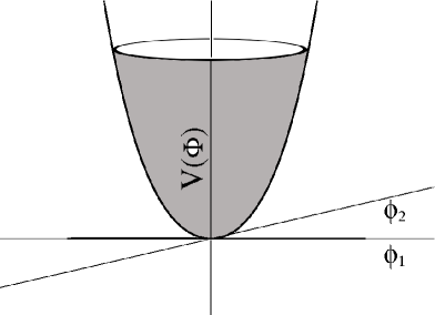
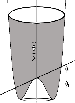
Figure 1.1: The Higgs Potential

In this case the minima will be situated at all $\phi_{1}$ and $\phi_{2}$’s satisfying the condition

$$(\phi_{1}^{2}+\phi_{2}^{2})=v^{2}={-{\rm m}^{2}/\lambda},$$ (1.16)

with the vacuum expectation value (vev) $v=\sqrt{-{\rm m}^{2}/\lambda}$.

The minimum of the potential, now, is not unique and also not at $\Phi=0$, as a result perturbation theory will not be applicable around that point. To pursue it one should shift the field $\Phi(x)$ to

$$\Phi(x)={1\over\sqrt{2}}[v+\eta(x)+i\xi(x)]$$ (1.17)

at one of the minima of the potential. Replacing the $\Phi(x)$ field by eqn.(1.17) in the above Lagrangian of eqn.(1.14) we get

$${\cal L}={1\over 2}\partial_{\mu}\xi\partial^{\mu}\xi+{1\over 2}\partial_{\mu}\eta\partial^{\mu}\eta{-\lambda v^{2}\eta^{2}}-\lambda v\eta^{3}+{\rm other~{}terms}.$$ (1.18)

Due to the above shift of the field $\Phi$, the third term of the modified Lagrangian is, now, the mass term of the field $\eta$ with the mass ${\rm m}_{\eta}=\sqrt{2\lambda v^{2}}=\sqrt{-2{\rm m}^{2}}$. The first term of the modified Lagrangian is the kinetic energy of the $\xi$ field. Note, there is no corresponding mass term for this field which implies that the theory contains a new massless scalar field. If physically there were any such particle we should have detected it. Experimentally, we did not observe any such particle; so does it mean that the spontaneous symmetry breaking mechanism is incorrect? We can easily see from the right figure of Fig. 1.1 that the potential has a flat (circular) direction at the minimum implying the presence of a massless mode. It is a simple example of the Goldstone theorem [3], which states that massless scalars occur whenever a continuous symmetry of a physical system is $``$spontaneously broken” (or, more accurately, is $``$not apparent in the ground state”).

1.4.2 SSB for a local $U(1)$ gauge symmetry

Let us now discuss the spontaneous symmetry breaking mechanism for a local $U(1)$ gauge symmetry which, basically, is known as the Higgs mechanism [4]. What we did in the previous subsection, sec. 1.4.1, is that we had a Lagrangian with a negative (mass)² term and invariant under the global $U(1)$ transformation. Later, we shifted the scalar field to accommodate proper vev. We need a Lagrangian, here, which will be invariant under the local U(1) gauge transformation, eqn.(1.4). The Lagrangian of eqn.(1.14) is not invariant under this local gauge transformation. To make it invariant, as discussed in sec. 1.3, we need a covariant derivative $D_{\mu}$, defined in eqn.(1.10), as

$\partial_{\mu}\rightarrow D_{\mu}\equiv\partial_{\mu}+ieA_{\mu}$

instead of $\partial_{\mu}$ and a gauge field $A_{\mu}$ which simultaneously has to be transformed as

$$A_{\mu}(x)\rightarrow A_{\mu}(x)-{1\over e}\partial_{\mu}\alpha(x).$$ (1.19)

For the ${\rm m}^{2}>0$ scenario, $`$m’ will represent the mass of the scalar field $\Phi$, but we are interested in SSB for which ${\rm m}^{2}<0$. The local $U(1)$ gauge invariant Lagrangian using eqn.(1.12) and eqn.(1.14), thus, is given by

$${\cal L}=-{1\over 4}F_{\mu\nu}F^{\mu\nu}+(\partial_{\mu}-ieA_{\mu})\Phi^{*}(\partial^{\mu}+ieA^{\mu})\Phi-{\rm m}^{2}\Phi^{*}\Phi-\lambda(\Phi^{*}\Phi)^{2}.$$ (1.20)

For SSB, we need to transform the scalar field by eqn.(1.17). The Lagrangian will, thus, be given by

$${\cal L}=-{1\over 4}F_{\mu\nu}F^{\mu\nu}+{1\over 2}\partial_{\mu}\xi\partial^{\mu}\xi+{1\over 2}\partial_{\mu}\eta\partial^{\mu}\eta-\lambda v^{2}\eta^{2}+{1\over 2}e^{2}v^{2}A_{\mu}A^{\mu}-evA_{\mu}\partial^{\mu}\xi+{\rm other~{}terms}.$$ (1.21)

Eqn.(1.21) describes the interaction of a masless boson $\xi$, a massive scalar field $\eta$ of mass $m_{\eta}=\sqrt{2\lambda v^{2}}$ and a massive gauge boson of mass $m_{A}=ev$. So, with the help of the SSB mechanism for a local gauge symmetry we succeeded to generate a mass for the gauge boson. The problem is with the unwanted massless scalar field $\xi$ as we have seen in sec. 1.4.1. Actually, presence of the off-diagonal term $evA_{\mu}\partial^{\mu}\xi$ in the transformed Lagrangian implies that the fields are not in the physical mass basis. We have to reinterpret the particles described by the Lagrangian eqn.(1.21).

For this purpose, it is convenient to use an alternative but equivalent parameterisation of the shifted field $\Phi(x)$. Instead of eqn.(1.17) we write

$$\Phi(x)={1\over\sqrt{2}}[v+h(x)]e^{-i\theta(x)/v}$$ (1.22)

Since the theory is invariant under local $U(1)$ gauge transformations, consider the following transformations, for the set of real fields $h,~{}A_{\mu}$ and $\theta$ as

$$\Phi(x)\rightarrow e^{i\theta(x)/v}\Phi(x)~{}~{}~{}~{}~{}~{}~{}{\rm and}~{}~{}~{}~{}~{}~{}~{}~{}~{}~{}A_{\mu}(x)\rightarrow A_{\mu}(x)-{1\over{ev}}\partial_{\mu}\theta(x).$$ (1.23)

This gauge transformation with the condition that the theory will be independent of the field $\theta(x)$, will help to keep this extra unwanted massless scalar field away. After this transformation, the unwanted field $\theta(x)$ is removed from the theory and using the transformation eqn.(1.23) on eqn.(1.20) we obtain the new transformed Lagrangian as

$${\cal L}=-{1\over 4}F_{\mu\nu}F^{\mu\nu}+{1\over 2}\partial_{\mu}h\partial^{\mu}h-\lambda v^{2}h^{2}+{1\over 2}e^{2}v^{2}A_{\mu}A^{\mu}+{1\over 2}e^{2}vA_{\mu}A^{\mu}h+{\rm other~{}terms}.$$ (1.24)

So as a result of this gauge transformation the unwanted massless scalar field has been absorbed as the longitudinal component of the gauge field $A_{\mu}$. Finally our theory is, now, described by a massive Higgs scalar field $h$ with mass ${\rm m}_{h}=\sqrt{2\lambda v^{2}}$ and the massive gauge boson $A_{\mu}$ with mass ${\rm m}_{A}=ev$.

1.4.3 Higgs mechanism in SM

Let us now come to a more realistic case where, in the SM, the local $SU(2)_{L}\times U(1)_{Y}$ gauge symmetry will spontaneously be broken by the Higgs field, as

$SU(2)_{L}\times U(1)_{Y}\longrightarrow U(1)_{Q}$.

Let us consider the Higgs field, as introduced by Weinberg and defined in eqn.(1.2) and eqn.(1.3), as

$\Phi\equiv\left(\begin{array}[]{c}\phi^{+}\\ \phi^{0}\end{array}\right)\equiv(2,1)\subset(SU(2)_{L}\times U(1)_{Y})$,

where,

$\phi^{+}={1\over{\sqrt{2}}}(\phi_{1}+i\phi_{2})~{}~{}~{}~{}~{}{\rm and}~{}~{}~{}~{}~{}\phi^{0}={1\over{\sqrt{2}}}(\phi_{3}+i\phi_{4}).$

Let us consider the Lagrangian for the field $\Phi$ as

$${\cal L}=\partial_{\mu}\Phi^{\dagger}\partial^{\mu}\Phi-{\rm m}^{2}\Phi^{\dagger}\Phi-\lambda(\Phi^{\dagger}\Phi)^{2}.$$ (1.25)

The Lagrangian, eqn.(1.25), is invariant under the global $SU(2)_{L}\times U(1)_{Y}$ gauge transformation but not under the local $SU(2)_{L}\times U(1)_{Y}$ gauge transformation

$$\Phi(x)\rightarrow e^{i({\vec{\alpha}(x).\vec{\tau}}+\beta(x){Y\over 2})}\Phi(x),$$ (1.26)

where, ${\bf\tau_{a}}$ (a=1,2,3), are the $SU(2)_{L}$ generators and $Y$ the hypercharge as defined in eqn.(1.1).

To make it invariant under the local $SU(2)_{L}\times U(1)_{Y}$ gauge transformation we require, as before, to replace

$$\partial_{\mu}\rightarrow\partial_{\mu}+ig_{2}{\vec{\tau}\over 2}.\vec{W}_{\mu}+ig_{1}{Y\over 2}B_{\mu}.$$ (1.27)

In eqn.(1.27) $g_{1}$ and $g_{2}$ are the $U(1)_{Y}$ and $SU(2)_{L}$ gauge coupling constants respectively. In this case, the gauge field $B_{\mu}$ transforms, as in eqn.(1.11)

$$B_{\mu}\rightarrow B_{\mu}-{1\over{g_{1}}}\partial_{\mu}\beta(x).$$ (1.28)

The $SU(2)_{L}$ gauge boson ${\vec{W}_{\mu}}$ transforms, due to the non-abelian character, as

$$\vec{W}_{\mu}\rightarrow\vec{W}_{\mu}-{1\over{g_{2}}}\partial_{\mu}\vec{\alpha}(x)-\vec{\alpha}\times\vec{W}_{\mu}.$$ (1.29)

This indicates that the rotation of the weak gauge boson, $\vec{W}_{\mu}$, will be affected due to two factors, one, due to the vector nature of the field and another due the variation of the space-time point.

The local $SU(2)_{L}\times U(1)_{Y}$ gauge invariant Lagrangian, thus, can be written as

$${\cal L}=\left[\left(i\partial_{\mu}-g_{2}{\vec{\tau}\over 2}.\vec{W}_{\mu}-{g_{1}\over 2}B_{\mu}\right)\Phi\right]^{\dagger}\left[\left(i\partial^{\mu}-g_{2}{\vec{\tau}\over 2}.{\vec{W}^{\mu}}-{g_{1}\over 2}B^{\mu}\right)\Phi\right]$$

$$-V(\Phi^{\dagger}\Phi)-{1\over 4}{B_{\mu\nu}B^{\mu\nu}}-{1\over 4}{\vec{W}_{\mu\nu}\vec{W}^{\mu\nu}},$$ (1.30)

where $Y=1/2$ is used for the Higgs scalar field.

The scalar potential, $V(\Phi^{\dagger}\Phi)$, is given by

$$V(\Phi^{\dagger}\Phi)={\rm m}^{2}(\Phi^{\dagger}\Phi)+\lambda(\Phi^{\dagger}\Phi)^{2}.$$ (1.31)

The tensors $B_{\mu\nu}$ and $\vec{W}_{\mu\nu}$ are defined as

$$B_{\mu\nu}=\partial_{\mu}B_{\nu}-\partial_{\nu}B_{\mu}$$ (1.32)

and

$$\vec{W}_{\mu\nu}=\partial_{\mu}\vec{W}_{\nu}-\partial_{\nu}\vec{W}_{\mu}-ig_{2}\vec{W}_{\mu}\times\vec{W}_{\nu}.$$ (1.33)

The condition for the spontaneous symmetry breaking is ${\rm m}^{2}<0$ and $\lambda>0$. The minima of the potential are at all those points of $\phi_{i}$s which satisfy the following condition

$$\Phi^{\dagger}\Phi={1\over 2}(\phi_{1}^{2}+\phi_{2}^{2}+\phi_{3}^{2}+\phi_{4}^{2})={v^{2}\over 2}={-{\rm m}^{2}\over{2\lambda}},$$ (1.34)

which implies an infinite number of ground states. The symmetry will spontaneously break once one of it is arbitrarily chosen. Keeping in mind that any unphysical term in the Lagrangian should not be allowed, let us write the scalar field $\Phi$ in terms of four fields $\theta_{1}(x)$, $\theta_{2}(x)$, $\theta_{3}(x)$ and $h(x)$ as:

$$\Phi(x)={1\over{\sqrt{2}}}\left(\begin{array}[]{c}\theta_{2}-i\theta_{1}\\ (v+h)-i\theta_{3}\end{array}\right)\simeq e^{i{\bf\theta_{a}(x)\tau^{a}/}{\it v}}\,\left(\begin{array}[]{c}0\\ \frac{1}{\sqrt{2}}(v+h(x)\,)\end{array}\right)$$ (1.39)

Once we put this transformed field $\Phi$ in the Lagrangian, we will get a massive Higgs field $h$ while the three massless unwanted bosons will disappear from the potential. By an appropriate local gauge transformation - a generalisation of eqn.(1.23) - they may be removed from the theory – effectively absorbed by the $\vec{W}$ bosons as longitudinal components.

1.4.4 Gauge boson and fermion masses

In order to see how the spontaneous breaking of the $SU(2)_{L}\times U(1)_{Y}$ gauge symmetry produces massive $W^{\pm}$ and $Z$ boson while leaving the photon field, $\gamma$, massless let us expand the relevant part of the Lagrangian explicitly:

$$\bigg{|}\bigg{(}-ig_{2}{\vec{\tau}\over 2}.\vec{W}_{\mu}-ig_{1}{1\over 2}B_{\mu}\bigg{)}\Phi\bigg{|}^{2} = {1\over 8}\left|\left(\begin{array}[]{cc}g_{2}W_{\mu}^{3}+g_{1}B_{\mu}&g_{2}(W_{\mu}^{1}-iW^{2}_{\mu})\\ g_{2}(W_{\mu}^{1}+iW^{2}_{\mu})&-g_{2}W_{\mu}^{3}+g_{1}B_{\mu}\end{array}\right)\left(\begin{array}[]{c}0\\ v\end{array}\right)\right|^{2}$$ (1.44)

$$= {1\over 8}g_{2}^{2}v^{2}[(W_{\mu}^{1})^{2}+(W_{\mu}^{2})^{2}]+{1\over 8}v^{2}[g_{2}W_{\mu}^{3}-g_{1}B_{\mu}]^{2}.$$ (1.45)

Let us define the new fields $W^{\pm}_{\mu}$ and $Z_{\mu}$ and it’s orthogonal partner $A_{\mu}$ as

$$W^{\pm}={1\over\sqrt{2}}(W^{1}_{\mu}\mp iW^{2}_{\mu})\ ,\ Z_{\mu}=\frac{g_{2}W^{3}_{\mu}-g_{1}B_{\mu}}{\sqrt{g_{2}^{2}+g_{1}^{2}}}\ ,\ A_{\mu}=\frac{g_{1}W^{3}_{\mu}+g_{2}B_{\mu}}{\sqrt{g_{2}^{2}+g_{1}^{2}}}\$$ (1.46)

to arrive to the form

$${\rm m}_{W}^{2}W^{+}_{\mu}W^{-\mu}+\frac{1}{2}{\rm m}_{Z}^{2}Z_{\mu}Z^{\mu}+\frac{1}{2}{\rm m}_{A}^{2}A_{\mu}A^{\mu}.$$ (1.47)

Finally we have three massive gauge fields $W^{\pm}$ and $Z$ and one massless, the photon field, as needed:

$${\rm m}_{W}=\frac{1}{2}vg_{2}\ ,\ {\rm m}_{Z}=\frac{1}{2}v\sqrt{g^{2}_{2}+g_{1}^{2}}\ ,\ {\rm m}_{A}=0.$$ (1.48)

It is useful to introduce the electroweak mixing angle $\theta_{W}$ defined in terms of the gauge coupling constants $g_{1}$ and $g_{2}$ as

$${\rm sin}\theta_{W}={g_{1}\over{\sqrt{g_{1}^{2}+g_{2}^{2}}}}.$$ (1.49)

It is worthwhile to define a few quantities at this point in terms of the mixing angle $\theta_{W}$. The charged current interactions are

$${1\over 4}{\cal L}_{CC}={G_{F}\over\sqrt{2}}J^{+}_{\mu}{J^{-}}^{\mu},~{}~{}~{}~{}~{}{\rm with}~{}{G_{F}\over\sqrt{2}}={g_{2}^{2}\over{8{\rm m}_{W}^{2}}}$$ (1.50)

and the neutral current interactions are given by

$${1\over 4}{\cal L}_{NC}={G_{F}^{NC}\over\sqrt{2}}J^{0}_{\mu}{J^{\mu}}^{0},~{}~{}~{}~{}~{}{\rm with}~{}G_{F}^{NC}={{g_{1}^{2}+g_{2}^{2}}\over{8{\rm m}_{Z}^{2}}}.$$ (1.51)

An important parameter is the ratio of neutral and charged current interaction strengths, which equals to 1 in the standard model, expressed as

$$\rho={G_{F}^{NC}\over{G_{F}}}={{{\rm m}^{2}_{W}}\over{{\rm m}^{2}_{Z}{\rm cos}^{2}\theta_{W}}}.$$ (1.52)

Let us go back to the problem of gauge invariance for the fermion mass. As the $SU(3)_{C}$ gauge group is chirally blind, without indicating left or right subscripts let us denote the quark as $Q$ and lepton as $L$. Quark is in the triplet $({\bf 3})$ and lepton is singlet $({\bf 1})$ in the $SU(3)_{C}$ group representation. Then the antiquark, $\bar{Q}$, will be in the anti-triplet $({\bf\bar{3}})$ representation. In $SU(3)$ we have,

${\bf 3\otimes\bar{3}\equiv 1\oplus 8}$.

Hence we see that the mass term $\bar{Q}Q$ is invariant under the $SU(3)_{C}$ gauge transformation. For the colour singlet leptons it is an obvious one.

It is quite different for the case of the $SU(2)_{L}$ gauge group. In this case the left and right chiral fermions transform differently as pointed in Table 1.1. A Dirac fermion field can be decomposed as

$$\Psi = \left({{1-\gamma_{5}}\over 2}\right)\Psi+\left({{1+\gamma_{5}}\over 2}\right)\Psi$$ (1.53)

$$= P_{L}\Psi+P_{R}\Psi~{}~{}=~{}~{}\psi_{L}+\psi_{R},$$

where $\psi_{L}$ and $\psi_{R}$ are respectively known as left-chiral and right-chiral fermions.

In the Weyl representation a Dirac fermion field can be written as

$$\Psi=\left(\begin{array}[]{c}\psi_{L}\\ \psi_{R}\end{array}\right).$$ (1.56)

Using eqn.(1.53) the fermion mass term, thus, can be written as

$${\rm m}\bar{\Psi}\Psi\equiv{\rm m}(\bar{\psi}_{L}\psi_{R}+\bar{\psi}_{R}\psi_{L}).$$ (1.57)

Now, from Table 1.1 we see that left-handed fermions are doublet while the right-handed are singlet under the $SU(2)_{L}$ gauge transformation. So neither the term $\bar{\psi}_{L}\psi_{R}$ nor $\bar{\psi}_{R}\psi_{L}$ is invariant, and hence neither is $\bar{\Psi}\Psi$. Thus we see that the fermion mass term ${\rm m}\bar{\Psi}\Psi$ is invariant under the $SU(3)_{C}$ gauge transformation but not under $SU(2)_{L}$.

This problem can be cured with the help of the Higgs scalar multiplet. Using the Higgs doublet we can write an Yukawa interaction term

$$y\bar{\Psi}\Psi\Phi+h.c.$$ (1.58)

where $y$ is the Yukawa coupling. To be more precise, for the first generation lepton sector, we can write,

$$L_{\rm electron}=-y_{e}(\bar{\nu}_{e}~{}~{}\bar{e})_{L}\left(\begin{array}[]{c}\phi^{+}\\ \phi^{0}\end{array}\right)e_{R}+h.c.$$ (1.61)

Once we replace the Higgs field, due to spontaneous symmetry breaking, by

$$\Phi(x)=\left(\begin{array}[]{c}0\\ \frac{1}{\sqrt{2}}(v+h(x)\,)\end{array}\right)$$ (1.64)

we will have a mass term in the Lagrangian as

$$L_{\rm electron}=-{\rm m}_{e}(\bar{e}_{L}e_{R}+\bar{e}_{R}e_{L})~{}~{}~{}{\rm with,}~{}~{}~{}{\rm m}_{e}={y_{e}v\over{\sqrt{2}}}.$$ (1.65)

To generalize for all the matter fields we can write the Yukawa interaction terms, using the notation used in Table 1.1, as

$${\cal L}=-Y^{u}_{ij}\bar{Q}_{L_{i}}{q^{u}_{R_{j}}}\tilde{\Phi}-Y^{d}_{ij}\bar{Q}_{L_{i}}{q^{d}_{R_{j}}}{\Phi}-Y^{l}_{ij}\bar{L}_{L_{i}}{l_{R_{j}}}\Phi+h.c$$ (1.66)

where, $\tilde{\Phi}=-i\sigma_{2}\Phi^{*}$, $Y^{u}$, $Y^{d}$, $Y^{l}$ are the up-quark, down-quark and charged lepton Yuakwa coupling constant matrices respectively. One point to be noted is that the particle content, listed in the Table 1.1, in the SM does not contain any right-handed neutrino. It was conspired just to explain the then accepted zero mass of the neutrino. Once, the Higgs field gets a $vev$, $v$, then the Lagrangian takes the form $\overline{f_{L}}m_{f}f_{R}$ with the mass matrices

$${({\rm m}_{u})}_{ij}=Y^{u}_{ij}v,{({\rm m}_{d})}_{ij}=Y^{d}_{ij}v,{({\rm m}_{l})}_{ij}=Y^{l}_{ij}v,$$ (1.67)

where, $f=(u,c,t)^{T}~{}{\rm or}~{}(d,s,b)^{T}~{}{\rm or}~{}(e,\mu,\tau)^{T}$ represent the three generations of fermion fields. These mass matrices are in the flavour basis, not the mass basis.

1.5 Shortcomings of the standard model

Some unattractive features of the standard model have been noted in sec. 1.1. Besides the non-zero neutrino mass, there are several conceptual shortcomings of the standard model. The standard model contains 19 parameters - three gauge couplings $g_{1}$, $g_{2}$, $g_{3}$, six quarks and three charged-leptons masses, one CP-violating phase, three CKM mixing angles, the quadratic and quartic coupling constants for the Higgs scalar potential and strong CP parameter. The standard model does not say anything about the fourth force, namely the gravitational interaction. At the scale of Planck mass, $M_{P}$, we need a theory of quantum gravitation which will also describe the dynamics of particles governed by the gravitational interaction in addition with other forces. Although, to reduce the large number of parameters one can extend the theory of unification, but the point one may ask is can it predict different observables like mixing angles, fermion masses etc properly? What is the origin of three generations of fermions?

In order to remove these shortcomings, physicists have come up with different new options like Grand Unified Theory (GUT), Supersymmetry, Extra Dimensions etc. to extend the standard model. A brief introduction to these are given below.

1.6 Grand unified theory

A general aesthetic of physics is that the more symmetrical a theory is, the more $``$beautiful” and $``$elegant” it is. In this view, the Standard Model gauge group, which is the direct product of three groups, is not a truly satisfactory one. In analogy with the 19th-century unification of electricity with magnetism into electromagnetism, and especially the success of the electroweak theory, which utilizes the idea of spontaneous symmetry breaking as discussed in previous sections, to unify electromagnetism with the weak interaction, it is natural to attempt to unify all three groups in a similar manner. Three independent gauge coupling constants and a huge number of Yukawa coupling coefficients require far too many parameters, and it would be elegant if these coupling constants could be explained by a theory with fewer parameters. A gauge theory based on a simple group has only one gauge coupling constant, and since the fermions are now grouped together in larger representations, there are fewer Yukawa coupling coefficients as well. In order to get unification [5] of all three interactions we need a bigger group which will contain the standard model gauge group $SU(3)_{C}\times SU(2)_{L}\times U(1)_{Y}$ and, in addition, this gauge group has to break down to the standard model gauge group at some higher scale in such a way that it will predict different mass and mixing angles at the low energy scale.

1.6.1 $SU(5)$ GUT model

The first attempts of grand unification were made by Pati and Salam [6] to unify quarks and leptons within $SU(2)_{L}\times SU(2)_{R}\times SU(4)_{C}$, known as the Pati-Salam gauge group $({\cal G}_{PS})$. In this scenario lepton is treated as the fourth component of the colour quantum number of the $SU(4)_{C}$ gauge group. Another approach independently proposed by Georgi and Glashow in 1973 [7] considers $SU(5)$, which is of rank 4 (same as the SM gauge group), as the unified group. It has a few advantages; like, it gives a beautiful way of unifying all the three standard model gauge couplings. In this $SU(5)$ GUT model there is a unique way to accommodate all the fifteen quarks and leptons in the $\bar{5}$ and $10$ representations. The break up of these two multiplets of the $SU(5)$ group in terms of the SM gauge group $SU(3)_{C}\times SU(2)_{L}\times U(1)_{Y}$ are:

$$5\equiv(3,1,-{1\over 3})\oplus(1,2,{1\over 2})~{}~{}~{}{\rm and}~{}~{}~{}10\equiv(1,1,1)\oplus(\bar{3},1,-{2\over 3})\oplus(3,2,{1\over 6}).$$ (1.68)

The right-handed down quark $d\equiv(d^{r},d^{g},d^{b})$ and right-handed $(e^{+},\tilde{\nu_{e}})$ doublet can preferably be put into the $\bar{5}$ representation respectively. On the other hand the singlet charged left-handed anti-lepton $e^{+}$, the left-handed $u,d$ quark doublet and left-handed anti-u quark singlet $u^{c}$ will be in $10$, the antisymmetric part of the product of two 5 plets.

Similarly, $24(=5^{2}-1)$ gauge bosons associated with the $SU(5)$ gauge group can be decomposed as follows:

$$24\equiv(8,1,0)+(1,3,0)+(1,1,0)+(3,2,-{5\over 6})+(\bar{3},2,{5\over 6})$$ (1.69)

which are the gluons, electro-weak gauge bosons and the new heavy X,Y gauge bosons. These new gauge bosons, X and Y, mediate the proton decay. One can have, for example, for the decay mode,

$$M(p\rightarrow e^{+}\pi^{0})\sim{g^{2}\over{{\rm m}^{2}_{X}}},$$ (1.70)

where g is the GUT gauge coupling constant. Hence, the proton lifetime is

$$\tau_{p}\sim{{{\rm m}^{4}_{X}}\over{g^{4}{{\rm m}_{p}^{5}}}}.$$ (1.71)

Non-observation of proton decay puts a lower limit on these heavy gauge boson masses

$${\rm m}_{X,Y}~{}>~{}10^{15}~{}{\rm GeV}$$ (1.72)

We have the normalisation of the generators of the GUT gauge group as

$${\rm Tr}(t^{a}t^{b})=N\delta^{ab}$$ (1.73)

where, N is the normalisation constant. Invariance under the gauge group G means all observed gauge couplings are the same as that of the unified gauge group. Unlike the $SU(2)_{L}$ and $SU(3)_{C}$ couplings, eqn. (1.73) does not fix the scale of the $U(1)_{Y}$ coupling constant. It would not change the physics if we divide it by a constant factor $c$ and simultaneously multiply the hypercharge $Y$ by the same factor.

As stated above, considering ${{\tau^{a}}\over{2}}$ as the $SU(2)$ generators we choose,

$${\rm Tr}\big{(}{\tau^{a}\over 2}{\tau^{b}\over 2}\big{)}={1\over 2}\delta^{ab}.$$ (1.74)

So, let us assume that the $Y=c({y\over 2})$ is the generator of the unified gauge group, in addition with the unchanged $SU(2)_{L}$ and $SU(3)_{C}$ generators. Now, in the unified scenario all the generators have common normalisation factor as a result we have,

$${\rm Tr}(c^{2}(y/2)^{2})={\rm Tr}(T_{3})^{2}$$ (1.75)

with $T_{3}$, the third $SU(2)_{L}$ generator. The trace is over all particle states in the representation. In the SM framework for one generation these are u, d, $\nu_{e}$ and $e^{-}$. Thus for the above relation we have,

$$3(\frac{1}{4}+\frac{1}{4})+\frac{1}{4}+\frac{1}{4}=c^{2}\big{(}3({1\over 6})^{2}+3({1\over 6})^{2}+3({2\over 3})^{2}+3(-{1\over 3})^{2}+(-{1\over 2})^{2}+(-1)^{2}+(-{1\over 2})^{2}\big{)}.$$ (1.76)

This implies,

$$c=\sqrt{3\over 5},$$ (1.77)

and, hence the properly normalized generator is

$$Y=\sqrt{3\over 5}{y\over 2}.$$ (1.78)

Thus, for the standard model scenario, we have

$$g_{SU(5)}=g_{1}\sqrt{5\over 3}~{}~{}~{}~{}{\rm and}~{}~{}~{}~{}~{}g_{SU(5)}=g_{2},$$ (1.79)

and (eqn.(1.49)) leads to ${\rm tan\theta_{W}}=\sqrt{3\over 5}$, hence, ${\rm sin^{2}\theta_{W}}={3\over 8}$.

Generally, the $SU(5)$ symmetry is broken down to the low energy $SU(3)_{C}\times U(1)_{Q}$ by two Higgs scalars $\Phi_{24}$ and $H_{5}$ which are in the adjoint 24 and 5 of $SU(5)$. The breakdown of these two Higgs multiplets in the $SU(3)_{C}\times SU(2)_{L}\times U(1)_{Y}$ representation are given in eqns. (1.69) and (1.68) respectively.

When the neutral component $(1,1,0)$ of the the $\Phi_{24}$ gets a vev at the GUT scale, $SU(5)$ breaks to the SM gauge group while getting a nonzero vev for $H_{5}$ at the electro-weak scale breaks the SM down to $SU(3)_{C}\times U(1)_{Q}$.

The stepwise breakdown of the gauge symmetry in this case, thus, is

$${SU(5)}~{}{\Phi_{24}\over(M_{U})}{\rightarrow}~{}{SU(3)_{C}\times SU(2)_{L}\times U(1)_{Y}}~{}{H_{5}\over(M_{Z})}{\rightarrow}~{}{SU(3)_{C}\times U(1)_{Q}}.$$ (1.80)

Gauge hierarchy problem

A major difficulty of the standard model is the gauge hierarchy problem [8]. In order to realise this hierarchy between $M_{U}$ and $M_{Z}$ and hence the problem of naturalness let us calculate the quadratic divergence for the Higgs mass due to standard model fermions.

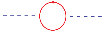
Figure 1.2: One loop fermionic correction to the Higgs mass

The one loop correction to the Higgs mass ${\rm m}_{H}$ is obtained by calculating the two point function:

$$\Pi^{f}_{hh} = (-1)\int{d^{4}k\over(2\pi)^{4}}{\rm Tr}\left\{({-i\lambda_{f}\over\sqrt{2}}){i\over{\not k-{\rm m}_{f}}}({-i\lambda_{f}\over\sqrt{2}}){i\over{\not k-{\rm m}_{f}}}\right\},$$ (1.81)

where $\lambda_{f}$ is the fermion-scalar-fermion coupling constant. The loop momentum $k$ can take any value from zero to infinity. This leads to a correction which is infinite and makes the theory ill-defined. So, we assume that our theory is valid upto a cut-off scale $\Lambda$. The above integration, thus, becomes

$$\Pi^{f}_{hh} = -2\lambda_{f}^{2}\int_{0}^{\Lambda}{d^{4}k\over{(2\pi)^{4}}}\left[{1\over{k^{2}-{\rm m}_{f}^{2}}}+{2{\rm m}_{f}^{2}\over{(k^{2}-{\rm m}_{f}^{2})^{2}}}\right]$$ (1.82)

$$= {-{\lambda_{f}^{2}\over{8\pi^{2}}}\Lambda^{2}}+...$$

Thus the corrected Higgs $($mass${\rm)}^{2}$ is

$${\rm m}_{H}^{2}={\rm m}_{H_{0}}^{2}+\delta{\rm m}_{H}^{2}$$ (1.83)

where the correction $\delta{\rm m}_{H}^{2}$ is proportional to the $\Pi^{f}_{hh}$. In GUT we have a new scale at $10^{16}~{}~{}{\rm GeV}$. If there is no new physics before this scale then $\Lambda\sim 10^{16}~{}~{}{\rm GeV}$ and to have a Higgs mass of ${\cal O}(100~{}{\rm GeV})$ a fine-tuning of the co-efficient $\lambda_{f}$ to 1 part in $10^{26}$ is needed.

1.6.2 $SO(10)$ GUT model

$SO(10)$ is a possible useful GUT gauge group for the unification of the SM [9]. It is a group of rank 5, unlike the SM gauge group which is of rank 4. As the rank is the maximum number of diagonal generators of the group, so the extra diagonal generator of this unified gauge group will define another quantum number, which can be identified as $(B-L)$ for the left-right symmetric version of this theory. Due to the presence of an extra diagonal generator, $SO(10)$ can be broken to the standard model in various ways.

One good feature for the group is that in a single multiplet $16$ it can accommodate all the standard model fermions in addition with a standard model gauge singlet right-handed neutrino, needed to explain the tiny neutrino mass. This group can support left-right symmetry, represented by the gauge group $SU(3)_{C}\times SU(2)_{L}\times SU(2)_{R}\times U(1)_{(B-L)}\equiv{\cal G}_{LR}$. We consider this class of $SO(10)$ models below.

There are two broad classes of minimal $SO(10)$ models: those with only doublet Higgs scalars (Model I) and the conventional left-right symmetric model including triplet Higgs scalars (Model II). In both versions, a bi-doublet Higgs scalar $\Phi~{}\equiv(1,2,2,0)$ under ${\cal G}_{LR}$, gives mass to the charged fermions and also a Dirac mass to the neutrinos. In an $SO(10)$ GUT, this bi-doublet $\Phi$ belongs to the representation ${\bf 10,120}$ or ${\bf 126}$. Usually a ${\bf 10}$ representation is chosen. However, for correct fermion mass relations [10], a ${\bf\overline{126}}$ representation containing the field $\Phi^{\prime}\equiv\{15,2,2\}$ under the group $SU(4)_{C}\times SU(2)_{L}\times SU(2)_{R}\equiv{\cal G}_{PS}$ is often also included.

The main differences between Models I and II lie in the Higgs sector and the generation of neutrino masses. Lepton number violation in these models arises from the Higgs scalars that break the $B-L$ symmetry and hence the left-right symmetry. In Model I, the left-right symmetric group ${\cal G}_{LR}$ is broken by an $SU(2)_{R}$ doublet Higgs scalar $\chi_{R}\equiv(1,1,2,-1)$ when its neutral component acquires a $vev$ $\langle\chi^{\circ}_{R}\rangle\sim v_{R}$. Left-right parity implies the presence of an $SU(2)_{L}$ doublet Higgs scalar $\chi_{L}\equiv(1,2,1,-1)$. The $vev$ of the neutral component of this field, $\langle\chi^{\circ}_{L}\rangle\sim v_{L}$, in addition to $\langle\Phi\rangle$, breaks the electroweak symmetry.

In Model II, an $SU(2)_{R}$ triplet Higgs scalar $\bar{\Delta}_{R}\equiv(1,1,3,2)$ breaks the left-right symmetric group ${\cal G}_{LR}$. When the neutral component acquires a $vev$, $\langle{\bar{\Delta}}^{\circ}_{R}\rangle\sim v_{R}$, it gives Majorana masses to the right-handed neutrinos breaking lepton number by two units. When the bi-doublet Higgs scalar $\Phi$ breaks the electroweak symmetry, this leads to the small see-saw neutrino mass [11]. Due to left-right parity, there is also an $SU(2)_{L}$ triplet Higgs scalar $\bar{\Delta}_{L}\equiv(1,3,1,2)$. Although these scalars have a mass at the parity breaking scale $M_{R}$, the $vev$ of the neutral component of this field is extremely tiny and can give small Majorana masses to the left-handed neutrinos leading to a new type of see-saw mechanism.

Models I and II have the same symmetry breaking chain:

$$SO(10) \stackrel{{\scriptstyle 210~{}(M_{U})}}{{\longrightarrow}} SU(3)_{C}\times SU(2)_{L}\times SU(2)_{R}\times U(1)_{B-L}$$

$$\stackrel{{\scriptstyle 16~{}{\rm or}~{}126~{}(M_{R})}}{{\longrightarrow}} SU(3)_{C}\times SU(2)_{L}\times U(1)_{Y}$$

$$\stackrel{{\scriptstyle 10~{}(M_{Z})}}{{\longrightarrow}} SU(3)_{C}\times U(1)_{Q}$$

At the GUT scale, the symmetry is broken by the vacuum expectation value of a ${\bf 210}$-dimensional representation of $SO(10)$. The ${\bf 210}$ has a singlet under the subgroup ${\cal G}_{PS}$, i.e., $\{1,1,1\}$, which is odd under parity. When this field acquires a $vev$, $SO(10)$ is broken to ${\cal G}_{PS}$ and D-parity is also spontaneously broken (i.e., $g_{2L}\neq g_{2R}$). To keep D-parity intact at this level we have to look elsewhere. The $SO(10)$ 210 also contains a {15,1,1} under ${\cal G}_{PS}$ which is D-parity even. This is the field to which the $vev$ must be ascribed to get the desired symmetry breaking to ${\cal G}_{LR}$ while keeping D-parity intact.

The left-right symmetry, ${\cal G}_{LR}$, is broken by the $vev$ of the fields $F+\bar{F}$, where $F$ is a ${\bf{16}(\equiv\bf{\Gamma})}$-dimensional representation for Model I and a ${\bf 126}$-dimensional representation for Model II. Finally, the electroweak symmetry breaking takes place by the $vev$ of a 10-plet of $SO(10)$. In the minimal models under consideration, there are no other Higgs representations.

The breakdown [12] of the 16 multiplet of $SO(10)$ under the $SU(4)_{C}\times SU(2)_{L}\times SU(2)_{R}$ is

$$16\equiv(4,2,1)\oplus(\bar{4},1,2).$$ (1.84)

This 16-multiplet, thus, in addition with the left-handed particles also contains the left-handed anti-particles (equivalently the right-handed particles).

A 16-dimensional multiplet can be written as

$$\Psi=\left(\begin{array}[]{c}\psi_{0}\\ \psi_{j}\\ \psi_{jk}\end{array}\right)$$ (1.88)

where, in the language of $SU(5)$ representations

$$\Psi(16)\equiv\psi_{0}(1)\oplus\psi_{j}(\bar{5})\oplus\psi_{ij}(10)$$ (1.89)

with,

$$\psi_{0}=N^{c},~{}~{}\psi_{j}\equiv L+d^{c}\equiv\left(\begin{array}[]{c}d^{c}_{1}\\ d^{c}_{2}\\ d^{c}_{3}\\ e^{-}\\ {\nu}_{e}\end{array}\right),~{}~{}\psi_{ij}\equiv(Q+U^{c}+E^{c})\equiv\left(\begin{array}[]{ccccc}0&u^{c}_{3}&-u^{c}_{2}&u_{1}&d_{1}\\ &0&u^{c}_{1}&u_{2}&d_{2}\\ &&0&u_{3}&d_{3}\\ &&&0&e^{+}\end{array}\right).$$ (1.99)

Let us consider the following symmetry breaking chain

$$SO(10) \stackrel{{\scriptstyle 210~{}(M_{U})}}{{\longrightarrow}} SU(3)_{C}\times SU(2)_{L}\times SU(2)_{R}\times U(1)_{B-L}$$

$$\stackrel{{\scriptstyle 16~{}{\rm or}~{}126~{}(M_{R})}}{{\longrightarrow}} SU(3)_{C}\times SU(2)_{L}\times U(1)_{Y}$$

$$\stackrel{{\scriptstyle 10~{}(M_{Z})}}{{\longrightarrow}} SU(3)_{C}\times U(1)_{Q}$$

An obvious question comes in our mind is what is the normalisation factor for the $B-L$ quantum number, c.f. the case of the hypercharge quantum number in sec. 1.6.1. Let us define different quantum numbers for all the members of a 16-dimensional multiplet in the $SU(2)_{L}\times SU(2)_{R}\times U(1)_{B-L}\times SU(3)_{C}$ group notation as:

$$Q_{L}\equiv\left(\begin{array}[]{c}u\\ d\end{array}\right)_{L}\equiv(2,1,{1\over 3},3)\subset{\bf 16},~{}~{}~{}~{}~{}\psi_{L}\equiv\left(\begin{array}[]{c}\nu\\ e\end{array}\right)_{L}\equiv(2,1,-1,1)\subset{\bf 16},$$ (1.104)

$$Q_{R}\equiv\left(\begin{array}[]{c}u\\ d\end{array}\right)_{R}\equiv(1,2,{1\over 3},3)\subset{\bf 16},~{}~{}~{}~{}~{}\psi_{R}\equiv\left(\begin{array}[]{c}\nu\\ e\end{array}\right)_{R}\equiv(1,2,-1,1)\subset{\bf 16}.$$ (1.109)

For these particles we have,

$Tr\left(k^{2}({B-L\over 2})^{2}\right)=k^{2}\left(3({1\over 6})^{2}+3({1\over 6})^{2}+3({1\over 6})^{2}+3({1\over 6})^{2}+(-{1\over 2})^{2}+(-{1\over 2})^{2}+(-{1\over 2})^{2}+(-{1\over 2})^{2}\right)$

$$=k^{2}{4\over 3}\hskip 295.90848pt$$ (1.110)

where, the factor 3 arises due to colour while $`k$’ is the normalisation factor to be determined. In comparison with the Trace of the $SU(2)$ generator, which is

$$Tr\left({I_{3L}^{2}\over 2}\right)=3(\frac{1}{4}+\frac{1}{4})+\frac{1}{4}+\frac{1}{4}=2$$ (1.111)

we have ${4\over 3}k^{2}=2$ i.e. $k=\sqrt{3\over 2}$.

1.6.3 Renormalisation group equations

The renormalisation group, in quantum field theory, tells us how different couplings evolve with energy. But before discussing the renormalisation group equations (RGE) an obvious question is: what is renormalisation [2]? In QFT, Green function is a most important thing to be calculated. In perturbative QFT these quantities are divergent. The systematic way to remove these divergences is known as renormalisation. There are different ways to cancel these infinities. In order to renormalise the theory we need a reference point which is also arbitrary. Different choices of this reference point lead to different sets of parameters for the theory, but physics should not depend on the arbitrary choice of the reference point and be invariant. This invariance leads to the renormalisation group. In quantum field theory it is a useful method to examine the behaviour of physics at a different scale knowing the same at some other scale. Thus, measuring the observables in a low energy experiment one can compare with the values predicted from a theory at a higher scale, e.g at the GUT scale and certify about the correctness of the theory. In the standard model, variations of the gauge coupling constants with energy are given by the following renormalisation group equations (RGEs)

$$16{\pi}^{2}E{dg_{i}\over dE}=b_{i}g_{i}^{3}=\beta_{SM}(g_{i})$$ (1.112)

where $i$ stands for $U(1)_{Y},~{}SU(2)_{L}~{}{\rm and}~{}SU(3)_{C}$ and the right-hand-side is known as the $\beta$-function of the corresponding coupling. One can write this equation as

$${d\over{dlnE}}{{\alpha}_{i}}^{-1}(E)=-{b_{i}\over 2\pi}.$$ (1.113)

where, $\alpha_{i}={{g^{2}_{i}}\over{4\pi}}$.

Using the measured values of these coupling constants at the scale $M_{Z}$ as the initial values one can solve these equations as,

$${\alpha}_{i}^{-1}(E)={\alpha}_{i}^{-1}(M_{Z})-{b_{i}\over 2\pi}{\rm ln}{E\over M_{Z}}.$$ (1.114)

In the above equations the co-efficients, $b_{i}$, can be calculated for any $SU(N)$ group as

$$b_{i}=-{11\over 3}C_{2}(G)+{2\over 3}n_{f}C_{2}(R)+{1\over 3}n_{s}C_{2}(R)$$ (1.115)

where $C_{2}(R)$ is the quadratic Casimir operator for the representation R while $C_{2}(G)$ is that for the adjoint representation. These Casimir operators are discussed below. In the above equation $n_{f}$ is the number of chiral fermions and $n_{s}$ is the number of complex scalars contributing to the $\beta$-function.

The generators of a gauge group obey the following rules

$$Tr[t_{R}^{a}t_{R}^{b}]=C(R)\delta^{ab},$$ (1.116)

and

$$\sum_{a}t_{R}^{a}t_{R}^{a}=C_{2}(R).\bf{1}$$ (1.117)

where, the proportionality constant $C_{2}(R)$ is the quadratic Casimir operator for the particular representation. One can easily show that the quadratic Casimir operator is related with the factor $C(R)$ via

$$C_{2}(R)d(R)=C(R)r$$ (1.118)

where, $r$ is the number of generators $(=N^{2}-1)$ of the $SU(N)$ gauge group, equivalent to the dimension of the adjoint representation, and $d(R)$ is the dimension of the representation R.

According to the convention used in eqn.(1.74), the $SU(2)$ generators follow the relation

$$Tr[{\tau^{a}\over 2}{\tau^{b}\over 2}]={1\over 2}\delta^{ab}.$$ (1.119)

As stated earlier the bigger GUT $SU(N)$ group will be chosen in such a way that it will contain the $SU(2)$ as a subgroup. The generators of the $SU(N)$ will also follow the same normalisation condition – eqn.(1.119) – and, thus, we have $C(R)={1\over 2}$ in the fundamental representation. Immediately eqn.(1.118) implies that for $R=N$, i.e for the fundamental representation the quadratic Casimir operator is $C_{2}(N)={{N^{2}-1}\over{2N}}$. For the adjoint representation $C_{2}(G)=N$. For the $U(1)$ gauge group these values will be $C_{2}(G)=0$ and $C_{2}(R)=C(R)=(Y/2)^{2}$.

Figure 1.3: Evolution of the gauge couplings in the standard model

So, for the standard model, considering the contribution of all the particles listed in Table 1.1 one has for the three different co-efficients for the gauge groups $U(1)_{Y}$, $SU(2)_{L}$ and $SU(3)_{C}$

$$\left(\begin{array}[]{c}b_{Y}\\ b_{2L}\\ b_{3C}\end{array}\right)=\left(\begin{array}[]{c}{41\over 10}\\ -{19\over 6}\\ -7\end{array}\right).$$ (1.126)

where, the GUT normalisation factor ${3\over 5}$ is already multiplied to calculate the co-efficient for the $U(1)_{Y}$ gauge group. Using these values of $`b$’ one can find the evolution of the gauge couplings with energy from eqn(1.114) as depicted in Fig. 1.3 upto one loop contribution only.

It shows that all three standard model gauge couplings are trying to unify at some higher scale $\sim 10^{15}$ GeV, comparable to the predicted value of $M_{G}$ from the proton decay limits. Although in this case they are not unifying exactly, they do so in the supersymmetric scenario.

1.7 Supersymmetry

Supersymmetry is a space-time symmetry which relates the bosonic degrees of freedom to the fermionic degrees of freedom [14, 15, 16]. The beautiful idea of supersymmetry helps to solve the gauge hierarchy problem (1.6.1). The one loop radiative correction for the Higgs mass due to scalar particles in the loop is

$$\delta{\rm m}_{H}^{2}={\lambda_{S}\over{16\pi^{2}}}[\Lambda^{2}-2{\rm m}_{S}^{2}{\rm ln}{\Lambda\over{M_{S}}}-...],$$ (1.127)

where $\lambda_{S}$ is the corresponding coupling for the term in the Lagrangian, viz. $-\lambda_{S}H^{2}S^{2}$. The same correction for a fermion-antifermion pair in loop takes the form

$$\delta{\rm m}_{H}^{2}={|\lambda_{f}|^{2}\over{8\pi^{2}}}\left[-\Lambda^{2}+3{\rm m}_{f}^{2}{\rm ln}(\Lambda/{\rm m}_{f})+...\right],$$ (1.128)

with $\lambda_{f}$ the coefficient of the term $-\lambda_{f}Hf\bar{f}$ in the Lagrangian.

So, we see that a conspiracy between the bosonic and fermionic degrees of freedom can solve the hierarchy problem. If we postulate that corresponding to each chiral fermion there should be a complex scalar and vice versa with the condition

$$\lambda_{S}=|\lambda_{f}|^{2},$$ (1.129)

which follows in a supersymmetric theory, then the quadratic correction can be erased.

In a supersymmetric transformation a boson changes to a fermion and vice versa. Thus, if $Q$ is the generator of this transformation then

$$Q|boson\rangle\equiv|fermion\rangle,~{}~{}~{}{\rm and}~{}~{}Q|fermion\rangle\equiv|boson\rangle.$$ (1.130)

Hence, the generator Q has to be fermionic in nature with spin angular momentum $1/2$ which is why supersymmetry is a space-time transformation.

The irreducible representation in which a particle and its superpartner will be accommodated is known as the supermultiplet. The number of bosonic and fermionic degrees of freedom are equal in each supermultiplet. There are different types of supermultiplets– the simplest one is the chiral or matter supermultiplet. It contains a chiral Weyl spinor and a complex scalar field, both of them are of two degrees of freedom. The gauge or vector supermultiplet is the one in which a massless spin-1 vector gauge boson (degrees of freedom 2) is kept with it’s fermionic superpartner, a massless spin-1/2 Majorana fermion, known as the gaugino. The Minimal Supersymmetric Standard Model (MSSM), thus, contains the standard model particles, Table 1.1, and their corresponding superpartners. The particles in the MSSM are listed in Table 1.2.

Names		spin 0	spin 1/2	$SU(3)_{C},\,SU(2)_{L},\,U(1)_{Y}$
squarks, quarks	$Q$	$({\widetilde{u}}_{L}\>\>\>{\widetilde{d}}_{L})$	$(u_{L}\>\>\>d_{L})$	$(\>{3},\>{2}\>,\>{1\over 6})$
	$\overline{u}$	${\widetilde{u}}^{*}_{R}$	$u^{\dagger}_{R}$	$(\>{\overline{3}},\>{1},\>-{2\over 3})$
	$\overline{d}$	${\widetilde{d}}^{*}_{R}$	$d^{\dagger}_{R}$	$(\>{\overline{3}},\>{1},\>{1\over 3})$
sleptons, leptons	$L$	$({\widetilde{\nu}}\>\>{\widetilde{e}}_{L})$	$(\nu\>\>\>e_{L})$	$(\>{1},\>{2}\>,\>-{1\over 2})$
	$\overline{e}$	${\widetilde{e}}^{*}_{R}$	$e^{\dagger}_{R}$	$(\>{1},\>{1},\>1)$
Higgs, higgsinos	$H_{1}$	$(H_{1}^{+}\>\>\>H_{1}^{0})$	$(\widetilde{H}_{1}^{+}\>\>\>\widetilde{H}_{1}^{0})$	$(\>{1},\>{2}\>,\>+{1\over 2})$
	$H_{2}$	$(H_{2}^{0}\>\>\>H_{2}^{-})$	$(\widetilde{H}_{2}^{0}\>\>\>\widetilde{H}_{2}^{-})$	$(\>{1},\>{2}\>,\>-{1\over 2})$
		spin 1/2	spin 1
gluino, gluon		$\widetilde{g}$	$g$	$(8,1,0)$
winos, W-bosons		$\widetilde{W}^{\pm}$, $\widetilde{W}^{0}$	${W^{\pm}}$, ${W^{0}}$	$(1,3,0)$
bino, B-boson		$\widetilde{B}^{0}$	${B^{0}}$	$(1,1,0)$

Table 1.2: Supersymmetric partners with the Standard Model members

Note that in Table 1.2 MSSM requires two Higgs doublets for the following good reasons. Firstly, to keep the theory free from triangle gauge anomalies we need two Higgs scalar doublet. Since, the condition for a theory to be free from gauge anomalies is

$$\sum_{\rm Weyl~{}fermions}{\rm Tr}\left(({y\over 2})^{3}\right)=\sum_{\rm Weyl~{}fermions}{\rm Tr}\left(T^{2}_{3}{y\over 2}\right)=0.$$ (1.131)

The standard model itself was anomaly free, but supersymmetric extension of the SM brings one Weyl spinor, namely the Higgsino $\widetilde{H_{1}}$ with hypercharge $+{1\over 2}$. This will generate anomalies. So if we add a new Higgs multiplet $(H_{2},~{}\widetilde{H_{2}})$ with hypercharge opposite to that of the $H_{1}$ multiplet, then the anomaly will be cancelled again.

Secondly, to make the up-type quarks massive we used $\Phi^{*}$ in sec. 1.4.4. Analyticity of the superpotential forces a field of definite chirality only and hence the use of the complex conjugate of a field is disallowed. The two complex scalar doublets are

$${H_{1}}=\left(\begin{array}[]{c}{H_{1}}^{0}\\ {H_{1}}^{-}\end{array}\right),~{}~{}~{}~{}~{}{H_{2}}=\left(\begin{array}[]{c}{H_{2}}^{+}\\ {H_{2}}^{0}\end{array}\right),$$ (1.136)

After spontaneous symmetry breaking the minimum of $V_{0}$ involves the following two vevs: $\langle H_{1}^{0}\rangle=v_{1}$ and $\langle H_{2}^{0}\rangle=v_{2}$. The combination $v=\sqrt{v_{1}^{2}+v_{2}^{2}}=(\sqrt{2}G_{F})^{-1/2}\simeq 246$ GeV sets the Fermi scale. These two different vevs will contribute to the up- and down-type quark masses respectively. The ratio of these two vevs,

$$\tan\beta=\frac{v_{2}}{v_{1}}$$ (1.137)

is a very useful parameter for the discussion of the supersymmetric phenomenology.

In a supermultiplet both the particle and its superpartner are included, so for exact supersymmetry both the members should have the same mass. If the superpartners were of same masses, they would have been already detected in experiments. So far, none of the superpartners is observed. So, supersymmetry is a broken symmetry. On the other hand, Yuakwa-type coupling constants for the particles and corresponding antiparticles are already fixed by eqn.(1.129) due to supersymmetry. The supersymmetry, thus, will be broken softly; that means the coefficients of supersymmetry breaking couplings should be of mass dimension less than four and positive in order to cure the gauge hierarchy problem between the electroweak scale and a higher scale like, GUT or Planck scale. There are various models to predict the mass spectra for the MSSM scenario. In general, it is assumed that the origin of supersymmetry breaking is at some higher scale and that all the superpartner masses will be around the scale $M_{S}\sim{\rm TeV}$, known as the SUSY scale.

1.7.1 Gauge unification in SUSY

The one-loop renormalisation group equations for the MSSM case is

$$16{\pi}^{2}E{dg_{i}\over dE}=b_{i}g_{i}^{3}+\Theta(E-M_{S})(\widetilde{b_{i}}-b_{i})g_{i}^{3}={\beta}_{MSSM}(g_{i}),$$ (1.138)

where, $\Theta$ is a step function, used due to the fact that the standard model is valid upto scale $M_{S}$ after which supersymmetry will come into play. The standard model b-coefficients $`b_{i}$’ are given by eqn.(1.115) while the MSSM b-coefficients are:

$$\left(\begin{array}[]{c}{\widetilde{b}_{Y}}\\ {\widetilde{b}_{2L}}\\ {\widetilde{b}_{3C}}\end{array}\right)=\left(\begin{array}[]{c}{33\over 5}\\ 1\\ -3\end{array}\right).$$ (1.145)

Figure 1.4: Evolution of the gauge couplings in the supersymmetric scenario

These are the contributions due to the whole supermultiplet i.e both from the SM particles and the corresponding superpartners. As a result not to overcount the contributions from the SM particles, the standard model b-coefficients $`b_{i}$’ are subtracted out from the second term in eqn.(1.138). The evolution of the gauge couplings, thus, is given by

$$\alpha_{i}^{-1}(E)=\alpha_{i}^{-1}(M_{Z})-{b_{i}\over 2\pi}ln{M_{S}\over M_{Z}}-\Theta(E-M_{S})\left({{\widetilde{b_{i}}-b_{i}}\over{2\pi}}\right){\rm ln}{E\over M_{S}}.$$ (1.146)

The evolution of the gauge couplings $\alpha_{i}(={g^{2}_{i}\over 2\pi})$ is depicted in Fig. 1.4. We have already seen that supersymmetry can solve the gauge hierarchy problem, but in addition Fig. 1.4 shows that it’s particle content is such that it also gives a very good unification of the standard model gauge couplings. Also, the unification, like in the SM case, is at such a high scale then it will not conflict with the proton life time predicted in sec. 1.6.1.

1.8 Extra dimensions

In the SM we have seen that the hierarchy problem is arising due to the huge ratio of the Planck scale, ${M_{Pl}}$, or the GUT scale, ${M_{G}}$, to the electroweak scale. As discussed in the previous section, supersymmetry provides a beautiful way to solve this hierarchy problem. In that case, the supersymmetric particles are situated around the TeV scale. Actually to solve the hierarchy problem if we incorporate any new physics it should appear around that scale to address the huge ratio. More recently, a new kind of physics, Extra Dimension (ED), was introduced in particle physics. If we can distinguish a fermion from a bosonic particle by measuring the spin of of the particle at the Large Hadron Collider (LHC) or the International Linear Collider (ILC), then we can have a distinct signature of the physics of extra dimension from that of supersymmetry.

Historically, this idea was first introduced by Kaluza and Klein in 1920, to unify the electromagnetic interaction with the gravitational one by generating the photon from the extra components of the five-dimensional metric. Nowadays in a more popular and fundamental theory, namely, string theory, it is common to use more than one space dimension, as the theory is consistent only in the extra-dimensional scenario. There are many open questions about the extra dimension, e.g, what would be nature of the extra dimension, what is the size of it and many more. A huge number of phenomenological studies have been pursued in this subject in this decade. Let us have a closer look on some of these.

Let us consider a massless particle in a 5d Cartesian co-ordinate system, where Lorentz invariance holds. The square, thus, of the 5d momentum gives us

$$p^{2}=0=g^{AB}p_{A}p_{B}=p_{0}^{2}-{\vec{p}}^{2}\pm p_{5}^{2},$$ (1.147)

as $g_{AB}={\rm diag}(1,-1,-1,-1,\pm 1)$. This implies that the four-dimensional mass square of the particle given by

$$m^{2}=p_{\mu}p^{\mu}=p_{0}^{2}-{\vec{p}}^{2}=\mp p_{5}^{2},$$ (1.148)

becomes negative if we consider the extra dimension as time-like [18].

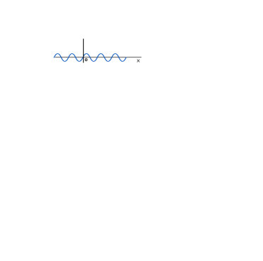
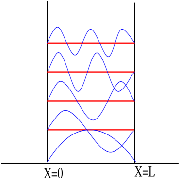
Figure 1.5: Free particle wave function (left), wave function in a compact space (right)

Thus it’s velocity will exceed the velocity of light in vacuum and lead to a problem: the tachyon state. So in this discussion we will consider a space-like co-ordinate as the extra dimension which will be compactified on a circle $S^{1}$ or $S^{1}/Z_{2}$ orbifold, for one extra-dimensional scenario, with radius of compactification R.

Before going into the more detailed discussion of extra dimensions let us recall the well known quantum mechanical one-dimensional box of size L. As we know, the solution of a particle moving along the $x$-direction with momentum $p$ is given by $\sim Ae^{ipx}+Be^{-ipx}$, here $x$ is infinitely long, $i.e$, the physical system is not compact and the particle momentum $p$ takes continuous values from $-\infty~{}{\rm to}~{}+\infty$. Let’s go to a bound system. Suppose the potential is infinite outside the box $0\leq x\leq\pi R$; $L=\pi R$ is the length of the box, while it is zero inside of the box. With the proper boundary condition that the wave function vanishes at the boundary, the solution takes the form $\psi=\sin{nx\over R}$ and the momentum of the particle is given by $p={n\over R}$, where $n$ can take any integer value. Due to the compactness of the $x$-dimension, the corresponding momentum $p_{x}$ becomes quantized. In the five-dimensional scenario where the extra space direction $y$ is compactified in a similar way, the corresponding quantized fifth component of momentum is given by $p_{5}={n\over R}$. Hence a particle which is massless in its zero mode, in the excited states, according to eqn.(1.148), acquire a mass $m_{n}={n\over R}$. This implies a large number of massive states whose mass is inversely proportional to the dimension of the box [18, 19].

1.8.1 Scalar particle in ED

In addition to the four space-time co-ordinates $x({\rm{\vec{x},t}})$, let us denote the extra space-type co-ordinate by $y$, compactified on a circle or radius R. Thus, the Lagrangian of a free complex scalar $\Phi(x,y)$with mass m will be a function of both $x~{}{\rm and}~{}y$ co-ordinates with a condition that the field at $y=2\pi R$ will match with that at $y=0$, $i.e$ it has a periodicity of $2\pi R$ along the $y$ direction. So one can expand it in a Fourier series as

$$\Phi(x,y)=\frac{1}{\sqrt{2\pi R}}\Phi_{0}(x)+\sum_{n=1}^{\infty}\frac{1}{\sqrt{\pi R}}\left[\Phi_{n}^{+}(x)\cos\left(\frac{ny}{R}\right)+\Phi_{n}^{-}(x)\sin\left(\frac{ny}{R}\right)\right].$$ (1.149)

The five-dimensional action is given by

$$S^{5}[\Phi]=\frac{1}{2}\int\!d^{4}x\ dy\ \left\{(\partial^{A}\Phi)^{\dagger}(\partial_{A}\Phi)-m^{2}\Phi^{\dagger}\Phi\right\}$$

with A = 0,1,2,3,5.

With the use of eqn.(1.149) if we replace the scalar field $\Phi$ and integrate out the extra dimension $y$ then the action will correspond to a large number Kaluza-Klein (KK) modes as

$$S^{4}[\Phi] = \frac{1}{2}\int\!d^{4}x\left\{(\partial^{\mu}\Phi_{0})^{\dagger}(\partial_{\mu}\Phi_{0})-m^{2}\Phi_{0}^{\dagger}\Phi_{0}\right\}+\sum_{n=1}^{\infty}\frac{1}{2}\int\!d^{4}x\left\{(\partial^{\mu}\Phi_{n}^{+})^{\dagger}(\partial_{\mu}\Phi_{n}^{+})-m_{n}^{2}{\Phi_{n}^{+}}^{\dagger}{\Phi_{n}^{+}}\right)$$ (1.150)

$$+ \sum_{n=1}^{\infty}\frac{1}{2}\int\!d^{4}x\left\{(\partial^{\mu}\Phi_{n}^{-})^{\dagger}(\partial_{\mu}\Phi_{n}^{-})-m_{n}^{2}{\Phi_{n}^{-}}^{\dagger}{\Phi_{n}^{-}}\right\},$$

where the n-th KK mode mass is given as

$${\rm m}_{n}^{2}={\rm m}^{2}+\frac{n^{2}}{R^{2}}.$$ (1.151)

In four-dimensional effective theory, thus, in addition to the zero mode field, we are getting two different sets – one is even and another odd under the transformation $y\rightarrow-y$ – of fields when the extra space dimension is compactified on the circle $S^{1}$.

1.8.2 Fermion particle in ED

In some models only the scalar bosons are allowed to access the extra dimensions while the fermions are kept in a fixed point of the extra dimension, called “brane”. In such cases the above compactification is quite natural but what happens if we intend to allow the fermions as well to access the extra dimension? Do we have the same set of Kaluza-Klein modes for the fermionic fields or something else?

Let us consider a fermion $\Psi$ in the five-dimensional field, where the extra space dimension is compactified the way we discussed in sec. 1.8.1. The five-dimensional spinor can be written as a two component four-dimensional spinor

$$\Psi=\left(\begin{array}[]{c}\psi_{R}\\ \psi_{L}\end{array}\right)~{}.$$ (1.154)

Note that in the five-dimensional field theory, one can construct the five $\Gamma^{A}$ matrices with A=0,1,2,3,5, from the usual four-dimensional ones as follows:

$$\Gamma^{\mu}=\gamma^{\mu}~{}~{}~{}{\rm and}~{}~{}\Gamma^{5}=i\gamma_{5}.$$ (1.155)

In 5d the fifth component of the $\Gamma^{A}$ is constructed from the $\gamma_{5}$ matrix, which is used, in four-dimensions, to define the chiral operator $P_{R/L}=(1\pm\gamma_{5})$. So, in five-dimensions, and it is true for any odd number of dimensions, there is no chiral operator. To be clear, in eqn.(1.154) the subscripts $L$ and $R$ are just two component notations only.

Like the scalar field discussion in sec. 1.8.1, let us consider the action for a massless fermion $\Psi$ as

$$S = \int~{}d^{4}xdy~{}~{}i\bar{\Psi}\Gamma^{A}\partial_{A}\Psi$$ (1.156)

$$= \int~{}d^{4}xdy~{}~{}\left(i\bar{\Psi}\gamma^{\mu}\partial_{\mu}\Psi+\bar{\Psi}\gamma^{5}\partial_{y}\Psi\right).$$

Due to the symmetry of the fermion field at the point $y=0$ and $y=2\pi R$, we can have the Fourier expansion of the field as

$$\psi_{L/R}(x,y)={1\over{\sqrt{2\pi R}}}\psi^{0}_{L/R}(x)+\sum_{n=1}^{\infty}{1\over{\sqrt{\pi R}}}\left\{\psi^{+n}_{L/R}(x)\cos\left({ny\over R}\right)+\psi^{-n}_{L/R}(x)\sin\left({ny\over R}\right)\right\}.$$ (1.157)

Once we put these fermions – eqn.(1.157) – in the above action eqn.(1.156) we end up with a few phenomenological problems.

For example, let us use the zero mode term in eqn.(1.157), then we have

$$S_{\rm zero~{}mode} = \int d^{4}x\int_{0}^{2\pi R}~{}dy~{}~{}\left({1\over{\sqrt{2\pi R}}}(\bar{\psi}^{0}_{L}+\bar{\psi}^{0}_{R})i\gamma^{\mu}\partial_{\mu}{1\over{\sqrt{2\pi R}}}(\psi^{0}_{L}+\psi^{0}_{R})\right).$$ (1.158)

$$\sim \int~{}d^{4}x\left\{\bar{\psi}^{0}_{L}i\gamma^{\mu}\partial_{\mu}\psi_{L}+\bar{\psi}^{0}_{R}i\gamma^{\mu}\partial_{\mu}\psi_{R}\right\}.$$

Thus, for each massless field in five-dimension we are having two massless zero modes in the four-dimensional effective theory. The four-dimensional fermion is thus vector like in nature. It is well-known that fermions in the SM are chiral in nature, the left chiral part transforms as a doublet under $SU(2)$ gauge transformation and the right chiral part transforms trivially. If the dimensional reduction doubles the state can we regain our chiral nature of the fermion in its zero mode?

To regain the chiral nature we have to compactify on an $S^{1}/Z_{2}$ orbifold instead of a circle. The expansions of different kind of field for the $S^{1}/Z_{2}$ orbifold will be discussed in sec. 2.3. In that case, although the higher KK modes of the chiral fermion behave as vector but the zero mode remains a chiral one.

1.8.3 Vector gauge bosons in ED

Let us consider a vector gauge boson $A_{M}$ with $M=0,1,2,3,5$ in five-dimensional scenario, where $A_{\mu}$ are the usual four vector bosons while the extra component $A_{5}$ will be a scalar. The Lagrangian of such a field is given by

$${{\cal L}}_{5d} = -{1\over 4}F_{MN}F^{MN}$$ (1.159)

where $F_{MN}=\partial_{M}A_{N}-\partial_{N}A_{M}$.

The compactification will be like in the two previous sections sec. 1.8.1 and sec. 1.8.2. In the same way, the periodicity of the field at $y=0$ and $y=2\pi R$ implies,

$$A_{M}(x,y)={1\over{\sqrt{2\pi R}}}A_{M}^{(0)}(x)+\sum_{n=1}{1\over{\sqrt{\pi R}}}\left\{A_{M}^{n}(x){\rm cos}\left({ny\over R}\right)+\tilde{A}_{M}^{n}(x){\rm sin}\left({ny\over R}\right)\right\}.$$ (1.160)

To discuss different components of an extra-dimensional vector gauge boson, let us assume a photon field in five-dimensional quantum electrodynamics (QED). In five dimensions this massless photon has five components. In the effective four-dimensional theory one should expect a tower of four-component photon fields and a tower of adjoint scalars. Although the zero mode of the photon has to be massless but the excitations for $n\not=0$ will be massive due to the KK contribution ($\sim n/R$). In QED there is no spontaneous symmetry breaking. The extra longitudinal degree of freedom for each of these massive KK gauge bosons will be obtained by absorbing the adjoint scalar of the same level. In five-dimensional QED, thus, we will have KK modes of the photon field only, but no KK modes of any adjoint scalar.

The corresponding SM scenario is quite complex. As besides the usual electroweak mass the weak gauge bosons acquired masses from the KK contribution also, so the usual unphysical components of the weak scalar doublet will no more be the Goldstone bosons. In reality, the KK modes of these unphysical fields will mix with the corresponding KK modes of ${W_{5}^{\pm}}_{n}$ and ${Z_{5}}_{n}$, to form three Goldstone modes $G^{0}_{n}$, $G^{\pm}_{n}$ and three physical scalar fields $a^{0}_{n}$ and $a^{\pm}_{n}$ [20]. With increasing KK number, the contributions of ${W_{5}^{\pm}}_{n}$ and ${Z_{5}}_{n}$ dominate the Goldstone boson modes while the unphysical components of the weak scalar doublet will, now, become main part of three physical scalar fields $a^{0}_{n}$ and $a^{\pm}_{n}$. In addition with these real scalars we will also have usual higgs boson $h$ and its KK excitations $h_{n}$.

Before going into the discussion of the universal extra dimension and the field expansion in the $S^{1}/Z_{2}$ orbifold let us have a brief discussion on how the large extra dimension scenario can explain the gauge hierarchy problem.

1.8.4 ADD model and solution of the gauge hierarchy problem

The main motivation of introducing extra dimensions into particle physics was to explain the huge hierarchy between the electroweak scale $\sim 100~{}{\rm GeV}$ and the Planck scale $\sim 10^{19}~{}{\rm GeV}$. The model we discuss in this subsection is the one of Large Extra Dimension (LED), introduced by Arkani-Hamed, Dimopoulos, Dvali (ADD) [21]. According to this model there exist $n$ extra spatial dimensions of radius $R$, which are accessed by only gravity while all other standard model particles are constrained at a particular point of these extra space dimensions. To fulfill the requirement it is assumed that the higher dimensional Planck mass $M_{Pl}^{(4+n)}$ is equal to the four-dimensional electroweak mass $m_{EW}$ thus evading the vexing hierarchy. Using Gauss’s law in $(4+n)$ dimensions, the gravitational potential between two masses ${\rm m}_{1}$ and ${\rm m}_{2}$ separated by a distance $r>>R$ is given by

$$V(r)\sim{{{\rm m}_{1}{\rm m}_{2}}\over{M_{Pl(4+n)}^{(n+2)}R^{n}}}{1\over r}.$$ (1.161)

Thus the four-dimensional effective $M_{Pl}$ is

$$M_{Pl}^{2}=M_{Pl(4+n)}^{2+n}R^{n}.$$ (1.162)

But, as stated above, our requirement is $M_{Pl(4+n)}~{}{\rm will~{}be}\sim{\rm m}_{EW}$. Thus replacing the same in the above eqn.(1.162), we have,

$$M_{Pl}^{2}={\rm m}_{EW}^{2+n}R^{n},$$ (1.163)

implies,

$$R\sim 10^{{30\over n}-17}cm\times\left({1{\rm TeV}\over{{\rm m}_{EW}}}\right)^{1+{2\over n}}.$$ (1.164)

Thus, the requirement that $M_{Pl}^{(4+n)}$ will be equal to the electroweak scale $\sim TeV$ implies $R=10^{13}$ cm for $n=1$, instantly excluded due to the huge deviation from Newtonian gravity.

At the time the model was proposed, Newtonian gravity was precisely checked upto 1mm. For $n=2$ from the above formula eqn.(1.164) we have $R=1$ mm. Thus models with at least two extra dimensions with a size of a millimeter can explain the gauge hierarchy problem.

1.8.5 Universal Extra Dimension

A model in which all the standard model particles are allowed to access the extra dimensions is known as the Universal Extra Dimension (UED) model also known as the ACD model after its proposers Appelquist, Cheng and Dobrescu [22].

Construction-wise it is very similar to the ADD model, but as in this case, in addition to gravity, scalars, fermions and vector gauge bosons are also accessing the extra dimension so, as discussed earlier, it should be compactified on an orbifold $S^{1}/Z_{2}$ instead of a circle. This orbifold is nothing but equivalent to the compactification on a circle of radius $R$ with a $Z_{2}$ symmetry - identifying $y\to-y$, where $y$ denotes the fifth compactified coordinate. The orbifolding is crucial in generating chiral zero modes for fermions.

The motivations of universal extra dimensions are quite speculative. Besides providing viable dark matter candidates the six-dimensional theory can explain from anomaly cancellation why we have only three generations [23]. Only three generation of fermions can remove the $SU(2)$ global gauge anomaly. Another good feature about universal extra dimensions is to provide a natural way to explain the long life time for the proton [24]. They could lead to a new mechanism of supersymmetry breaking [25], address the fermion mass hierarchy in an alternative way, provide a cosmologically viable dark matter candidate [26], stimulate power law renormalization group running [27, 28], admit substantial evolution of neutrino mixing angles defined through an effective Majorana neutrino mass operator [29], etc. The interesting point is that in this case the discrete symmetry which removes operators providing dangerous contributions to the proton decay is not imposed externally but is an essential ingredient for the theory.

With the compactification, as defined, on an orbifolding $S^{1}/Z_{2}$ for the five-dimensional scenario the expansion of the five-dimensional gauge bosons, scalars and fermions with the proper use of boundary conditions are given by

$$A_{\mu}(x,y) = \frac{\sqrt{2}}{\sqrt{2\pi R}}A_{\mu}^{(0)}(x)+\frac{2}{\sqrt{2\pi R}}\sum^{\infty}_{n=1}A_{\mu}^{(n)}(x)\cos\frac{ny}{R},~{}~{}~{}~{}A_{5}(x,y)=\frac{2}{\sqrt{2\pi R}}\sum^{\infty}_{n=1}A_{5}^{(n)}(x)\sin\frac{ny}{R},$$

$$\phi(x,y) = \frac{\sqrt{2}}{\sqrt{2\pi R}}\phi^{(0)}(x)+\frac{2}{\sqrt{2\pi R}}\sum^{\infty}_{n=1}\phi^{(n)}(x)\cos\frac{ny}{R},$$

$$\mathcal{Q}_{i}(x,y) = \frac{\sqrt{2}}{\sqrt{2\pi R}}\bigg{[}{\pmatrix{u_{i}\cr d_{i}}}_{L}(x)+\sqrt{2}\sum^{\infty}_{n=1}\Big{[}\mathcal{Q}^{(n)}_{iL}(x)\cos\frac{ny}{R}+\mathcal{Q}^{(n)}_{iR}(x)\sin\frac{ny}{R}\Big{]}\bigg{]},$$ (1.165)

$$\mathcal{U}_{i}(x,y) = \frac{\sqrt{2}}{\sqrt{2\pi R}}\bigg{[}u_{iR}(x)+\sqrt{2}\sum^{\infty}_{n=1}\Big{[}\mathcal{U}^{(n)}_{iR}(x)\cos\frac{ny}{R}+\mathcal{U}^{(n)}_{iL}(x)\sin\frac{ny}{R}\Big{]}\bigg{]},$$

$$\mathcal{D}_{i}(x,y) = \frac{\sqrt{2}}{\sqrt{2\pi R}}\bigg{[}d_{iR}(x)+\sqrt{2}\sum^{\infty}_{n=1}\Big{[}\mathcal{D}^{(n)}_{iR}(x)\cos\frac{ny}{R}+\mathcal{D}^{(n)}_{iL}(x)\sin\frac{ny}{R}\Big{]}\bigg{]},$$

where $i=1,2,3$ are generation indices. Above, $x(\equiv x^{\mu})$ denotes the first four coordinates, and as mentioned before, $y$ is the compactified coordinate. The complex scalar field $\phi(x,y)$ and the gauge boson $A_{\mu}(x,y)$ are $Z_{2}$ even fields with their zero modes identified with the SM scalar doublet and a SM gauge boson respectively. On the contrary, the field $A_{5}(x,y)$, which is a real scalar transforming in the adjoint representation of the gauge group, does not have any zero mode. The fields $\mathcal{Q}$, $\mathcal{U}$, and $\mathcal{D}$ describe the 5-dimensional quark doublet and singlet states, respectively, whose zero modes are identified with the 4-dimensional chiral SM quark states. The KK expansions of the weak-doublet and -singlet leptons will be likewise and are not shown for brevity.

Similar to the supersymmetric R-parity in this UED scenario we have Kaluza-Klein parity, in short KK-parity, which is conserved. This KK-parity is defined as

$$KK-{\rm parity}=(-1)^{n},$$ (1.166)

with $n$ as the KK number of the corresponding states. Thus in any KK-parity conserving process the lightest Kaluza-Klein particle (LKP) state, with $n=1$, cannot decay to the standard model particles and will be a good example of dark matter.

1.8.6 Bounds on the Universal Extra Dimension

During the discussion of LED scenario, we put some bound on the extra dimension based on the Newtonian gravitational interaction. In that case all the SM particles were constrained to be at a single point of the extra dimension so we did not care about the electro-weak or any other interactions. In the case UED scenario all the SM particles can access the extra dimensions. On the other hand weak interaction is perfectly measured up to a length $\sim{\rm m}_{EW}^{-1}$, much smaller than the LED bound 1mm, so we expect that the bound on the universal extra dimensions should be much more constraint. Constraints on this scenario from $g-2$ of the muon [30], flavour changing neutral currents [20, 31, 32], $Z\to b\bar{b}$ decay [33], the $\rho$ parameter [22, 34], other electroweak precision tests [35], implications from hadron collider studies [36], etc. imply that $R^{-1}~{}\raisebox{-1.72218pt}{\hbox to0.0pt{$\sim$\hss}}\raisebox{1.72218pt}{$>$}~{}300$ GeV. A recent inclusive $\bar{B}\to X_{s}\gamma$ analysis sets a stronger constraint $R^{-1}~{}\raisebox{-1.72218pt}{\hbox to0.0pt{$\sim$\hss}}\raisebox{1.72218pt}{$>$}~{}600$ GeV [37].

This thesis is devoted mainly to explore some of the distinctive characterisicts of new physics beyond the standard model. In chapter 2 we have presented the power law evolution of gauge, Yukawa and quartic couplings in the universal extra-dimensional scenario. We have also noted in this chapter that if supersymmetry is found at the LHC then UED will be out of reach of any future collider experiment. How the upper limit of the lightest supersymmetric neutral Higgs mass will be relaxed if supersymmetry is embeded in the extra dimension is discussed in chapter 3. In chapter 4, using three different approaches we have achieved a low intermediate left-right symmetry breaking scale in the supersymmetric $SO(10)$ Grand Unified Theory. Remaining within the SM in chapter 5 we have analysed the triquark state using $SU(6)$ unitary scalar factors and derived tree level pentquark masses. In chapter 6 we have presented the summary and conclusions of the work.

Chapter 2 Power law scaling in Universal Extra Dimension scenarios

2.1 Introduction

In section 1.6.3 we have seen that in the standard model, the gauge couplings (Yukawa and quartic scalar couplings as well) run logarithmically with the energy scale. The gauge couplings do not all meet at a point, they tend to unify near $10^{15}$ GeV. Such a high scale is beyond the reach of any present or future experiments. Instead of this logarithmic running, if the gauge couplings were running exponentially or with a definite power of energy then we could have a lower GUT scale. Extra dimensions is such a scenario which will lead to a power law running of the gauge couplings due to the large number of Kaluza-Klein states. Different KK modes will contribute the same way, as the zeroth mode does, to the gauge coupling evolution once we cross their corresponding threshold energies. The cumulative effect of this leads to a power law running of the gauge couplings.

Here we will work in a one UED scenario, where a flat extra dimension is compactified on an $S^{1}/Z_{2}$ orbifold as discussed earlier. With this compactification on an orbifolding $S^{1}/Z_{2}$ for the five-dimensional scenario the expansion of the five- dimensional gauge bosons, scalars and the fermions are already given in sec. 2.3. We examine the cumulative contribution of the KK states to the renormalisation group (RG) evolution of the gauge, Yukawa and quartic scalar couplings. Our motive, here, is to extract any subtle features that emerge due to the KK tower induced power law running of these couplings in contrast to the usual logarithmic running of the standard 4-dimensional theories, and whether they set any limit on parameters for the sake of theoretical and experimental consistency.

Let us now clarify the technical meaning of RG running in a higher dimensional context. This has been extensively discussed in [27] in a general context, and here we merely reiterate it to put our specific calculations into perspective. Like all other extra-dimensional models, from a 4-dimensional point of view, the UED scenario too is non-renormalisable due to the infinite multiplicity of the KK states. So $`$running’ of couplings as a function of the energy scale $E$ ceases to make sense. What we should say is that the couplings receive finite quantum corrections whose size depend on some explicit cutoff $\Lambda$. The corrections originate from the following number of KK states

$$\int^{\Lambda}_{1\over R}dn=R\int^{\Lambda}_{1\over R}dE=(\Lambda R-1)$$ (2.1)

which lie between the scale $R^{-1}$ where the first KK states are excited and the cutoff scale $\Lambda$. The couplings will have a power law dependence on $\Lambda$ as a result of the KK summation. This cutoff is interpreted as the scale where a paradigm shift occurs when some new renormalisable physics underlying our effective non-renormalisable framework surfaces.

2.2 Renormalisation Group Equations

We now lay out the strategy followed to compute the RG correction to the couplings from the KK modes. The first step is obviously the calculation of the contribution from a given KK level which has both $Z_{2}$-even and -odd states. Three points are noteworthy and should be taken into consideration during this step:

1. While the zero mode fermions are chiral as a result of orbifolding, the KK quarks and leptons at a given level are vector-like.

2. The fifth compotent of the gauge bosons are ($Z_{2}$ odd) scalars, but in the adjoint representation of the gauge group. Such states are not encountered in the SM context.

3. The KK index $n$ is conserved at each tree level vertex.

The first step KK excitation occurs at the scale $R^{-1}$ (modulo the zero mode mass). Up to this scale the RG evolution is logarithmic, controlled by the SM beta functions. Between $R^{-1}$ and $2R^{-1}$, the running is still logarithmic but with beta functions modified due to the first KK level excitations, and so on. Every time a KK threshold is crossed, new resonances are sparked into life, and new sets of beta functions rule till the next threshold arrives. The beta function contributions are the same for each of the $(\Lambda R-1)$ KK levels, which, in effect, can be summed. After this, the scale dependence is not logarithmic any more, it shows power law behaviour, as illustrated by Dienes et al in [39]. This illustration shows that if $\Lambda R\gg 1$, then to a very good accuracy the calculation basically boils down to computing the number of KK states up to the cutoff scale. For one extra dimension up to the energy scale $E$ this number is $S=ER$, and $E^{\rm max}=\Lambda$. Then if $\beta^{\rm SM}$ is a generic SM beta function valid during the logarithmic running up to $R^{-1}$, beyond that scale one should replace it as

$$\beta^{\rm SM}\to\beta^{\rm SM}+\Theta(E-\frac{1}{R})~{}(S-1)\tilde{\beta},$$ (2.2)

where $\tilde{\beta}$ is a generic contribution from a single KK level. The function $\Theta(E-\frac{1}{R})$ is used just to state that this UED $\beta$-function will only occur after an energy scale $E\geq{1\over R}$. Irrespective of whether we deal with the ‘running’ of gauge, Yukawa, or quartic scalar couplings, the structure of Eq. (2.2) would continue to hold. Clearly, the $S$ dependence reflects power law running. How this master formula (2.2) enters diagram by diagram into the evolution of the above couplings in the UED scenario constitutes the main part of calculation in this chapter.

2.2.1 Gauge couplings

While considering the evolution of the gauge couplings, we first write $\tilde{\beta}_{i}^{g}=\tilde{b}_{i}g_{i}^{3}$. The calculation of $\tilde{b}_{i}^{g}$ would proceed via the same set of Feynman graphs which give the SM contributions $b_{i}^{\rm SM}$ but now containing the KK internal lines. The key points to remember are the presence of adjoint scalars and doubling of KK quark and lepton states due to their vectorial nature.

Figure 2.1: Evolution of gauge couplings for UED with $R^{-1}$ = 1, 5, and 20 TeV. For each of the three couplings, $\alpha_{i}\equiv g_{i}^{2}/4\pi$.

We obtain

$$\tilde{b}_{1}=\frac{81}{10},~{}~{}\tilde{b}_{2}=\frac{7}{6},~{}~{}\tilde{b}_{3}=-\frac{5}{2},$$ (2.3)

where the $U(1)_{Y}$ beta function is appropriately normalised. Just to recall, the corresponding SM numbers are given in eqn.(1.126). We have plotted the evolution of gauge couplings in UED for $R^{-1}=$ 1, 5, and 20 TeV in Fig. 2.1. The running is fast, as expected, and the couplings nearly meet around 30, 138 and 525 TeV, respectively. It is not hard to provide an intuitive argument for such low unification scales and how they vary with $R$: roughly speaking, $\Lambda R$ is order $\ln(M_{\rm GUT}/M_{W})\sim\ln(10^{15})$, where $M_{\rm GUT}$ is the 4-dimensional GUT scale, i.e. the effect of a slow logarithmic running over a large scale is roughly reproduced by a fast power law sprint over a short track. The other striking feature reflected in Fig. 2.1 is that the $SU(2)$ gauge coupling ceases to be asymptotically free: the dominance of the KK matter sector over the gauge part in $\tilde{b}_{2}$ severely challenges the $SU(2)$ asymptotic freedom. In contrast, the negative sign of $\tilde{b}_{3}$ causes a precipitous drop in the $SU(3)$ gauge coupling with energy.

2.2.2 Yukawa couplings

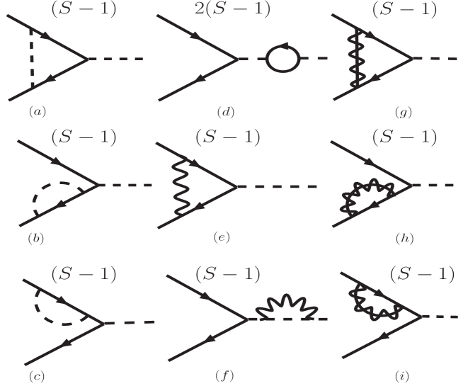
Figure 2.2: Diagrams contributing to Yukawa coupling evolution in the Landau gauge. Solid (broken) lines correspond to fermions (SM scalars), while wavy lines (wavy+solid lines) represent ordinary gauge bosons (fifth components of gauge bosons).

The Feynman diagrams that contribute to the power law evolution of Yukawa couplings (in Landau gauge) are shown in Fig. 2.2. The contributions come from the pure SM states, their KK towers, and from the adjoint representation scalars. The last two contributions, as the master formula (2.2) indicates, have an overall proportionality factor $(S-1)$. As we examine contributions from individual KK states, we see that due to the argument of fermion chirality, not in all diagrams do the cosine and sine mode states both simultaneously contribute. This accounts for a relative factor of 2 between the two types of diagrams. For example, in Fig. 2.2a the fermionic KK modes can only come from cosine expansions, whereas in Fig. 2.2d both cosine and sine fermion modes contribute. This is why Fig. 2.2a has a multiplicating factor $(S-1)$, while for Fig. 2.2d the factor is $2(S-1)$. Whereever $A_{5}$ is involved as an internal line, the associated KK internal fermions necessarily come from sine expansion, e.g. in Figs. 2.2g, 2.2h and 2.2i. The above book-keeping has been done for individual graphs and the proportionality factors have been mentioned for each diagram in Fig. 2.2. The Yukawa RG equations (beyond the threshold $R^{-1}$) can be written as ($t=\ln E$):

$$16\pi^{2}\frac{dy_{f}}{dt}=\beta^{\rm SM}_{y_{f}}+\Theta(E-\frac{1}{R})~{}\beta^{\rm UED}_{y_{f}},$$ (2.4)

Figure 2.3: Evolution of the top quark Yukawa coupling in the UED scenario (left panel) and (b) the SM (right panel). UED evolution is shown for three different values of $R^{-1}$ and the curves are terminated at the corresponding unification scales.

where $f$ generically stands for the up/down quarks or leptons. The SM beta functions $\beta^{\rm SM}_{y_{f}}$ can be found e.g. in [40].

The UED contributions to the beta functions $\beta^{\rm UED}_{y_{l,u,d}}$ are given by: $\displaystyle\beta^{\rm UED}_{y_{l}}$ $\displaystyle=$ $\displaystyle(S-1)\;\left[-(\frac{21}{8}g_{2}^{2}+\frac{129}{40}g_{1}^{2})+\frac{3}{2}y_{l}^{2}\right]\;y_{l}+2(S-1)\;\left[Y_{l}+3Y_{u}+3Y_{d}\right]\;y_{l},$ $\displaystyle\beta^{\rm UED}_{y_{u}}$ $\displaystyle=$ $\displaystyle(S-1)\;\left[-(12g_{3}^{2}+\frac{21}{8}g_{2}^{2}+\frac{9}{8}g_{1}^{2})+\frac{3}{2}(y_{u}^{2}-y_{d}^{2})\right]\;y_{u}+2(S-1)\;\left[Y_{l}+3Y_{u}+3Y_{d}\right]\;y_{u},$ (2.5) $\displaystyle\beta^{\rm UED}_{y_{d}}$ $\displaystyle=$ $\displaystyle(S-1)\;\left[-(12g_{3}^{2}+\frac{21}{8}g_{2}^{2}+\frac{9}{40}g_{1}^{2})+\frac{3}{2}(y_{d}^{2}-y_{u}^{2})\right]\;y_{d}+2(S-1)\;\left[Y_{l}+3Y_{u}+3Y_{d}\right]\;y_{d},$ with $Y_{l}=\sum_{l}y_{l}^{2}$, $Y_{d}=\sum_{d}y_{d}^{2}$, and $Y_{u}=\sum_{u}y_{u}^{2}$. To illustrate how the power law dependence of Yukawa couplings quantitatively compares and contrasts with their 4-dimensional logarithmic running, we have exhibited in Fig. 2.3 the behaviour of the top-quark Yukawa coupling in the two cases.

Another consequence of unification in many models is a prediction of the low energy value of $m_{b}/m_{\tau}$. This ratio, unity at the unification scale, at low energies takes the values 4.7, 4.2, and 3.9 for $1/R$ = 1, 5, and 20 TeV, respectively. Admittedly, $m_{b}$ is on the high side; a limitation which perhaps may be attributable to the one-loop level of the calculation.

2.2.3 Quartic scalar coupling and the Higgs mass

The one-loop diagrams through which the KK modes contribute to the power law running of the quartic scalar coupling $\lambda$ (in Landau gauge) are shown in Fig. 2.4. As clarified before in the case of Yukawa running, the extra factor of 2 in front of $(S-1)$ for some graphs indicates that cosine and sine KK modes both contribute only to those graphs. The evolution equation can be written as

$$16\pi^{2}\frac{d\lambda}{dt}=\beta^{\rm SM}_{\lambda}+\Theta(E-\frac{1}{R})~{}\beta^{\rm UED}_{\lambda}$$ (2.6)

The expressions for $\beta^{\rm SM}_{\lambda}$ can be found e.g. in [41]. The UED beta functions are given by $\displaystyle\beta^{\rm UED}_{\lambda}$ $\displaystyle=$ $\displaystyle(S-1)\left[3g_{2}^{4}+\frac{6}{5}g_{2}^{2}g_{1}^{2}+\frac{9}{25}g_{1}^{4}-3\lambda(3g_{2}^{2}+\frac{3}{5}g_{1}^{2})+12\lambda^{2}\right]$ (2.7) $\displaystyle+$ $\displaystyle 2(S-1)\left[4\left(Y_{l}+3Y_{u}+3Y_{d}\right)\lambda-4\sum_{l,u,d}\left(y_{l}^{4}+3y_{u}^{4}+3y_{d}^{4}\right)\right].$

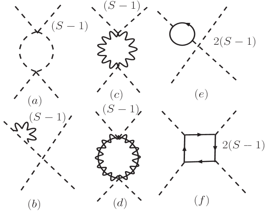
Figure 2.4: Diagrams contributing to quartic scalar coupling evolution. The conventions are the same as in Fig. 2.2.

Figure 2.5: Bounds on the Higgs mass at the electroweak scale in the UED scenario from the triviality and vacuum stability conditions for $R^{-1}$ = 1, 5, and 20 TeV. See text for details.

The evolution of $\lambda$ has interesting bearings on the Higgs mass. In the standard 4-dimensional context, bounds on the Higgs mass have been placed on the grounds of ‘triviality’ and ‘vacuum stability’ [42]. What do they imply in the UED context? The ‘triviality’ argument requires that $\lambda$ stays away from the Landau pole, i.e. remains finite, all the way to the cutoff scale $\Lambda$. The condition that $1/\lambda(\Lambda)>0$ can be translated to an upper bound on the Higgs mass ($m_{H}$) at the electroweak scale when the cutoff of the theory is $\Lambda$. This has been plotted in Fig. 2.5 (the upper curves) for three different values of $R$. A given point on that curve (for a given $R$) corresponds to a maximum allowed $m_{H}$ at the weak scale; for a larger $m_{H}$ the coupling $\lambda$ becomes infinite at some scale less than $\Lambda$ and the theory ceases to be perturbative. Clearly, this $m_{H}^{\rm max}$ varies as we vary the cutoff $\Lambda$ . The argument of ‘vacuum stability’ relies on the requirement that the scalar potential be always bounded from below, i.e. $\lambda(\Lambda)>0$. This can be translated to a lower bound $m_{H}^{\rm min}$ at the weak scale. The lower set of curves in Fig. 2.5 (for three values of $R^{-1}$) represent the ‘vacuum stability’ limits, the region below the curve for a given $R$ being ruled out. Recalling that the cutoff is where the gauge couplings tend to unify, we observe that the Higgs mass is limited in the narrow zone

$$148~{}\raisebox{-1.72218pt}{\hbox to0.0pt{$\sim$\hss}}\raisebox{1.72218pt}{$<$}~{}m_{H}~{}\raisebox{-1.72218pt}{\hbox to0.0pt{$\sim$\hss}}\raisebox{1.72218pt}{$<$}~{}186~{}{\rm GeV}$$ (2.8)

in all the three cases, for a zero mode top quark mass of 174.2 GeV. Admittedly, our limits are based on one-loop corrections only. That the upper and lower limits are insensitive to the choice of $R$ is not difficult to understand, as what really counts is the number of KK states, given by the product $\Lambda R$, which, as mentioned before, is nearly constant, order $\ln(10^{15})$. The limits in Eq. (2.8) are very close to what we obtain in the SM at the one-loop level, namely $147~{}\raisebox{-1.72218pt}{\hbox to0.0pt{$\sim$\hss}}\raisebox{1.72218pt}{$<$}~{}m_{H}^{\rm SM}~{}\raisebox{-1.72218pt}{\hbox to0.0pt{$\sim$\hss}}\raisebox{1.72218pt}{$<$}189$ GeV (see also [43], where one-loop SM results have been derived).

2.2.4 Supersymmetric UED

What happens if we take the supersymmetric (SUSY) version of UED? A 5-dimensional $N=1$ supersymmetry when perceived from a 4-dimensional context contains two different $N=1$ multiplets forming one $N=2$ supermultiplet. For a comprehensive analysis, we refer the readers to [27]. There are two issues that immediately concern our analysis. First, unlike in the non-SUSY case, the Higgs scalar in a chiral multiplet will now have both even and odd $Z_{2}$ modes on account of degrees of freedom counting consistent with supersymmetry. Also, there will be two such $N=2$ chiral supermultiplets to meet the requirement of supersymmetry. Second, in the RG evolution two energy scales will come into play. The first of these is the supersymmetry scale, called $M_{S}$, which we take to be 1 TeV. Beyond $M_{S}$, supersymmetric particles get excited and their contributions must be included in the RG evolution. The second scale is that of the compactified extra dimension $1/R$, which we take to be larger than $M_{S}$.

The gauge coupling evolution must now be specified for three different regions. The first of these is when $E<M_{S}$ where the SM with the additional scalar doublet beta functions are in control. In this region:

$${b}_{1o}=\frac{21}{5},~{}~{}{b}_{2o}=-\frac{10}{3},~{}~{}{b}_{3o}=-7.$$ (2.9)

Once $M_{S}$ is crossed and up until $1/R$, we also have the superpartners of the SM particles pitching in with their effects. The contributions of the SM particles and their superpartners together are given by:

$${b}_{1s}=\frac{33}{5},~{}~{}{b}_{2s}=1,~{}~{}{b}_{3s}=-3.$$ (2.10)

Finally, when the KK-modes are excited ($E>1/R$) one has further contributions from the individual modes:

$$\tilde{b}_{1}=\frac{66}{5},~{}~{}\tilde{b}_{2}=10,~{}~{}\tilde{b}_{3}=6.$$ (2.11)

Thus, beyond $1/R$, the total contribution is given by

$$b_{i}^{\rm tot}=b_{io}+\Theta(E-M_{S})~{}(b_{is}-b_{i0})+\Theta(E-\frac{1}{R})~{}(S-1)~{}\tilde{b}_{i},$$ (2.12)

Not unexpectedly, for the SUSY UED case, gauge unification is possible. We observe that the introduction of this plethora of KK excitations of the SM particles and their superpartners radically changes the beta functions; so much so, that the gauge couplings tend to become non-perturbative before unification is achieved. For clarity, we make the argument more explicit below. First, from Eqs. (2.10) and (2.11) we note that the dominance of the KK matter over the KK gauge parts is so overwhelming that the $SU(3)$ beta function ($\tilde{b}_{3}$) beyond the first KK threshold ceases to be negative any longer. The other two gauge beta functions, which were already positive with contributions from zero mode particles plus their superpartners, become even more positive. So the curves for all the three gauge couplings would have the same sign slopes once the KK modes are excited. As a result, with increasing energy the three curves for $\alpha_{g}^{-1}$ would dip with a power law scaling fast into a region where the couplings themselves become too large at the time they meet. Therefore, in order that all of them remain perturbative during the entire RG evolution, the onset of the KK dynamics has to be sufficiently delayed. This requirement imposes $R^{-1}~{}\raisebox{-1.72218pt}{\hbox to0.0pt{$\sim$\hss}}\raisebox{1.72218pt}{$>$}~{}5.0\times 10^{10}$ GeV. In effect, this implies that the twin requirements of a SUSY-UED framework as well as perturbative gauge coupling unification pushes the detectability of the KK excitations well beyond the realm of the LHC.

2.3 Conclusions and Outlook

As the LHC is getting all set to roar in 2008, expectations are mounting as we prepare ourselves to get a glimpse of new and unexplored territory. New physics of different incarnations, especially supersymmetry and/or extra dimensions, are crying out for verification. How does the landscape beyond the electroweak scale confront the evolution of the gauge, Yukawa and scalar quartic couplings? Will there be a long logarithmic march through the desert all the way to $10^{(16-17)}$ GeV, or is a power law sprint awaiting us with a stamp of extra dimensions? In which way does the latter quantitatively differ from the former has been the subject of our investigation in the present chapter. We observe the following landmarks that characterise the extra-dimensional running:

1. The orbifolding renders some subtle features to the RG running in UED. Due to the conservation of KK number at tree level vertices, the $Z_{2}$ even and odd KK states selectively contribute to different diagrams. While some diagrams are forbidden, there are new diagrams originating from adjoint scalar exchanges. In the present chapter we have performed a diagram by diagram book-keeping leading to the evolution equations.

2. Low gauge coupling unification scales can be achieved without introducing non-perturbative gauge couplings. The unification scale depends on $R$, and is approximately given by $\Lambda\sim(25-30)/R$.

3. The ‘triviality’ and ‘vacuum stability’ bounds on the Higgs mass have been studied in the context of power law evolution. This limits the Higgs mass in the range $148~{}\raisebox{-1.72218pt}{\hbox to0.0pt{$\sim$\hss}}\raisebox{1.72218pt}{$<$}m_{H}~{}\raisebox{-1.72218pt}{\hbox to0.0pt{$\sim$\hss}}\raisebox{1.72218pt}{$<$}186$ GeV at the one-loop level. The corresponding SM limits at the one-loop level are not very different.

4. If low energy SUSY is realised in Nature, then the requirement of perturbative gauge coupling unification pushes the inverse radius of compactification all the way up to $\sim 10^{10}$ GeV. Thus if superpartners of the SM particles are observed at the LHC, the nearest KK states within the UED framework are predicted to lie beyond the boundary of any observational relevance.

It should be admitted that even if TeV scale extra-dimensional theories are established, the spectrum might be more complicated than what UED predicts. The confusion is expected to clear up at least when the low-lying KK states face appointment with destiny within the first few years of the LHC run. Our intention in the present chapter has been to choose a simple framework to study power law evolution. Flat extra-dimensional models are particularly handy as they provide equispaced KK states which allow an elegant handling of internal KK summation in the loops. UED is an ideal test-bed to conduct this study as it has been motivated from various angles and subjected to different phenomenological tests.

Chapter 3 Extra-dimensional relaxation of the upper limit of the lightest supersymmetric neutral Higgs mass

3.1 Introduction

The most general symmetries of local relativistic quantum field theories include supersymmetry, briefly discussed in sec.-1.7, a phenomenological version [14] of which is awaiting a final judgement within the next few years as the LHC turns on. Indeed, one of the most coveted targets of the LHC is to capture the Higgs boson, and supersymmetry, admitting chiral fermions together with their scalar partners in the same representations, tacitly provides a rationale for treating the Higgs as an elementary object [16]. Furthermore, through the removal of the quadratic divergence that plagues the ordinary Higgs mass, phenomenological supersymmetry has emerged as a leading candidate of physics beyond the standard model. A key signature of the minimal version of supersymmetry is that the lightest Higgs boson mass obeys an upper bound $\sim$ 135 GeV, see sec.-3.2.2, – a prediction which will be put to test during the LHC run. Now, supersymmetry is an integral part of string theory which attempts to provide a quantum picture of all interactions. Since string theory is intrinsically a higher dimensional theory, a reanalysis of some 4-dimensional (4d) supersymmetric wisdom in the backdrop of extra dimensions might provide important clues to our search strategies. As we know the main motivation of LHC is to find the Higgs boson besides examining the new physics. In this chapter we address the following question which we believe is extremely timely: What is the upper limit of the lightest CP-even neutral Higgs mass if the minimal supersymmetric standard model (MSSM) is embedded in extra dimensions [44]? We consider the embedding first in one and then in two extra dimensions.

Let us first discuss why this is an important issue. Recall that MSSM has two Higgs doublet superfields ($H_{1}$ and $H_{2}$), and supersymmetry does not allow the scalar potential to have independent quartic couplings. Gauge interactions generate them through supersymmetry breaking $D$-terms and the effective quartic interactions are written in terms of the gauge couplings. This makes the Higgs spectrum partially predictive, in the sense that at the tree level the lightest neutral Higgs ($h$) weighs less than ${\rm m}_{Z}$ (${\rm m}_{h}^{2}<{\rm m}_{Z}^{2}\cos^{2}2\beta$, where $\tan\beta$ is the ratio of two vacuum expectation values (VEVs)), see sec.-3.2.1. However, ${\rm m}_{h}$ receives quantum corrections, see sec.-3.2.2, which, due to the large top quark Yukawa coupling and for heavy stop squarks, can become as large as $\Delta{\rm m}_{h}^{2}\sim(3G_{F}{\rm m}_{t}^{4}/\sqrt{2}\pi^{2})\ln({\rm m}_{\tilde{t}}^{2}/{\rm m}_{t}^{2})$, where ${\rm m}_{\tilde{t}}$ is an average stop squark mass [45, 46]. The upper limit on ${\rm m}_{h}$ is then pushed to around 135 GeV for squark mass in the ${\cal{O}}$(TeV) range. Notice that the non-observation of the Higgs boson at LEP2 has already set a lower limit ${\rm m}_{h}>114.5$ GeV [47, 48], which is satisfied only if a sizable quantum correction elevates the Higgs mass beyond the tree level upper limit of ${\rm m}_{Z}$. This implies (i) lower values of $\tan\beta$, which is usually chosen in the range $1<\tan\beta<{\rm m}_{t}/{\rm m}_{b}$, are disfavoured, and (ii) the squark mass ${\rm m}_{\tilde{t}}$ has to be in the TeV range, which also sets the scale of a generic soft supersymmetry breaking mass $M_{S}$. The MSSM prediction of a light Higgs is also in line with the indication coming from electroweak precision tests that the neutral Higgs should weigh below 199 GeV [49]. The so called ‘little hierarchy’ problem then arises out of an order of magnitude mass splitting between the Higgs and the superparticles.

Adding a gauge singlet superfield ($N$) in the MSSM spectrum and coupling it with $H_{1,2}$ via the superpotential $\lambda NH_{1}H_{2}$ helps to ease the tension. Not only does this next to minimal version of supersymmetry (the so called NMSSM [50]) help to address the ‘$\mu$ problem’, it also generates a tree level quartic coupling in the scalar potential which modifies the tree level upper limit on ${\rm m}_{h}$ through ${\rm m}_{h}^{2}<{\rm m}_{Z}^{2}\cos^{2}2\beta[1+2\lambda^{2}\tan^{2}2\beta/(g^{2}+g^{\prime 2})]$ (see [51]). Assuming $\lambda$ to be in the perturbative regime, i.e., $\lambda\sim g,g^{\prime}$, one basically obtains a new contribution $\sim{\rm m}_{Z}^{2}\sin^{2}2\beta$ to the tree level ${\rm m}_{h}^{2}$. This way the low $\tan\beta$ regime can be revived. Since many supersymmetric couplings depend on $\tan\beta$, search strategies alter in a significant way if the disfavoured low $\tan\beta$ region is thus resurrected^,.

In this chapter we adopt a different approach which also revives the low $\tan\beta$ region. We stick to the MSSM particle content, but embed it in a higher dimension compactified at the inverse TeV scale [27]. Although we argued in the beginning that string theory provides a rationale for linking the two ideas, namely, supersymmetry and extra dimension, establishing any rigourous connection between the two at the level of phenomenological models is still a long shot. Here we take a $`$bottom-up’ approach: we first outline what has already been studied in the phenomenological context of TeV scale extra-dimensional scenarios, and then illustrate what we aim to achieve in this chapter.

1. As in the previous chapter, we will discuss the physics with one extra dimension first (with inverse radius of compactification around a TeV) but without supersymmetry and later for completeness we will also glance at the scenario with two extra dimensions. A typical model is the one UED scenario where all particles access the extra dimension. Constraint, in general, on this scenario, discussed in the sec-1.8.6, is $R^{-1}~{}\raisebox{-1.72218pt}{\hbox to0.0pt{$\sim$\hss}}\raisebox{1.72218pt}{$>$}~{}300$ GeV while a recent inclusive $\bar{B}\to X_{s}\gamma$ analysis sets a stronger constraint $R^{-1}~{}\raisebox{-1.72218pt}{\hbox to0.0pt{$\sim$\hss}}\raisebox{1.72218pt}{$>$}~{}600$ GeV [37].

2. Our object of interest is a supersymmetric theory (e.g. MSSM) but embedded in a higher dimension. Here we ask the following question: What would be the shift in the Higgs mass due to radiative effects induced by extra dimensions? The kind of scenario, here, we will consider is not the exact UED scenario but a modified universal extra dimension (mUED) where the SM bosons along with their superpartners access the higher dimensional bulk in addition with only one generation (here, the third one) of the SM fermions together with their superpartners. From a 4d perspective, all the states which access the bulk will have Kaluza-Klein (KK) towers. The zero modes, i.e., those states which do not have any momenta along the extra coordinates, are identified with the standard 4d MSSM spectra. Now, not only the top quark and the stop squarks would contribute to the radiative correction to $m_{h}^{2}$, their KK partners would do so as well. As it turns out, the radiative correction driven by the KK states has the same sign as the one from the zero modes. As a result, $\Delta{\rm m}_{h}^{2}$ becomes larger and thus the upper limit on ${\rm m}_{h}$ is pushed to higher values beyond the usual 4d MSSM limit of around 135 GeV. As we shall see, in the absence of any left-right scalar mixing, the new contribution coming from KK modes is to a good approximation proportional to $R^{2}({\rm m}_{\tilde{t}}^{2}-{\rm m}_{t}^{2})/n^{2}$. This fits our intuition that the KK contribution falls with higher KK modes and vanishes both when $R\to 0$ and in the limit of exact supersymmetry. We can interpret the result in two ways. Either, we take large $\tan\beta$ and ${\cal{O}}$(TeV) squark mass that yielded the 4d supersymmetry limit $\sim$ 135 GeV, in which case the new upper limit shoots up by several tens of GeV. Or, we may admit lower $\tan\beta$ and/or accommodate lighter zero mode squarks which were hitherto disfavoured in the 4d context. Either way, the Higgs phenomenology gets an interesting twist which is intuitively comprehensible and analytically tractable, owing largely due to the fact that we are here dealing with only one additional parameter, namely, the radius of compactification. Moreover, the top quark mass which appears with fourth power in the expression of $\Delta{\rm m}_{h}^{2}$ is now known to a precision better than ever (${\rm m}_{t}=170.9\pm 1.8$ GeV [54]).

As mentioned before, we have considered the embedding of 4d supersymmetry in one as well as two extra dimensions. We shall see that qualitatively the KK contributions to the radiative corrections of ${\rm m}_{h}$ from 5d and 6d theories are similar, the quantitative estimates differ due to the different density of KK states in the two cases. In 5d, the KK states are spaced as $n/R$ (modulo their zero mode masses) where $n$, an integer, is the KK number, whereas in 6d, a similar expression holds except $n^{2}\Rightarrow j^{2}+k^{2}$, where $j$ and $k$ are two different sets of KK numbers corresponding to the two compactified directions.

Section 3.2 is basically a review of the standard derivation of the upper limit of the lightest neutral Higgs in conventional 4d MSSM in the effective potential approach. This paves the way, in the next section, to upgrade the above derivation for accommodating contributions from the KK modes of the top quark and squarks in 5d and 6d scenarios. In section 3.4, we shall comment on the numerical impact of the higher KK modes on the lightest neutral Higgs mass and its consequences. We shall draw our conclusion in the final section of the chapter.

3.2 MSSM and the neutral Higgs spectrum

3.2.1 Tree level mass relations

Let us start with the discussion what we started in sec.-1.7 that in supersymmetry we have two complex scalar doublets as

$${H_{1}}=\left(\begin{array}[]{c}{H_{1}}^{0}\\ {H_{1}}^{-}\end{array}\right),~{}~{}~{}~{}~{}{H_{2}}=\left(\begin{array}[]{c}{H_{2}}^{+}\\ {H_{2}}^{0}\end{array}\right),$$ (3.5)

whose $SU(2)\times U(1)$ quantum numbers are (2,$-$1) and (2,$+$1) respectively. $H_{1}^{0}$ couples with down-type quarks and charged leptons, while $H_{2}^{0}$ couples with up-type quarks. This guarantees natural suppression of flavour-changing neutral currents in the limit of exact supersymmetry. Now, out of the eight degrees of freedom contained in the two Higgs doublets three are absorbed as the longitudinal modes of the $W$ and the $Z$ bosons, while the remaining five modes appear as physical states. Of these five states, two are charged $(H^{\pm})$ and three are neutral ($h,H,A$). Our present concern is the neutral sector of which ($h,H$) are CP-even, while $A$ is CP-odd.

The tree level potential involving these two doublets is given by

$$V=m_{1}^{2}|H_{1}|^{2}+m_{2}^{2}|H_{2}|^{2}+m_{12}^{2}(H_{1}H_{2}+{\rm h.c})+{1\over 8}g_{2}^{2}(H_{2}^{\dagger}\sigma^{a}H_{2}+H_{1}^{\dagger}\sigma^{a}H_{1})^{2}+{1\over 8}{g_{1}}^{2}(|H_{2}|^{2}-|H_{1}|^{2})^{2},$$ (3.6)

where ${\rm m}_{1}^{2}$, ${\rm m}_{2}^{2}$ and ${\rm m}_{12}^{2}$ are soft supersymmetry breaking mass parameters, $g_{2}$ and $g_{1}$ are the $SU(2)$ and $U(1)$ gauge couplings, and $\sigma^{a}$ $(a=1,2,3)$ are the Pauli matrices. Note that the quartic coupling is related to the gauge couplings. The part involving the neutral fields is given by

$$V_{0}={\rm m}_{1}^{2}|H_{1}^{0}|^{2}+{\rm m}_{2}^{2}|H_{2}^{0}|^{2}-{\rm m}_{12}^{2}(H_{1}^{0}H_{2}^{0}+{\rm h.c})+{1\over 8}(g_{2}^{2}+g_{1}^{2})(|H_{1}^{0}|^{2}-|H_{2}^{0}|^{2})^{2}.$$ (3.7)

After spontaneous symmetry breaking the minimum of $V_{0}$ involves the following two VEVs: $\langle H_{1}^{0}\rangle=v_{1}$ and $\langle H_{2}^{0}\rangle=v_{2}$. The combination $v=\sqrt{v_{1}^{2}+v_{2}^{2}}=(\sqrt{2}G_{F})^{-1/2}\simeq 246$ GeV sets the Fermi scale. Let us define shifted neutral Higgs fields as

$$H_{1}^{0}\rightarrow H_{1}^{0}+{1\over{\sqrt{2}}}(S_{1}+iP_{1})$$ (3.8)

$$H_{2}^{0}\rightarrow H_{2}^{0}+{1\over{\sqrt{2}}}(S_{2}+iP_{2})$$

The mass matrix square for the CP-odd sector is given by

$$\cal{M}_{\rm Im}^{\rm 2} = {{{\partial}^{\rm 2}V}\over{{\partial}P_{\rm i}{\partial}P_{\rm j}}}$$ (3.9)

$$= \left(\begin{array}[]{cc}{\rm m}_{1}^{2}+{1\over 4}(g_{1}^{2}+g_{2}^{2})(v_{1}^{2}-v_{2}^{2})&{\rm m}_{12}^{2}\\ {\rm m}_{12}^{2}&{\rm m}_{2}^{2}-{1\over 4}(g_{1}^{2}+g_{2}^{2})(v_{1}^{2}-v_{2}^{2})\end{array}\right)={\rm m}^{2}_{12}\left(\begin{array}[]{cc}{v_{2}\over v_{1}}&1\\ 1&{v_{1}\over v_{2}}\end{array}\right).$$ (3.14)

As it is a singular matrix, so one of the eigenvalues will be zero which is the mass of the neutral massless Goldstone boson $G^{0}$

$${\rm m}_{G^{0}}=0$$ (3.16)

while other one is the CP-odd Higgs boson $A$ whose mass simply is given by the $`$ trace’ of the matrix as

$${\rm m}_{A}^{2} = \frac{2{\rm m}_{12}^{2}}{\sin 2\beta}~{}$$ (3.17)

where,

$${\sin 2\beta}={{2v_{1}v_{2}}\over{v_{1}^{2}+v_{2}^{2}}}.$$ (3.18)

The CP-even neutral sector mass is

$$\cal{M}_{\rm Re}^{\rm 2}={{{\partial}^{\rm 2}V}\over{{\partial}S_{\rm i}{\partial}S_{\rm j}}}=\left(\begin{array}[]{cc}2{\rm m}_{1}^{2}+{1\over 2}(g_{1}^{2}+g_{2}^{2})(3v_{1}^{2}-v_{2}^{2})&-2{\rm m}_{12}^{2}-(g_{1}^{2}+g_{2}^{2})v_{1}v_{2}\\ -2{\rm m}_{12}^{2}-(g_{1}^{2}+g_{2}^{2})v_{1}v_{2}&2{\rm m}_{1}^{2}+{1\over 2}(g_{1}^{2}+g_{2}^{2})(3v_{2}^{2}-v_{1}^{2})\end{array}\right)$$ (3.21)

and we get CP-even neutral Higgs masses as

$${\rm m}^{2}_{h,H} = {1\over 2}\left[{\rm m}_{A}^{2}+{\rm m}_{Z}^{2}\mp\sqrt{({\rm m}_{A}^{2}+{\rm m}_{Z}^{2})^{2}-4{\rm m}_{A}^{2}{\rm m}_{Z}^{2}\cos^{2}2\beta}\right],$$ (3.22)

where, by definition, $h$ is the lighter of the two CP-even Higgs.

Using these relations we can have a useful sum rule just by adding $m_{h}^{0}$ and $m_{H}^{0}$ from eqn.-(3.22)

$${\rm m}_{h}^{2}+{\rm m}_{H}^{2}={\rm m}_{A}^{2}+{\rm m}_{Z}^{2}.$$ (3.23)

On the otherhand, from eqn.(3.22), we have

$${\rm m}^{2}_{H} = {1\over 2}\left[({\rm m}_{A}^{2}+{\rm m}_{Z}^{2})+({\rm m}_{A}^{2}+{\rm m}_{Z}^{2})\left\{1-{{4{\rm m}_{A}^{2}{\rm m}_{Z}^{2}\cos^{2}2\beta}\over{({\rm m}_{A}^{2}+{\rm m}_{Z}^{2})^{2}}}\right\}^{1\over 2}\right],$$

$$= {\rm m}_{A}^{2}+{\rm m}_{Z}^{2}-{{{\rm m}_{A}^{2}{\rm m}_{Z}^{2}\cos^{2}2\beta}\over{{\rm m}_{A}^{2}+{\rm m}_{Z}^{2}}}.$$

Thus we have,

$${\rm m}^{2}_{H}={\rm m}_{A}^{2}+{\rm m}_{Z}^{2}\left\{1-{{\cos^{2}2\beta}\over{1+{{\rm m}_{Z}^{2}\over{{\rm m}_{A}^{2}}}}}\right\},~{}~{}{\rm implies,}~{}~{}{\rm m}^{2}_{H}>{\rm m}^{2}_{A}$$ (3.25)

or,

$${\rm m}^{2}_{H}={\rm m}_{Z}^{2}+{\rm m}_{A}^{2}\left\{1-{{\cos^{2}2\beta}\over{1+{{\rm m}_{A}^{2}\over{{\rm m}_{Z}^{2}}}}}\right\},~{}~{}{\rm implies,}~{}~{}{\rm m}^{2}_{H}>{\rm m}^{2}_{Z}.$$ (3.26)

Again, just by multiplying $m_{h}^{0}$ with $m_{H}^{0}$ from eqn.-(3.22) we have,

$${\rm m}^{2}_{h}{\rm m}^{2}_{H}={\rm m}_{Z}^{2}{\rm m}_{A}^{2}{\cos^{2}2\beta}.$$ (3.27)

So, we have the relation,

$${\rm m}^{2}_{h}={{\rm m}_{A}^{2}\over{\rm m}^{2}_{H}}{\rm m}_{Z}^{2}{\cos^{2}2\beta}~{}~{}{\rm implies,}~{}~{}{\rm m}^{2}_{h}<{\rm m}_{Z}^{2}{\cos^{2}2\beta}<{\rm m}_{Z}^{2},~{}~{}{\rm since,}~{}~{}{\rm m}^{2}_{H}>{\rm m}^{2}_{A};$$ (3.28)

and,

$${\rm m}^{2}_{h}={{\rm m}_{Z}^{2}\over{\rm m}^{2}_{H}}{\rm m}_{A}^{2}{\cos^{2}2\beta}~{}~{}{\rm implies,}~{}~{}{\rm m}^{2}_{h}<{\rm m}_{A}^{2}{\cos^{2}2\beta}<{\rm m}_{A}^{2},~{}~{}{\rm since,}~{}~{}{\rm m}^{2}_{H}>{\rm m}^{2}_{Z}.$$ (3.29)

Thus, finally, in the tree level we have the inequality

$${\rm m}_{h}\leq{\rm min}~{}({\rm m}_{A},{\rm m}_{Z})|\cos 2\beta|\leq{\rm min}~{}({\rm m}_{A},{\rm m}_{Z}),$$ (3.30)

i.e., at the tree level (i) the lighter of the two CP-even Higgs ($h$) weighs less than ${\rm m}_{Z}$, and (ii) the CP-odd Higgs ($A$) is heavier than $h$ but lighter than $H$.

3.2.2 Radiative corrections

We shall now discuss how the above tree level relations are affected by quantum loops [45, 46]. We shall confine our discussion on the correction to ${\rm m}_{h}$ only, and that too at the one-loop level. We note two important points:

1. Radiative corrections to ${\rm m}_{h}$ are dominated by the top quark Yukawa coupling ($h_{t}$) and the masses of the stop squarks ($\tilde{t}_{1}$, $\tilde{t}_{2}$). For large values of $\tan\beta$, the contributions from the $b$-quark sector also assume significance. We shall ignore loop contributions mediated by lighter quarks or the gauge bosons.

2. The tree level Higgs mass is protected by supersymmetry. In the limit of exact supersymmetry, the entire quantum correction vanishes. So radiative corrections to ${\rm m}_{h}$ will be controlled by $M_{S}$.

Three different approaches have been adopted in the literature to calculate the radiative corrections to ${\rm m}_{h}$: (i) effective potential technique, (ii) direct diagrammatic calculations, and (iii) renormalisation group (RG) method, assuming $M_{S}\gg{\rm m}_{Z}$ and fixing the quartic coupling proportional to $(g^{2}+g^{\prime 2})$ at that scale and then evolving down to weak scale. In this chapter, we shall follow the effective potential approach primarily for the sake of conveniently including the effect of new physics later.

We first start with an RG-improved tree level potential $V_{0}(Q)$ which contains running masses ${\rm m}_{i}^{2}(Q)$ and running gauge couplings $g_{i}(Q)$. The full one-loop effective potential is now given by

$$V_{1}(Q)=V_{0}(Q)+\Delta V_{1}(Q),$$ (3.31)

where, in terms of the field dependent masses $M(H)$,

$$\Delta V_{1}(Q)={1\over{64\pi^{2}}}{\rm Str}M^{4}(H)\left\{\ln{M^{2}(H)\over{Q^{2}}}-{3\over 2}\right\}.$$ (3.32)

The $Q$-dependence of $\Delta V_{1}(Q)$ cancels against that of $V_{0}(Q)$ making $V_{1}(Q)$ independent of $Q$ up to higher loop orders. The supertrace in Eq. (3.32), defined through

$${\rm Str}f({\rm m}^{2})=\sum_{i}(-1)^{2J_{i}}(2J_{i}+1)f({\rm m}_{i}^{2}),$$ (3.33)

has to be taken over all members of a supermultiplet and where ${\rm m}_{i}^{2}\equiv{\rm m}_{i}^{2}(H)$ is the field-dependent mass eigenvalue of the particle $i$ with spin $J_{i}$. As an example, the contribution from the chiral multiplet containing the top quark and squarks is given by

$$\Delta V_{t}={3\over{32\pi^{2}}}\left\{{\rm m}_{\tilde{t}_{1}}^{4}\left(\ln{{\rm m}_{\tilde{t}_{1}}^{2}\over{Q^{2}}}-{3\over 2}\right)+{\rm m}_{\tilde{t}_{2}}^{4}\left(\ln{{\rm m}_{\tilde{t}_{2}}^{2}\over{Q^{2}}}-{3\over 2}\right)-2{\rm m}_{t}^{4}\left(\ln{{\rm m}_{t}^{2}\over{Q^{2}}}-{3\over 2}\right)\right\},$$ (3.34)

where the overall factor of 3 comes from colour. Note that ${\rm m}_{\tilde{t}_{i}}$ and ${\rm m}_{t}$ in Eq. (3.34) are field dependent masses. Even though $h_{b}\ll h_{t}$, the contribution from the bottom supermultiplet turns out to be numerically significant in the large $\tan\beta$ region. $\Delta V_{b}$ can be written analogously to $\Delta V_{t}$ with the appropriate replacements of top and stop masses by bottom and sbottom masses respectively.

We now explicitly write down the field dependent mass terms. This simply means a replacement of $v_{i}$ by $H_{i}^{0}$ ($i=1,2$) wherever $v_{i}$ appear in the expression of masses. The field dependent top and bottom quark masses are given by

$${\rm m}_{t}^{2}(H)=h_{t}^{2}|H_{2}^{0}|^{2}~{};~{}{\rm m}_{b}^{2}(H)=h_{b}^{2}|H_{1}^{0}|^{2}.$$ (3.35)

The field dependent stop and sbottom squark mass matrices are written as

$${M_{\tilde{t}}^{2}}(H)=\left(\begin{array}[]{cc}{\rm m}_{Q}^{2}+h_{t}^{2}|H^{0}_{2}|^{2}&h_{t}(A_{t}H^{0}_{2}+\mu{H_{1}^{0}}^{*})\\ h_{t}(A_{t}{H^{0}_{2}}^{*}+\mu H_{1}^{0})&{\rm m}_{U}^{2}+h_{t}^{2}|H^{0}_{2}|^{2}\end{array}\right),$$ (3.38)

and

$${M_{\tilde{b}}^{2}}(H)=\left(\begin{array}[]{cc}{\rm m}_{Q}^{2}+h_{b}^{2}|H^{0}_{1}|^{2}&h_{b}(A_{b}H^{0}_{1}+\mu{H_{2}^{0}}^{*})\\ h_{b}(A_{b}{H^{0}_{1}}^{*}+\mu H_{2}^{0})&{\rm m}_{D}^{2}+h_{b}^{2}|H^{0}_{1}|^{2}\end{array}\right).$$ (3.41)

In Eqs. (3.38) and (3.41) ${\rm m}_{Q}$, ${\rm m}_{U}$ and ${\rm m}_{D}$ are soft supersymmetry breaking masses, $A_{t}$ and $A_{b}$ are trilinear soft supersymmetry breaking mass dimensional couplings, and $\mu$ is the supersymmetry preserving mass dimensional parameter connecting $H_{1}$ and $H_{2}$ in the superpotential. We take both trilinear and the $\mu$ couplings to be real. We have neglected the $D$-term contributions which are small, being proportional to gauge couplings. The squark masses appearing in Eq. (3.34) are obtained from the diagonalisation of Eq. (3.38).

We now consider the radiative correction to the CP-odd scalar mass matrix. The one-loop corrected mass matrix square, obtained by taking double derivatives of the full potential with respect to the pseudo-scalar excitations, can be written as

$${\cal{M}}^{2}_{({\rm odd})}=\left(\begin{array}[]{cc}{\rm tan}\beta&1\\ 1&{\rm cot}\beta\end{array}\right)({\rm m}_{12}^{2}+\Delta).$$ (3.44)

The radiative corrections generated as a consequence of supersymmetry breaking are contained in $\Delta=\Delta^{\rm t}+\Delta^{\rm b}$, which is given by

$$\Delta^{\rm t(b)}=-{3\over{32\pi^{2}}}{h_{t(b)}^{2}\mu A_{t(b)}\over\left[{{\rm m}^{2}_{{\tilde{t}_{1}}({\tilde{b}_{1}})}-{\rm m}^{2}_{{\tilde{t}_{2}}({\tilde{b}_{2}})}}\right]}\left[f\left({\rm m}^{2}_{{\tilde{t}_{1}}({\tilde{b}_{1}})}\right)-f\left({\rm m}^{2}_{{\tilde{t}_{2}}({\tilde{b}_{2}})}\right)\right]$$ (3.45)

where

$$f({\rm m}^{2})=2{\rm m}^{2}\left(\ln{{\rm m}^{2}\over{Q^{2}}}-1\right).$$ (3.46)

The zero eigenvalue corresponds to the massless Goldstone boson which is eaten by the $Z$ boson. The massive state is the pseudo-scalar $A$ whose radiatively corrected mass square is given by

$${\rm m}_{A}^{2}=\frac{2({\rm m}_{12}^{2}+\Delta)}{\sin 2\beta}.$$ (3.47)

The $Q$-dependence of ${\rm m}_{A}$ cancels in Eq. (3.47) up to one-loop order. In any case, we shall treat the radiatively corrected ${\rm m}_{A}$ as an input parameter.

Now we are all set to calculate the radiative corrections in the neutral CP-even mass eigenvalues. The one-loop corrected mass matrix square is obtained by taking double derivatives of the full potential with respect to the scalar excitations and is given by

$${\cal{M}}^{2}_{({\rm even})}=\left(\begin{array}[]{cc}{\rm m}_{Z}^{2}\cos^{2}\beta+{\rm m}_{A}^{2}\sin^{2}\beta&-({\rm m}_{A}^{2}+{\rm m}_{Z}^{2})\sin\beta\cos\beta\\ -({\rm m}_{A}^{2}+{\rm m}_{Z}^{2})\sin\beta\cos\beta&{\rm m}_{Z}^{2}\sin^{2}\beta+{\rm m}_{A}^{2}\cos^{2}\beta\end{array}\right)+{3\over{4\pi^{2}v^{2}}}\left(\begin{array}[]{cc}\Delta_{11}&\Delta_{12}\\ \Delta_{12}&\Delta_{22}\end{array}\right),$$ (3.52)

where $\Delta_{ij}=\Delta^{\rm t}_{ij}+\Delta^{\rm b}_{ij}$. The individual $\Delta_{ij}$’s are explicitly written below:

$$\Delta_{11}^{t} = {{\rm m}_{t}^{4}\over{{\sin}^{2}\beta}}\left(\mu(A_{t}+\mu{\rm cot}\beta)\over{{\rm m}_{\tilde{t}_{1}}^{2}-{\rm m}_{\tilde{t}_{2}}^{2}}\right)^{2}g({\rm m}_{\tilde{t}_{1}}^{2},m_{\tilde{t}_{2}}^{2}),$$

$$\Delta_{12}^{t} = {{\rm m}_{t}^{4}\over{{\sin}^{2}\beta}}{\mu(A_{t}+\mu{\cot}\beta)\over{{\rm m}_{\tilde{t}_{1}}^{2}-{\rm m}_{\tilde{t}_{2}}^{2}}}\left[{\ln}{{{\rm m}_{\tilde{t}_{1}}^{2}}\over{{\rm m}_{\tilde{t}_{2}}^{2}}}+{A_{t}(A_{t}+\mu{\cot}\beta)\over{{\rm m}_{\tilde{t}_{1}}^{2}-{\rm m}_{\tilde{t}_{2}}^{2}}}g({\rm m}_{\tilde{t}_{1}}^{2},{\rm m}_{\tilde{t}_{2}}^{2})\right],$$

$$\Delta_{22}^{t} = {{\rm m}_{t}^{4}\over{\sin^{2}\beta}}\left[\ln{{{\rm m}_{\tilde{t}_{1}}^{2}}{{\rm m}_{\tilde{t}_{2}}^{2}}\over{{\rm m}_{t}^{4}}}+{2A_{t}(A_{t}+\mu{\cot}\beta)\over{{\rm m}_{\tilde{t}_{1}}^{2}-{\rm m}_{\tilde{t}_{2}}^{2}}}{\ln}{{{\rm m}_{\tilde{t}_{1}}^{2}}\over{{\rm m}_{\tilde{t}_{2}}^{2}}}+\left(A_{t}(A_{t}+\mu{\cot}\beta)\over{{\rm m}_{\tilde{t}_{1}}^{2}-{\rm m}_{\tilde{t}_{2}}^{2}}\right)^{2}g({\rm m}_{\tilde{t}_{1}}^{2},{\rm m}_{\tilde{t}_{2}}^{2})\right],$$

$$\Delta_{11}^{b} = {{\rm m}_{b}^{4}\over{{\cos}^{2}\beta}}\left[{\ln}{{{\rm m}_{\tilde{b}_{1}}^{2}}{{\rm m}_{\tilde{b}_{2}}^{2}}\over{{\rm m}_{b}^{4}}}+{2A_{b}(A_{b}+\mu{\tan}\beta)\over{{\rm m}_{\tilde{b}_{1}}^{2}-{\rm m}_{\tilde{b}_{2}}^{2}}}{\ln}{{{\rm m}_{\tilde{b}_{1}}^{2}}\over{\rm m}_{\tilde{b}_{2}}^{2}}+\left(A_{b}(A_{b}+\mu\tan\beta)\over{{\rm m}_{\tilde{b}_{1}}^{2}-{\rm m}_{\tilde{b}_{2}}^{2}}\right)^{2}g({\rm m}_{\tilde{b}_{1}}^{2},{\rm m}_{\tilde{b}_{2}}^{2})\right],$$

$$\Delta_{12}^{b} = {{\rm m}_{b}^{4}\over{{\cos}^{2}\beta}}{\mu(A_{b}+\mu{\tan}\beta)\over{{\rm m}_{\tilde{b}_{1}}^{2}-{\rm m}_{\tilde{b}_{2}}^{2}}}\left[{\ln}{{{\rm m}_{\tilde{b}_{1}}^{2}}\over{{\rm m}_{\tilde{b}_{2}}^{2}}}+{A_{b}(A_{b}+\mu{\tan}\beta)\over{{\rm m}_{\tilde{b}_{1}}^{2}-{\rm m}_{\tilde{b}_{2}}^{2}}}g({\rm m}_{\tilde{b}_{1}}^{2},{\rm m}_{\tilde{b}_{2}}^{2})\right],$$ (3.53)

$$\Delta_{22}^{b} = {{\rm m}_{b}^{4}\over{{\cos}^{2}\beta}}\left(\mu(A_{b}+\mu{\tan}\beta)\over{{\rm m}_{\tilde{b}_{1}}^{2}-{\rm m}_{\tilde{b}_{2}}^{2}}\right)^{2}g({\rm m}_{\tilde{b}_{1}}^{2},{\rm m}_{\tilde{b}_{2}}^{2}).$$

where

$$g({\rm m}_{1}^{2},{\rm m}_{2}^{2})=2-{{{\rm m}_{1}^{2}+{\rm m}_{2}^{2}}\over{{\rm m}_{1}^{2}-{\rm m}_{2}^{2}}}\ln{{\rm m}_{1}^{2}\over{\rm m}_{2}^{2}}.$$ (3.54)

Two points deserve mention at this stage:

1. While the leading log contribution appears in $\Delta_{22}$ for the top sector, the same appears in $\Delta_{11}$ for the bottom sector. This happens because the right-handed top quark couples to $H_{2}$ while the right-handed bottom quark couples to $H_{1}$. In the absence of any left-right scalar mixing, these leading logs are the only radiative contributions.

2. Ignoring the left-right scalar mixing, the radiative shift to the Higgs mass square coming from the top-stop sector turns out to be $\Delta{\rm m}_{h}^{2}=(3/4\pi^{2}v^{2})\Delta^{t}_{22}\sin^{2}\beta\sim(3{\rm m}_{t}^{4}/2\pi^{2}v^{2})\ln({\rm m}_{\tilde{t}}^{2}/{\rm m}_{t}^{2})$, where ${\rm m}_{\tilde{t}}=\sqrt{{\rm m}_{\tilde{t}_{1}}{\rm m}_{\tilde{t}_{2}}}$ is an average stop mass. This is the expression we quoted in the Introduction.

3.3 Radiative corrections due to extra dimensions

We now discuss the supersymmetric version of the theory. A 5d $N=1$ supersymmetry from a 4d perspective appears as two $N=1$ supersymmetries forming an $N=2$ theory. For the details of the hypermultiplet structures of this theory, we refer the readers to [27]. Our concern in this chapter is to calculate the radiative contribution to ${\rm m}_{h}$ coming from the KK partners of particles and superparticles. We now proceed through the following steps.

1. Let us first recall that the $N=2$ supersymmetry prohibits any bulk Yukawa interaction involving three chiral multiplets. The Yukawa interaction is considered to be localised at a brane, like $-(h_{t5}/\Lambda^{3/2})\int d^{4}x~{}\int dy~{}\delta(y)\int d^{2}\theta~{}({\cal{H}}_{2}{\cal{Q}}{\cal{T}}~{}+~{}{\rm h.c.})$, where the residual supersymmetry is that of $N=1$, $h_{t5}$ is a dimensionless Yukawa coupling in 5d and $\Lambda$ the cutoff scale. This localisation has a consequence in the counting of KK degrees of freedom that contribute to the Higgs mass radiative correction. The delta function ensures that those fields which accompany the sine function after Fourier decomposition do not sense the Yukawa interaction.

2. As in the case of 4d (zero mode) supersymmetry, here too the dominant effect arises solely from the third generation quark superfields, only that now we have to include the contributions from their KK towers. We shall continue to ignore contributions from the gauge interactions or those from the first two quark families, as they are not numerically significant. As we are working in the mUED scenario, where only one generation accesses the bulk and the other two are confined to a brane, then the validity of the theory extends further, allowing even a perturbative gauge coupling unification, we checked, around $E\sim 40/R$. The five-dimensional Fourier decomposition of the corresponding superfields from the eqn. (1.8.5).

3. In our scheme $M_{S}$ and $R$ are independent parameters, although we take them to be of the same order. Towards the end of sec-3.4, we briefly remark on the numerical implications of any possible connection between $M_{S}$ and $R$.

4. The KK equivalent of Eq. (3.34), which captures the KK contribution arising from the top quark chiral hypermultiplet, is then given by

   $$\Delta V_{t}^{n}={3\over{32\pi^{2}}}\left[{\rm m}_{\tilde{t}_{1}^{n}}^{4}\left(\ln{{\rm m}_{\tilde{t}_{1}^{n}}^{2}\over{Q^{2}}}-{3\over 2}\right)+{\rm m}_{\tilde{t}_{2}^{n}}^{4}\left(\ln{{\rm m}_{\tilde{t}_{2}^{n}}^{2}\over{Q^{2}}}-{3\over 2}\right)-2{\rm m}_{t^{n}}^{4}\left(\ln{{\rm m}_{t^{n}}^{2}\over{Q^{2}}}-{3\over 2}\right)\right],$$ (3.55)

   where the field dependent KK masses are given by ${\rm m}_{\tilde{t}_{1}^{n}}^{2}={\rm m}_{\tilde{t}_{1}}^{2}+n^{2}/R^{2}$, ${\rm m}_{\tilde{t}_{2}^{n}}^{2}={\rm m}_{\tilde{t}_{2}}^{2}+n^{2}/R^{2}$, and ${\rm m}_{t^{n}}^{2}={\rm m}_{t}^{2}+n^{2}/R^{2}$. The field dependence is hidden inside the zero mode masses, as illustrated in Eqs. (3.35), (3.38) and (3.41). The corresponding contribution triggered by the bottom quark hypermultiplet, $\Delta V_{b}^{n}$, can be written mutatis mutandis.

5. We now calculate the KK loop contribution to the neutral scalar mass matrix. The procedure will be exactly the same as that followed for the 4d MSSM scenario in the previous section. Since we are going to treat the radiatively corrected physical ${\rm m}_{A}$ as an input parameter, we concentrate only on the CP-even mass matrix. We first take another look at the expressions of the different $\Delta_{ij}$, assembled in Eq. (3.2.2), calculated in the context of the 4d MSSM. The prefactors like ${\rm m}_{t}^{4}$ or ${\rm m}_{b}^{4}$ originated by the action of double differentiation on the field dependent squark or quark masses. Recall that the squark and quark masses are (quadratically) separated by the soft supersymmetry breaking mass-squares which are not field dependent. So, irrespective of whether we double-differentiate the squark or quark masses we get either the top or bottom quark Yukawa coupling. In the same way, the KK mass-squares are separated from the zero mode mass-squares by a field independent quantity $n^{2}/R^{2}$. Therefore, the expressions for $(\Delta_{ij})^{n}$, the radiative corrections from the $n$th KK level, continue to have the zero mode quark masses ${\rm m}_{t}^{4}$ or ${\rm m}_{b}^{4}$ as prefactors, but now the arguments of the other functions contain the corresponding KK masses.

We are now all set to write down the expressions for different $(\Delta_{ij})^{n}$ for $n\neq 0$. They are given by

$$(\Delta_{11}^{t})^{n} = {{\rm m}_{t}^{4}\over{{\rm sin}^{2}\beta}}\left(\mu(A_{t}+\mu{\rm cot}\beta)\over{{\rm m}_{\tilde{t}_{1}^{n}}^{2}-{\rm m}_{\tilde{t}_{2}^{n}}^{2}}\right)^{2}g({\rm m}_{\tilde{t}_{1}^{n}}^{2},{\rm m}_{\tilde{t}_{2}^{n}}^{2}),$$

$$(\Delta_{12}^{t})^{n} = {{\rm m}_{t}^{4}\over{\sin^{2}\beta}}{\mu(A_{t}+\mu\cot\beta)\over{{\rm m}_{\tilde{t}_{1}^{n}}^{2}-{\rm m}_{\tilde{t}_{2}^{n}}^{2}}}\left[\ln{{{\rm m}_{\tilde{t}_{1}^{n}}^{2}}\over{{\rm m}_{\tilde{t}_{2}^{n}}^{2}}}+{A_{t}(A_{t}+\mu\cot\beta)\over{{\rm m}_{\tilde{t}_{1}^{n}}^{2}-{\rm m}_{\tilde{t}_{2}^{n}}^{2}}}g({\rm m}_{\tilde{t}_{1}^{n}}^{2},{\rm m}_{\tilde{t}_{2}^{n}}^{2})\right],$$

$$(\Delta_{22}^{t})^{n} = {{\rm m}_{t}^{4}\over{{\rm sin}^{2}\beta}}\left[{\ln}{{{\rm m}_{\tilde{t}_{1}^{n}}^{2}}{{\rm m}_{\tilde{t}_{2}^{n}}^{2}}\over{{\rm m}_{t^{n}}^{4}}}+{2A_{t}(A_{t}+\mu\cot\beta)\over{{\rm m}_{\tilde{t}_{1}^{n}}^{2}-{\rm m}_{\tilde{t}_{2}^{n}}^{2}}}\ln{{{\rm m}_{\tilde{t}_{1}^{n}}^{2}}\over{{\rm m}_{\tilde{t}_{2}^{n}}^{2}}}+\left(A_{t}(A_{t}+\mu\cot\beta)\over{{\rm m}_{\tilde{t}_{1}^{n}}^{2}-{\rm m}_{\tilde{t}_{2}^{n}}^{2}}\right)^{2}g({\rm m}_{\tilde{t}_{1}^{n}}^{2},{\rm m}_{\tilde{t}_{2}^{n}}^{2})\right],$$

$$(\Delta_{11}^{b})^{n} = {{\rm m}_{b}^{4}\over{{\rm cos}^{2}\beta}}\left[\ln{{{\rm m}_{\tilde{b}_{1}^{n}}^{2}}{{\rm m}_{\tilde{b}_{2}^{n}}^{2}}\over{{\rm m}_{b^{n}}^{4}}}+{2A_{b}(A_{b}+\mu\tan\beta)\over{{\rm m}_{\tilde{b}_{1}^{n}}^{2}-{\rm m}_{\tilde{b}_{2}^{n}}^{2}}}\ln{{{\rm m}_{\tilde{b}_{1}^{n}}^{2}}\over{{\rm m}_{\tilde{b}_{2}^{n}}^{2}}}+\left(A_{b}(A_{b}+\mu\tan\beta)\over{{\rm m}_{\tilde{b}_{1}^{n}}^{2}-{\rm m}_{\tilde{b}_{2}^{n}}^{2}}\right)^{2}g({\rm m}_{\tilde{b}_{1}^{n}}^{2},{\rm m}_{\tilde{b}_{2}^{n}}^{2})\right],$$

$$(\Delta_{12}^{b})^{n} = {{\rm m}_{b}^{4}\over{\cos^{2}\beta}}{\mu(A_{b}+\mu\tan\beta)\over{{\rm m}_{\tilde{b}_{1}^{n}}^{2}-{\rm m}_{\tilde{b}_{2}^{n}}^{2}}}\left[\ln{{{\rm m}_{\tilde{b}_{1}^{n}}^{2}}\over{{\rm m}_{\tilde{b}_{2}^{n}}^{2}}}+{A_{b}(A_{b}+\mu\tan\beta)\over{{\rm m}_{\tilde{b}_{1}^{n}}^{2}-{\rm m}_{\tilde{b}_{2}^{n}}^{2}}}g({\rm m}_{\tilde{b}_{1}^{n}}^{2},{\rm m}_{\tilde{b}_{2}^{n}}^{2})\right],$$ (3.56)

$$(\Delta_{22}^{b})^{n} = {{\rm m}_{b}^{4}\over{\cos^{2}\beta}}\left(\mu(A_{b}+\mu\tan\beta)\over{{\rm m}_{\tilde{b}_{1}^{n}}^{2}-{\rm m}_{\tilde{b}_{2}^{n}}^{2}}\right)^{2}g({\rm m}_{\tilde{b}_{1}^{n}}^{2},{\rm m}_{\tilde{b}_{2}^{n}}^{2}).$$

Now we have to add the $(\Delta^{t})^{n}$ and $(\Delta^{b})^{n}$ matrices to the one-loop corrected (from zero modes only) mass matrix in Eq. (3.52), sum over $n$, and then diagonalise to obtain the eigenvalues ${\rm m}_{h}^{2}$ and ${\rm m}_{H}^{2}$. The KK radiative corrections decouple in powers of $(R^{2}/n^{2})$. To provide intuition to the expressions in Eq. (3.3), we display below the approximate formulae for $(\Delta^{t})^{n}$ in leading powers of $(R^{2}/n^{2})$:

$$(\Delta_{11}^{t})^{n} = -\frac{1}{6}\left(\frac{R^{4}}{n^{4}}\right)\frac{{\rm m}_{t}^{4}}{\sin^{2}\beta}\left[\mu(A_{t}+\mu\cot\beta)\right]^{2},$$

$$(\Delta_{12}^{t})^{n} = \left(\frac{R^{2}}{n^{2}}\right)\frac{{\rm m}_{t}^{4}}{\sin^{2}\beta}\mu(A_{t}+\mu\cot\beta),$$ (3.57)

$$(\Delta_{22}^{t})^{n} = \left(\frac{R^{2}}{n^{2}}\right)\frac{{\rm m}_{t}^{4}}{\sin^{2}\beta}\left[({\rm m}_{\tilde{t}_{1}}^{2}+{\rm m}_{\tilde{t}_{2}}^{2}-2{\rm m}_{t}^{2})+2A_{t}(A_{t}+\mu\cot\beta)\right].$$

Similar expressions for $(\Delta^{b})^{n}$ can be written, with appropriate replacements like ${\rm m}_{t}\leftrightarrow{\rm m}_{b}$, $\cot\beta\leftrightarrow\tan\beta$, etc. So, in the absence of any left-right scalar mixing, the KK contribution to $\Delta{\rm m}_{h}^{2}$ is controlled by $R^{2}({\rm m}^{2}_{\tilde{t}}-{\rm m}_{t}^{2})/n^{2}$ and its higher powers.

Six-dimensional scenario:  For the 6d scenario we follow the compactification on a chiral square, as done in [58], which admits zero mode chiral fermions. The two extra spatial coordinates $(y_{1},y_{2})$ are compactified on a square of side length $L$, such that $0<y^{1},~{}y^{2}<\pi R(\equiv L)$. The boundary condition is the identification of the two pairs of adjacent sides of the squares such that the values of a field at two identified points differ by a phase ($\theta$). Nontrivial solutions exist when $\theta$ takes four discrete values $(n\pi/2)$ for $n=0,1,2,3$ and the zero modes appear when $n=0$. What matters to our calculation in this chapter is the structure of the KK masses, a generic pattern of which is given by

$${\rm m}_{j,k}^{2}={\rm m}_{0}^{2}+\frac{j^{2}+k^{2}}{R^{2}},$$ (3.58)

where $j,k$ are integers such that $j\geq 0$ and $k\geq 0$. We display in Table 3.1 the KK mass spectrum (neglecting the zero mode mass ${\rm m}_{0}$ for simplicity of presentation while in the actual calculation we do keep it). The formalism we developed for 5d will simply go through for 6d. More concretely, the structure of Eqs. (3.55) and (3.3) would remain the same in 6d, only that one should now read $n\Rightarrow(j,k)$. The numerical impact in the two cases obviously differ, as we shall witness in the next section.

$(j,k)$	$1,0$	(1,1)	(2,0)	(2,1) or (1,2)	(2,2)	(3,0)	(3,1) or (1,3)	(3,2) or (2,3)	(4,0)
${\rm m}_{j,k}$	1	$\sqrt{2}$	2	$\sqrt{5}$	$2\sqrt{2}$	3	$\sqrt{10}$	$\sqrt{13}$	4

Table 3.1: 6d scenario mass spectrum in $(1/R)$ units, neglecting the zero mode mass.

3.4 Results

In this section we explore the consequences of the extra-dimensional contributions to the Higgs mass encoded in the exact one-loop expressions in Eq. (3.3). But to start with, to get a feel for the numerical impact of the extra dimensions, consider the scenario pared down to its bare minimum by assuming that left-right scalar mixing ingredients are vanishing, i.e., $\mu=A_{t}=A_{b}=0$. This leads to two degenerate stop squarks: ${\rm m}_{\tilde{t}}^{2}=M_{S}^{2}+{\rm m}_{t}^{2}$. Then, for a moderate $\tan\beta$,

$$\Delta{\rm m}_{h}^{2}~{}(n=0)\sim\frac{3{\rm m}_{t}^{4}}{2\pi^{2}v^{2}}\ln\left(1+\frac{M_{S}^{2}}{{\rm m}_{t}^{2}}\right);~{}~{}~{}\Delta{\rm m}_{h}^{2}~{}(n\neq 0)\sim\frac{3{\rm m}_{t}^{4}}{2\pi^{2}v^{2}}\frac{(M_{S}R)^{2}}{n^{2}}.$$ (3.59)

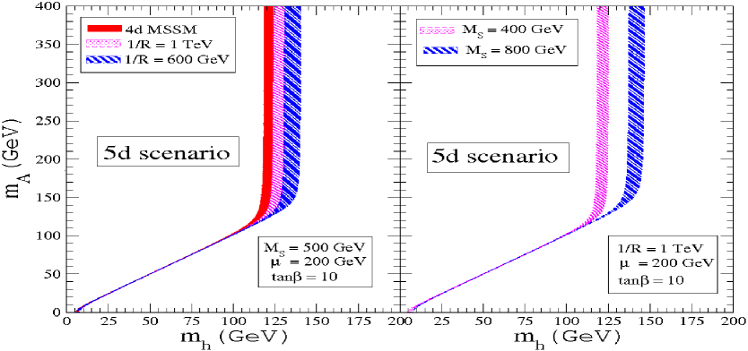
Figure 3.1: The variation of ${\rm m}_{h}$ with ${\rm m}_{A}$ in the 5d MSSM for different choices of the supersymmetry breaking scale ($M_{S}$) and the compactification radius ($R$). The width of each band corresponds to the variation of $A_{t}$ and $A_{b}$ in the range $(0.8-1.2)M_{S}$ (see text).

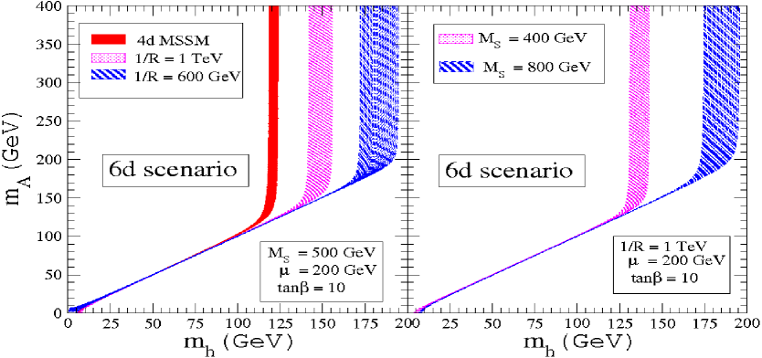
Figure 3.2: As in Fig. 3.1 but for the 6d MSSM.

Indeed, non-zero trilinear and $\mu$ terms would complicate the expressions, yet Eq. (3.59) provides a good intuitive feel for our results displayed through the different plots. The expected decoupling of extra-dimensional effects in the $1/R\rightarrow\infty$ limit is transparent in Eq. (3.59), leaving the logarithmic dependence on the supersymmetry scale, $M_{S}$.

As stressed already, the primary emphasis in this work is to examine the effect of extra dimensions on the upper bound of ${\rm m}_{h}$. In 4d supersymmetry it is usual to choose the pseudoscalar Higgs mass, ${\rm m}_{A}$, as a free parameter and exhibit ${\rm m}_{h}$ as its function. This has been done for the extra-dimensional MSSM models in Figs. 3.1 (5d case) and 3.2 (6d case). Let us discuss them in turn.

In these and the subsequent figures, the parameters involved are chosen as follows:
(a)  ${\rm m}_{Q}={\rm m}_{U}={\rm m}_{D}\equiv M_{S}$, which is a common soft supersymmetry breaking mass. Several values of $M_{S}$ have been chosen in the figures to depict its impact.
(b)  The trilinear scalar couplings $A_{t}$ and $A_{b}$ are varied in the range $[0.8-1.2]~{}M_{S}$. This results in bands in the figures. We have found that the results are not particularly sensitive to $\mu$ and we hold it fixed at 200 GeV. Also, sign flips in the trilinear couplings do not change the results.
(c)  The stop and sbottom (zero mode) mass eigenvalues are calculated from the diagonalisation of matrices in Eqs. (3.38) and (3.41) after setting the Higgs fields to their VEVs. For a chosen value of $\tan\beta$ and $M_{S}$, those eigenvalues will vary in a range in accord with the variation of $A_{t}$ and $A_{b}$ stated above.
(d)  Since we are interested in probing the upper limit of the lightest Higgs, we maximize its tree level mass as much as possible. For displaying our results we have fixed $\tan\beta=10$, a moderate value for which the tree level ${\rm m}_{h}$ is almost close to ${\rm m}_{Z}$.

In Fig. 3.1 we have displayed the result in the ${\rm m}_{h}$-${\rm m}_{A}$ plane for only one extra dimension. The dependence of ${\rm m}_{h}$ on ${\rm m}_{A}$ in the MSSM case is mimicked in the extra-dimensional case and $m_{h}$ settles at its upper limit for ${\rm m}_{A}$ greater than about 150 GeV. In the left panel, $M_{S}$ has been fixed at 500 GeV. As anticipated, larger the value of $1/R$ smaller is the extra- dimensional impact. The 4d MSSM case corresponds to $1/R\to\infty$. The width of each band reflects the variation of the trilinear parameters in the zone mentioned above. For the chosen supersymmetry parameters, the maximum value of ${\rm m}_{h}$ is a little below 125 GeV for the 4d MSSM case while for the extra-dimensional situation it is enhanced to above 135 (130) GeV for $1/R$ = 600 GeV (1 TeV). In the right panel, the dependence on $M_{S}$ is exhibited holding $1/R$ at 1 TeV. Clearly, a larger $M_{S}$ results in bigger radiative corrections – recall Eq. (3.59) – both from the zero mode as well as from the KK modes.

Fig. 3.2 is a 6d version of Fig. 3.1. While the pure 4d MSSM band remains the same, the KK radiative effects are larger now due to the denser KK spectrum in the 6d case, specified by two sets of integers $j$ and $k$, as shown in Table 3.1. Quantitatively, for an $1/R$ of 600 GeV (1 TeV), ${\rm m}_{h}$ can now be as heavy as 195 (155) GeV, to be compared with 125 GeV in 4d MSSM for these parameter values.

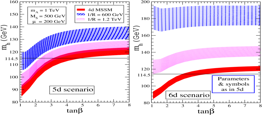
Figure 3.3: The dependence of ${\rm m}_{h}$ on $\tan\beta$ (zoomed for the low values) in 5d (left panel) and 6d (right panel) MSSM. The width of each band corresponds to the variation of $A_{t}$ and $A_{b}$ in the range $(0.8-1.2)M_{S}$.

As mentioned earlier, the current lower bound on ${\rm m}_{h}$ of 114.5 GeV excludes low values of $\tan\beta$ in the 4d MSSM. It is expected that in the extra-dimensional scenarios some of this excluded range of $\tan\beta$ will make it into the allowed zone. In Fig. 3.3, we have shown the variation of ${\rm m}_{h}$ with respect to $\tan\beta$ (for low values) to illustrate this effect. For the 5d case (left panel), $1/R$ of even 1.2 TeV eases the tension somewhat while for $1/R$ of 600 GeV the effect is very prominent. For 6d (right panel), the extra-dimensional contributions are further enhanced and the restriction on $\tan\beta$ is essentially entirely lifted. We should recall that $\tan\beta$ enters in the Higgs couplings to other particles and so the above result has significant bearing on collider searches of supersymmetry.

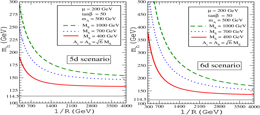
Figure 3.4: The dependence of ${\rm m}_{h}$ on $1/R$ for different choices of $M_{S}$ for 5d (left panel) and 6d (right panel) cases. The ratio $\sqrt{6}$ between $A_{t}(=A_{b})$ and $M_{S}$ maximises the trilinear contribution.

So far, we have exhibited results for a few choices of the compactification scale, $1/R$. Fig. 3.4 demonstrates how the KK-induced radiative correction depends on $1/R$ for the 5d (left panel) and 6d (right panel) scenarios. If the Higgs boson is detected at the LHC then using these figures one can gain a handle on $1/R$ dependent on the supersymmetry parameters like $M_{S}$. The decoupling behaviour as $1/R$ increases is in agreement with expectation.

We have also studied, in passing, the possibility that the soft supersymmetry breaking scale arises from compactification (e.g. through the Scherk-Schwarz mechanism [56]). Let us suppose $M_{S}=C/R$, where $C$ is an order one dimensionless constant. Since we are interested in weak scale supersymmetry breaking, we keep $1/R$ around a few hundred GeV to a TeV. In this region, the radiative correction roughly depends on $M_{S}$ and $R$ only through their product ($\equiv C$), and for a choice of $C\in[0.5-2.0]$, the upper limit on the lightest Higgs mass turns out to be in the range ${\rm m}_{h}\in(150-230)$ GeV (5d) and $(200-450)$ GeV (6d).

It may bear mentioning again that in these calculations we have retained the loop conntributions from the $t$ and $b$ quarks only. The other quarks and gauge bosons make negligible impact. Also, we have dealt only with real MSSM parameters and limited our studies up to one-loop KK contributions. We have not, therefore, included either the two-loop improvements of the 4d MSSM calculations or the numerical effects of the phases associated with complex MSSM parameters in our discussions (for a recent survey, see [59]).

3.5 Conclusions

One of the virtues for which supersymmetry stands out as a leading candidate of physics beyond the SM is that it sets an upper bound on the Higgs mass. The lightest neutral Higgs mass, ${\rm m}_{h}$, could at most be ${\rm m}_{Z}$ at the tree level, but is pushed further obeying a definite relation, obtained from quantum corrections, involving ${\rm m}_{h}$, ${\rm m}_{t}$ and the stop squark mass, ${\rm m}_{\tilde{t}}$. The sensitivity of this correction to ${\rm m}_{\tilde{t}}$ is only logarithmic. Consequently, a firm prediction results, namely, that ${\rm m}_{h}~{}\raisebox{-1.72218pt}{\hbox to0.0pt{$\sim$\hss}}\raisebox{1.72218pt}{$<$}~{}135$ GeV in MSSM for ${\rm m}_{\tilde{t}}~{}\raisebox{-1.72218pt}{\hbox to0.0pt{$\sim$\hss}}\raisebox{1.72218pt}{$<$}~{}{\cal{O}}$(1 TeV). This is regarded as a critical test of supersymmetry and is naturally high on the agenda of the upcoming LHC experiments. Here, we have probed how much this upper limit could be relaxed, should the MSSM be embedded in one ($S^{1}/Z_{2}$) or two ($T^{2}/Z_{4}$) extra dimensions. We highlight our main findings:

1. The KK towers of the top quark and stop squarks provide a positive contribution to ${\rm m}_{h}^{2}$ raising it by several tens of GeV. If we ignore left-right scalar mixing and assume moderate $\tan\beta\sim(5-10)$, then using Eq. (3.59) and summing over all the KK modes, we obtain $\Delta{\rm m}_{h}^{2}({\rm KK})\sim(60~{}{\rm GeV})^{2}\times(M_{S}R)^{2}$. This is a 5d result. Including the left-right scalar mixings, i.e., non-zero $\mu$ and trilinear parameters, somewhat enhances the magnitude of the correction (see Fig. 3.1). As in the case of 4d MSSM, here too the size of the correction is controlled by the large top Yukawa coupling.

2. If we consider a 6d theory with two extra dimensions compatcified on a chiral square, whose motivations have been mentioned earlier, the correction gets sizably enhanced (see Fig. 3.2), compared to 5d, due to a denser packing of KK states, which are now fixed by two independent KK numbers.

3. Non-observation of a Higgs boson weighing below 114.5 GeV disfavours low $\tan\beta$ in 4d MSSM. Some part of this region can be revived by extra-dimensional embedding (see Fig. 3.3).

4. The 4d MSSM relationship between the lightest neutral Higgs mass and the stop squark mass is extremely profound in the sense that its specific form does not depend on the supersymmetry breaking mechanism. If supersymmetry is embedded in extra dimension(s) and, with some cooperation from Nature, the KK states happen to be light enough to mark their imprints on the LHC data recorder, then the relationship between the stop mass and the Higgs mass alters in a numerically significant way (see Fig. 3.4).

Chapter 4 Low intermediate scales for leptogenesis in supersymmetric $SO(10)$ grand unified theories

4.1 Introduction

An area where the standard model based on the group $SU(3)_{C}\times SU(2)_{L}\times U(1)_{Y}\equiv{\cal G}_{std}$ merits improvement is the origin of parity violation. The most natural extension that addresses this issue is the left-right symmetric model in which the gauge group is enlarged to $SU(3)_{C}\times SU(2)_{L}\times SU(2)_{R}\times U(1)_{(B-L)}\equiv{\cal G}_{LR}$ [60]. Here, the left-handed fermions transform nontrivially under $SU(2)_{L}$ and are singlet under $SU(2)_{R}$, while it is the converse for the right-handed (RH) fermions. It is then possible to extend the definition of parity of the Lorentz group to all particles and ensure that the theory is invariant under the transformation of parity. Spontaneous breaking of the group $SU(2)_{R}$ would trigger violation of parity in the low energy theory. It is also possible to break the parity symmetry spontaneously by the vacuum expectation value of a gauge singlet scalar field which has odd parity [61]. In either case, parity violation at low energy originates from some spontaneous symmetry breaking at high energy.

Two experimental evidences for the existence of a theory beyond the standard model are the baryon asymmetry of the universe observed by the Wilkinson Microwave Anisotropy Probe (WMAP) [62] and the light neutrino mass as noted earlier. The see-saw mechanism can explain the light neutrino mass while the most viable mechanism to generate the matter antimatter asymmetry i.e baryon asymmetry is the baryogenesis via leptogenesis through the sphaleron processes. Actually, the tiny neutrino masses could be related with leptogenesis. In the SM $\nu$ is massless, but by the see-saw mechanism with inclusion of a right-handed neutrino or triplet Higgs scalar or both one can generate the tiny neutrino mass. The lepton number violating decays of the right-handed neutrino or the triplet Higgs scalar at some large scale, on the otherhand, can generate a lepton asymmetry, which is then converted into a baryon asymmetry of the universe.

As we discussed in sec. 1.6.2 the left-right symmetric extension of the standard model can emerge from a Grand Unified Theory based on the gauge group $SO(10)$. There are two broad classes of minimal $SO(10)$ models: those with only doublet Higgs scalars (Model I) and the conventional left-right symmetric model including triplet Higgs scalars (Model II). The main differences between Models I and II lie in the Higgs scalar that breaks the left-right symmetry and the generation of neutrino masses. Lepton number violation in these models arises from the Higgs scalars that break the $B-L$ symmetry and hence the left-right symmetry. The origin of leptogenesis is also different in these two models. There is a natural mechanism of resonant leptogenesis in Model I (see below) while Model II has other advantages.

In Model I there is an extra singlet fermion, $S$, that combines with the neutrinos and a new type of see-saw mechanism is operational [63]. There are several interesting features associated with this. The one relevant here is that the singlet fermions can be almost degenerate with the neutrinos, leading to resonant leptogenesis naturally in this scenario [64]. On the otherhand Model II is truly a renormalizable high scale SUSY SO(10) theory of fermion masses and mixings.

From an analysis of gauge coupling unification, we have determined the scale of left-right symmetry breaking, which is intimately related to a successful prediction of leptogenesis in these models. An apparent obstacle arises in the following form: either these models do not allow any intermediate mass scales or the intermediate left-right symmetry breaking scale comes out to be large ($\sim 10^{15}$ GeV). To implement leptogenesis, on the other hand, the left-right symmetry breaking scale has to be much lower. We exhibit several alternate possibilities which may provide a way out from this impasse.

The Majorana mass of right-handed neutrinos is given by $M_{N}\sim\tilde{f}v_{R}$, where $\tilde{f}$ is the Yukawa coupling and $v_{R}$ is the vev given to $\chi_{R}$, defined in sec. 1.6.2. The right-handed neutrino mass-scale controls leptogenesis as well as light neutrino masses and, in particular, a value around $10^{9}$ GeV or lower is favored by the ‘gravitino constraint’ discussed below. Since $\tilde{f}$ does not affect the experimentally measured charged fermion masses at low energies, one can assign any value to it, leaving the left-right symmetry breaking scale unrestricted. However, such a low RH neutrino mass is likely to give too large contributions to the left-handed neutrino masses through the see-saw mechanism, contradicting experimental observation. The main motivation of the see-saw mechanism was to avoid arbitrarily small Yukawa couplings, so we shall assume the value of $\tilde{f}$ to be of order unity .

While considering leptogenesis in the minimal supersymmetric $SO(10)$ GUTs, the potential problem [65] arising from the overclosure of the universe by gravitinos (and its adverse influence on the successful Big Bang Nucleosynthesis predictions) must be taken into account. This requires the reheating temperature, $T_{RH}$, to be less than $\sim 10^{8}$ GeV. Since leptogenesis takes place just below the scale of left-right symmetry breaking, $M_{R}>T_{RH}$ can make models inconsistent with the above or at least unnatural. However, Model I may still be consistent because it offers the alternative of resonant leptogenesis.

Using renormalization group (RG) equations, in the following sections we examine for both Models whether gauge coupling unification at all allows a low left-right symmetry breaking scale which would make successful leptogenesis viable. The simplicity of the minimal supersymmetric $SO(10)$ GUT allows several interesting predictions. With some standard assumptions it is possible to determine the mass scales involved in the symmetry breaking. Below, we shall show that one-loop renormalization group evolution leads to left-right symmetry breaking and unification scales,

$${M_{R}}^{0}\simeq 1.3\times 10^{16}~{}{\rm GeV},~{}~{}~{}~{}{M_{U}}^{0}\simeq 2.9\times 10^{16}~{}{\rm GeV}.$$ (4.1)

$M_{R}^{0}$ and $M_{U}^{0}$ are already very close. But, the situation worsens when two-loop RG contributions are included and we find that no intermediate scales are allowed at all below the unification scale. All this makes leptogenesis unnatural in this class of models. We suggest some possible remedies [67].

In this chapter we show how inclusion of GUT-threshold effects, gravitational corrections through $\rm{dim}.5$ operators, or presence of additional light fields near $M_{R}$, can lower the intermediate scale, bringing it even to the range of a few TeV in the doublet model. Thus, in this model, the gravitino constraint can be easily satisfied leading to successful resonant leptogenesis at low scales. In addition, the signatures of right-handed gauge bosons, ($W_{R}^{\pm}$, $Z_{R}$), and new Higgs scalars can be tested at the LHC and ILC. In the triplet model, on the other hand, even though the GUT threshold corrections are much larger, we derive a bound on the intermediate scale, $M_{R}>10^{9}$ GeV arising out of the requirement of perturbation theory to be valid, due to which the scale cannot be reduced further. With this lower bound on $M_{R}$ the triplet model emerges genuinely as a high scale supersymmetric theory for successful description of fermion masses and mixings.

The chapter is organised in the following manner. In sec. 4.1.1 we discuss renormalization group equations and origins of threshold and Planck scale effects. Discussing SUSY $SO(10)$ model and left-right symmetric breaking in sec. 4.1.2 and 4.2 respectively, we will show in sec. 4.3 how low intermediate scales are obtained in the doublet model and triplet model. The perturbative lower bound on $M_{R}$ is derived in sec. 4.4. After making brief remarks on fermion masses and light scalars in the SUSY $SO(10)$ model in sec. 4.5, we summarise the results and state our conclusions in sec. 4.6.

4.1.1 General formulation

We have already discussed the renormalisation group superficially for the standard model and supersymmetric standard model in sec. 1.6.3 and sec. 1.7.1 respectively. Let us first gather all the RGE with two loop contributions. We have also mentioned how these equations will change in the presence of some threshold correction or due to the Planck scale effects. The RG equations with one intermediate scale, $M_{R}$, between $M_{U}$ and $M_{Z}$ are:

$${1\over{\alpha_{i}}(M_{Z})} = {1\over\alpha_{i}(M_{R})}+{a_{i}\over 2\pi}\ln{M_{R}\over M_{Z}}+\Theta_{i}-\Delta_{i},$$ (4.2)

$${1\over\alpha_{i}(M_{R})} = {1\over\alpha_{i}(M_{U})}+{a^{\prime}_{i}\over 2\pi}\ln{M_{U}\over M_{R}}+\Theta^{\prime}_{i}-\Delta^{\prime}_{i}-\Delta_{i}^{(gr)},$$

where $i$ runs over the different gauge couplings. Let us clarify different notations used in the above two equations. In the R.H.S. of eqns. (4.2) and (LABEL:eqA.2), the second and third terms represent one- and two-loop contributions, respectively, with

$$\Theta_{i} = {1\over 4\pi}\sum_{j}B_{ij}\ln{\alpha_{j}(M_{R})\over\alpha_{j}(M_{Z})},$$

$$\Theta^{\prime}_{i} = {1\over 4\pi}\sum_{j}B^{\prime}_{ij}\ln{\alpha_{j}(M_{U})\over\alpha_{j}(M_{R})},$$

$$B_{ij} = {b_{ij}\over a_{j}},\,B^{\prime}_{ij}={b^{\prime}_{ij}\over a^{\prime}_{j}}.$$ (4.4)

The one- and two-loop coefficients ($a_{j},a^{\prime}_{j},b_{ij},b^{\prime}_{ij}$) for specific scenarios are given later. Between $M_{Z}$ and $M_{R}$ the indices $i,j\subset{\cal G}_{std}$ while above $M_{R}$ one has $i,j\subset{\cal G}_{LR}$.

The $\Delta_{i}$ include SUSY threshold effects and intermediate scale threshold effects at $M_{R}$,

$$\Delta_{i}=\Delta^{(S)}_{i}+\Delta^{(R)}_{i},$$

while $\Delta^{\prime}_{i}$ includes the same at the unification scale $M_{U}$. They are represented as [68, 69, 70, 71],

$$\Delta_{i}^{(S)} = \frac{1}{2\pi}\Sigma_{\alpha}b_{i}^{\alpha}\ln{{M^{\alpha}}\over M_{S}}\equiv\frac{b_{i}}{2\pi}\ln{{M_{i}}\over{M_{S}}},\;\;\;b_{i}=\Sigma_{\alpha}b_{i}^{\alpha},$$

$$\Delta_{i}^{(R)} = \frac{1}{2\pi}\Sigma_{\beta}{c}_{i}^{\beta}\ln{{M^{\beta}}\over M_{R}}\equiv\frac{b^{\prime}_{i}}{2\pi}\ln{{M_{i}}\over{M_{R}}},\;\;\;b^{\prime}_{i}=\Sigma_{\beta}{c}_{i}^{\beta},$$

$$\Delta^{\prime}_{i} = \frac{1}{2\pi}\Sigma_{\gamma}{d}_{i}^{\gamma}\ln{{M^{\gamma}}\over M_{U}}\equiv\frac{b^{\prime\prime}_{i}}{2\pi}\ln{{M_{i}}\over{M_{U}}},\;\;\;b^{\prime\prime}_{i}=\Sigma_{\gamma}{d}_{i}^{\gamma}.~{}~{}~{}~{}$$ (4.5)

Here the indices $\alpha,\beta$ and $\gamma$ signify the particle components of $SO(10)$ representations spread around the SUSY scale $M_{S}$, the $SU(2)_{R}\times U(1)_{B-L}$ breaking scale $M_{R}$, and the $SO(10)$ breaking scale $M_{U}$, respectively.

The definition of effective mass parameters at the SUSY scale $M_{S}$ through the first of eqns. (4.5) introduced by Carena, Pokorski and Wagner [68] has been generalised to study GUT-threshold effects by Langacker and Polonsky [70] in SUSY $SU(5)$ and in ref. [71] to study intermediate breaking in SUSY $SO(10)$. The effective mass parameters defined through these relations are not arbitrary. Logarithm of each of them is a well defined linear combination of logarithms of actual particle masses (heavy or superheavy) spread around the respective thresholds. Hence, in principle, it is possible to express them in terms of the parameters of the superpotential. The actual relationship would vary from model to model depending upon the type and number of representations used in driving the spontaneous symmetry breaking of SUSY $SO(10)$ to the low energy theory.

In the absence of unnatural mass spectra, the particles are expected to be a few times heavier or lighter than the associated threshold scale which would result in the effective mass parameters bearing a similar relationship to that scale.

The term $\Delta^{gr}_{i}$ represents the effect of $\rm{dim}.5$-operators which may be induced at the Planck scale as [72, 73],

$$\Delta_{i}^{(gr)} = -{{\epsilon}_{i}\over{\alpha}_{G}},i=BL,2L,2R,3C.$$ (4.6)

These operators modify the boundary condition at $M_{U}$ as ,

$$\alpha_{2L}(M_{U})(1+\epsilon_{2L})=\alpha_{2R}(M_{U})(1+\epsilon_{2R})=\alpha_{BL}(M_{U})(1+\epsilon_{BL})=\alpha_{3C}(M_{U})(1+\epsilon_{3C})=\alpha_{G}.$$

(4.7)

Here, $\alpha_{G}=g^{2}(M_{U})/{4\pi}$ is the GUT fine-structure constant. The impact of various contributions in eqns. (4.5) and (4.6) in lowering the intermediate scale in SUSY $SO(10)$ GUTs will be discussed in detail in subsequent sections.

Using eqns. (4.2) - (4.7) one obtains for the mass scales [71],

$$\ln{M_{R}\over M_{Z}} = {1\over(AB^{\prime}-A^{\prime}B)}[(AL_{S}-A^{\prime}L_{\Theta})+(A^{\prime}J_{2}-AK_{2})-{2\pi\over\lambda_{G}}(A\epsilon^{\prime\prime}-A^{\prime}\epsilon^{\prime})+(A^{\prime}J_{\Delta}-AK_{\Delta})],$$

$$\ln{M_{U}\over M_{Z}} = {1\over(AB^{\prime}-A^{\prime}B)}[(B^{\prime}L_{\Theta}-BL_{S})+(BK_{2}-B^{\prime}J_{2})-{2\pi\over\lambda_{G}}(B^{\prime}\epsilon^{\prime}-B\epsilon^{\prime\prime})+(BK_{\Delta}-B^{\prime}J_{\Delta})],$$

where

$$L_{S} = {2\pi\over\lambda(M_{Z})}\left(1-{8\over 3}{\lambda(M_{Z})\over\lambda_{S}(M_{Z})}\right),$$

$$L_{\Theta} = {2\pi\over\alpha(M_{Z})}\left(1-{8\over 3}\sin^{2}\Theta_{W}(M_{Z})\right),$$

$$A = a^{\prime}_{2R}+{2\over 3}a^{\prime}_{BL}-{5\over 3}a^{\prime}_{2L},$$

$$B = {5\over 3}(a_{Y}-a_{2L})-A,$$

$$A^{\prime} = \left(a^{\prime}_{2R}+{2\over 3}a^{\prime}_{BL}+a^{\prime}_{2L}-{8\over 3}a^{\prime}_{3C}\right),$$

$$B^{\prime} = {5\over 3}a_{Y}+a_{2L}-{8\over 3}a_{3C}-A^{\prime}.$$ (4.10)

$$J_{2} = 2\pi\left[\Theta^{\prime}_{2R}+{2\over 3}\Theta^{\prime}_{BL}-{5\over 3}\Theta^{\prime}_{2L}+{5\over 3}(\Theta_{Y}-\Theta_{2L})\right],$$

$$K_{2} = 2\pi\left[\Theta^{\prime}_{2R}+{2\over 3}\Theta^{\prime}_{BL}+\Theta^{\prime}_{2L}-{8\over 3}\Theta^{\prime}_{3C}\right.+\left.{5\over 3}\Theta_{Y}+\Theta_{2L}-{8\over 3}\Theta_{3C}\right],$$

$$\epsilon^{\prime} = \epsilon_{2R}+{2\over 3}\epsilon_{BL}-{5\over 3}\epsilon_{2L},$$

$$\epsilon^{\prime\prime} = \epsilon_{2L}+\epsilon_{2R}+{2\over 3}\epsilon_{BL}-{8\over 3}\epsilon_{3C},$$

$$J_{\Delta} = -2\pi\left[\Delta^{\prime}_{2R}+{2\over 3}\Delta^{\prime}_{BL}-{5\over 3}\Delta^{\prime}_{2L}+{5\over 3}(\Delta_{Y}-\Delta_{2L})\right],$$

$$K_{\Delta} = -2\pi\left[\Delta^{\prime}_{2R}+{2\over 3}\Delta^{\prime}_{BL}+\Delta^{\prime}_{2L}-{8\over 3}\Delta^{\prime}_{3C}\right.\left.+{5\over 3}\Delta_{Y}+\Delta_{2L}-{8\over 3}\Delta_{3C}\right].$$ (4.11)

4.1.2 The minimal SUSY $SO(10)$ models

In this subsection we apply the RG evolution detailed above to the specific minimal $SO(10)$ models keeping only the one- and two-loop contributions in eqns. (4.2) - (4.11).

The symmetry breaking proceeds through three steps. These are

• In the first step, the $SO(10)$ symmetry is broken at $M_{U}$ by the $vev$ of a ${\bf 210}$ multiplet. As noted earlier, it is chosen to be along the neutral component of $\{15,1,1\}$ under ${\cal G}_{PS}$ which is even under D-parity [61]. Thus, the gauge symmetry is broken to ${\cal G}_{LR}$ and, with unbroken D-parity, left-right discrete symmetry survives preserving $g_{2L}=g_{2R}$.

• In the second step, the breaking is different for the two models.

  1. In Model I (the doublet model), the $vev$ of the neutral component of ${\overline{\chi_{R}}}\subset{\bf\overline{16}}$ which transforms as $(1,1,2,-1)$ under ${\cal G}_{LR}$ breaks $SU(2)_{R}\times U(1)_{B-L}\to U(1)_{Y}$ at $M_{R}$. The left-handed doublets $\chi_{L}(1,2,1,-1)\oplus{\overline{\chi_{L}}}(1,2,1,1)$ and other components of $\chi_{R}(1,1,2,-1)\oplus{\overline{\chi_{R}}}(1,1,2,1)$ not absorbed by the RH gauge bosons remain light with masses around the intermediate scale $M_{R}$.

  2. In Model II (the triplet model) the $vev$ is assigned to the neutral component of a field $\overline{\Delta}_{R}\equiv$ (1,1,3,2) contained in a ${\bf\overline{126}}$. In this alternative, the left-handed triplets $\Delta_{L}(1,3,1,-2)\oplus{\overline{\Delta_{L}}}(1,3,1,2)$ contained in the ${\bf 126}$ and ${\bf\overline{126}}$ as well as other components of $\Delta_{R}(1,1,3,-2)\oplus{\overline{\Delta_{R}}}(1,1,3,2)$ not absorbed by the RH gauge bosons remain light and contribute to the gauge coupling evolution from $M_{R}$.

• Finally, the standard doublet Higgs contained in the bi-doublet $\phi(1,2,2,0)\subset{\bf 10}$ drives the symmetry breaking of ${\cal G}_{std}\to SU(3)_{C}\times U(1)_{em}$ at the electroweak scale. For simplicity, in the remainder of this section it is assumed that the supersymmetry scale, $M_{S}$, is the same as $M_{Z}$.

One major difficulty in obtaining the parity conserving ${\cal G}_{LR}$ intermediate symmetry originates from the mass spectra predictions in the triplet model with certain colored Higgs components of $G_{PS}$ multiplets in $\{15,3,1\}+\{15,1,3\}\subset{\bf 210}$ being at the $M_{R}$ scale [74]. We note that a similar difficulty also arises in the minimal doublet model unless these states are made superheavy through the presence of additional $SO(10)$ Higgs representations or non-renormalizable terms in the superpotential as discussed in sec. 4.5. Assuming that these additional scalars are made superheavy, our RG analysis applies with the minimal particle content between $M_{Z}$ to $M_{U}$ as described above.

For Model I, the MSSM one- and two-loop beta-function coefficients below the scale $(M_{R})$ are given by,

$$\left(\begin{array}[]{c}a_{Y}\\ a_{2L}\\ a_{3C}\end{array}\right)=\left(\begin{array}[]{c}{33\over 5}\\ 1\\ -3\end{array}\right),~{}~{}~{}~{}b_{ij}=\left(\begin{array}[]{ccc}{199\over 25}&{27\over 5}&{88\over 5}\\ {9\over 5}&25&24\\ {11\over 5}&9&14\end{array}\right),i,j\subset{\cal G}_{std}.$$ (4.21)

Above $M_{R}$ till $M_{U}$ the beta-function coefficients are

$$\left(\begin{array}[]{c}a^{\prime}_{BL}\\ a^{\prime}_{2L}\\ a^{\prime}_{2R}\\ a^{\prime}_{3C}\end{array}\right)=\left(\begin{array}[]{c}9\\ 2\\ 2\\ -3\end{array}\right),~{}~{}b^{\prime}_{ij}=\left(\begin{array}[]{cccc}{23/2}&{27/2}&{27/2}&{8}\\ {9/2}&{32}&{3}&{24}\\ {9/2}&{3}&{32}&{24}\\ {1}&{9}&{9}&{14}\end{array}\right),i,j\subset{\cal G}_{LR}.$$ (4.34)

Using $\alpha_{S}(M_{Z})=0.1187$, $\alpha(M_{Z})=1/127.9$, and $\sin^{2}\Theta_{W}=0.2312$, the one-loop solutions yield

$$M_{R}^{0}=1.3\times 10^{16}~{}{\rm GeV~{}~{}~{}~{}~{},}~{}~{}~{}~{}~{}M_{U}^{0}=2.9\times 10^{16}~{}{\rm GeV}.~{}~{}~{}~{}~{}$$ (4.35)

The GUT fine structure constant is $\alpha_{G}\simeq 1/24.25$. When two-loop contributions are included then, as noted earlier, no intermediate symmetry breaking scale is permitted at all.

For Model II, below $M_{R}$ the one- and two-loop beta function coefficients are still given by eq. (4.21) while between $M_{R}$ and $M_{U}$ we have

$$\left(\begin{array}[]{c}a^{\prime}_{BL}\\ a^{\prime}_{2L}\\ a^{\prime}_{2R}\\ a^{\prime}_{3C}\end{array}\right)=\left(\begin{array}[]{c}24\\ 5\\ 5\\ -3\end{array}\right),~{}~{}b^{\prime}_{ij}=\left(\begin{array}[]{cccc}{115}&{81}&{81}&{8}\\ {27}&{73}&{3}&{24}\\ {27}&{3}&{73}&{24}\\ {1}&{9}&{9}&{14}\end{array}\right),i,j\subset{\cal G}_{LR}.$$ (4.48)

In this case, the one-loop evolution results in

$$M_{R}^{0}=7.9\times 10^{15}~{}{\rm GeV~{},}~{}~{}~{}~{}~{}M_{U}^{0}=1.9\times 10^{16}~{}{\rm GeV},$$ (4.49)

with the GUT fine structure constant $\alpha_{G}\simeq 1/24.00$. As in Model I, inclusion of two-loop effects disallows any intermediate scale.

We shall now turn to the implication of this high intermediate left-right symmetry breaking in the context of neutrino masses and leptogenesis. Then we will exhibit ways by which the difficulties can be evaded.

4.2 Low scale left-right symmetry breaking

As noted in the previous section, in the minimal supersymmetric $SO(10)$ models the left-right symmetry breaking intermediate scale cannot be lower than $10^{15}$ GeV. We shall briefly illustrate the application of Model II for successful explanation of fermion masses and mixings with such a high value of $M_{R}$.

In Model II, the left-right symmetry is broken by the $vev$ of the right-handed triplet Higgs scalar $\bar{\Delta}_{R}\equiv(1,1,3,2)\subset{\bf\overline{126}}$. The left-handed triplet Higgs scalar $\bar{\Delta}_{L}\equiv(1,3,1,2)$ required by left-right symmetry is also present in ${\bf\overline{126}}$. The bi-doublet Higgs that breaks the electroweak symmetry and the Higgs that breaks the $SO(10)$ group are $\phi\equiv(1,2,2,0)\subset{\bf 10}$ and $\Phi\equiv(1,1,1,0)\subset{\bf 210}$. Since we are concerned with neutrino masses and leptogenesis, consider the Yukawa interactions of the left- and right-handed leptons:

$$\psi_{L}\equiv\left(\begin{array}[]{c}\nu\\ e\end{array}\right)_{L}\equiv(1,2,1,-1)\subset{\bf 16},$$ (4.52)

$$\psi_{R}\equiv\left(\begin{array}[]{c}\nu\\ e\end{array}\right)_{R}\equiv(1,1,2,-1)\subset{\bf 16}.$$ (4.55)

The relevant Yukawa couplings are given by

$${\cal L}_{Y}=f\overline{\psi}_{L}\psi_{R}\phi+\tilde{f}\overline{\psi^{c}_{L}}\psi_{L}\bar{\Delta}_{L}+\tilde{f}\overline{\psi^{c}_{R}}\psi_{R}\bar{\Delta}_{R}.$$ (4.56)

In eqn.(4.56), the field $\psi^{c}$ is the charge conjugation of the field $\psi$ defined as

$$\psi^{c}=C\psi^{*},$$ (4.57)

where, $C=i\gamma_{2}\gamma_{0}$ in the Dirac-Pauli representation. Then the neutrino mass matrix can be written as

$$M_{\nu}=\left(\begin{array}[]{cc}\nu&\nu^{c}\end{array}\right)_{L}\left(\begin{array}[]{cc}m_{L}&m_{D}\\ m_{D}&m_{R}\end{array}\right)\left(\begin{array}[]{c}\nu\\ \nu^{c}\end{array}\right)_{L},$$ (4.63)

where, $m_{L}=\tilde{f}\langle{\bar{\Delta}_{L}}\rangle;~{}~{}m_{R}=\tilde{f}\langle{\bar{\Delta}_{R}}\rangle$ and $m_{D}=f\langle\phi\rangle$. Generation indices have been suppressed. The right-handed neutrinos then remain massive, while the left-handed neutrino masses are see-saw suppressed

$$m_{N} = m_{R},$$

$$m_{\nu} = m_{L}-{m_{D}^{2}\over m_{R}}.$$ (4.64)

The first term $m_{L}=\tilde{f}v_{L}$ is also naturally small, since

$$v_{L}=\langle\bar{\Delta}_{L}\rangle=\kappa v^{2}/v_{R}.$$

With supersymmetry in $SO(10)$, $\kappa$ is model dependent and some fine-tuning of this parameter is needed in the triplet model to achieve type II see-saw dominance, successful prediction of large neutrino mixings and parameterization of all fermion masses and mixings including CP-violation [74, 75, 76, 77]. With asymptotic parity invariance in the high scale theory, the gravitino constraint is often ignored in the triplet model [66]. Moreover, the observed smallness of neutrino masses may work against bringing the left-right symmetry breaking scale closer to $10^{9}$ – $10^{10}$ GeV in the triplet model.

In Model I, we will explore an alternative approach where, without fine-tuning of the Yukawa couplings of the see-saw formula, the left-right symmetry breaking scale can be sufficiently lowered to meet the requirements of resonant leptogenesis while satisfying the gravitino constraint and maintaining consistency with experimentally observed small values of neutrino masses.

As discussed in subsequent sections, both the $SO(10)$ representations $\bf{210}$ and $\bf{54}$ are necessary to break $SO(10)\to{\cal{G}}_{LR}$ in Model I as well as in Model II, to prevent certain undesirable scalar components of $\bf{210}$ being lighter than the GUT scale and upsetting successful gauge coupling unification.

In Model I, neutrino masses arise from the Yukawa Lagrangian:

$${\cal L}_{Y}=f\overline{\psi}_{L}\psi_{R}\phi+y\left(\overline{\psi}_{L}S\chi_{L}+\overline{\psi}_{R}S\chi_{R}\right)+MS^{T}S+H.c.$$ (4.65)

where ${\chi_{L}}(1,2,1,-1)$ and ${\chi_{R}}(1,1,2,-1)$ are in the 16 dimensional Higgs representation, $\phi$ is in a 10, and $S$ stands for $SO(10)$ singlets, of which there are three.

The left-handed neutrinos $\nu_{L}$ and the right-handed neutrinos $N=\nu_{R}$ now mix with the new singlet fermions $S$ through the mass matrix:

$$M_{\nu}=\left(\begin{array}[]{ccc}\nu&N^{c}&S\end{array}\right)_{L}\left(\begin{array}[]{ccc}0&m_{D}&yv_{L}\\ m_{D}&0&yv_{R}\\ yv_{L}&yv_{R}&M\end{array}\right)\left(\begin{array}[]{c}\nu\\ N^{c}\\ S\end{array}\right)_{L}.$$ (4.73)

Here the Dirac neutrino mass, $m_{D}$, the Yukawa coupling, $y$, and the singlet fermion mass, $M$, are $3\times 3$ matrices. Light left-handed neutrino masses matching the experimental data arise from this mass matrix through the double see-saw and type III see-saw mechanisms, as has been widely discussed in the literature [63, 78, 79]. The model gives desired values of neutrino masses even for low left-right symmetry breaking scales without fine-tuning of the Yukawa couplings.

4.3 Different techinques to achieve low intermediate scale

We have advanced the following possibilities which may lead to left-right symmetry breaking at energies much lower than in the the minimal models:

• Threshold Correction: In the conventional analysis, one assumes that different states within a GUT multiplet have the same mass. This is not exact and small splittings usually do arise. The threshold effect due to a superheavy mass state contributes to a small log at one-loop level; but in $SO(10)$ where big-sized representations like ${\bf 210}$ or ${\bf 126+\overline{126}}$ or both are used, the one-loop contributions by a large number of superheavy components lead to substantial modification of the gauge couplings near the GUT scale. Both the doublet and the triplet $SO(10)$ models belong to this category. Thus threshold effects in each of them might significantly change the allowed values of $M_{R}$ obtained from the unification constraint.

• Non-renormalizable interactions at the Planck scale: Since the unification scale is close to the scale of quantum gravity, there may arise gauge invariant but non-renormalizable interaction terms in the Lagrangian suppressed by inverse powers of the Planck scale or a string compactification scale. They affect the gauge coupling values at the GUT scale and change the predictions of the minimal models.

• Additional light fields: If there are any additional light multiplets in the theory, they can modify the evolution of the gauge couplings and can allow a lowered $M_{R}$.

In the following, we have given details of these possibilities and shown that with each of them it is possible to get lower scale left-right symmetry breaking which in some cases could even be low enough to be within striking range of the LHC/ILC.

4.3.1 Threshold effects

Conventionally, superheavy GUT multiplets are considered to be degenerate. In general, however, the members of a representation could possess somewhat different masses spread around the GUT scale giving rise to sizable modifications of the gauge coupling constant predictions and the mass scales via threshold effects [80, 81, 82]. In the absence of precise information of the actual values of these masses, one may assume that all the components of a particular submultiplet are degenerate, but different submultiplets have masses that are spread closely around the scale of symmetry breaking [81]. In an alternate method, one introduces a set of effective mass parameters to capture the threshold effects [68]. Such an approach has been used at the SUSY $SU(5)$ scale to examine uncertainties in the GUT model predictions [70]. This procedure is extended here to the ${\cal G}_{LR}$ symmetry breaking scale in the form of eq. (4.5) [71].

Below, we examine to what extent threshold corrections could lower the scale of left-right symmetry breaking. We assume all superheavy gauge bosons to possess degenerate masses identical to the unification scale $M_{U}$.

Model I: For the particle content of Model I, from eq. (4.10) one obtains

$$A=B=14/3,~{}A^{\prime}=18,~{}B^{\prime}=2,~{}AB^{\prime}-A^{\prime}B=-224/3,\\$$ (4.74)

Using these, one has from eqns. (LABEL:eqA.5), (LABEL:eqA.6), and (4.11) the following expressions for threshold corrections on $M_{R}$ and $M_{U}$:

$$\Delta\ln{M_{R}\over M_{Z}} = {\pi\over 14}\left[{10\over 3}\Delta^{\prime}_{BL}-8\Delta^{\prime}_{2L}+{14\over 3}\Delta^{\prime}_{3C}+{25\over 3}\Delta_{Y}-13\Delta_{2L}+{14\over 3}\Delta_{3C}\right],$$

$$\Delta\ln{M_{U}\over M_{Z}} = {\pi\over 28}\left[{4\over 3}\Delta^{\prime}_{BL}+8\Delta^{\prime}_{2L}-{28\over 3}\Delta^{\prime}_{3C}+{10\over 3}\Delta_{Y}+6\Delta_{2L}-{28\over 3}\Delta_{3C}\right].$$ (4.75)

The quantities appearing on the RHS of eq. (4.75) are readily calculated using eq. (4.5), given the superheavy components of $\bf{210}\oplus{16}\oplus{\overline{16}}\oplus{10}$. In this manner one gets [71],

$$b^{\prime\prime}_{2L}=b^{\prime\prime}_{2R}=53,~{}~{}b^{\prime\prime}_{3C}=56,~{}~{}b^{\prime\prime}_{BL}=50,\\$$ (4.76)

leading to

$$\Delta\ln{M_{R}\over M_{Z}} = {1\over 7}\left[{125\over 3}\ln{M_{1}\over M_{U}}-106\ln{M_{2}\over M_{U}}+{196\over 3}\ln{M_{3}\over M_{U}}\right],$$

$$\Delta\ln{M_{U}\over M_{Z}} = {1\over 7}\left[{25\over 3}\ln{M_{1}\over M_{U}}+53\ln{M_{2}\over M_{U}}-{196\over 3}\ln{M_{3}\over M_{U}}\right].$$ (4.77)

The pair of equations in (4.77) provide enough room to find solutions which will lead to a significant lowering of the scale $M_{R}$ while keeping $M_{U}$ within the Planck scale .

As an illustration, one can consider a one parameter solution satisfying:

$${M_{U}\over M_{1}}={M_{U}\over M_{3}}={M_{2}\over M_{U}}=\eta~{}.$$ (4.78)

One finds from eq. (4.77)

$$\Delta\ln{M_{R}\over M_{Z}}=-30.42\ln\eta,\;\;\;\Delta\ln{M_{U}\over M_{Z}}=15.71\ln\eta~{}.$$ (4.79)

Note that, in the absence of threshold corrections, at the two-loop level $\ln{M_{U}^{0}\over M_{Z}}=33.178$ and $\ln{M_{R}^{0}\over M_{Z}}=32.916$. To ensure that $M_{U}\leq M_{Pl}=1.2\times 10^{19}$ GeV one must satisfy $\left(\Delta\ln{M_{U}\over M_{Z}}\right)\leq 6.24$. Thus, from eq. (4.79) $\eta\leq 1.48$ leading to $\left(\Delta\ln{M_{R}\over M_{Z}}\right)\geq-12.07$ implying

$$M_{R}\geq 1.0\times 10^{11}~{}~{}{\rm{GeV}},~{}~{}M_{U}\leq 1.2\times 10^{19}~{}~{}{\rm{GeV}}.$$ (4.80)

$M_{R}$	$M_{U}$	${M_{1}\over M_{U}}$	${M_{2}\over M_{U}}$	${M_{3}\over M_{U}}$	${\alpha_{G}^{-1}}$
(GeV)	(GeV)
$10^{11}$	$1.2\times 10^{19}$	${(1.48)}^{-1}$	1.48	${(1.48)}^{-1}$	23.7
$10^{9}$	$10^{18}$	0.272	1.770	0.831	23.7
$10^{7}$	$10^{18}$	0.158	1.950	0.832	23.7
$10^{7}$	$5\times 10^{16}$	0.151	2.750	1.524	27.7
$10^{5}$	$5\times 10^{18}$	0.180	3.30	1.076	26.7
$10^{3}$	$10^{19}$	0.154	4.760	1.301	28.7

Table 4.1: Examples of low intermediate scale, $M_{R}$, coupling constant unification solutions triggered by GUT-scale threshold effects in Model I (the doublet model).

This simple example implies that with one parameter $\eta$, $M_{R}$ lower than that given in eq. (4.80) corresponds to unification scales higher than the Planck mass. Even this bound on $M_{R}$ can be further lowered by one order when smaller threshold effects from lower scales [69, 83] are included leading to $M_{R}\simeq 10^{10}$ GeV with near Planck scale grand unification in the minimal doublet model. In principle, there are three distinct mass scales $M_{i},i=1,2,3,$ that enter in the threshold corrections, see eq. (4.77), and there is much more flexibility to further lower $M_{R}$. We return to such solutions later.

It is interesting to examine how gauge coupling constants are matched by threshold corrections to reach their common unification value in spite of such substantial changes in both the mass scales. Using eq. (4.5) and eq. (4.76), for $\eta=1.48$ the GUT-threshold corrections for individual couplings are [71]

$$\Delta^{\prime}_{BL}=-{25\over\pi}\ln\eta=-3.16,\;\;\Delta^{\prime}_{2L}={53\over 2\pi}\ln\eta=3.35,\;\;\Delta^{\prime}_{3C}=-{28\over\pi}\ln\eta=-3.54.$$ (4.81)

The gauge couplings extrapolated from $M_{Z}$ to $M_{R}=10^{11}$ GeV are,

$$\alpha_{BL}^{-1}(M_{R})=53.4,~{}~{}\alpha_{2L}^{-1}(M_{R})=26.3,~{}~{}~{}\alpha_{3C}^{-1}(M_{R})=18.4.$$ (4.82)

With GUT-threshold effects, the one loop-evolution of the coupling constants from $M_{R}$ to the new value of $M_{U}$,

$${1\over\alpha_{i}(M_{U})} = {1\over\alpha_{i}(M_{R})}-{a^{\prime}_{i}\over 2\pi}\ln{M_{U}\over M_{R}}+\Delta^{\prime}_{i},~{}~{}~{}~{}~{}~{}i=2L,BL,3C.$$ (4.83)

Then using eq. (4.77) - eq. (4.82) in eq. (4.83),

$${1\over\alpha_{BL}(M_{U})}=23.1,\;\;\;{1\over\alpha_{2L}(M_{U})}=23.5,\;\;\;{1\over\alpha_{3C}(M_{U})}=23.7.$$ (4.84)

The one parameter solution has the virtue of simplicity. However, as noted earlier, in eq. (4.77) – see also eq. (4.5) – three distinct mass scales $M_{i},i=1,2,3,$ are, in general, required to capture the effect of the threshold corrections at the unification scale. Table 4.1 depicts a whole set of such solutions. For every solution, the effective mass splittings are within a tolerable range and the unification scale has been increased by the threshold corrections. The value of the unified gauge coupling is also shown.

Model II: The threshold effect analysis for Model II (the triplet model) can be carried out along the same lines as in Model I. Thus, from eq. (4.10) one finds:

$$A=38/3,~{}~{}~{}B=-10/3,$$

$$~{}A^{\prime}=34,~{}~{}~{}~{}B^{\prime}=-14,~{}~{}~{}~{}AB^{\prime}-A^{\prime}B = -64.$$ (4.85)

In place of eq. (4.75) one now has

$$\Delta\ln{M_{R}\over M_{Z}} = {\pi\over 2}\left[{8\over 9}\Delta^{\prime}_{BL}-3\Delta^{\prime}_{2L}+{19\over 9}\Delta^{\prime}_{3C}\right],$$

$$\Delta\ln{M_{U}\over M_{Z}} = {\pi\over 2}\left[{4\over 9}\Delta^{\prime}_{BL}-\Delta^{\prime}_{2L}+{5\over 9}\Delta^{\prime}_{3C}\right].$$ (4.86)

The one-loop beta-function coefficients from Model II required for an evaluation of the RHS are:

$$b^{\prime\prime}_{2L}=b^{\prime\prime}_{2R}=116,~{}~{}b^{\prime\prime}_{3C}=122,~{}~{}b^{\prime\prime}_{BL}=101.\\$$ (4.87)

Thus, from the superheavy components of $\bf{210}\oplus{126}\oplus{\overline{126}}\oplus{10}$ one gets [71]:

$$\Delta\ln{M_{R}\over M_{Z}} = \left[{202\over 9}\ln{M_{1}\over M_{U}}-{87}\ln{M_{2}\over M_{U}}+{1159\over 18}\ln{M_{3}\over M_{U}}\right],$$

$$\Delta\ln{M_{U}\over M_{Z}} = \left[{101\over 9}\ln{M_{1}\over M_{U}}-{29}\ln{M_{2}\over M_{U}}+{305\over 18}\ln{M_{3}\over M_{U}}\right].~{}~{}~{}~{}~{}~{}$$ (4.88)

Eqns. (4.88) depend, as in the case of Model I, on the three mass scales $M_{i},i=1,2,3$ which can be chosen appropriately to ensure a solution with a low intermediate scale $M_{R}$. A few typical examples are presented in Table 4.2. It is noteworthy that the gauge coupling at unification is larger for these solutions than for the ones in Table 4.1.

$M_{R}$	$M_{U}$	${M_{1}\over M_{U}}$	${M_{2}\over M_{U}}$	${M_{3}\over M_{U}}$	${\alpha_{G}^{-1}}$
(GeV)	(GeV)
$5\times 10^{9}$	$1.58\times 10^{16}$	2.204	1.200	0.659	15.0
$10^{10}$	$1.58\times 10^{16}$	2.065	1.160	0.659	15.0
$10^{11}$	$1.58\times 10^{16}$	1.661	1.050	0.656	15.0

Table 4.2: Examples of low intermediate scale, $M_{R}$, coupling constant unification solutions triggered by GUT-scale threshold effects in Model II (the triplet model).

Before moving on, let us remark that in many of the threshold effect driven solutions in Model I the unification scale is pushed to higher values. It is well known that suppression of Higgsino mediated supersymmetric proton decay modes like $p\to K^{+}{\overline{\nu}}$, $p\to K^{0}{\mu}^{+}$ etc. is a generic problem in minimal SUSY GUTs and the amplitudes are proportional to $M_{U}^{-2}$. The higher unification scales help to evade this problem in a natural and effective fashion with a suppression factor $({M_{U}^{0}\over M_{U}})^{2}=10^{-2}-10^{-4}$.

4.3.2 Planck scale effects

Since the GUT scale is close to the Planck mass, it is possible that gravity induced non-renormalizable terms could change the usual field theoretic predictions of gauge coupling unification. These interactions are suppressed by inverse powers of the Planck mass. For example, consider the gauge invariant Lagrangian consisting of the $\rm{dim}.5$ non-renormalizable operators (NRO),

$${\cal L}_{NRO} = -{\eta_{1}\over 2M_{G}}Tr\left(F_{\mu\nu}\Phi_{210}F^{\mu\nu}\right)-{\eta_{2}\over 2M_{G}}Tr\left(F_{\mu\nu}\Phi_{54}F^{\mu\nu}\right).$$ (4.89)

The effective gauge coupling constants at the unification point get changed due to these non-renormalizable terms. In particular, these interactions determine the parameters in eq. (4.7) and one finds [72, 73],

$$\epsilon_{2L} = \epsilon_{2R}=-{3\over 2}\epsilon_{2},~{}\epsilon_{3C}=\epsilon_{2}-\epsilon_{1},~{}~{}\epsilon_{BL}=2\epsilon_{1}+\epsilon_{2},$$

$$\epsilon^{\prime} = {4\over 3}\epsilon_{1}+{5\over 3}\epsilon_{2},~{}~{}\epsilon^{\prime\prime}=4\epsilon_{1}-5\epsilon_{2},$$

where

$$\epsilon_{1}={{3\eta_{1}}\over 4}{M_{U}\over M_{G}}\left[{1\over{4\pi\alpha_{G}}}\right]^{1\over 2},\;\;\;\epsilon_{2}={{3\eta_{2}}\over 4}{M_{U}\over M_{G}}\left[{1\over{15\pi\alpha_{G}}}\right]^{1\over 2},$$ (4.90)

leading to the following analytic expressions for the corrections on the mass scales,

$$\left(\Delta\ln{M_{R}\over M_{Z}}\right)_{gr} = {2\pi(A^{\prime}\epsilon^{\prime}-A\epsilon^{\prime\prime})\over\alpha_{G}(AB^{\prime}-A^{\prime}B)},=-{\pi\over{7\alpha_{G}}}\left[\epsilon_{1}+10\epsilon_{2}\right],$$

$$\left(\Delta\ln{M_{U}\over M_{Z}}\right)_{gr} = {2\pi(B\epsilon^{\prime\prime}-B^{\prime}\epsilon^{\prime})\over\alpha_{G}(AB^{\prime}-A^{\prime}B)}={\pi\over{7\alpha_{G}}}\left[5\epsilon_{2}-3\epsilon_{1}\right].~{}~{}~{}~{}~{}~{}~{}~{}$$ (4.91)

While the change in the mass scales are governed by the above relations the individual coupling constants near the GUT scale change as,

$$\Delta_{2L}^{\rm{(gr)}}={3\epsilon_{2}\over 2\alpha_{G}},\;\;\;\Delta_{BL}^{\rm{(gr)}}=-{\left(2\epsilon_{1}+\epsilon_{2}\right)\over\alpha_{G}},\;\;\;\Delta_{3C}^{\rm{(gr)}}={\left(\epsilon_{1}-\epsilon_{2}\right)\over\alpha_{G}}.$$ (4.92)

Using the most natural scale for the two NRO’s as the Planck mass, $M_{G}=1.2\times 10^{19}$ GeV, and eq. (4.90) - eq. (4.92) we searched for gravity corrected solutions for low intermediate mass scale and high GUT scale with the constraint $|\eta_{1,2}|\simeq O(1)$.

$M_{R}$	$M_{U}$	$\eta_{1}$	$\eta_{2}$	${\alpha_{G}^{-1}}$
(GeV)	(GeV)
$10^{9}$	$3.16\times 10^{18}$	0.305	0.96	25.00
$10^{7}$	$3.16\times 10^{18}$	0.494	1.16	25.64
$10^{6}$	$8\times 10^{17}$	2.728	4.77	25.32
$10^{5}$	$3.16\times 10^{18}$	0.671	1.34	25.32

Table 4.3: Sample coupling constant unification solutions with low intermediate scales, $M_{R}$, obtained for Model I (the doublet model) through Planck scale induced interactions parameterized by $\eta_{1}$ and $\eta_{2}$ (see text).

For example with $\epsilon_{1}=0.15$, $\epsilon_{2}=0.174$, $M_{G}=M_{Pl.}$ we have $M_{R}=10^{7}$ GeV and $M_{U}=10^{18.4}$ GeV, corresponding to $\eta_{1}=0.494$ and $\eta_{2}=1.160$. The corrections to the coupling constants are obtained through $\Delta_{BL}^{\rm{(gr)}}=-11.47$, $\Delta_{2L}^{\rm{(gr)}}=6.52$, and $\Delta_{3C}^{\rm{(gr)}}=0.6$ . When these are added to one-loop extrapolated values from $M_{Z}$ to $M_{U}~{}(\equiv 10^{18.4}$ GeV), the three coupling constants match consistently with their common value $\alpha_{G}^{-1}\simeq 25$. All solutions with high unification scales require $|\eta_{1,2}|\simeq O(1)$ as shown in Table 4.3. Thus, $\rm{dim.}5$ operators are capable of lowering the left-right symmetry breaking scale to $M_{R}=10^{5}-10^{9}$ GeV, making Model I consistent with large neutrino mixing and leptogenesis when the minimal doublet model is supplemented by the addition of a ${\bf 54}$.

We find that high values of $M_{U}\simeq 10^{18}$ GeV require smaller $\eta_{1,2}\simeq O(1)$ while a lower $M_{U}\simeq 10^{16}$ GeV requires unnaturally larger values of the parameters. The preferred solutions with naturally large values of $M_{U}$ exhibit the virtue of suppression of Higgsino mediated proton decay by factors $({M_{U}^{0}\over M_{U}})^{2}=10^{-3}-10^{-4}$.

We now extend the triplet model by the addition of a Higgs representation 54 and including the effects of the two non-renormalizable operators of eq. (4.89). The changes in the mass scales are given by

$$\left(\Delta\ln{M_{R}\over M_{Z}}\right)_{gr} = -{\pi\over{12\alpha_{G}}}\left[-2\epsilon_{1}+45\epsilon_{2}\right],$$

$$\left(\Delta\ln{M_{U}\over M_{Z}}\right)_{gr} = -{\pi\over{12\alpha_{G}}}\left[2\epsilon_{1}+15\epsilon_{2}\right].$$ (4.93)

Unlike for the doublet model, we find that gravitational corrections alone do not succeed in substantially reducing the $M_{R}$ scale. This behaviour of the triplet model can be understood in terms of the larger Higgs representations – 126 and ${\bf\overline{126}}$ – involved and the consequent tension with perturbativity (see Sec.4.4).

4.3.3 Doublet model with additional light multiplets

The third and final alternative that we discuss for obtaining a low intermediate scale in Model I is through additional light chiral submultiplets. We find that if there are appropriate light states in the particle spectrum then the unification of gauge couplings is consistent with a significant lowering of $M_{R}$.

In earlier work attempts have been made to obtain intermediate scales much lower than the GUT scale by spontaneous breaking of SUSY $SO(10)$ in the first step and the gauge group ${\cal G}_{LR}$ in the second step with or without [84] left-right discrete symmetry. The crucial point of this chapter is that we require the left-right symmetric gauge group with $g_{2L}=g_{2R}$ to survive to low intermediate scales in order to evade the gravitino problem and at the same time obtain low mass $W_{R}^{\pm}$ gauge bosons to possibly even provide testable signals at collider energies in the near future.

We present below two models which meet these requirements. The models are identical up till the scale $M_{R}$ and consist of the MSSM particles. They differ in the number and type of additional chiral multiplets which contribute in the range $M_{R}$ to $M_{U}$. In this subsection, we choose to distinguish between the SUSY scale, $M_{S}$ (which is chosen at 1 TeV), and $M_{Z}$. The RG evolution of the couplings from $M_{Z}$ to $M_{S}$ is governed by the one- and two-loop coefficients:

$$\left(\begin{array}[]{c}a_{Y}\\ a_{2L}\\ a_{3C}\end{array}\right)=\left(\begin{array}[]{c}{21\over 5}\\ -3\\ -7\end{array}\right),~{}~{}b_{ij}=\left(\begin{array}[]{ccc}{104\over 25}&{18\over 5}&{44\over 5}\\ {6\over 5}&8&12\\ {11\over 10}&{9\over 2}&-26\end{array}\right),\,i,j\subset{\cal G}_{std},$$ (4.103)

while from $M_{S}$ to the scale $M_{R}$ eq. (4.21) is applicable. In eq.(4.103) the beta-function coefficients have been derived assuming two light doublets in the nonSUSY model below $M_{S}$ which emerges naturally from the MSSM existing above $M_{S}$.

Model A: In addition to the MSSM particles, we assume that supermultiplets with the following gauge quantum numbers are light with masses at the $M_{R}$ scale:

$$\sigma(3,1,1,4/3)\oplus{\overline{\sigma}}(\overline{3},1,1,-4/3) \subset {\bf 45,210},$$

$$\eta(1,1,1,2)\oplus{\overline{\eta}}(1,1,1,-2) \subset {\bf 120}.$$ (4.104)

The one- and two-loop coefficients including these fields are,

$$\left(\begin{array}[]{c}a^{\prime}_{BL}\\ a^{\prime}_{2L}\\ a^{\prime}_{2R}\\ a^{\prime}_{3C}\end{array}\right)=\left(\begin{array}[]{c}16\\ 2\\ 2\\ -2\end{array}\right),$$ (4.113)

$$b^{\prime}_{ij}=\left(\begin{array}[]{cccc}{241/6}&{27/2}&{27/2}&{88/3}\\ {9/2}&{32}&{3}&{24}\\ {9/2}&{3}&{32}&{24}\\ {11/3}&{9}&{9}&{76/3}\end{array}\right),\,i,j=BL,2L,2R,3C.$$ (4.118)

At two-loop level the evolution of gauge couplings and their unification have been shown in Fig. 4.1 for $M_{R}=10^{4}$ GeV. Some sample solutions to the RGEs for gauge couplings with allowed values of $M_{R}$, $M_{U}$ and the GUT fine structure constant ($\alpha_{G}$) are presented in Table 4.4. We find that with the grand unification scale $M_{U}=2\times 10^{16}$ GeV, an intermediate scale in the range of $M_{R}=5$ TeV - $10^{10}$ GeV is possible in this model with excellent unification of the gauge couplings. In spite of the presence of additional fields, the gauge couplings at the GUT scale remain perturbative in a manner similar to the minimal GUT with $\alpha_{G}^{-1}=22.22-20.40$.

Model B: In addition to the MSSM particles we assume that there are additional superfields with their masses at the $M_{R}$ scale which transform as:

$$\xi(6,1,1,4/3)\oplus{\overline{\xi}}(\overline{6},1,1,-4/3,) \subset {\bf 54},$$

$$\eta(1,1,1,2)\oplus{\overline{\eta}}(1,1,1,-2) \subset {\bf 120},$$

$$C(1,2,2,0) \subset {\bf 10,120,126},$$

$$D_{L}(1,3,1,0)\oplus D_{R}(1,1,3,0) \subset {\bf 45,210},$$ (4.119)

where we have used a pair of $C(1,2,2,0)$.

The one- and two-loop coefficients in this scenario are

$$\left(\begin{array}[]{c}a^{\prime}_{BL}\\ a^{\prime}_{2L}\\ a^{\prime}_{2R}\\ a^{\prime}_{3C}\end{array}\right)=\left(\begin{array}[]{c}20\\ 6\\ 6\\ 2\end{array}\right),$$ (4.128)

$$b^{\prime}_{ij}=\left(\begin{array}[]{cccc}{305/6}&{27/2}&{27/2}&{344/3}\\ {9/2}&{70}&{9}&{24}\\ {9/2}&{9}&{70}&{24}\\ {43/3}&{9}&{9}&{332/3}\end{array}\right),i,j=BL,2L,2R,3C.$$ (4.133)

Model	${\rm M_{R}}$	${\rm M_{U}}$	${\alpha_{G}^{-1}}$
	(GeV)	(GeV)
	$10^{9}$	$1.15\times 10^{16}$	22.22
A	$10^{5}$	$1.10\times 10^{16}$	20.83
	$10^{4}$	$10^{16}$	20.40
	$10^{9}$	$1.82\times 10^{16}$	7.58
B	$10^{8}$	$2.00\times 10^{16}$	10.13

Table 4.4: Sample coupling constant unification solutions for low intermediate scales, $M_{R}$, in two models with additional light multiplets at the intermediate scale (see text).

Gauge coupling evolution and unification in this case is shown in Fig. 4.1 for an example with $M_{R}=10^{8}$ GeV. A couple of sample solutions with $M_{R}$ which satisfy the gravitino constraint are presented in Table 4.4. For this alternative, the intermediate scales are typically in the range of $M_{R}=10^{7}$ GeV - $10^{10}$ GeV.

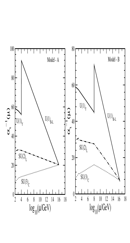
Figure 4.1: Evolution of the gauge couplings in models with additional light multiplets. The left- (right-) panel corresponds to Model A (Model B).

A very precise unification of the gauge couplings has been found when further small SUSY threshold effects at the TeV scale are taken into account [69]. Because of these effects, the resulting gauge couplings show small discontinuities at $M_{S}=10^{3}$ GeV as shown in the Fig. 4.1 for Model B. The gauge couplings near the GUT scale approach strong coupling ($\alpha_{G}\simeq 0.1$) as shown in Table 4.4 and Fig. 4.1.

We show in the next section that the intermediate scale in the triplet model has a lower bound at $10^{9}$ GeV which is expected to be increased by additional Higgs scalars at the $M_{R}$ scale.

From the above two examples and earlier investigations it is clear that right-handed mass scales as low as $M_{R}=5$ TeV $-10^{10}$ GeV are viable when additional light chiral multiplets at the $M_{R}$ scale are admitted. As already noted, such low scales are necessary for the successful implementation of leptogenesis in the doublet model (Model I). Obviously, these models may have interesting new signatures at LHC and future collider experiments. It is noteworthy that all the light multiplets exploited in the two models are contained in $SO(10)$ representations which have been invoked in the literature anyway for various purposes.

4.4 Lower bound on intermediate scale in the triplet model

As pointed out earlier, the higher dimensional Higgs representations like ${\bf{210}}$ and/or ${\bf{126}+\overline{126}}$ result in large threshold corrections at the GUT scale even if their superheavy components are only few times heavier or lighter than $M_{U}$. In this respect, threshold corrections in the triplet model with ${\bf{126}+\overline{126}}$ are more significant compared to those in the doublet model which uses ${\bf{16}+\overline{16}}$. Normally, one would therefore expect to obtain lower $M_{R}$ in the former model.

In this section we show that this is not true and, in fact, establish that $M_{R}$ cannot be lower than $10^{9}$ GeV in the triplet model. This lower bound is set by the perturbative renormalization group constraint when parity survives in the left-right gauge group as happens in the case of $\cal{G}_{LR}$. As the GUT threshold effects contribute only at the unification scale, we use the two-loop equation for $\alpha_{BL}$ between $M_{R}$ and $M_{U}$ with the corresponding coefficients given in eq. (4.21) and eq. (4.48). It is seen that if $M_{R}\leq 10^{9}$ GeV, $\alpha_{BL}$ exceeds the perturbative limit ($\simeq 1$) before the GUT scale is reached.

Analytically, this behavior of the gauge coupling becomes transparent by noting that the position of the Landau pole ($\mu_{0}$), where $g_{BL}(\mu_{0})=\infty$, is given by,

$$\mu_{0} = M_{R}~{}\exp\left[{2\pi\over a^{\prime}_{BL}}{1\over\alpha_{BL}(M_{R})}\right].$$ (4.134)

Here

$${1\over\alpha_{BL}(M_{R})}={5\over 2}\left({1\over\alpha_{Y}(M_{Z})}-\Theta_{Y}+\Delta_{Y}\right)-{3\over 2}\left({1\over\alpha_{2L}(M_{Z})}-\Theta_{2L}+\Delta_{2L}\right)$$

$$-{1\over 4\pi}\left(5a_{Y}-3a_{2L}\right)\ln{M_{R}\over M_{Z}}.$$ (4.135)

Using eq. (4.135) we calculate $\alpha_{BL}^{-1}(M_{R})$ for $M_{R}=10^{3}$ GeV to $10^{11}$ GeV from low energy data ignoring the small threshold effect due to superpartners and use them in eq. (4.134) to estimate the value of $\mu_{0}$. Our two-loop estimations of the pole position are shown in Table 4.5 for the triplet model with $a^{\prime}_{BL}=24$.

$M_{R}$	$\alpha^{-1}_{BL}(M_{R})$	$\mu_{0}$
(GeV)		(GeV)
$10^{3}$	$97.429$	$7.76\times 10^{13}$
$10^{5}$	$86.407$	$4.56\times 10^{14}$
$10^{7}$	$75.406$	$2.56\times 10^{15}$
$10^{8}$	$69.907$	$6.16\times 10^{15}$
$10^{9}$	$64.409$	$1.44\times 10^{16}$
$10^{10}$	$58.912$	$3.46\times 10^{16}$
$10^{11}$	$53.415$	$8.31\times 10^{16}$

Table 4.5: Location of Landau poles, $\mu_{0}$, signifying violation of perturbativity, for different choices of the intermediate scale $M_{R}$ in the triplet model.

The two-loop corrections predict slightly lower values of $\mu_{0}$ than eq. (4.134). For intermediate scales $M_{R}=1$ TeV to $10^{9}$ GeV, the pole positions are found in the range $7.76\times 10^{13}$ GeV to $1.44\times 10^{16}$ GeV indicating that for the $U(1)_{BL}$ gauge coupling perturbation theory breaks down below the GUT scale for these values of $M_{R}$. When $M_{R}\mathop{\smash{>}}\limits_{\sim}10^{10}$ GeV, the pole positions occur clearly above the GUT scale with $\mu_{0}\mathop{\smash{>}}\limits_{\sim}3.46\times 10^{16}$ GeV. In other words, with only the minimal particle content needed to maintain supersymmetry and left-right symmetry below the GUT scale, from the requirement of perturbativity the triplet model leads to the conservative lower bond on the intermediate scale,

$$M_{R}>10^{9}~{}{\rm GeV}.$$ (4.136)

Inclusion of additional new scalar degrees of freedom anywhere between $M_{R}$ to $M_{U}$ would increase the one-loop beta-function coefficient of the $U(1)_{B-L}$ gauge coupling and bring down the pole position further. This, in turn, would further tighten the lower bound on $M_{R}$ beyond $10^{9}$ GeV. This is why, unlike in the doublet model, the presence of additional light scalars near $M_{R}$ cannot reduce the value of the intermediate scale in the triplet model.

In contrast to the triplet model for which $a^{\prime}_{BL}=24$, the doublet model has $a^{\prime}_{BL}=9$ which enhances the argument of the exponential on the RHS of eq. (4.134) by a factor $\simeq 24/9=2.66$ compared to the triplet model for the same value of $M_{R}$. Such a factor in the argument pushes the Landau pole to a position much above the GUT scale. Thus, even with $M_{R}=1$ TeV, whereas the triplet model pole position is at $\mu_{0}\simeq 1.18\times 10^{14}$ GeV which is approximately two orders below the GUT scale, in the the doublet model the pole occurs at $\mu_{0}\simeq 3.3\times 10^{32}$ GeV. Although this latter scale for the doublet model is expected to be substantially lower because of the contribution of superheavy particles near the GUT scale, it is clear that the coupling constant never hits a Landau pole below the GUT-Planck scales $\simeq 10^{18}$ GeV. This tallies with the results in sec. 4.3 where solutions have been obtained using threshold and gravitational corrections.

With such a lower bound on $M_{R}$ in the triplet model, this version of SUSY $SO(10)$ rightly deserves its description as a high scale theory. The SUSY $SO(10)$ triplet model appears to fit ideally for description of quark-lepton masses and mixings through high-scale $b-\tau$ unification and type II see-saw dominance or even through type I see-saw mechanism [75, 77, 85] .

Since $M_{R}\mathop{\smash{>}}\limits_{\sim}10^{9}$ GeV in the triplet model, the lightest right-handed neutrino mass could satisfy the gravitino constraint, but in this case generating the quark and lepton masses and mixings has to be re-examined. While a detailed analysis of neutrino data is yet to emerge in the doublet model, it is well known that reproducing small neutrino masses is no problem even if the right-handed neutrinos are near the TeV scale. With such a low value of $M_{R}$ the desired criteria of TeV scale resonant leptogenesis is fulfilled and through the $W_{R}^{\pm}$ and $Z_{R}$ bosons and the light Higgs scalars, $\chi_{L}^{\pm},\chi_{L}^{0}$, $\chi_{R}^{\pm}$, and $\chi_{R}^{0}$, the model can be tested at the LHC and ILC. The superpartner of the lightest right-handed neutrino in the doublet model may also be a good candidate for dark matter.

4.5 Remarks on light scalars and fermion masses in minimal $SO(10)$

One of the most appealing features of the minimal supersymmetric $SO(10)$ model is that one can calculate the pattern of symmetry breaking and predict fermion mass relations at the GUT scale [86]. Concomitant with these, in the minimal model, is an intermediate left-right breaking scale, $M_{R}$, constrained to be rather close to the GUT scale $M_{U}$. Can the virtues of the model be made to survive when $M_{R}$ is lowered?

Let us briefly summarize the salient features with reference to Model II. The Higgs fields are:

$$\Phi\equiv{\bf 210},~{}~{}~{}~{}~{}\Sigma\equiv{\bf 126},~{}~{}~{}~{}~{}\bar{\Sigma}\equiv{\bf\overline{126}},~{}~{}~{}~{}~{}H\equiv{\bf 10},$$

where $\Delta_{L,R}\subset\Sigma$ and $\phi\subset H$. The fermions belong to the representation $\Psi\equiv$ 16. The complete superpotential of the model can then be written as

$$W=W_{Y}+W_{H},$$ (4.137)

where the Yukawa couplings are in $W_{Y}$ and the scalar potential can be derived from $W_{H}$. They can be written as (we follow the notations of ref. [74])

$$W_{Y} = Y_{10}\Psi\Psi H+Y_{126}\Psi\Psi\bar{\Sigma},$$

$$W_{H} = {m_{\Phi}\over 4!}\Phi\Phi+{\lambda\over 4!}\Phi\Phi\Phi+{M\over 5!}\Sigma\bar{\Sigma}+{\eta\over 4!}\Phi\Sigma\bar{\Sigma}$$ (4.138)

$$+m_{H}HH+{1\over 4!}\Phi H~{}(\alpha\Sigma+\beta\bar{\Sigma}).$$

As usual, minimization of the scalar potential gives the allowed values of the $vev$ of the different fields. In addition, fermion mass relations are also determined in terms of the parameters of the model.

It may appear that the solutions presented earlier with lowered left-right symmetry breaking scales are in conflict with results on fermion masses. However, this need not be the case. For example, when gravitational corrections are included, there may well be non-renormalizable terms in the superpotential, suppressed by the Planck scale, which can contribute to the Yukawa couplings after the GUT symmetry breaking by the field $\Phi$. Thus, in the presence of such corrections, the superpotential will have to be supplemented by

$$W_{Y}^{G}={1\over M_{Pl}}(Y^{G}_{10}\Psi\Psi H\Phi+Y^{G}_{126}\Psi\Psi\bar{\Sigma}\Phi)+\cdots.$$ (4.139)

These new interactions will be suppressed by ${\langle\Phi\rangle/M_{Pl}}$. But $\langle\Phi\rangle\sim M_{U}$ is close to the Planck scale, as we have illustrated, and hence the suppression need not be too much. In addition, the non-renormalizable couplings $Y^{G}$ could also be large. Then the fermion mass relations obtained for the minimal supersymmetric $SO(10)$ models could be radically affected. Fermion mass relations can also get changed in the presence of new Higgs scalars. Thus the low intermediate mass scales, $M_{R}$, obtained in the present analysis need not be inconsistent with the fermion mass relations.

At the tree level, the minimal triplet model predicts  [74] masses near $M_{R}$ for additional states belonging to ${\bf 210}$ with the quantum numbers

$$E_{L}(3,3,1,4/3)\oplus{\overline{E}}_{L}(\overline{3},3,1,-4/3),$$

$$E_{R}(3,1,3,4/3)\oplus{\overline{E}}_{R}(\overline{3},1,3,-4/3).$$ (4.140)

We have checked that with the minimal Higgs content, the renormalizable doublet model also leads to similar light Higgs scalars. It has been further noted in ref. [74] that these states prevent having parity conserving ${\cal G}_{LR}$ at any value of the intermediate scale below $M_{U}$. We remark that their presence at $M_{R}$ sufficiently lower than $M_{U}$, apart from being in conflict with $\sin^{2}\theta_{W}(M_{Z})$ and $\alpha_{S}(M_{Z})$, spoils perturbative gauge coupling evolutions by developing Landau poles in the coupling constants in the region $M_{R}<\mu<M_{U}$. This difficulty could be avoided by extensions of the minimal doublet or the triplet model through the inclusion of non-renormalizable operators and/or additional $SO(10)$ Higgs representations, like $\bf{54}$. For example, the presence of the non-renormalizable term in the superpotential

$$W_{gr} = {\lambda^{G}\over{4!M_{G}}}\Phi^{4},$$

with $M_{G}=M_{Pl}$, or (string) compactification scale, can lift the masses of these light scalars close to the GUT scale when the ${\bf 210}$ gets $vev$ along the direction $\langle\Phi^{0}\{15,1,1\}\rangle~{}\sim~{}M_{U}$, leading to $M_{E}={{2\lambda^{G}m_{\Phi}^{2}}/{\lambda^{2}{M_{G}}}}$. Then their contributions are added to GUT-threshold effects, as discussed earlier.

4.6 Summary and conclusion

In this chapter we have discussed the question of low intermediate left-right symmetry breaking scales, as preferred by leptogenesis, in the minimal supersymmetric $SO(10)$ GUTs with only doublet Higgs scalars as well as with triplet scalars. In view of the presence of additional scalar components predicted from mass spectra analysis [74] which disrupt perturbativity and gauge coupling unification, the minimal renormalizable triplet model with Higgs representations ${\bf 210\oplus 126\oplus{\overline{126}}\oplus 10}$ is ruled out as a candidate for any value of left-right symmetry breaking intermediate scale. With the added presence of a Higgs representation ${\bf 54}$ and/or non-renormalizable interactions, these unwanted scalar components are made superheavy and we find, in agreement with previous work, that in the minimal models, at the one-loop level gauge coupling unification requires the scale of left-right symmetry breaking to be close to the GUT scale . Inclusion of the two-loop contributions eliminates even this possibility as no solution can be found at all with an intermediate scale. On the other hand, evading the gravitino problem, which would otherwise plague successful big bang nucleosynthesis, would require $M_{R}\leq 10^{9}~{}{\rm GeV}$. We have pointed out that this impasse can be circumvented in the case of the doublet model by including threshold corrections near the GUT scale, including non-renormalizable interactions due to gravity induced Planck scale effects, or by adding new light scalar multiplets. In the last alternative, the additional light submultiplets used are present in representations commonly used in $SO(10)$ non-minimal models, but they are different from those which emerge from mass spectra analysis [74]. These considerations allow the left-right symmetry breaking scale to be low, as low as even a few TeV, making it phenomenologically interesting. The unification scale obtained in the doublet model using the first two methods turns out to be large, making it safe for Higgsino mediated proton decay as well as with fermion mass relations. In the triplet model, although threshold effects can easily decrease the intermediate scale, we find a perturbative lower bound, $M_{R}>10^{9}$ GeV, below which the intermediate scale cannot be lowered. With this bound, the triplet model with an added ${\bf 54}$ and/or nonrenormalizable interactions emerges as a high scale theory of SUSY $SO(10)$ description of fermion masses and mixings. In this model the possibility of meeting the gravitino constraint can be fulfilled provided neutrino masses and mixings are successfully reproduced with $M_{R}\mathop{\smash{>}}\limits_{\sim}10^{9}$ GeV. With $M_{R}$ in the TeV region in the doublet model, apart from successful resonant leptogenesis with full compliance of the gravitino constraint, the model predictions can be tested through their various manifestations at the LHC and ILC.

Chapter 5 $SU(6)$, Triquark states, and the pentaquark

5.1 Introduction

Since long, baryon spectroscopy has been an arena to learn about low-energy quantum chromodynamics. The purported observation of a narrow baryon state of strangeness +1 at a mass around 1540 MeV, $\Theta^{+}$, by several experiments [87] brought renewed attention to this theatre. The evidence in support of this new state is now of conflicting nature, loaded more in the direction of non-observation [88, 89]. Within the quark picture, the positive strangeness ($\equiv\bar{s}$) of the $\Theta^{+}$ baryon puts it in an exotic category and entails an interpretation in terms of a minimum of four quarks and an antiquark – a pentaquark state ($udud\bar{s}$).

Soon after, three other states which also demand a pentaquark classification were also observed. These are the $\Xi^{--}(dsds\bar{u})$ and $\Xi^{0}(dsus\bar{d})$ both at 1862 MeV [90] and the $\Sigma^{c}(udud\bar{c})$ [91] with mass 3099 MeV.

Though exotic states such as the pentaquark have a long history, particular attention was drawn to a possible $\Theta^{+}$-like state in the $SU(3)$ version of the chiral soliton model [92]. Subsequently, the experimental results have stimulated the exploration of many ideas, e.g., quark clusters, colour hyperfine interactions, Goldstone boson exchange, QCD sum rules, lattice methods, etc., which have been reviewed in the literature [93].

For the $\Theta^{+}$, within the quark model framework, two models [94, 95] have achieved special prominence. It is convenient to discuss these using the language of $SU(6)$ of colour-spin, $SU(3)$ of colour, and $SU(2)$ of spin. Thus, for example, a quark transforms as (6,3,2), where the three integers within the parentheses identify the representations of the above $SU(6)$, $SU(3)$, and $SU(2)$, respectively. To avoid cluttering, the flavour $SU(3)$ structure is not explicitly shown. Our interest will be on the triquark state which is an ingredient of the Karliner-Lipkin model [94].

An alternative possibility is the Jaffe–Wilczek (JW) model [95]. Here the four quarks are assumed to form two diquark clusters, each in the $(21,\bar{3},1)$ representation. Of the four possible combinations for a two-quark cluster – (21,6,3), (15,6,1), $(15,\bar{3},3)$, $(21,\bar{3},1)$ – this is the one of the lowest energy. The two diquark clusters and the remaining antiquark – each one of which is in colour $\bar{3}$ – combine to form the colour singlet pentaquark state $(qq)(qq)(\bar{q})$, e.g., $\Theta^{+}\equiv(ud)(ud)(\bar{s})$. A relative orbital angular momentum, L=1, is assumed between the diquarks; this is in tune with the observed narrow width of the state. Another consequence is that the pentaquark parity is predicted to be positive. Note that the colour-spin symmetric nature of the $(21,\bar{3},1)$ diquark requires it to be antisymmetric, $\bar{3}$, in flavour to satisfy the generalized Pauli principle. The two diquarks (colour $\bar{3}$ bosons) combine to form colour 3 to match up with the antiquark. This, and L=1, requires the combination to be in a flavour symmetric $\bar{6}$ state. The overall pentaquark flavour must be in $\bar{6}\otimes\bar{3}=8+\overline{10}$. The quantum numbers of $\Theta^{+}$ can be accommodated only in the $\overline{10}$.

In the Karliner-Lipkin (KL) model the quark clustering is different. Here, it is postulated that there is one diquark cluster with the same quantum numbers as in the JW model. The difference is that the remaining two quarks and the antiquark are assumed to form a triquark cluster $(qq\bar{q})$ with the quantum numbers (6,3,2) which is in a flavour $\bar{6}$. The pentaquark state is the colour singlet $(qq)(qq\bar{q})$ combination. To explain the narrowness of the observed states, a relative orbital angular momentum, L=1, is postulated between the clusters so that the parity of the state is predicted to be positive in this model as well. The flavour structure of the states is the same as in the JW model.

In this work, we set two goals. First, we take a detailed look at the group theoretic properties of the triquark state. We derive expressions for the $SU(6)$ unitary scalar factors and Racah coefficients related to the Clebsch-Gordan coefficients relevant for this state [96]. Second, we use these results to estimate masses for pentaquark states. We indicate how flavour symmetry breaking may be incorporated in the analysis.

In the next section we present the $SU(6)$ unitary scalar factors and Racah coefficients, which have been derived ab initio. In section 5.3 we recall the nature of the colour-spin hyperfine interaction while in the following section we use it to estimate the hyperfine energies for baryons, mesons, diquarks, and triquarks. In section 5.5 the different threads are brought together for estimating pentaquark masses. In section 5.6 we discuss the results. We end in section 5.7 with our conclusions.

5.2 Some group-theoretic results

In this section, we collect some results about $SU(6)$ unitary scalar factors and Racah-like coefficients which will be useful for the subsequent discussion. Though our motivation in obtaining these results is the triquark state, they may find some use in other applications of the $SU(6)$ group.

5.2.1 $SU(6)$ unitary scalar factors

To minimise the complexities, we first summarize the notations. A member of an $SU(2)$ multiplet is denoted by $\{(2I+1),I_{3}\}$; e.g., the $s_{z}=+{1\over 2}$ state of a spin-half particle is $\{{2},+{1\over 2}\}$.

For $SU(3)$, the sub-representations are designated by the $SU(2)^{c}$ representation and the ‘hypercharge’, $Y^{c}$. Thus, one uses the combination $\{R_{3},\alpha,I_{3}^{c}\}$ where $R_{3}$ is the $SU(3)$ representation and $\alpha\equiv[(2I^{c}+1),Y^{c}]$. For illustration, a quark state with $I_{3}^{c}=+{1\over 2}$ and $Y^{c}={1\over 3}$ will be denoted as $\{3,[{2},{1\over 3}],+{1\over 2}\}$.

Putting the above together, an $SU(6)$ state is denoted by $(R_{6},\{R_{3},\alpha,I_{3}^{c}\},\{(2I+1),I_{3}\})$ where $R_{6}$ is the $SU(6)$ representation while $\{R_{3},\alpha,I_{3}^{c}\}$ and $\{(2I+1),I_{3}\}$ characterize the corresponding $SU(3)$ and $SU(2)$ sub-representations. The quark state mentioned above, will be $(6,\{3,[{2},{1\over 3}],+{1\over 2}\},\{{2},\pm{1\over 2}\})$, where the $SU(3)$ ($SU(2)$) quantum numbers are enclosed in the first (second) braces. In most of the following, it will be possible to suppress $\alpha,I_{3}^{c}$ and $I_{3}$ – e.g., the quark state $\equiv$ (6,3,2). This is because the unitary scalar factors and the Racah coefficients are independent of $\alpha,I_{3}^{c}$ and $I_{3}$.

The $SU(6)$ unitary scalar factors are generalisations of the $SU(3)$ isoscalar factors. The Clebsch-Gordan (CG) coefficients of $SU(2)$ are well known. If $i\otimes j=k\oplus\ldots$, where $i,j,k$ are $SU(2)$ representations, we use $CG(SU(2)_{i,j,k})$ as an abbreviation for the usual $C^{i,j,k}_{i_{3},j_{3},k_{3}}$ [97].

Using the $SU(2)$ submultiplets within an $SU(3)$ representation, the CG coefficients for $SU(3)$ can be expressed in terms of products of isoscalar factors and $SU(2)$ CG coefficients. Schematically, for the case $P\otimes Q=R\oplus\ldots$:

$$CG(SU(3)_{P,Q,R})=\left[\matrix{P&Q&R\cr\alpha_{P}&\alpha_{Q}&\alpha_{R}}\right]\times CG(SU(2)_{I_{P},I_{Q},I_{R}}),$$ (5.1)

where the $\alpha_{i},~{}i=P,Q,R$ indicate the sub-representations of the $SU(3)$ representations $P,Q,R$. The first factor on the right-hand-side is the $SU(3)$ isoscalar factor. It is independent of $I_{P3},I_{Q3},I_{R3}$. Tables of $SU(3)$ isoscalar factors have been available for long [98].

Similarly, in $SU(6)$, if $X\otimes Y=Z\oplus\ldots$ then

$$CG(SU(6)_{X,Y,Z}) = \left[\matrix{X&Y&Z\cr(P_{X},I_{X})&(P_{Y},I_{Y})&(P_{Z},I_{Z})}\right]$$ (5.2)

$$\times CG(SU(3)_{P_{X},P_{Y},P_{Z}})\times CG(SU(2)_{I_{X},I_{Y},I_{Z}}).$$

Here, the first factor on the right-hand-side is an $SU(6)$ unitary scalar factor – the generalization of the $SU(3)$ isoscalar factor. $P_{X}(I_{X})$ indicates the $SU(3)$ ($SU(2)$) sub-representation within the $SU(6)$ multiplet $X$.

Since the triquark state is made out of two quarks ($q_{1},q_{2}$) and an antiquark ($\bar{q}_{3}$), the following $SU(6)$ combinations arise:

$$qq{\rm~{}state:~{}~{}}6\otimes 6=21\oplus 15$$ (5.3)

$$qq\bar{q}{\rm~{}state:~{}~{}}21\otimes\bar{6}=120\oplus 6_{1}^{\phi},\;\;15\otimes\bar{6}=84\oplus 6_{2}^{\phi}.$$ (5.4)

or, alternatively,

$$q\bar{q}{\rm~{}state:~{}~{}}6\otimes\bar{6}=35\oplus 1$$ (5.5)

$$q\bar{q}q{\rm~{}state:~{}~{}}35\otimes 6=120\oplus 84\oplus 6_{1}^{\psi},\;\;1\otimes 6=6_{2}^{\psi}.$$ (5.6)

The superscripts $\phi$ and $\psi$ will be clarified in the next subsection where we identify the Racah coefficients which relate $(6_{1}^{\phi},6_{2}^{\phi})$ to $(6_{1}^{\psi},6_{2}^{\psi})$.

For the purpose of the triquark, the $SU(6)$ CG coefficients for the product 21 $\otimes$ $\bar{6}$ = 120 $\oplus$ 6 are necessary. We have not been able to find the $SU(6)$ unitary scalar factors for this product in the published literature [99]. Here, therefore, their ab initio calculated values are presented. We follow the generalized Condon-Shortley phase convention [100] and obtain:

$$\left[\matrix{21&\overline{6}&6\cr(6,3)&(\overline{3},2)&(3,2)}\right]=\sqrt{6\over 7},\;\;\;\left[\matrix{21&\overline{6}&6\cr(\overline{3},1)&(\overline{3},2)&(3,2)}\right]=\sqrt{1\over 7}.$$ (5.7)

Also,

$$\left[\matrix{21&\overline{6}&120\cr(6,3)&(\overline{3},2)&(3,2)}\right]=\sqrt{1\over 7},\;\;\;\left[\matrix{21&\overline{6}&120\cr(\overline{3},1)&(\overline{3},2)&(3,2)}\right]=-\sqrt{6\over 7}.$$ (5.8)

For the sake of completeness, the $SU(6)$ unitary scalar factors for the case 15 $\otimes$ $\bar{6}$ = 84 $\oplus$ 6 are:

$$\left[\matrix{15&\overline{6}&6\cr(6,1)&(\overline{3},2)&(3,2)}\right]=\sqrt{2\over 5},\;\;\;\left[\matrix{15&\overline{6}&6\cr(\overline{3},3)&(\overline{3},2)&(3,2)}\right]=\sqrt{3\over 5}.$$ (5.9)

and

$$\left[\matrix{15&\overline{6}&84\cr(6,1)&(\overline{3},2)&(3,2)}\right]=\sqrt{3\over 5},\;\;\;\left[\matrix{15&\overline{6}&84\cr(\overline{3},3)&(\overline{3},2)&(3,2)}\right]=-\sqrt{2\over 5}.$$ (5.10)

5.2.2 Racah coefficients for the triquark cluster

$SU(2)$ and $SU(3)$

In this subsection, after recapitulating the concept of Racah coefficients, using angular momentum as an illustration, the necessary results useful for the triquark case are presented.

When three angular momenta $j_{1},j_{2},j_{3}$ are added, one can obtain the same final angular momentum $j$ by, for example, (a) combining $j_{1}$ and $j_{2}$ first to get $j_{12}$ and adding $j_{3}$ to it, or by (b) first adding $j_{1}$ and $j_{3}$ to obtain $j_{13}$ and then combining it with $j_{2}$, or by (c) adding $j_{2}$ and $j_{3}$ to obtain $j_{23}$ and then adding $j_{1}$ to it. The states of the representation $j$ obtained by these three different routes, may be denoted by $|j_{1},j_{2},j_{3};j_{12},j,m\rangle$, $|j_{1},j_{2},j_{3};j_{13},j,m\rangle$, and $|j_{1},j_{2},j_{3};j_{23},j,m\rangle$, respectively. These three sets of states are related to each other by unitary transformations whose coefficients, $U$, are called the normalized Racah coefficients. For example,

$$U(j_{1},j_{2},j_{3},j;j_{12},j_{13})=\langle j_{1},j_{2},j_{3};j_{12},j,m|j_{1},j_{2},j_{3};j_{13},j,m\rangle.$$ (5.11)

The triquark state is of the structure ($q_{1}q_{2}\bar{q}_{3}$). Since the quarks (antiquarks) transform as 6 ($\bar{6}$) of colour-spin $SU(6)$, for the analysis of these states one requires the Racah coefficients for $SU(6)$ for the product $6\times 6\times\bar{6}$.

For most purposes, it actually suffices if one has the colour $SU(3)$ and spin $SU(2)$ Racah coefficients.

The same final triquark state may be reached by first combining $q_{1}$ and $q_{2}$ (colour: $3\times 3=\bar{3}+6$ and spin: $2\times 2=3+1$) and then combining with each of these possibilities the antiquark state $\bar{q}_{3}$. An alternate way of obtaining the same state is to first pair $q_{1}$ with $\bar{q}_{3}$ (colour: $3\times\bar{3}=8+1$ and spin: $2\times 2=3+1$) and then adjoining $q_{2}$ to the result. A third possibility is obtained by interchanging $q_{1}\leftrightarrow q_{2}$ in the previous alternative.

We concentrate, in the interest of the pentaquark application, on the triqark state which transforms like a colour $SU(3)$ triplet and an $SU(2)$ doublet. The basis states in this sector may be denoted as:

$$\left(\matrix{|\phi_{1}\rangle\cr|\phi_{2}\rangle\cr|\phi_{3}\rangle\cr|\phi_{4}\rangle\cr}\right)\equiv\left(\matrix{|(q_{1}q_{2})^{\bar{3}}_{1}(\bar{q}_{3})^{\bar{3}}_{2}\rangle_{(3,2)}\cr|(q_{1}q_{2})^{6}_{1}(\bar{q}_{3})^{\bar{3}}_{2}\rangle_{(3,2)}\cr|(q_{1}q_{2})^{\bar{3}}_{3}(\bar{q}_{3})^{\bar{3}}_{2}\rangle_{(3,2)}\cr|(q_{1}q_{2})^{6}_{3}(\bar{q}_{3})^{\bar{3}}_{2}\rangle_{(3,2)}\cr}\right)$$ (5.12)

and

$$\left(\matrix{|\psi_{1}\rangle\cr|\psi_{2}\rangle\cr|\psi_{3}\rangle\cr|\psi_{4}\rangle\cr}\right)\equiv\left(\matrix{|(q_{1}\bar{q}_{3})^{1}_{1}(q_{2})^{3}_{2}\rangle_{(3,2)}\cr|(q_{1}\bar{q}_{3})^{8}_{1}(q_{2})^{3}_{2}\rangle_{(3,2)}\cr|(q_{1}\bar{q}_{3})^{1}_{3}(q_{2})^{3}_{2}\rangle_{(3,2)}\cr|(q_{1}\bar{q}_{3})^{8}_{3}(q_{2})^{3}_{2}\rangle_{(3,2)}\cr}\right),\;\;\;\left(\matrix{|\chi_{1}\rangle\cr|\chi_{2}\rangle\cr|\chi_{3}\rangle\cr|\chi_{4}\rangle\cr}\right)\equiv\left(\matrix{|(q_{2}\bar{q}_{3})^{1}_{1}(q_{1})^{3}_{2}\rangle_{(3,2)}\cr|(q_{2}\bar{q}_{3})^{8}_{1}(q_{1})^{3}_{2}\rangle_{(3,2)}\cr|(q_{2}\bar{q}_{3})^{1}_{3}(q_{1})^{3}_{2}\rangle_{(3,2)}\cr|(q_{2}\bar{q}_{3})^{8}_{3}(q_{1})^{3}_{2}\rangle_{(3,2)}\cr}\right).$$ (5.13)

The notation used here, for example, is that the triquark state with $SU(3)$ ($SU(2)$) multiplicity $c^{\prime}$ ($s^{\prime}$) obtained through the diquark combination $(q_{1}q_{2})$ with $SU(3)$ and $SU(2)$ multiplicity $c$ and $s$, respectively, is represented as $|(q_{1}q_{2})^{c}_{s}(\bar{q}_{3})^{\bar{3}}_{2}\rangle_{(c^{\prime},s^{\prime})}$.

These possibilities are related by Racah-like coefficients which are found by explicit calculation to be:

$$\left(\matrix{|\phi_{1}\rangle\cr|\phi_{2}\rangle\cr|\phi_{3}\rangle\cr|\phi_{4}\rangle\cr}\right)=\left(\matrix{-\frac{1}{2\sqrt{3}}&\frac{1}{\sqrt{6}}&\frac{1}{2}&-\frac{1}{\sqrt{2}}\cr\frac{1}{\sqrt{6}}&\frac{1}{2\sqrt{3}}&-\frac{1}{\sqrt{2}}&-\frac{1}{2}\cr\frac{1}{2}&-\frac{1}{\sqrt{2}}&\frac{1}{2\sqrt{3}}&-\frac{1}{\sqrt{6}}\cr-\frac{1}{\sqrt{2}}&-\frac{1}{2}&-\frac{1}{\sqrt{6}}&-\frac{1}{2\sqrt{3}}\cr}\right)\left(\matrix{|\psi_{1}\rangle\cr|\psi_{2}\rangle\cr|\psi_{3}\rangle\cr|\psi_{4}\rangle\cr}\right)$$ (5.14)

and

$$\left(\matrix{|\phi_{1}\rangle\cr|\phi_{2}\rangle\cr|\phi_{3}\rangle\cr|\phi_{4}\rangle\cr}\right)=\left(\matrix{-\frac{1}{2\sqrt{3}}&\frac{1}{\sqrt{6}}&\frac{1}{2}&-\frac{1}{\sqrt{2}}\cr-\frac{1}{\sqrt{6}}&-\frac{1}{2\sqrt{3}}&\frac{1}{\sqrt{2}}&\frac{1}{2}\cr-\frac{1}{2}&\frac{1}{\sqrt{2}}&-\frac{1}{2\sqrt{3}}&\frac{1}{\sqrt{6}}\cr-\frac{1}{\sqrt{2}}&-\frac{1}{2}&-\frac{1}{\sqrt{6}}&-\frac{1}{2\sqrt{3}}\cr}\right)\left(\matrix{|\chi_{1}\rangle\cr|\chi_{2}\rangle\cr|\chi_{3}\rangle\cr|\chi_{4}\rangle\cr}\right).$$ (5.15)

$SU(6)$ Racah coefficients

One can use the unitary scalar factors in eqs. (5.7) - (5.8) to write:

$$|q_{1}q_{2}\bar{q}_{3}\rangle_{(6_{1}^{\phi},3,2)}=\sqrt{6\over 7}~{}|\phi_{4}\rangle+\sqrt{1\over 7}~{}|\phi_{1}\rangle,\;\;|q_{1}q_{2}\bar{q}_{3}\rangle_{(120,3,2)}=\sqrt{1\over 7}~{}|\phi_{4}\rangle-\sqrt{6\over 7}~{}|\phi_{1}\rangle.$$ (5.16)

From eqs. (5.9) - (5.10) the states obtained if the diquarks are in the 15 of $SU(6)$ are:

$$|q_{1}q_{2}\bar{q}_{3}\rangle_{(6_{2}^{\phi},3,2)}=\sqrt{2\over 5}~{}|\phi_{2}\rangle+\sqrt{3\over 5}~{}|\phi_{3}\rangle,\;\;|q_{1}q_{2}\bar{q}_{3}\rangle_{(84,3,2)}=\sqrt{3\over 5}~{}|\phi_{2}\rangle-\sqrt{2\over 5}~{}|\phi_{3}\rangle.$$ (5.17)

Using eq. (5.14) one then has:

$$|q_{1}q_{2}\bar{q}_{3}\rangle_{(6_{1}^{\phi},3,2)}=-\sqrt{7\over 12}|\psi_{1}\rangle-\sqrt{2\over 21}|\psi_{2}\rangle-\sqrt{1\over 28}|\psi_{3}\rangle-\sqrt{2\over 7}|\psi_{4}\rangle$$ (5.18)

and

$$|q_{1}q_{2}\bar{q}_{3}\rangle_{(6_{2}^{\phi},3,2)}=\sqrt{5\over 12}|\psi_{1}\rangle-\sqrt{2\over 15}|\psi_{2}\rangle-\sqrt{1\over 20}|\psi_{3}\rangle-\sqrt{2\over 5}|\psi_{4}\rangle$$ (5.19)

Thus, one arrives at the Racah coefficients:

$$\left(\matrix{|(6_{1}^{\phi},3,2)\rangle\cr|(6_{2}^{\phi},3,2)\rangle}\right)=\left(\matrix{\sqrt{\frac{5}{12}}&-\sqrt{\frac{7}{12}}\cr\sqrt{\frac{7}{12}}&\sqrt{\frac{5}{12}}}\right)\left(\matrix{|(6_{1}^{\psi},3,2)\rangle\cr|(6_{2}^{\psi},3,2)\rangle}\right)$$ (5.20)

The non-trivial unitary scalar factors corresponding to eq. (5.6) can be written as:

$$\left[\matrix{35&6&\alpha\cr i&({3},2)&(3,2)}\right]=U_{i,\alpha},$$ (5.21)

with $i=1,2,3$ corresponding to (8,1), (1,3), and (8,3) while $\alpha=1,2,3$ to 120, 84, and $6_{1}^{\psi}$. Then,

$$U=\left(\matrix{-\sqrt{\frac{9}{28}}&-\sqrt{\frac{8}{21}}&\sqrt{\frac{25}{84}}\cr\sqrt{\frac{9}{20}}&-\sqrt{\frac{8}{15}}&-\sqrt{\frac{1}{60}}\cr-\sqrt{\frac{8}{35}}&-\sqrt{\frac{3}{35}}&-\sqrt{\frac{24}{35}}\cr}\right),$$ (5.22)

Now we turn to the application of these results to the pentaquark.

5.3 Colour-spin hyperfine interaction

Besides colour electric forces between all quarks and antiquarks, there exists a colour-spin hyperfine (colour magnetic) interaction [101]. In the KL model, it is assumed that this interaction is operative inside the clusters but, due to the larger separation, the hyperfine interaction between clusters is negligible. The colour-spin $SU(6)$ hyperfine interaction energy is:

$$V=-\sum_{i>j}v_{ij}(\vec{\sigma_{i}}.\vec{\sigma_{j}})(\vec{\lambda_{i}}.\vec{\lambda_{j}}).$$ (5.23)

Here, $\vec{\sigma}$ and $\vec{\lambda}$ are the Pauli and Gell-Mann matrices, and $i$ and $j$ run over the constituent quarks and antiquarks. The common practice is to take $v_{ij}\equiv v$ (flavour symmetry). $v$ captures information about the radial dependence of the bound state wave-function. For a composite system of $n_{q}$ quarks and $n_{\bar{q}}$ antiquarks, the hyperfine energy contribution is given by:

$$E_{hyp}=\left[D(q+\bar{q})-2D(q)-2D(\bar{q})+16(n_{q}+n_{\bar{q}})\right]v/2,$$ (5.24)

where

$$D(R_{6},R_{3},s)=C_{6}(R_{6})-C_{3}(R_{3})-{8\over 3}s(s+1).$$ (5.25)

$C_{6}$ and $C_{3}$ are the quadratic Casimir operators of $SU(6)$ and $SU(3)$ respectively, and $s$, is the spin of the state. The effect of this hyperfine interaction on multiquark exotic states has been a topic of research over several decades [103, 104].

The mass estimate for the pentaquark proceeds along the following pattern. There are three contributions: (a) the masses of the constituent quarks, (b) the colour-spin hyperfine energy, and (c) the energy due to the P-wave excitation. The practice has been to estimate (a) from the masses of the decay products, (baryon + meson), since their quark content is the same as that of the parent; but here the hyperfine interaction contribution to the baryon and meson mass must be first subtracted out, as detailed in section V. Thus, the hyperfine interaction enters directly in (b) and also indirectly in (a) through the way it is extracted.

5.4 Hyperfine energies

5.4.1 Mesons and Baryons

As noted, the hyperfine interaction contributions to the meson $(q\bar{q})$ and baryon $(qqq)$ masses are required for the estimation of the pentaquark mass. These can be readily calculated using eq. (5.24). For example, in the flavour symmetry limit, one finds:

$$E_{N(70,1,2)}=-8v,\;\;E_{\Delta(20,1,4)}=8v,\;\;E_{\pi(1,1,1)}=-16v,\;\;E_{\rho(35,1,3)}=\frac{16}{3}v,$$ (5.26)

where in the parentheses the $SU(6)$, $SU(3)$, and $SU(2)$ properties of the particle have been indicated.

5.4.2 The diquark cluster

As already mentioned, the diquark $(qq)$ is usually chosen to be in the (21,$\bar{3}$,1) representation which is symmetric in $SU(6)$. In addition, a diquark can be in the (21,6,3), (15,6,1), and (15,$\bar{3}$,3) but these have higher energy. One finds from eq. (5.24) that the hyperfine energies for these four states are:

$$E_{(21,\bar{3},1)}=-8v,\;\;E_{(21,6,3)}=-\frac{4}{3}v,\;\;E_{(15,6,1)}=4v,\;\;E_{(15,\bar{3},3)}=\frac{8}{3}v.$$ (5.27)

5.4.3 The triquark cluster

The triquark cluster in the Karliner-Lipkin model is a member of the (6,3,2) multiplet and contains two quarks and an antiquark. The two quarks are assumed to combine to a symmetric 21 of colour-spin $SU(6)$. For $SU(6)$ 21 $\otimes\bar{6}$ = 6 $\oplus$ 120, and the triquark (120,3,2) carries higher hyperfine energy. If the two quarks are combined in an antisymmetric fashion, producing a 15 of $SU(6)$, then the triquark can be in (6,3,2) or (84,3,2).

More important is the fact that in the existing literature, the triquark in the (6,3,2) is assumed to be made with the two quarks within the cluster forming a (21,6,3). In actuality, so long as flavour symmetry of the hyperfine interaction holds, the lowest energy eigenstate of $SU(6)$ receives contributions from both the $(21,6,3)$ and the $(21,\bar{3},1)$ combinations – see eq. (5.7) – and this triquark has the form given in the first expression in eq. (5.16). The other possible triquark states are the second expression in eq. (5.16) and the ones in eq. (5.17).

The triquark hyperfine energy

The calculation of the triquark hyperfine energy using eq. (5.24) is complicated by the fact that the operator $D(q+\bar{q})$ and $D(q)$ do not commute; e.g., in eq. (5.16) an eigenstate of $D(q+\bar{q})$ is expressed as a linear combination of those of $D(q)$.

To circumvent this difficulty, we use the following procedure. We consider the contribution of eq. (5.23) for the triquark state term by term as:

$$V=V_{12}(\vec{\sigma_{1}}.\vec{\sigma_{2}})(\vec{\lambda_{1}}.\vec{\lambda_{2}})+V_{13}(\vec{\sigma_{1}}.\vec{\sigma_{3}})(\vec{\lambda_{1}}.\vec{\lambda_{3}})+V_{23}(\vec{\sigma_{2}}.\vec{\sigma_{3}})(\vec{\lambda_{2}}.\vec{\lambda_{3}}).$$ (5.28)

The hyperfine energy from each term is most readily calculated in the basis where the two contributing quarks/antiquarks are first combined [105]; i.e., corresponding to the three terms in the r.h.s. of eq. (5.28) these are the $|\phi\rangle$, $|\psi\rangle$, and $|\chi\rangle$ bases of Sec. 5.2, respectively. They are related to each other through eqs. (5.14) and (5.15). In terms of these basis states, one can immediately write down the expectation value of the Hamiltonian in eq. (5.28). Thus, one has:

$$\langle\phi|V|\phi\rangle=\left(\matrix{\frac{4}{3}V_{12}+\frac{20}{3}V^{\phi}_{+}&4\sqrt{2}V^{\phi}_{-}&\frac{10}{\sqrt{3}}V^{\phi}_{-}&2\sqrt{6}V^{\phi}_{+}\cr 4\sqrt{2}V^{\phi}_{-}&-\frac{8}{3}V_{12}+\frac{8}{3}V^{\phi}_{+}&2\sqrt{6}V^{\phi}_{+}&\frac{4}{\sqrt{3}}V^{\phi}_{-}\cr\frac{10}{\sqrt{3}}V^{\phi}_{-}&2\sqrt{6}V^{\phi}_{+}&-4V_{12}&0\cr 2\sqrt{6}V^{\phi}_{+}&\frac{4}{\sqrt{3}}V^{\phi}_{-}&0&8V_{12}\cr}\right),$$ (5.29)

where $V^{\phi}_{\pm}=V_{13}\pm V_{23}$. Analogously,

$$\langle\psi|V|\psi\rangle=\left(\matrix{\frac{8}{3}V_{12}+\frac{2}{3}V_{13}+\frac{28}{3}V_{23}&\frac{16}{3\sqrt{2}}V^{\psi}_{-}&\frac{4}{\sqrt{3}}V_{12}-\frac{14}{\sqrt{3}}V_{23}&\frac{8}{\sqrt{6}}V^{\psi}_{+}\cr\frac{16}{3\sqrt{2}}V^{\psi}_{-}&-\frac{16}{3}V_{13}&\frac{8}{\sqrt{6}}V^{\psi}_{+}&0\cr\frac{4}{\sqrt{3}}V_{12}-\frac{14}{\sqrt{3}}V_{23}&\frac{8}{\sqrt{6}}V^{\psi}_{+}&-2V_{13}&0\cr\frac{8}{\sqrt{6}}V^{\psi}_{+}&0&0&16V_{13}\cr}\right),$$ (5.30)

where $V^{\psi}_{\pm}=V_{12}\pm V_{23}$. $\langle\chi|V|\chi\rangle$ is similar and is not presented here.

The eigenvalues and eigenvectors of this matrix give the triquark energy and its corresponding group theoretic configuration, respectively.

The method which we follow can be smoothly adopted to the case of flavour symmetry violation by appropriately changing the individual coupling strengths in the three terms of eq. (5.28). In the flavour symmetry limit, $V_{12}=V_{23}=V_{13}=v$, whence $V_{-}^{\phi}=V_{-}^{\psi}=0$. It is seen from eq. (5.29) that $(\phi_{1},\phi_{4})$ decouple from $(\phi_{2},\phi_{3})$ in this limit.

5.5 Pentaquark masses

5.5.1 Hyperfine interaction couplings

Needless to say, the strength of the colour-spin hyperfine interaction, $v$, is an important ingredient of the pentaquark mass estimation. The procedure has generally been to assume that it takes a universal value which is estimated by ascribing the $\Delta-N$ mass splitting to this interaction. Using eq. (5.26),

$$v_{3}=\frac{m_{\Delta}-m_{N}}{16}\simeq 18.3\;{\rm MeV}.$$ (5.31)

While this can be a first approximation, it should be borne in mind that $v$ is determined by the radial dependence of the bound state wave-function and thus is most likely different for two-body and three-body bound states. Indeed, using eq. (5.26) for the meson sector one has,

$$v_{2}=\frac{m_{\rho}-m_{\pi}}{64/3}\simeq 29.6\;{\rm MeV}.$$ (5.32)

This is actually an overestimate of $v_{2}$ since it is well known that the pion mass is too small for a simple quark model interpretation. Eq. (5.32) is only for the purpose of illustration. However, it does indicate that it may not be unreasonable to expect that $v_{2}\neq v_{3}$ would give a better approximation to reality. In the following, in addition to discussing the results for the choice $v_{2}=v_{3}$, for the sake of comparison, we also use a $v_{2}$ for the diquarks different from the $v_{3}$ for the triquarks.

5.5.2 Flavour symmetry breaking

In the limit of exact flavour symmetry, the splitting between the lowest lying pseudoscalar mesons and the corresponding vector mesons with the same quark content would be flavour independent. A measure of flavour symmetry breaking can be obtained from

$$x_{f}=\frac{m_{K^{*}}-m_{K}}{m_{\rho}-m_{\pi}}\simeq 0.63.$$ (5.33)

This suggests that the hyperfine interaction involving an $s$-quark or antiquark carries a suppression by the factor $x_{f}$. In eqs. (5.32) and (5.33) the use of $m_{\pi}$ makes the precise values inaccurate. To improve upon this, we use the masses of the heavier mesons $\rho$, $\phi$, $K^{*}$, and $K$. Using eq. (5.26), the hyperfine contributions for these states are, respectively,

$$E_{\rho}=\frac{16}{3}v_{2},\;\;E_{\phi}=\frac{16}{3}x_{f2}^{2}v_{2},\;\;E_{K^{*}}=\frac{16}{3}x_{f2}v_{2},\;\;E_{K}=-16x_{f2}v_{2},$$ (5.34)

Here we have added a subscript to $v$ and $x_{f}$ to indicate that these values of the hyperfine parameters apply for two-quark and/or antiquark systems. Using the masses of the mesons, one can solve for the hyperfine interaction parameters $(v_{2},x_{f2})$ as well as the quark masses. In this manner, one gets:

$$v_{2}=23.62~{}{\rm MeV},\;\;x_{f2}=0.782,\;\;m_{u,d}=322~{}{\rm MeV},\;\;m_{s}=471~{}{\rm MeV}.$$ (5.35)

These values are used in our subsequent calculations.

There are two three-body systems which enter in this analysis. One is the triquark state and the other the baryon to which the pentaquark decays. Just as for mesons, one can estimate the values of $v_{3}$ and $x_{f3}$ from the $N-\Delta$ and $\Sigma-\Sigma^{*}$ mass splittings which are given by:

$$E_{\Delta}-E_{N}=16v_{3},\;\;E_{{\Sigma}^{*}}-E_{\Sigma}=\frac{16}{3}v_{3}(2x_{f3}+1),\;\;E_{{\Xi}^{*}}-E_{\Xi}=\frac{16}{3}v_{3}x_{f3}(x_{f3}+2).$$ (5.36)

As a consistency check, we use the values so obtained to calculate the $\Xi-\Xi^{*}$ splitting and find that the agreement is not satisfactory. Therefore, we use all of the three above splittings to arrive at the best-fit values:

$$v_{3}=17.89~{}{\rm MeV},\;\;x_{f3}=0.708.$$ (5.37)

In the following, these have been used for the triquark and baryons.

5.5.3 P-wave excitation

The energy due to the P-wave excitation can be estimated from the recently observed $D_{s}^{*}$ state at 2317 MeV, which is believed to be an orbital excitation of the state at 2112 MeV. This gives

$$E_{P}=m_{D_{s}^{*}}(P)-m_{D_{s}^{*}}(S)\simeq(2317-2112)\;{\rm MeV}=205\;{\rm MeV}.$$ (5.38)

5.6 Results

5.6.1 The flavour antidecuplet and the octet

Putting together the inputs from the previous sections, one can readily obtain the masses of the pentaquark states in the Karliner-Lipkin model. For example, for $\Theta^{+}$, using eqs. (5.26) and (5.27):

$$m_{\Theta^{+}}=\{(m_{N}+8v_{3})+(m_{s}+m_{q})\}+E_{P}-8v_{2}+E_{tri}(v_{3},x_{f3}),$$ (5.39)

where the expression in the curly brackets is the contribution from the quark masses. The last (penultimate) term is the hyperfine energy of the triquark (diquark). For other pentaquarks, the r.h.s. in eq. (5.39) has to be appropriately modified to reflect the quark content of the state and, when necessary, deviations from flavour symmetry have to be incorporated in eq. (5.28) to obtain the correct $E_{tri}(v_{3},x_{f3})$.

Pentaquark	Mass (in MeV)
states	$\Theta^{+}$	$N_{10}$	$\Sigma_{10}$	$\Xi_{10}$	$N_{8}$	$\Sigma_{8}$	$\Xi_{8}$
Lowest	1601	1358	1626	1783	2057	2217	2326
$SU(6)$ Excited	1789	1573	1840	1966	2321	2439	2512

Table 5.1: Pentaquark lowest lying state and first colour-spin excited state masses for the reference values of the parameters in eqs. (5.35) and (5.37).

As noted earlier, the pentaquark states fill an octet and an antidecuplet of flavour. Excepting for the three states, $\Theta^{+}\equiv udud\bar{s}$, $\Xi^{--}\equiv dsds\bar{u}$, and $\Xi^{+}\equiv usus\bar{d}$, all other states in the antidecuplet have partners in the octet with identical isospin and hypercharge. In estimating the masses, we have assumed ideal mixing between the partners and ascribed the lighter member to the antidecuplet. Note that isospin symmetry is assumed unbroken, so it is enough to present the mass of one member of an isomultiplet. The masses of the pentaquark states at the reference values of the parameters – see eqs. (5.35) and (5.37) – are given in Table 5.1.

In Fig. 5.1, in the left panel the antidecuplet pentaquark masses are shown as a function of the flavour symmetry violation parameter $x_{f}$, which assumes the value unity in the symmetry limit. In view of the closeness of the estimates of $x_{f}$ in eqs. (5.35) and (5.37), for this figure we have taken $x_{f3}=x_{f2}=x_{f}$. The triquark interaction strength has been kept fixed at $v_{3}=17.89$ MeV. The bands arise from a variation of the strength of the diquark hyperfine interaction, $v_{2}$, with the lower edge corresponding to $v_{2}=v_{3}$ and the upper to $v_{2}=23.62$ MeV (see eq. (5.35)). For this figure, $E_{P}$ has been chosen as 209 MeV, following eq. (5.38). It is observed that the triquark corresponding to the lowest eigenvalue of the hyperfine energy Hamiltonian – eq. (5.29) – is predominantly a combination of the states $\phi_{1}$ and $\phi_{4}$ (see eq. (5.12)) which are antisymmetric in the quark flavours.

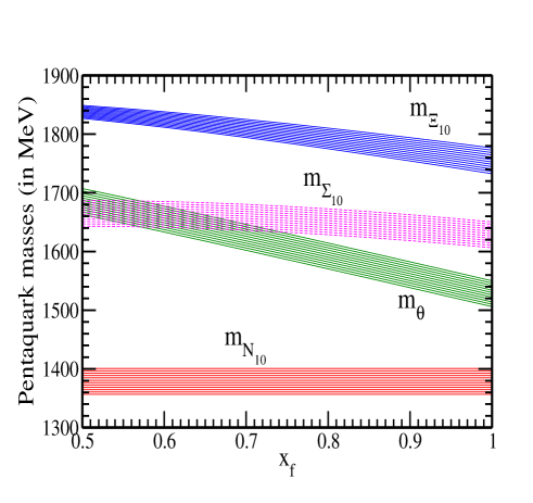
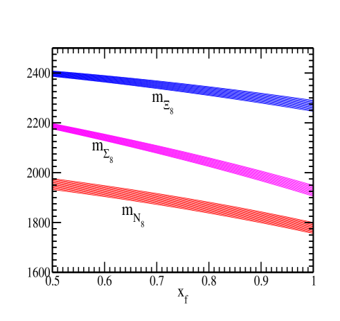
Figure 5.1: Dependence of pentaquark masses on the deviation from flavour symmetry ($x_{f}=1$). The left (right) panel corresponds to flavour antidecuplet (octet) pentaquarks. The bands are obtained when the diquark hyperfine interaction strength is varied over the range 17.89 MeV $\leq v_{2}\leq 23.62$ MeV (see text).

Note that, $N_{10}$, the non-strange member of the antidecuplet is predicted to be at a mass of 1355 MeV for $v_{2}=v_{3}$ which is enhanced to $\sim$ 1400 MeV when $v_{2}=23.62$ MeV is used. This prediction is independent of the choice of $x_{f}$ since the state does not have strange quarks. For the exotic $\Xi^{--}_{10}$ state the mass prediction is in the range 1795 – 1825 MeV for $x_{f}$ = 0.7 to be compared with that of the experimentally observed state at 1862 MeV [90].

In the right panel of Fig. 5.1 are shown the octet pentaquark masses. The splitting between the masses of the octet states and the corresponding antidecuplet states is seen to be typically around 500-600 MeV. As noted earlier, at the level of these calculations, the masses of the I=1 and I=0 members of the octet with S = -1 are the same. The non-strange neutral state in the octet, $N_{8}^{0}$, has the quark structure $(ud\bar{s})(ds)$ and its mass is consequently dependent on $x_{f}$.

A remark needs to be made about the symmetry property of the triquark state for the octet pentaquarks. This feature is most easily brought out from a consideration of the S = -2 member of the octet, $\Xi_{8}$, which has the quark structure $(us)(ss\bar{s})$. The diquark is antisymmetric in flavour so its choice is fixed. Unlike all the other states, here the triquark is compelled to have two identical ($s$) quarks, besides the antiquark. Consequently, in the notation of section II, it can arise only from a combination of the states $\phi_{2}$ and $\phi_{3}$ (see eq. (5.12)) which are symmetric in flavour. Obviously, all states in the pentaquark octet will share this feature in the exact flavour $SU(3)$ limit.

The H1 experiment at HERA found evidence of a possible charmed pentaquark at mass 3099 MeV [91]. This state has the quantum numbers of a pentaquark with the structure $udud\bar{c}$. Including flavour violation ($x_{f}=0.23$ for the $\bar{c}$ quark) and taking $v_{2}$ = 23.62 MeV, $v_{3}$ = 17.89 MeV, we find the predicted mass for such a state is 2757 MeV.

5.6.2 Triquark $SU(6)$ excitations

Colour triplet, spin $\frac{1}{2}$ triquarks come in four varieties. These are the four eigenstates of the hyperfine energy matrix in eq. (5.29). The results presented so far are obtained using the eigenstate with the minimum energy consistent with symmetry requirements – a certain choice of colour-spin assignments for the quark clusters – and leads to the lowest lying pentaquarks. It is evident that the other triquark eigenstate clusters also lead to colour singlet spin $1\over 2$ pentaquark states, albeit heavier. How different are the masses in these other cases?

For illustration, we show in Table 5.1 the masses of the first excited partners of the antidecuplet and octet pentaquarks for the reference values of the hyperfine interaction parameters. In the flavour symmetry limit ($x_{f3}=x_{f2}$ = 1), the spacing between the excited states is independent of the flavour and the lowest and first excited states are separated by 215 MeV (370 MeV) for every member of the antidecuplet (octet).

There is no obvious argument to suppress the production of these additional states. It will be of interest to extend the ongoing searches to look for such $SU(6)$ colour-spin excited partners, a novelty of QCD and the pentaquark system.

5.7 Conclusions

A pentaquark interpretation of the $\Theta^{+}$ leads to predictions of several other colour singlet states in a similar mass range which populate an antidecuplet and an octet of flavour $SU(3)$. In this work, the masses of these pentaquark states have been calculated in a triquark-diquark (Karliner-Lipkin) model with refined estimates, up to first order, of the color-spin $SU(6)$ hyperfine interaction contributions.

Motivated by the structure of these states, the $SU(6)$ unitary scalar factors relevant for the $qq\bar{q}$ triquark structure and the Racah coefficients, not available in the literature, have been calculated ab initio. Using these results, the colour-spin $SU(6)$ hyperfine contributions have been obtained taking two variations from the simplest picture. One of these concerns the deviation from flavour symmetry. The other originates from a possible difference in the strength of the hyperfine interaction for two- and three-quark bound states which can be related to the known splittings in baryonic and mesonic systems. Both of these variations do affect the pentaquark mass predictions. An element of uncertainty is introduced in these mass estimates by the P-wave excitation energy for which we have used the information from the $D$-meson system.

The triquark states within the antidecuplet and the octet are chosen, for good reason, to be the lowest eigenstate of the hyperfine energy Hamiltonian satisfying symmetry requirements. The other eigenstates are possible triquark states of $SU(6)$ colour-spin excitations. The masses of colour singlet, spin $1\over 2$ pentaquarks resulting from these triquark excitations have also been estimated.

Irrespective of whether the claimed observation of the $\Theta^{+}$ baryon is vindicated or not, pentaquarks can prove to be the tip of a revealing iceberg of new hadronic states illuminating novel facets of QCD.

Chapter 6 Summary and Conclusions

The authenticity of the existence of a theory beyond the standard model is now beyond doubt. We have already had experimental evidence, like neutrino mass, in its favour from the electro-weak sector. In addition, we have different theoretical as well as conceptual problems like the hierarchy problem etc. discussed in the Introduction. Beyond the standard model, thus, is an obvious area one should look into in order to explain the present and future experimental data as well as to have a clear picture about the physics. As the LHC is getting all set to roar in 2008, expectations are mounting as we prepare ourselves to get a glimpse of new and unexplored territory. New physics of different incarnations, especially supersymmetry and/or extra dimensions, are crying out for verification. So based on the current experimental data we put some constraints on different parameters of new physics possibilities and also discuss how the characteristics of different standard model phenomena change in the presence of such new physics.

The first two works of my thesis, discussed in chapters 2 and 3, are devoted to the physics of extra dimensions. In chapter 2 we have discussed how the evolutions of different gauge, Yukawa and quartic coupling constants are affected in the presence of extra dimensions. How they differ from the conventional SM behaviour has been the subject of our investigation in that work. In that chapter we have performed a diagram by diagram book-keeping leading to the evolution equations. We have observed that low gauge coupling unification scales can be achieved due to the power law evolution of the coupling constants. The unification scale depends on $R$, and is approximately given by $\Lambda\sim(25-30)/R$. The $`$triviality’ and $`$vacuum stability’ bounds on the Higgs mass have been studied in the context of power law evolution. This limits the Higgs mass in the range $148~{}\raisebox{-1.72218pt}{\hbox to0.0pt{$\sim$\hss}}\raisebox{1.72218pt}{$<$}m_{H}~{}\raisebox{-1.72218pt}{\hbox to0.0pt{$\sim$\hss}}\raisebox{1.72218pt}{$<$}186$ GeV at the one-loop level. We had also pointed out for the first time that if low energy SUSY is realised in Nature, then the requirement of perturbative gauge coupling unification pushes the inverse radius of compactification all the way up to $\sim 10^{10}$ GeV. Thus if superpartners of the SM particles are observed at the LHC, the nearest KK states within the UED framework are predicted to lie beyond the boundary of any observational relevance.

In chapter 3 we have probed how much the upper limit on the lightest neutral Higgs mass, ${\rm m}_{h}$, could be relaxed, should the MSSM be embedded in one ($S^{1}/Z_{2}$) or two ($T^{2}/Z_{4}$) extra dimensions. As the large contribution will come from the top family, we had in our model only allowed third generation of fermions with their superpartners to access the extra dimension. This also helps to keep the theory perturbative in the intended zone of $R$. The KK towers of the top quark and stop squarks provide a positive contribution to ${\rm m}_{h}^{2}$ raising it by several tens of GeV. Ignoring the left-right scalar mixing and assuming moderate $\tan\beta\sim(5-10)$, we obtain $\Delta{\rm m}_{h}^{2}({\rm KK})\sim(60~{}{\rm GeV})^{2}\times(M_{S}R)^{2}$ in the 5d scenario. Including the left-right scalar mixings, i.e., non-zero $\mu$ and trilinear parameters, somewhat enhances the magnitude of the correction. In the 6d theory with two extra dimensions compatcified on a chiral square the correction gets sizably enhanced due to a denser packing of KK states. At the same time the low tan $\beta$ region can be revived in this scenario.

The problem of low intermediate left-right symmetry breaking scales, as preferred by leptogenesis, in the minimal supersymmetric $SO(10)$ GUTs with only doublet Higgs scalars as well as with triplet scalars is discussed in chapter 4. The minimal renormalizable triplet model with Higgs representations ${\bf 210\oplus 126\oplus{\overline{126}}\oplus 10}$ is excluded as a candidate for any low value of left-right symmetry breaking intermediate scale. We find in agreement with previous work, that in the minimal models, at the one-loop level gauge coupling unification requires the scale of left-right symmetry breaking to be close to the GUT scale. Inclusion of the two-loop contributions eliminates even this possibility as no solution can be found at all with an intermediate scale. On the other hand, evading the gravitino problem, which would otherwise plague successful big bang nucleosynthesis, would require $M_{R}\leq 10^{9}~{}{\rm GeV}$. We have pointed out that this impasse can be circumvented in the case of the doublet model by including threshold corrections near the GUT scale, including non-renormalizable interactions due to gravity induced Planck scale effects, or by adding new light scalar multiplets. In the last alternative, the additional light submultiplets used are present in representations commonly used in $SO(10)$ non-minimal models, but they are different from those which emerge from mass spectra analysis [74]. These considerations allow the left-right symmetry breaking scale to be low, as low as even a few TeV, making it phenomenologically interesting. The unification scale obtained in the doublet model using the first two methods turns out to be large, making it safe for Higgsino mediated proton decay as well as fermion mass relations. In the triplet model, although threshold effects can easily decrease the intermediate scale, we find a perturbative lower bound, $M_{R}>10^{9}$ GeV, below which the intermediate scale cannot be lowered.

Besides the discussion of different new physics beyond the standard model we have also tried to explore some features of quantum chromodynamics in chapter 5. In this work, the masses of the pentaquark states have been calculated in a triquark-diquark (Karliner-Lipkin) model with refined estimates of the colour-spin $SU(6)$ hyperfine interaction contributions. Motivated by the structure of these states, the $SU(6)$ unitary scalar factors relevant for the $qq\bar{q}$ triquark structure and the Racah coefficients, not available in the literature, have been calculated ab initio. The result is used to determine the tree level pentaquark masses properly. Irrespective of whether the claimed observation of the $\Theta^{+}$ baryon is vindicated or not, pentaquarks can prove to be the tip of a revealing iceberg of new hadronic states illuminating novel facets of QCD.

List of Publications

• Power law blitzkrieg in universal extra dimension scenarios.
  Authors: Gautam Bhattacharyya, Anindya Datta, Swarup Kumar Majee, Amitava Raychaudhuri
  Published in Nucl.Phys.B760:117-127,2007.
  e-Print: hep-ph/0608208

• Low intermediate scales for leptogenesis in SUSY SO(10) GUTs.
  Authors: Swarup Kumar Majee, Mina K. Parida, Amitava Raychaudhuri, Utpal Sarkar
  Published in Phys.Rev.D75:075003,2007.
  e-Print: hep-ph/0701109

• Extra-dimensional relaxation of the upper limit of the lightest supersymmetric neutral Higgs mass.
  Authors: Gautam Bhattacharyya, Swarup Kumar Majee, Amitava Raychaudhuri
  Published in Nucl.Phys.B793:114-130,2008.
  e-Print: arXiv:0705.3103 [hep-ph]

• SU(6), Triquark states, and the pentaquark.
  Authors: Swarup Kumar Majee, Amitava Raychaudhuri
  Published in Phys.Rev.D77:074016,2008.
  e-Print: arXiv:0711.3910 [hep-ph]

Bibliography

- [1] S. L. Glashow, Nucl. Phys. 22 (1961) 579; A. Salam and J. C. Ward, Phys. Lett. 13 (1964) 168, A. Salam, Elementary Particle Theory, Proceedings Of The Nobel Symposium Held 1968 At Lerum, Sweden*, ed. N. Svartholm (Almquist and Wiksell, Stockholm, 1968) 367-377; S. Weinberg, Phys. Rev. Lett. 19 (1967) 1264.
- [2] Books on quantum field theory: e.g M. Peskin and D. Schroeder, An Introduction to Quantum Field Theory” (Perseus Books, Cambridge, 1995), T-P Cheng and L-F Li,Gauge theory of elementary particle physics” (Clarendon Press, Oxford, 1984)
- [3] J. Goldstone, Nuovo Cim. 19 (1961) 154; see, for example, F. Halzen and Alan D. Martin, Quarks and Leptons ” (John Wiley, New York, 1984).
- [4] P. W. Higgs, Phys. Rev. Lett. 13 (1964) 508; T. W. B. Kibble, Phys. Rev. 155 (1967) 1554; F. Englert and R. Brout, Phys. Rev. Lett. 13 (1964) 321, Phys. Lett. 12 (1964) 132; Phys. Rev. Lett. 13 (1964) 508.
- [5] See, for example, Graham G. Ross, Grand Unified Theories” (Benjamin/Cummings Publishing Co., California, 1985); R. N. Mohapatra, Unification and supersymmetry” (Springer-Verlag, New York, 1986).
- [6] J. C. Pati and A. Salam, Phys. Rev. D 10 (1974) 275 [Erratum-ibid. D 11 (1975) 703].
- [7] H. Georgi and S. L. Glashow, Phys. Rev. Lett. 32 (1974) 438.
- [8] S. Weinberg, Phys. Rev. D 13 (1976) 974; E. Gildener, Phys. Rev. D 14 (1976) 1667; L. Susskind, Phys. Rev. D 20 (1979) 2619; G. ’t Hooft, “Recent Developments In Gauge Theories. Proceedings, Nato Advanced Study Institute, Cargese, France, 1979” (Plenum, New York, 1980).
- [9] H. Georgi, in Particles and Fields – 1974, ed. C. A. Carlson (AIP, New York, 1975); H. Fritzsch and P. Minkowski, Ann. Phys. (N.Y.) 93 (1975) 193.
- [10] H. Georgi and C. Jarlskog, Phys. Lett. B 86 (1979) 297.
- [11] P. Minkowski, Phys. Lett. B 67 (1977) 421; M. Gell-Mann, P. Ramond and R. Slansky, in Supergravity, eds. D. Freedman et al. (North-Holland, Amsterdam, 1980); T. Yanagida, in proc. KEK workshop, 1979 (unpublished); R. N. Mohapatra and G. Senjanović, Phys. Rev. Lett. 44 (1980) 912; S. L. Glashow, Cargèse lectures, (1979).
- [12] R. Slansky, Phys. Rept. 79 (1981) 1.
- [13] D. R. T. Jones, Phys. Rev. D 25 (1982) 581.
- [14] See e.g., H. E. Haber and G. L. Kane, “The Search For Supersymmetry: Probing Physics Beyond The Standard Model,” Phys. Rept. 117 (1985) 75; H. P. Nilles, “Supersymmetry, Supergravity And Particle Physics,” Phys. Rept. 110 (1984) 1; M. Drees, R. Godbole and P. Roy, “Theory and phenomenology of sparticles: An account of four-dimensional N=1 supersymmetry in high energy physics,” (World Scientific, Singapore, 2004); H. Baer and X. Tata, “Weak scale supersymmetry: From superfields to scattering events,” (UK: Univ. Pr., Cambridge, 2006); A. Djouadi, “The anatomy of electro-weak symmetry breaking. II: The Higgs bosons in the minimal supersymmetric model,” arXiv:hep-ph/0503173.
- [15] S. P. Martin, arXiv:hep-ph/9709356, I. J. R. Aitchison, arXiv:hep-ph/0505105.
- [16] For a recent reveiw, see, J. Ellis, G. Ridolfi and F. Zwirner, “Higgs boson properties in the standard model and its supersymmetric extensions,” To be published in ”Search of the Higgs Particle”, Comptes Rendus de l’Academie des Sciences, France, arXiv:hep-ph/0702114.
- [17] for example, N. Sakai and T. Yanagida, Nucl. Phys. B 197 (1982) 533; S. Dimopoulos, S. Raby and F. Wilczek, Phys. Lett. B 112 (1982) 133; K. S. Babu and S. M. Barr, Phys. Rev. D 65 (2002) 095009 [arXiv:hep-ph/0201130].
- [18] T. G. Rizzo, In the Proceedings of 32nd SLAC Summer Institute on Particle Physics (SSI 2004): Natures Greatest Puzzles, Menlo Park, California, 2-13 Aug 2004, pp L013 [arXiv:hep-ph/0409309].
- [19] Thomas Appelquist, Alan Chodos, Modern Kaluza-Klein Theories” (Addison Wesley Publishing Company, New Jersey, 1987).
- [20] See, for a detailed pedagogical discussion: A.J. Buras, M. Spranger and A. Weiler, Nucl. Phys. B 660 (2003) 225 [arXiv:hep-ph/0212143]; A.J. Buras, A. Poschenrieder, M. Spranger and A. Weiler, Nucl. Phys. B 678 (2004) 455 [arXiv:hep-ph/0306158]; A. Perez-Lorenzana, J. Phys. Conf. Ser. 18 (2005) 224 [arXiv:hep-ph/0503177].
- [21] N. Arkani-Hamed, S. Dimopoulos and G. R. Dvali, Phys. Lett. B 429 (1998) 263 [arXiv:hep-ph/9803315]; Phys. Rev. D 59 (1999) 086004 [arXiv:hep-ph/9807344].
- [22] T. Appelquist, H. C. Cheng and B. A. Dobrescu, Phys. Rev. D 64 (2001) 035002 [arXiv:hep-ph/0012100].
- [23] B. A. Dobrescu and E. Poppitz, Phys. Rev. Lett. 87 (2001) 031801 [arXiv:hep-ph/0102010]; N. Borghini, Y. Gouverneur and M. H. G. Tytgat, Phys. Rev. D 65 (2002) 025017 [arXiv:hep-ph/0108094]; M. Fabbrichesi, R. Percacci, M. Piai and M. Serone, Phys. Rev. D 66 (2002) 105028 [arXiv:hep-th/0207013].
- [24] T. Appelquist, B. A. Dobrescu, E. Ponton and H. U. Yee, Phys. Rev. Lett. 87 (2001) 181802 [arXiv:hep-ph/0107056]; R. N. Mohapatra and A. Perez-Lorenzana, Phys. Rev. D 67 (2003) 075015 [arXiv:hep-ph/0212254].
- [25] I. Antoniadis, Phys. Lett. B 246 (1990) 377.
- [26] G. Servant and T. M. P. Tait, Nucl. Phys. B 650 (2003) 391 [arXiv:hep-ph/0206071]
- [27] K. Dienes, E. Dudas, and T. Gherghetta; Nucl. Phys. B 537 (1999) 47 [arXiv:hep-ph/9806292].
- [28] G. Bhattacharyya, A. Datta, S. K. Majee and A. Raychaudhuri, Nucl. Phys. B 760 (2007) 117 [arXiv:hep-ph/0608208].
- [29] A. Deandrea, J. Welzel, P. Hosteins and M. Oertel, arXiv:hep-ph/0611172.
- [30] P. Nath and M. Yamaguchi, Phys. Rev. D 60 (1999) 116006 [arXiv:hep-ph/9903298].
- [31] D. Chakraverty, K. Huitu and A. Kundu, Phys. Lett. B 558 (2003) 173 [arXiv:hep-ph/0212047].
- [32] K. Agashe, N.G. Deshpande and G.H. Wu, Phys. Lett. B 514 (2001) 309 [arXiv:hep-ph/0105084].
- [33] J.F. Oliver, J. Papavassiliou and A. Santamaria, Phys. Rev. D 67 (2003) 056002 [arXiv:hep-ph/0212391].
- [34] T. Appelquist and H. U. Yee, Phys. Rev. D 67 (2003) 055002 [arXiv:hep-ph/0211023].
- [35] T.G. Rizzo and J.D. Wells, Phys. Rev. D 61 (2000) 016007 [arXiv:hep-ph/9906234]; A. Strumia, Phys. Lett. B 466 (1999) 107 [arXiv:hep-ph/9906266]; C.D. Carone, Phys. Rev. D 61 (2000) 015008 [arXiv:hep-ph/9907362].
- [36] T. Rizzo, Phys. Rev. D 64 (2001) 095010 [arXiv:hep-ph/0106336]; C. Macesanu, C.D. McMullen and S. Nandi, Phys. Rev. D 66 (2002) 015009 [arXiv:hep-ph/0201300]; Phys. Lett. B 546 (2002) 253 [arXiv:hep-ph/0207269]; H.-C. Cheng, Int. J. Mod. Phys. A 18 (2003) 2779 [arXiv:hep-ph/0206035]; A. Muck, A. Pilaftsis and R. Rückl, Nucl. Phys. B 687 (2004) 55 [arXiv:hep-ph/0312186].
- [37] U. Haisch and A. Weiler, Phys. Rev. D 76 (2007) 034014 [arXiv:hep-ph/0703064].
- [38] P. Dey and G. Bhattacharyya, Phys. Rev. D 70 (2004) 116012 [arXiv:hep-ph/0407314]; P. Dey and G. Bhattacharyya, Phys. Rev. D 69 (2004) 076009 [arXiv:hep-ph/0309110].
- [39] K. R. Dienes, E. Dudas and T. Gherghetta, Phys. Lett. B 436 (1998) 55 [arXiv:hep-ph/9803466]. For a parallel analysis based on a minimal length scenario, see S. Hossenfelder, Phys. Rev. D 70 (2004) 105003 [arXiv:hep-ph/0405127].
- [40] C. Hill, C. N. Leung, and S. Rao; Nucl. Phys. B 262 (1985) 517.
- [41] T. P. Cheng, E. Eichten, and L. F. Li; Phys. Rev. D 9 (1974) 2259.
- [42] G. Altarelli and G. Isidori, Phys. Lett. B 337 (1994) 141; S. Dawson, [arXiv:hep-ph/9901280].
- [43] P. Kielanowski and S. R. Juarez W., Phys. Rev. D 72 (2005) 096003 [arXiv:hep-ph/0310122].
- [44] G. Bhattacharyya, S. K. Majee and A. Raychaudhuri, Nucl. Phys. B 793 (2008) 114 [arXiv:0705.3103 [hep-ph]].
- [45] J. R. Ellis, G. Ridolfi and F. Zwirner, Phys. Lett. B 257 (1991) 83 and Phys. Lett. B 262 (1991) 477; Y. Okada, M. Yamaguchi and T. Yanagida, Prog. Theor. Phys. 85 (1991) 1; H. E. Haber and R. Hempfling, Phys. Rev. Lett. 66 (1991) 1815; A. Brignole, Phys. Lett. B 281 (1992) 284; M. S. Berger, Phys. Rev. D 41 (1990) 225; J. F. Gunion and A. Turski, Phys. Rev. D 39 (1989) 2701.
- [46] M. Carena, J. R. Espinosa, M. Quiros and C. E. M. Wagner, Phys. Lett. B 355 (1995) 209 [arXiv:hep-ph/9504316]; M. Carena, M. Quiros and C. E. M. Wagner, Nucl. Phys. B 461 (1996) 407 [arXiv:hep-ph/9508343]; H. E. Haber, R. Hempfling and A. H. Hoang, Z. Phys. C 75 (1997) 539 [arXiv:hep-ph/9609331]; S. Heinemeyer, W. Hollik and G. Weiglein, Eur. Phys. J. C 9 (1999) 343 [arXiv:hep-ph/9812472].
- [47] R. Barate et al. [LEP Working Group for Higgs boson searches], “Search for the standard model Higgs boson at LEP,” Phys. Lett. B 565 (2003) 61 [arXiv:hep-ex/0306033].
- [48] S. Schael et al. [ALEPH Collaboration], “Search for neutral MSSM Higgs bosons at LEP,” Eur. Phys. J. C 47 (2006) 547 [arXiv:hep-ex/0602042].
- [49] J. Alcaraz et al. [LEP Collaboration], “A combination of preliminary electroweak measurements and constraints on the standard model,” arXiv:hep-ex/0612034.
- [50] See e.g., U. Ellwanger and C. Hugonie, Eur. Phys. J. C 25 (2002) 297, and the references cited therein. [arXiv:hep-ph/9909260].
- [51] M. Drees, Int. J. Mod. Phys. A 4 (1989) 3635.
- [52] M. Bastero-Gil, C. Hugonie, S. F. King, D. P. Roy and S. Vempati, Phys. Lett. B 489 (2000) 359 [arXiv:hep-ph/0006198]. See also, M. Carena and C.E.M. Wagner, in Perspectives on Higgs Physics II, ed: G.L. Kane (World Scientific, Singapore, 1998), and references therein.
- [53] P. Batra, A. Delgado, D. E. Kaplan and T. M. P. Tait, JHEP 0402 (2004) 043 [arXiv:hep-ph/0309149].
- [54] E. Brubaker et al. [Tevatron Electroweak Working Group], arXiv:hep-ex/0608032.
- [55] N. Arkani-Hamed, L. J. Hall, Y. Nomura, D. R. Smith and N. Weiner, Nucl. Phys. B 605 (2001) 81 [arXiv:hep-ph/0102090]. See also, R. Barbieri, L. J. Hall and Y. Nomura, Phys. Rev. D 63 (2001) 105007 [arXiv:hep-ph/0011311].
- [56] J. Scherk and J. H. Schwarz, Nucl. Phys. B 153 (1979) 61; J. Scherk and J. H. Schwarz, Phys. Lett. B 82 (1979) 60;
- [57] A. Delgado and M. Quiros, Nucl. Phys. B 607 (2001) 99 [arXiv:hep-ph/0103058]; A. Delgado, G. von Gersdorff and M. Quiros, Nucl. Phys. B 613 (2001) 49 [arXiv:hep-ph/0107233]; R. Barbieri, L. J. Hall and Y. Nomura, Nucl. Phys. B 624 (2002) 63 [arXiv:hep-th/0107004].
- [58] B. A. Dobrescu and E. Ponton, JHEP 0403 (2004) 071 [arXiv:hep-th/0401032]; G. Burdman, B. A. Dobrescu and E. Ponton, JHEP 0602 (2006) 033 [arXiv:hep-ph/0506334].
- [59] S. Heinemeyer, W. Hollik, H. Rzehak and G. Weiglein, arXiv:0705.0746 [hep-ph].
- [60] J. C. Pati and A. Salam, Phys. Rev. D 10 (1974) 275; R. N. Mohapatra and J. C. Pati, Phys. Rev. D 11 (1975) 566; R. N. Mohapatra and J. C. Pati, Phys. Rev. D 11 (1975) 2558; G. Senjanović and R. N. Mohapatra, Phys. Rev. D 12 (1975) 1502.
- [61] D. Chang, R. N. Mohapatra and M. K. Parida, Phys. Rev. Lett. 52 (1984) 1072; Phys. Rev. D 30 (1984) 1052; D. Chang, R. N. Mohapatra, J. M. Gipson, R. E. Marshak and M. K. Parida, Phys. Rev. D 31 (1985) 1718.
- [62] D. N. Spergel et al. [WMAP Collaboration], Astrophys. J. Suppl. 148, (2003) 175 [arXiv:astro-ph/0302209].
- [63] R. N. Mohapatra, Phys. Rev. Lett. 56 (1986) 561; R. N. Mohapatra and J. W. F. Valle, Phys. Rev. D 34 (1986) 1642.
- [64] U. Sarkar, ref.[78].
- [65] M. Y. Khlopov and A. D. Linde, Phys. Lett. B 138 (1984) 265; J. R. Ellis, D. V. Nanopoulos and S. Sarkar, Nucl. Phys. B 259 (1985) 175; J. R. Ellis, D. V. Nanopoulos, K. A. Olive and S. J. Rey, Astropart. Phys. 4 (1996) 371 [arXiv:hep-ph/9505438]; M. Kawasaki and T. Moroi, Prog. Theor. Phys. 93 (1995) 879; V. S. Rychkov and A. Strumia, arXiv:hep-ph/0701104.
- [66] X. Ji, Y. Li, R. N. Mohapatra and S. Nasri, arXiv:hep-ph/0605088; J. C. Pati, Phys Rev. D 68 (2003) 072002.
- [67] S. K. Majee, M. K. Parida, A. Raychaudhuri and U. Sarkar, Phys. Rev. D 75 (2007) 075003 [arXiv:hep-ph/0701109].
- [68] M. Carena, S. Pokorski and C. E. M. Wagner, Nucl. Phys. B 406 (1993) 59 [arXiv:hep-ph/9303202].
- [69] H. Baer, J. Ferrandis, S. Kraml and W. Porod, Phys. Rev. D 73 (2006) 015010 [arXiv:hep-ph/0511123].
- [70] P. Langacker and N. Polonsky, Phys. Rev. D 47 (1993) 4028 [arXiv:hep-ph/9306205].
- [71] M. K. Parida, B. Purkayastha, C. R. Das and B. D. Cajee, Eur. Phys. J C 28 (2002) 353 [arXiv:hep-ph/0210270]; M. K. Parida and B. D. Cajee, Eur. Phys. J C 44 (2005) 447 [arXiv:hep-ph/0507030].
- [72] Q. Shafi and C. Wetterich, Phys. Rev. Lett. 52 (1984) 875; C. T. Hill, Phys. Lett. B135 (1984) 47; L. Hall and U. Sarid, Phys. Rev. Lett. 70 (1993) 2673 [arXiv:hep-ph/9210240].
- [73] M. K. Parida and P. K. Patra, Phys. Rev. D 39 (1989) 2000; M. K. Parida and P. K. Patra, Phys. Lett. B 234 (1990) 45.
- [74] B. Bajc, A. Melfo, G. Senjanović and F. Vissani, Phys. Rev. D 70 (2004) 035007 [arXiv:hep-ph/0402122]; C. S. Aulakh, B. Bajc, A. Melfo, G. Senjanović, and F. Vissani, Phys. Lett. B 588 (2004) 196 [arXiv:hep-ph/0306242]; T. Fukuyama, A. Ilakovic, T. Kikuchi, S. Meljanac and N. Okada, J. Math. Phys. 46 (2005) 033505 [arXiv:hep-ph/0405300]; Eur. Phys. J. C 42 (2005) 191 [arXiv:hep-ph/0401213].
- [75] B. Bajc, G. Senjanović and F. Vissani, Phys. Rev. Lett. 90 (2003) 051802 [arXiv:hep-ph/0210207]; H. S. Goh, R. N. Mohapatra and S. P. Ng, Phys. Lett. B 570 (2003) 215 [arXiv:hep-ph/0303055]; Phys. Rev. D 68 (2003) 115008 [arXiv:hep-ph/0308197]; S. Bertolini, M. Frigerio and M. Malinsky, Phys. Rev. D 70 (2004) 095002 [arXiv:hep-ph/0406117].
- [76] K. S. Babu and R. N. Mohapatra, Phys. Rev. Lett. 70 (1993) 2845, [arXiv:hep-ph/9209215].
- [77] H. S. Goh, R. N. Mohapatra and S. Nasri, Phys. Rev. D 70 (2004) 075022 [arXiv:hep-ph/0408139]; K. S. Babu and C. Macesanu, Phys. Rev. D 72 (2005) 115003 [arXiv:hep-ph/0505200].
- [78] S. M. Barr, Phys. Rev. Lett. 92 (2004) 101601 [arXiv:hep-ph/0309152]; U. Sarkar, Phys. Lett. B 622 (2005) 118 [arXiv:hep-ph/0409019]; K. S. Babu, I. Gogoladze, P. Nath, and R. M. Syed, Phys. Rev. D 72 (2005) 095011 [arXiv:hep-ph/0506312].
- [79] S. M. Barr, ref.[78], C. H. Albright and S. M. Barr, Phys. Rev. D 69 (2004) 101601; K. L. McDonald, B. H. J. McKellar and A. Mastrano, Phys. Rev. D 70 (2004) 053012; D. G. Lee and R. N. Mohapatra, ref.[84].
- [80] S. Weinberg, Phys. Lett. B 91 (1980) 51.
- [81] L. Hall, Nucl. Phys. B 178 (1981) 75; M. Shifman, Int. J. Mod. Phys. A 11 (1996) 5761.
- [82] B. Ovrut and H. Schnitzer, B 179 (1981) 381; W. J. Marciano, in Field Theory in Elementary Particles, ed. A. Perlmutter (Plenum, New York 1982), Proceedings of Orbis Scientiae Vol. 19; in Fifth Workshop on Grand Unification. Philadelphia, Pennsylvania, 1983, eds. H. A. Weldon, P. Langacker and P. J. Steinhardt (Birkhauser, Boston, 1983); R. N. Mohapatra and M. K. Parida, Phys. Rev. D 47 (1993) 264.
- [83] D. Costa, P. Perez and R. Felipe, arXiv: hep-ph/0610178.
- [84] D. G. Lee and R. N. Mohapatra, Phys. Rev. D 52 (1995) 4125; M. Bando, J. Sato and T. Takahashi, Phys. Rev. D 52 (1995) 3076; E. Ma, Phys. Rev. D 51 (1995) 236; E. Ma, Phys. Lett. B 344 (1995) 164.
- [85] K. S. Babu and S. M. Barr, Phys. Rev. D 48 (1993) 5354; B. Dutta, Y. Mimura and R. N. Mohapatra, Phys. Rev. Lett. 94 (2005) 091804; Phys. Rev. D 72 (2005) 075009.
- [86] B. Bajc, A. Melfo, G. Senjanović and F. Vissani, Phys. Rev. D 73 (2006) 055001; Phys. Lett. B 634 (2006) 272.
-
[87]
T. Nakano et al., (LEPS collaboration),
Phys. Rev. Lett. 91 (2003) 012002;
V. V. Barmin et al., (DIANA Collaboration), Phys. At. Nuclei 66 (2003) 1715; ibid. 70 (2007) 35;
S. Stepanyan et al., (CLAS collaboration), Phys. Rev. Lett. 91 (2003) 252001; V. Kubarovsky et al., (CLAS collaboration), ibid. 92 (2004) 032001; erratum ibid 92 (2004) 049902;
J. Barth et al., (SAPHIR Collaboration), Phys. Lett. B 572 (2003) 127;
A. Airpapetian et al., (HERMES Collaboration), ibid. B 585 (2004) 213;
A. Aleev et al., (SVD Collaboration), Phys. At. Nuclei 68 (2005) 974; [arXiv:hep-ex/0509033];
M. Abdel Bary, et al., (COSY-TOF Collaboration), Phys. Lett. B 595 (2004) 127. - [88] M. Battaglieri et al., (CLAS Collaboration), Phys. Rev. Lett. 96 (2006) 042001; B. McKinnon et al., (CLAS Collaboration), ibid. 96 (2006) 212001; D. G. Ireland et al., (CLAS Collaboration), arXiv:0709.3154 [hep-ph].
- [89] For reviews, see, for example, J. Pochodzalla, arXiv:hep-ex/0406077; M. Danilov and R. Mizuk, arXiv:0704.3531 [hep-ex]; K. Hicks, arXiv:hep-ex/0703004.
- [90] C. Alt et al., (NA49 collaboration), Phys. Rev. Lett. 92 (2004) 042003; see, however, I. Abt et al., (HERA-B collaboration), ibid. 93 (2004) 212003; J. M. Link et al., (FOCUS collaboration), arXiv:0708.1010 [hep-ex].
- [91] A. Aktas et al., (H1 Collaboration), Phys. Lett. B 588 (2004) 17; [hep-ex/0403017]; see, however, S. Chekanov et al., (ZEUS Collaboration), Eur. Phys. J. C 38 (2004) 29.
- [92] Work on the chiral soliton model can be traced from D. Diakonov, V. Petrov, and M. Polyakov, Z. Physik A 359 (1997) 305; A.V. Manohar, Nucl. Phys. B 248 (1984) 19; M. Chemtob, Nucl. Phys. B 256 (1985) 600; L.C. Biedenharn and Y. Dothan, in From SU(3) to Gravity, edited by E. Gotsman and G. Tauber (Cambridge University Press, Cambridge, 1985); F, H. Walliser and H. Weigel, Eur. Phys. J. A 26 (2005) 361.
- [93] For a discussion of the different alternatives, see, for example, B. K. Jennings and K. Maltman, Phys. Rev. D 69, (2004) 094020; R.L. Jaffe, Phys. Rept. 409 (2005) 1.
- [94] M. Karliner and H. J. Lipkin, arXiv:hep-ph/0307243; Phys. Lett. B 575 (2003) 249.
- [95] R. L. Jaffe and F. Wilczek, Phys. Rev. Lett. 91 (2003) 232003.
- [96] S. K. Majee and A. Raychaudhuri, Phys. Rev. D 77 (2008) 074016 [arXiv:0711.3910 [hep-ph]].
- [97] E. U. Condon and H. Odabasi, Atomic Structure” (Cambridge University Press, Cambridge 1980).
- [98] J. J. de Swart, Rev. Mod. Phys. 35 (1963) 916.
-
[99]
See, for example, C. L. Cook and G. Murtaza,
Nuovo Cim. 34 (1965) 531;
R. H. Capps, Phys. Rev. Lett. 14 (1965) 31;
M. Machacek and Y. Tomozawa, J. Math. Phys. 17 (1976) 458. -
[100]
G. E. Baird and L. C. Biedenharn, J. Math.
Phys. 4 (1963) 1449;
D. B. Lichtenberg, Unitary Symmetries and Elementary Particles, 2nd Ed. (Academic Press, New York 1978). - [101] A. De Rujula, H. Georgi, and S. L. Glashow, Phys. Rev. D 12 (1975) 147.
- [102] K. Cheung, Phys. Rev. D 69 (2004) 094029.
- [103] R. L. Jaffe, Phys. Rev. D 15 (1977) 281.
- [104] H. Högaasen and P. Sorba, Nucl. Phys. B 145 (1978) 119.
- [105] H. Högaasen and P. Sorba, Mod. Phys. Lett. A 19 (2004) 2403; Fizika B 14 (2005) 245.