Cooling dynamics of pure and random Ising chains

Abstract

Dynamics of quenching temperature is studied in pure and random Ising chains. Using the Kibble-Zurek argument, we obtain for the pure Ising model that the density of kinks after quenching decays as $1/\sqrt{\tau}$ with the quench rate of temperature $1/\tau$ for large $\tau$. For the random Ising model, we show that decay rates of the density of kinks and the residual energy are $1/\ln\tau$ and $1/(\ln\tau)^{2}$ for large $\tau$ respectively. Analytic results for the random Ising model are confirmed by the Monte-Carlo simulation. Our results reveal a clear difference between classical and quantum quenches in the random Ising chain.

1 Introduction

The change of a parameter across a phase boundary in a macroscopic system induces the dynamical phase transition of the system. If the changing speed of the parameter is sufficiently slow, the transition propagates over the whole system. However, as far as the changing speed is finite, symmetry breaking does not take place globally but does locally. It follows that spatial inhomogeneities emerge after the time evolution. Recent progress in experimental techniques enables to demonstrate such a dynamics across the phase transition and to observe imperfections in the ordered state. Greiner et al. [1] studied the dynamics across the quantum phase transition between the superfluidity and the Mott insulator in the optical lattice system. Sadler et al. [2] observed formation of defects after the quantum phase transition from the paramagnetic state to the ferromagnetic state in the atomic Bose-Einstein condensate. Weiler et al. [3] observed an evidence for the creation of vortices after the thermal phase transition of the Bose-Einstein condensation in the atomic Bose gas.

The imperfection of the state after the evolution across the phase transition decays monotonically with decreasing the changing speed of the parameter. The decay rate depends on the choice of the parameter and the character of the associated phase transition. If the temperature is quenched in the classical system, the system undergoes the classical and thermal phase transition. If the strength of the quantum fluctuation is reduced at zero temperature, the quantum phase transition rules the character of the state. In the present paper, we study the dynamics near the thermal phase transition. Results are contrasted with those obtained for the quantum dynamics to reveal that there exists a clear difference between the thermal phase transition and the quantum phase transition in the decay rate of an imperfection after the time evolution. Such quench dynamics across the phase transition are closely related to the dynamics of simulated annealing [4] and quantum annealing [5, 6, 7]. It is an important issue whether quantum annealing performs better than simulated annealing or not [8].

The dynamics across the phase transition is well understood by the Kibble-Zurek mechanism [9, 10]. The scenario of the Kibble-Zurek mechanism is described as follows. Suppose that the system is driven from a disordered state to an ordered state by changing a parameter with a finite speed. The order parameter of the system in the initial state is uniformly zero. When the parameter comes close to the critical point, the healing time is so long that the parameter is changed further before the system attains the static state. Hence the system cannot evolves into the perfectly ordered state after the parameter passes through the critical point. The system after evolution consists of domains with different phases of the order parameter. The average of the domain size, i.e., the correlation length grows with decreasing the changing speed of the parameter. The growing rate is a universal function of the changing speed.

The pure and random Ising chains are the models that permit us to investigate their dynamical properties analytically. Both of these models exhibit the quantum phase transition in the presence of the transverse field. The dynamics across the quantum phase transition in the pure Ising chain in the transverse field was first studied by Zurek et al. on the basis of the Kibble-Zurek argument [11]. They showed that the density $\rho$ of kinks between ferromagnetic domains behaves as

$$\rho^{\rm Q}(\tau)\sim 1/\sqrt{\tau}$$ (1)

with the quench rate $1/\tau$ of the transverse field. This result is confirmed by the analytic solution of the Schrödinger equation by Dziarmaga [12]. As for random systems, Dziarmaga applied the Kibble-Zurek argument to the quantum phase transition of the random Ising chain in the transverse field and obtained density of kinks decaying approximately as [13]

$$\rho^{\rm Q}(\tau)\sim 1/(\ln\tau)^{2},$$ (2)

for large $\tau$. Caneva et al. also derived the same decay rate [14], using the Landau-Zener formula and the distribution of excitation gaps at the critical point. Besides the density of kinks, they also estimated the decay rate of the residual energy. The result is given by

$$E_{\rm res}^{\rm Q}(\tau)\sim 1/(\ln\tau)^{\zeta}~{},~{}~{}~{}\zeta\approx 3.4.$$ (3)

The study for the dynamics across the thermal phase transition in the Ising system is not necessarily sufficient. Laguna and Zurek have studied the Langevin dynamics of the order-parameter field in one spatial dimension [15]. However the model they studied does not correspond to the true Ising model in one dimension, because it involves an unphysical phase transition. Huse and Fisher have made a theory on residual energy after quenching temperature in classical random systems [16]. They regarded the system with disorder as a collection of independent two-level systems, and derived residual energy which decays as

$$E_{\rm res}^{\rm C}(\tau)\sim 1/(\ln\tau)^{2}.$$ (4)

Despite of Huse-Fisher’s general theory on quenching in classical random systems, one cannot tell anything about comparison between dynamics across quantum phase transition and thermal phase transition. Comparison of eqs. (3) and (4) is obscure because of a lack of analytical support on eq. (3). Density of kinks tells nothing since it is not available in the classical dynamics.

The results we obtain are summarized as follows. The density of kinks after quenching temperature in the pure Ising chain is given by

$$\rho^{\rm C}\sim 1/\sqrt{\tau}$$ (5)

for large $\tau$. In the random Ising chain, it behaves as

$$\rho^{\rm C}(\tau)\sim 1/\ln\tau$$ (6)

for large $\tau$. As for residual energy, eq. (4) is reproduced for the random Ising chain. We emphasize that its derivation uses a manner different from the Huse-Fisher’s theory. Our results reveal a clear difference in the decay rate of the density of kinks between the quantum quench and the classical quench.

This paper is organized as follows. At first, we briefly review the Kibble-Zurek argument in the next section. After that, we study quench dynamics of the pure Ising chain and derive the decay rate of the density of kinks in sec. 3. We then reveal logarithmic decay rates of the density of kinks and the residual energy for the random Ising chain in sec. 4. We also show results of Monte-Carlo simulation for the random Ising chain there. The paper is concluded in sec. 5.

2 Kibble-Zurek argument

Let us consider a ferromagnetic system with the critical temperature $T_{c}$. In the Kibble-Zurek argument, the correlation length and the relaxation time of the system with a fixed temperature are quantities of importance. Both quantities are functions of temperature and increase with decreasing temperature toward $T_{c}$. We denote the correlation length and the relaxation time by $\xi(T)$ and $\tau_{\rm r}(T)$ respectively.

Now we consider quenching temperature with time $t$ as $T(t)=T_{c}\left(1-t/\tau\right)$ where time is assumed to evolve from $-\infty$ to $\tau$ and $1/\tau$ stands for the quench rate. We assume that the system is in its equilibrium state initially. When the temperature is sufficiently high, the system almost maintains its equilibrium since the relaxation time is short. However, when the temperature is close to $T_{c}$, the temperature decreases further before the system attains the equilibrium. Thus the system cannot possess the complete ferromagnetic order and contains domain walls when the temperature goes below $T_{c}$. Once the domain structure forms, it should preserve until the temperature reaches absolute zero. The size of the domain is represented by the correlation length $\hat{\xi}$ of the state when the temperature passes $T_{c}$. An argument described below provides an estimation of $\hat{\xi}$ for a given $\tau$.

We introduce an equality:

$$\tau_{\rm r}(T(\hat{t}))=|\hat{t}|.$$ (7)

This equality defines the time $\hat{t}$ at which the relaxation time is equal to the remaining time to the critical temperature. At a later time until $t=\tau$, the system cannot attain the equilibrium since the relaxation time is longer than the remaining time. Suppose here that the system stays in the equilibrium at $\hat{T}\equiv T(\hat{t})$ and does not evolve any more after $t$ passes $\hat{t}$. Then the correlation length of the state at $t=\tau$ is approximated by $\hat{\xi}\approx\xi(\hat{T})$. Since one can express $T$ in terms of $\xi$ from the expression of $\xi(T)$, the left hand side of eq. (7) is written in terms of $\hat{\xi}$. The right hand side, on the other hand, is written as $\tau|\hat{T}-T_{c}|/T_{c}$, which is also expressed in terms of $\hat{\xi}$. Thus we obtain the equation of $\hat{\xi}$ from eq. (7). The solution of this equation yields $\hat{\xi}$ as a function of $\tau$.

3 Pure Ising chain

We consider the simple pure Ising model in one dimension: $H=-\sum_{i}\sigma_{i}\sigma_{i+1}$. Although this model does not exhibit the phase transition at any finite temperature, the ground state possesses the complete ferromagnetic order. Hence one can regard the critical temperature as $T_{c}=0$. Denoting the inverse of temperature by $\beta$, an expression of the correlation length is given by

$$\xi(T)=1/\ln\coth\beta\approx\frac{1}{2}e^{2\beta},$$ (8)

where the lattice constant is assumed to be the unit of length. We note that the right hand side is the expression valid at low temperature, i.e., $T\ll 1$. In order to discuss the dynamics of the present system, we assume the Glauber model[17]. Then, the relaxation time for a fixed temperature is given by

$$\tau_{\rm r}(T)=1/(1-\tanh 2\beta)\approx\frac{1}{2}e^{4\beta}\approx\frac{1}{2}\xi(T)^{2},$$ (9)

where the approximation signs are valid at low temperature. Thus the correlation length and the relaxation time grow with decreasing temperature toward $T_{c}=0$.

From now we discuss the dynamics of quenching temperature according to the Kibble-Zurek argument. We assume the quench schedule:

$$T(t)=-t/\tau$$ (10)

instead of the one in the previous section because of $T_{c}=0$. We also assume that the time $t$ evolves from $-\infty$ to $0$ and the inversed quench rate $\tau$ is large, i.e., $\tau\gg 1$. Equation (7) defines the approximate time $\hat{t}$ at which the evolution of the system stops. Using eqs. (8) and (10), the time $\hat{t}$ is written as $\hat{t}\approx-2\tau/\ln 2\hat{\xi}$, where $\hat{\xi}$ is the correlation length at $\hat{T}=T(\hat{t})$. We remark that the low temperature expression of $\xi$ is allowed as far as $\tau$ is large enough because $\hat{T}$ is small. Equations (7) and (9) yield an equation of $\hat{\xi}$ as $\hat{\xi}^{2}\approx 4\tau/|\ln 2\hat{\xi}|$. This equation cannot be solved analytically. However $\ln\hat{\xi}$ is a gentle function of $\hat{\xi}$ compared to $\hat{\xi}^{2}$. Hence $\hat{\xi}$ is almost proportional to $\sqrt{\tau}$. The inverse of correlation length corresponds to the density of kinks approximately. It follows that the density of kinks in the final state is estimated as

$$\rho\approx\frac{1}{\hat{\xi}}=\frac{(|\ln 2\hat{\xi}|)^{1/2}}{2\sqrt{\tau}}.$$ (11)

Thus one finds that the density of kinks of the final state is proportional to $1/\sqrt{\tau}$ as far as the logarithmic correction is ignored. The logarithmic correction is not essential indeed. To verify this, we consider a modification of the Kibble-Zurek argument as follows. We may employ another equality, $\tau_{\rm r}(T(\tilde{t}))=\tau$, instead of eq. (7). This equality defines the time $\tilde{t}$ at which the relaxation time exceeds the inverse of quench rate. we can consider that the evolution of the system almost stops at $\tilde{t}$ and construct the argument same as that in the previous section. By this argument, we obtain $\rho\sim 1/\sqrt{\tau}$ without the logarithmic correction.

4 Random Ising chain

The random Ising chain is represented by

$$\mathcal{H}=-\sum_{i}J_{i}\sigma_{i}\sigma_{i+1}.$$ (12)

In our study, the coupling constant $\{J_{i}\}$ is drawn randomly from the uniform distribution between $0$ and $1$, namely $P(J_{i})=1$ for $J_{i}\in[0,1]$ and $P(J_{i})=0$ otherwise. This model corresponds to the one studied in refs.[13, 14].

The correlation function between sites $i$ and $i+k$ with fixed $\{J_{i}\}$ in the equilibrium at a fixed temperature is given by $\langle\sigma_{i}\sigma_{i+k}\rangle=\prod_{j=i}^{i+k-1}\tanh\beta J_{j}$. Taking the average over randomness, the correlation function in the thermodynamic limit is obtained as $[\langle\sigma_{i}\sigma_{i+k}\rangle]_{\rm av}=(\ln\cosh\beta/\beta)^{k}$. From this formula of the correlation function, one can obtain an explicit expression of the correlation length:

$$\xi(T)=[\ln(\beta/\ln\cosh\beta)]^{-1}\approx\beta/\ln 2.$$ (13)

Note that the right hand side is the low temperature expression.

The energy of the system with fixed $\{J_{i}\}$ is written as $\langle\mathcal{H}\rangle=-\sum_{i}J_{i}\tanh\beta J_{i}$. The average over randomness yields an expression of the energy per spin at low temperature in the thermodynamic limit:

$$\varepsilon=\lim_{N\to\infty}\frac{[\langle\mathcal{H}\rangle]_{\rm av}}{N}\approx-\frac{1}{2}+\frac{1}{\beta^{2}}\frac{\pi^{2}}{24}.$$ (14)

We remark that the ground state energy is $-\frac{1}{2}$.

The relaxation time is available in ref.[18] by Dhar and Barma. It is given by $\tau_{\rm R}=1/(1-\tanh 2\beta)$. The low temperature expression is

$$\tau_{\rm r}(T)\approx\frac{1}{2}e^{4\beta}\approx\frac{1}{2}e^{(4\ln 2)\xi(T)}.$$ (15)

As is the case with the pure Ising chain, the critical temperature of the present model is $T_{c}=0$.

Let us consider that the temperature is lowered according to the schedule given by eq. (10). We impose eq. (7) to define the time $\hat{t}$ at which the evolution keeping equilibrium breaks. From eq. (13), the time relates with the correlation length by $|t|=\tau/(\xi\ln 2)$. Applying this relation and eq. (15) to eq. (7), we obtain an equation of $\hat{\xi}$:

$$\hat{\xi}=\frac{1}{4\ln 2}\left(\ln\tau-\ln\frac{\hat{\xi}\ln 2}{2}\right).$$ (16)

This equation cannot be solved analytically. However, since $(\ln\hat{\xi})/\hat{\xi}\to 0$ for $\hat{\xi}\to 0$, we find that $\hat{\xi}$ is almost proportional to $\ln\tau$ when $\tau\gg 1$. Equation (16) leads to an estimation of the density of kinks,

$$\rho\approx\frac{1}{\hat{\xi}}\approx\frac{4\ln 2}{\ln\tau-\ln\frac{\hat{\xi}\ln 2}{2}}.$$ (17)

The second term in the denominator is negligible for a sufficiently long $\tau$ as mentioned above. Hence eq. (6) is derived.

The residual energy is also estimated from the energy at $T=\hat{T}$. Using eqs. (15) and (10), eq. (7) is rewritten as

$$\frac{1}{2}e^{4\hat{\beta}}=\tau/\hat{\beta},$$ (18)

where we defined $\hat{\beta}\equiv 1/\hat{T}$. This equation is followed by $\hat{\beta}=\frac{1}{4}\ln\tau-\frac{1}{4}\ln(\hat{\beta}/2)$. Substituting this for $\beta$ in eq. (14), we obtain the residual energy per spin as

$$\varepsilon_{\rm res}=\frac{2\pi^{2}}{3}\frac{1}{(\ln\tau-\ln(\hat{\beta}/2))^{2}}.$$ (19)

Since the second term in the denominator is negligible for large $\tau$, hence we obtain eq. (4).

We next consider a logarithmic schedule:

$$T(t)=\frac{T_{0}}{1+a\ln(-\frac{T_{0}\tau}{t})},$$ (20)

where $T_{0}$ and $a$ are positive numbers. In this schedule, the temperature is reduced from $T_{0}$ at $t=-T_{0}\tau$ to $0$ at $t=0$. Using eq. (20) with eqs. (7) and (15), one obtains the equation of $\hat{\beta}$ as $\frac{1}{2}e^{4\hat{\beta}}=T_{0}\tau\exp\{1/a-(T_{0}/a)\hat{\beta}\}$. This equation can be solved analytically and yields $\hat{\beta}=\ln(2e^{1/a}T_{0}\tau)/(4+T_{0}/a)$. From eq. (13), one obtains the expression for density of kinks as

$$\rho\approx\frac{1}{\hat{\xi}}\approx\frac{(4+\frac{T_{0}}{a})\ln 2}{\ln\tau+\ln(2T_{0})+\frac{1}{a}}.$$ (21)

This expression is reduced to eq. (6) for $\tau\to\infty$. The expression of the residual energy per spin is obtained as

$$\varepsilon_{\rm res}\approx\frac{\pi^{2}}{24}\frac{(4+\frac{T_{0}}{a})^{2}}{\left(\ln\tau+\ln(2T_{0})+\frac{1}{a}\right)^{2}},$$ (22)

which yields eq. (4) for $\tau\to\infty$. These results imply that asymptotic behaviors of the density of kinks and the residual energy for $\tau\to\infty$ are insensitive to the schedule of quenching temperature.

If the distribution of $J_{ij}$ has a finite positive lower-bound, decay rates of the density of kinks and the residual energy are the same and obey the power law. To show this, we suppose $J_{ij}\in[J_{0},1]$ with $0<J_{0}<1$. Then the correlation length is written as $\xi\approx\beta\mathit{\Delta}Je^{2\beta J_{0}}$, where we defined $\mathit{\Delta}J=1-J_{0}$. The energy per spin is given by $\varepsilon\approx\varepsilon_{g}+\frac{1}{\beta\mathit{\Delta}J}J_{0}e^{-2\beta J_{0}}$, where $\varepsilon_{g}=-\frac{1}{2\mathit{\Delta}J}(1-J_{0}^{2})$ is the ground-state energy. The relaxation time does not change by introducing $J_{0}$ [18]. It follows that the condition in the Kibble-Zurek argument, eq. (7), yields the same equation of $\beta$ as eq. (18). Using its solution for large $\tau$, We obtain $\varepsilon_{\rm res}\approx J_{0}\rho$ and $\rho\sim\tau^{-J_{0}/2}/\ln\tau$. As for the quantum quench, the introduction of a finite positive $J_{0}$ does not change the universality of quantum phase transition [19]. It follows that the decay rate of the density of kinks is logarithmic and given by eq. (2). Hence the classical quench reduces the density of kinks faster than the quantum quench in this case.

We confirm results of the random Ising chain by the Monte-Carlo simulation for systems with $500$ spins. The temperature is lowered according to the linear schedule. We choose the initial condition for the temperature as $T=5$ at $t=-5\tau$. The coupling constant $J_{ij}$ is drawn from $[0,1]$ uniformly. In order to take an average with respect to randomness of the system, we generated 100 configurations of coupling constants $\{J_{i}\}$. For each configuration, we perform quenching temperature 500 times.

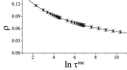
Figure 1: The density of kinks after cooling with the linear schedule. Square symbols are obtained by the Monte-Carlo simulation. The fitting curve is given by $\rho=q/\hat{\xi}$ with the correlation length $\hat{\xi}$ determined by eq. (16) with $\tau=p\tau^{\rm mc}$. Parameters $p$ and $q$ are determined by denotes of the method of least squares.

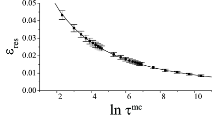
Figure 2: The residual energy obtained by Monte-Carlo simulation (square symbols). The fitting function is given by $\varepsilon_{\rm res}=\frac{\pi^{2}}{24}/(r\hat{\beta})^{2}$ with $\hat{\beta}$, the solution of eq. (18) with $\tau=p\tau^{\rm mc}$. The fitting parameter $r$ is determined by the method of least squares with $p$ given from fitting of density of kinks.

Square symbols in Fig. 1 and Fig. 2 show the density of kinks and the residual energy per spin respectively obtained by the Monte-Carlo simulation. The density of kinks is defined by $\rho=[\frac{1}{2N}\sum_{i}(1-\langle\sigma_{i}\sigma_{i+1}\rangle)]_{\rm av}$, where $\langle\cdots\rangle$ denotes the expectation value with respect to the state after simulated annealing and $[\cdots]_{\rm av}$ means the average over configurations of coupling constants.

In order to obtain fitting curves for the density of kinks and the residual energy per spin, we need to modify eqs. (17) and (19). First, we have to care about the difference in the unit of time between the Glauber’s dynamics and the Monte-Carlo dynamics. Then we bring up the relation, $\tau=p\tau^{\rm mc}$, between the inverse of quench rate $\tau$ in the Glauber’s dynamics and $\tau^{\rm mc}$ in the Monte-Carlo dynamics, where $p$ is an adjustable parameter. Next, we relate the density of kinks $\rho$ to the correlation length $\xi$ by $\rho=q/\hat{\xi}$, where $\hat{\xi}$ is the solution of eq. (16). The parameter $q$ tunes the inverse of correlation length to the density of kinks. Finally, we propose an ansatz that the residual energy is represented by $\varepsilon_{\rm res}=(\pi^{2}/24)/(r\hat{\beta})^{2}$ with an adjustable parameter $r$, where $\hat{\beta}$ is given from eq. (18) with $\tau=p\tau^{\rm mc}$.

Parameters $p$ and $q$ are determined by the method of least squares described as follows. The Monte-Carlo simulation yields a set of data $(\rho_{i},\tau^{\rm mc}_{i})$, where $\rho_{i}$ is the mean value produced by Monte-Carlo simulations. The fitting function given by eq. (17) but $\rho=q/\hat{\xi}$ and $\tau=p\tau^{\rm mc}$ does not yield $\rho$ for given $\tau^{\rm mc}$ analytically. Then we regard $\tau^{\rm mc}$ as a function of $\rho$ and define the error between Monte-Carlo data and the fitting function by $S(p,q)\equiv\sum_{i}(\ln\tau^{\rm mc}(\rho_{i})-\ln\tau^{\rm mc}_{i})^{2}/\sigma_{i}^{2}$ where $\tau^{\rm mc}(\rho_{i})$ is the value of the fitting function and $\tau^{\rm mc}_{i}$ is given from the Monte-Carlo data for $\rho_{i}$. $\sigma_{i}^{2}$ is the dispersion of $\rho_{i}$. We assume that the relative values of the dispersion between different $i$’s are the same in $\rho$ and $\ln\tau^{\rm mc}$. By minimizing $S(p,q)$, we fix the value of $p$ and $q$. The errors of $p$ and $q$ are given by $\sigma_{p}^{2}=\frac{2S}{m-2}\frac{\partial^{2}S}{\partial q^{2}}\frac{1}{D}$ and $\sigma_{q}^{2}=\frac{2S}{m-2}\frac{\partial^{2}S}{\partial p^{2}}\frac{1}{D}$, where $m$ is the number of Monte-Carlo data and $D=\frac{\partial^{2}S}{\partial p^{2}}\frac{\partial^{2}S}{\partial q^{2}}-(\frac{\partial^{2}S}{\partial p\partial q})^{2}$. The other parameter $r$ is determined by the method of least squares with the error $S^{\prime}(r)\equiv\sum_{i}(\varepsilon(\tau^{\rm mc}_{i})-\varepsilon_{i})^{2}/\sigma_{\varepsilon i}^{2}$ between the value of fitting function, eq. (19), with $\hat{\beta}_{i}$ given by eq. (18) with $\tau_{i}=p\tau^{\rm mc}_{i}$ and the value of Monte-Carlo data $\varepsilon_{i}$. $\sigma_{\varepsilon i}^{2}$ is the dispersion of $\varepsilon_{i}$. $p$ is fixed by fitting of $(\rho,\tau^{\rm mc})$. The error of $r$ is given by $\sigma_{r}^{2}=\frac{S^{\prime}}{m-1}(\frac{\partial^{2}S^{\prime}}{\partial r^{2}})^{-1}$. The obtained values of $p$, $q$ and $r$ are $q\approx 0.241\pm 0.001$, $p\approx 22.0\pm 0.9$, and $r\approx 2.14\pm 0.16$.

Figure 1 and 2 shows that results of Monte-Carlo simulation on the density of kinks and the residual energy are excellently fitted by the curves made from eq. (17) and (19) respectively. Therefore the analytic results on the basis of the Kibble-Zurek argument is confirmed by the Monte-Carlo simulation.

5 Conclusion

We studied the dynamics of quenching temperature of pure and random Ising chains, on the basis of the Kibble-Zurek argument. We showed for the pure Ising chain that the density of kinks after quenching decays as $1/\sqrt{\tau}$ for large $\tau$. As for the random Ising chain with $J_{i}\in[0,1]$, the density of kinks and the residual energy decay as $1/\ln\tau$ and $1/(\ln\tau)^{2}$ for large $\tau$ respectively. Results for the random Ising chain were confirmed by the Monte-Carlo simulation. Comparing our results on the density of kinks with known results for the quantum quench, densities of kinks after the classical quench and the quantum quench decay with the same power of $\tau$ in the pure system. As for the random Ising chain, the power of $\ln\tau$ by the quantum quench is twice as large as that by the classical quench. The difference between the quantum quench and the classical quench is substantial.

The classical quench and the quantum quench toward the ground state correspond to simulated annealing and quantum annealing respectively of an optimization problem. The random Ising chain studied in the present paper provides an optimization problem with the trivial solution. However it is a non-trivial problem for simulated annealing and quantum annealing since their dynamics toward the solution respond to randomness and exhibit the slow relaxation. Our results reveal that the random Ising chain is a solid example for which quantum annealing certainly performs better than simulated annealing.

The author thanks T. Caneva, G. E. Santoro, and H. Nishimori for fruitful discussions. The present work was partially supported by CREST, JST.

References

References

- [1] M. Greiner, O. Mandel, T. Esslinger, T. W. Hänsch, and I. Bloch, Quantum phase transition from a superfluid to a Mott insulator in a gas of ultracold atoms, 2002 Nature 415 39
- [2] L. E. Sadler, J. M. Higbie, S. R. Leslie, M. Vengalattore, and D. M. Stamper-Kurn, Spontaneous symmetry breaking in a quenched ferromagnetic spinor Bose-Einstein condensate, 2006 Nature 443 312
- [3] C. N. Weiler, T. W. Neely, D. R. Scherer, A. S. Bradley, M. J. Davis, and B. P. Anderson, Spontaneous vortices in the formation of Bose-Einstein condensates, 2008 Nature 455 948
- [4] S. Kirkpatrick, C. D. Gelett, and M. P. Vecchi, Opimization by simulated annealing, 1983 Science 220 671
- [5] A. B. Finnila, M. A. Gomez, C. Sebenik, C. Stenson, and J. D. Doll, Quantum annealing: a new method for minimizing multidimensional functions, 1994 Chem. Phys. Lett. 219 343
- [6] T. Kadowaki and H. Nishimori, Quantum annealing in the transverse Ising model, 1998 Phys. Rev. E 58 5355
- [7] E. Farhi, J. Goldstone, S. Gutmann, J. Lapan, A. Lundgren, and D. Preda, A quantum adiabatic evolution algorithm applied to random instances of an NP-complete problem, 2001 Science 292 472
- [8] A. Das and B. K. Chakrabarti, Eds., Quantum Annealing and Related Optimization Methods, Lecture Notes in Physics 2005 Springer-Verlag, Berlin
- [9] T. W. B. Kibble, Some implications of a cosmological phase transition, 1980 Phys. Rep. 67 183
- [10] W. H. Zurek, Cosmological experiments in superfluid helium?, 1985 Nature 317 505
- [11] W. H. Zurek, U. Dorner, and P. Zoller, Dynamics of a quantum phase transition, 2005 Phys. Rev. Lett. 95 105701
- [12] J. Dziarmaga, Dynamics of a quantum phase transition: exact solution of the quantum Ising model, 2005 Phys. Rev. Lett. 95 245701
- [13] J. Dziarmaga, Dynamics of a quantum phase transition in the random Ising model: logarithmic dependence of the defect density on the transition rate, 2006 Phys. Rev. B 74 064416
- [14] T. Caneva, R. Fazio, and G. E. Santoro, Adiabatic quantum dynamics of a random Ising chain across its quantum critical point, 2007 Phys. Rev. B 76 144427
- [15] P. Laguna and W. H. Zurek, Density of kinks after a quench; when symmetry breaks, how big are the pieces?, 1997 Phys. Rev. Lett. 78 2519
- [16] D. A. Huse and D. S. Fisher, Residual energies after slow cooling of disordered systems, 1986 Phys. Rev. Lett. 57 2203
- [17] R. J. Glauber, Time-dependent statistics of the Ising model, 1963 J. Math. Phys. 4 294
- [18] D. Dhar and M. Barma, Effect of disorder on relaxation in the one-dimensional Glauber model, 1980 J. Stat. Phys. 22 259
- [19] D. S. Fisher, Critical behavior of random transverse-field Ising spin chains, 1995 Phys. Rev. B 51 6411